Article

Achieving Robust Learning Outcomes in Autonomous Driving with DynamicNoise Integration in Deep Reinforcement Learning

1
College of Instrumentation and Electrical Engineering, Jilin University, Jilin 130061, China
2
School of Communication Engineering, Jilin University, Jilin 130012, China
3
School of Transportation Science and Engineering, Jilin Jianzhu University, Changchun 130118, China
4
Department of Computer Science, University of Bristol, Bristol BS8 1QU, UK
*
Author to whom correspondence should be addressed.
Drones 2024, 8(9), 470; https://doi.org/10.3390/drones8090470
Submission received: 9 August 2024 / Revised: 29 August 2024 / Accepted: 30 August 2024 / Published: 9 September 2024

Abstract

:
The advancement of autonomous driving technology is becoming increasingly vital in the modern technological landscape, where it promises notable enhancements in safety, efficiency, traffic management, and energy use. Despite these benefits, conventional deep reinforcement learning algorithms often struggle to effectively navigate complex driving environments. To tackle this challenge, we propose a novel network called DynamicNoise, which was designed to significantly boost the algorithmic performance by introducing noise into the deep Q-network (DQN) and double deep Q-network (DDQN). Drawing inspiration from the NoiseNet architecture, DynamicNoise uses stochastic perturbations to improve the exploration capabilities of these models, thus leading to more robust learning outcomes. Our experiments demonstrated a 57.25% improvement in the navigation effectiveness within a 2D experimental setting. Moreover, by integrating noise into the action selection and fully connected layers of the soft actor–critic (SAC) model in the more complex 3D CARLA simulation environment, our approach achieved an 18.9% performance gain, which substantially surpassed the traditional methods. These results confirmed that the DynamicNoise network significantly enhanced the performance of autonomous driving systems across various simulated environments, regardless of their dimensionality and complexity, by improving their exploration capabilities rather than just their efficiency.

1. Introduction

The emergence of autonomous driving technology marks a pivotal shift in the transportation sector, with profound implications for road safety [1], efficiency [2], and accessibility [3]. By utilizing advanced sensors, machine learning, and artificial intelligence, autonomous vehicles have been designed to minimize human error—the primary cause of road accidents. This reduction is expected to substantially decrease the incidence of collisions, injuries, and fatalities. Beyond enhancing safety, autonomous driving technology promises to transform access for populations with limited mobility, such as the elderly and disabled, thus providing increased independence. Additionally, these vehicles are engineered to optimize routing and traffic management [4], which could [5] alleviate congestion and lower environmental impacts through the promotion of more efficient fuel usage and accelerating the adoption of electric vehicles. The potential applications of autonomous driving are extensive, where they encompass personal and public transport, logistics, and delivery services, and thus, transform urban environments and fundamentally alter our interaction with travel.
To advance the development of vehicles that can navigate and operate autonomously without human intervention, traditional control methodologies, such as [6,7] proportional–integral–derivative (PID) controllers and model predictive control (MPC) [8], provide distinct approaches to automation. PID controllers are lauded for their simplicity, which minimizes the discrepancy between the desired trajectory and the actual position of the vehicle. This method is easy to implement and performs effectively under stable conditions, which makes it ideal for straightforward applications, such as cruise control. However, its reactive nature is less effective in dynamic, complex environments, where the ability to anticipate future conditions is crucial. In contrast, MPC is distinguished by its capacity to incorporate future states and constraints, thus optimizing control inputs across a predictive horizon. This forward-thinking approach enables MPC to proficiently manage intricate driving situations, such as obstacle avoidance and adaptive cruise control. Despite its benefits, the computational intensity of MPC presents challenges for real-time implementation, underscoring a significant trade-off between predictive accuracy and computational efficiency.
In traditional reinforcement learning tasks [9], the deep Q-network (DQN) has gained widespread application [10] due to its benefits in end-to-end learning, stability, and efficiency, which make it valuable for addressing problems in environments with discrete action spaces [11]. However, DQN only applies to discrete action spaces; other schemes are needed for continuous action spaces. The soft actor–critic (SAC) algorithm [12] is characterized by its high sampling efficiency, and better stability and convergence can be achieved through both value and policy functions. In addition, SAC is particularly effective for tasks with a continuous action space, which makes it suitable for applications such as autonomous driving. However, these methods face common challenges, including slow convergence rates, insufficient exploration, issues with time delays, and sub-optimal reward outcomes.
To address these issues, we propose a network framework named DynamicNoise, which introduces an innovative approach to enhance the network performance. One of the critical challenges in reinforcement learning is effectively balancing exploration and exploitation. Traditional methods, such as the ε -greedy algorithm, often fall short in facilitating sufficient exploration, which lead to sub-optimal policies. Our DynamicNoise network employs a straightforward strategy to balance exploration and exploitation [13] through the incorporation of noise into the network architecture. This modification, which is achieved with a singular adjustment of the weight vector, induces a consistent yet complex alteration in the policy, which is dependent on the state over multiple time steps and contrasts sharply with jittering strategies that insert uncorrelated noise, such as the ε -greedy strategy, at each decision point.
The main contributions of our work are as follows:
1. Enhanced exploration in 2D environments: We employed Markov models for environmental inputs (e.g., vehicle speed, location, and destination) and action decisions (including acceleration and turning) in the DQN and DDQN, respectively, in a 2D setting. Subsequently, we introduced random-valued noise to optimize the vehicle-turning process, thus significantly improving the exploration and policy robustness.
2. Application in realistic 3D scenarios: To validate the applicability of our framework in more realistic scenarios, as well as with different network architectures, we introduced noise into the action selection and fully connected layers of the SAC model in a 3D environment to optimize the process of actual vehicle driving. This approach enhanced the exploration capabilities of the SAC model and led to a better performance in complex driving environments.
3. Comprehensive validation and future implications: We first validated the feasibility of the algorithm in a two-dimensional scenario and then demonstrated the superiority of the algorithm in a more realistic three-dimensional scenario. The results indicate that our DynamicNoise framework could more effectively accomplish the autonomous driving navigation task. The application of the DynamicNoise framework could be extended to similar operating environments, which suggests broad implications for future research and applications of autonomous systems.
The remainder of this paper is organized as follows: Section 2 reviews the related literature. Section 3 describes the methodology. Section 4 presents the experimental setup. Section 5 discusses the results. Finally, Section 6 concludes the paper and suggests future research directions.

2. Related Work

While autonomous driving has many challenges regarding its complexity and dynamics, riding on the development of machine learning techniques, reinforcement learning has led to breakthroughs in the field.
Alizadeh et al. [14] established a decision-making and planning model based on the DQN algorithm that showed better performance than the traditional method in a noisy environment with different noise levels. Unfortunately, DQNs are not without their challenges: One major drawback of such an approach is the slow convergence rate, which may not allow for real-time adaptation in dynamic driving scenes. Furthermore, poor exploration may result from poor policy learning when using a DQN.
Some of the limitations of DQNs were addressed by creating the DDQN algorithm. Double Q-learning, which was proposed by Hasselt et al. [15], mitigates the overestimation bias in Q-learning and acts as the genesis point for the development of the DDQN, which has been commonly used in the context of autonomous driving. Liao et al. [16] used the DDQN to address high-level decision-making problems with large state spaces and obtained good safety results and performance. The DDQN can still lead to high-decision-time delays under binary action spaces, thus offering sub-optimal reward outcomes.
Seong et al. [17] employed the SAC method to propose a spatio-temporal attention mechanism to assist in the decision-making method for managing autonomous driving at intersections. SAC algorithms, which are highly sample efficient and stable, perform well in complex driving scenarios. Nevertheless, similar to the DQN and DDQN, SAC also needs to improve its convergence and exploration problems, which can become ineffective, especially when considering a quickly changing environment.
Lillicrap et al. [18] proposed continuous control with deep reinforcement learning, which has been instrumental in developing algorithms such as DDPG for more granular control in autonomous driving tasks. Schulman et al. [19] developed proximal policy optimization (PPO), which is another popular RL algorithm used for continuous control tasks in autonomous driving.
Chen et al. [20] developed a safe reinforcement learning approach that integrates human driver behavior by utilizing regret theory to determine whether to change lanes or maintain the current lane. This composite model allows agents to learn safe and stable driving strategies that mimic human decision-making processes. Although this method still needs to improve its inefficiencies, it laid the groundwork for improved approaches by enhancing the safety and stability of autonomous driving strategies by incorporating human decision-making models.
Building on this, He et al. [21] adopted a constrained-observation robust Markov decision process to simulate lane-changing behavior in autonomous vehicles. Employing Bayesian optimization for black-box attacks, they effectively approximated optimal adversarial observation perturbations. Their algorithm demonstrated excellent generality and robustness in the face of observational perturbations, thus further enhancing the stability of autonomous driving systems in complex and uncertain environments. However, they did not verify continuous action spaces, and thus, could not address longitudinal decision-making problems in autonomous vehicles.
To further mitigate driving risks, Li et al. [22] proposed a new method based on risk assessment using a probabilistic model to evaluate the risk and apply it to reinforcement learning driving strategies. This approach aimed to minimize driving risks during lane-changing maneuvers, which ensures safer decision-making processes. This research built on previous work by focusing on risk management and safety enhancement. However, such methods still need to consider integrating different decision-making layers with various approaches to increase the complexity of decision-making tasks.
Peng et al. [23] decoupled speed- and lane-changing decisions, thus training them separately using different reinforcement learning methods to address the complexity of decision making in driving tasks. This separation helped to overcome the training difficulties caused by the coupling of these tasks, thus leading to more efficient learning and strategy optimization. However, this method does not allow for the simultaneous inclusion of lane-change trajectories during the research process. Additionally, the model performed poorly in situations characterized by high speeds and small distances between vehicles.
Hoel et al. [24] combined Bayesian reinforcement learning with a random prior function (RPF) to estimate the confidence of actions, which yielded more reliable action outputs at intersections under high uncertainty and reduced the likelihood of collisions. This study enhanced the reliability of decision making under uncertain environments through confidence evaluation. However, how to systematically set the parameter values was not specified, nor could these parameter values be automatically updated during the training process.
Finally, Zhang et al. [25] incorporated traffic rules into a reinforcement learning algorithm by integrating the priority of surrounding vehicles into the state space. Combining this with responsibility-sensitive safety (RSS) detection, they were able to control the longitudinal speed more effectively, thus assisting vehicles in ensuring their safe driving in various traffic scenarios. This study further enhanced the practicality and safety of autonomous driving systems by combining rules and safety detection.
Despite these successes, balancing exploration and exploitation remains a challenge [26]. Studies explored value penalty factors and policy normalization to align the learned policies with expert behaviors. Lillicrap et al. [27] explored techniques for training exploration strategies using correlated noise, but these techniques may face difficulties under more variable conditions. Plappert et al. [28] introduced a technique that involved constant Gaussian noise in the network. Unlike these works, the method proposed in this study allows for the dynamic adjustment of noise applications over time that are not limited to the Gaussian mode, thereby enhancing its adaptability and effectiveness in different driving environments.
Adding noise introduces new exploration opportunities, and while it can effectively handle uncertainties within the training environment, it may struggle to address novel, unseen uncertainties in real-world scenarios. To overcome this issue, Hunmin et al. [29] proposed an active, robust adaptive control architecture for autonomous vehicles across various environments. This architecture estimates unknown cornering stiffness using weather forecasts and vehicle network data to effectively balancing performance and robustness. Currently, systems increasingly rely on machine learning. Although many scholars proposed effective techniques to demonstrate the robustness of predictions against adversarial input perturbations, these techniques often diverged from the downstream control systems that used these predictions. Jinghan et al. [30] addressed this by providing robust certification of control against adversarial input perturbations through robust control of the original input disturbances. This enhances the certification security to ensure reliable operation under a broader range of unpredictable conditions.

3. Methods

3.1. Markov Decision Process Modeling

The usefulness of the MDP has led to its continuous use in reinforcement learning. The MDP is characterized by the tuple (S, R, A, γ , T), where S denotes the state space; R denotes the reward function; A denotes the action space; γ denotes the discount factor; and T denotes the transition model, which describes the probability of transitioning from one state to another.

3.1.1. State Space

State Space in DQN Variants

The most critical aspect of successful autonomous driving is determining the state of the vehicle itself and its surrounding environment. Relying on a single state makes it difficult for each vehicle to make optimal decisions. Therefore, we introduce a multi-dimensional state. In our model, the state configuration included the observation information of the autonomous vehicles. Specifically, the observation type was “Kinematics”, and the number of observed vehicles was 15. We selected a series of features to describe the state of each vehicle, including the presence of the vehicle, x-coordinate (measured in meters, m), y-coordinate (measured in meters, m), velocity in the x-direction (measured in meters per second, m/s, v x ), velocity in the y-direction (measured in meters per second, m/s, v y ), and the cosine ( c o s h ) and sine ( s i n h ) of the heading angle.
The value ranges for these features were as follows: the x-coordinate ranged from −100 to 100 m, the y-coordinate ranged from −100 to 100 m, the velocity in the x-direction ranged from −20 to 20 m per second, and the velocity in the y-direction ranged from −20 to 20 m per second.
Additionally, we used absolute coordinates to describe these features without flattening the observation matrix or considering the intentions of other vehicles. The number of controlled vehicles was set to 1, the initial vehicle count was 10, and the probability of spawning a new vehicle was 0.6. This multi-dimensional state representation helped the model to make more accurate and effective decisions in various traffic scenarios.

State Space in SAC

An RGB image was created by stitching together outputs from three 60-degree cameras mounted on the car roof, which resulted in a 180° wide-angle view. This stitched RGB image had a size of 3 × 84 × 252. For training purposes, three consecutive images were stacked to capture temporal information, which made the final input to the model a tensor with a shape of 9 × 84 × 252. This configuration allowed the model to utilize both spatial and temporal features for more robust learning.

3.1.2. Action Space

Actions in DQN Variants

In our model, the action configuration defines the operations that autonomous vehicles can undertake. We set the action type to DiscreteMetaAction, which meant the vehicles could select from predefined discrete actions. The action space included the following three operations:
  • Decelerate (target velocity: 0 units);
  • Maintain speed (target velocity: 4.5 units);
  • Accelerate (target velocity: 9 units).
These actions primarily control the vehicle’s longitudinal movement, which allow it to adjust its speed in response to different driving scenarios. While the action space does not explicitly include lateral actions, such as turning, the vehicle’s ability to navigate intersections and perform turns is achieved through the manipulation of its velocity components ( v x and v y ) and heading direction (represented by c o s h and s i n h ). This approach enables the vehicle to change direction smoothly by adjusting the direction of its velocity vector within the physical simulation of the environment.
To clarify, the turning mechanism in our model is implicitly managed by the vehicle’s kinematic model. Although the action space is limited to longitudinal controls, the vehicle can still navigate intersections by adjusting the direction of its velocity vector through the simultaneous adjustment of the v x and v y components. The heading direction, as represented by c o s h and s i n h , also plays a crucial role in this process by allowing the vehicle to follow the appropriate trajectory and make smooth turns without the need for explicit lateral actions.
By focusing on these essential longitudinal actions with specific target velocities, the model ensures operational stability and responsiveness while maintaining the flexibility to perform complex maneuvers, such as turning at intersections, through the underlying kinematic adjustments. This design reduces any unnecessary complexity and allows the model to effectively control the movement of the vehicle in diverse and dynamic driving environments.

Actions in SAC

The action space is composed of two amplitude control dimensions: steering amplitude control and brake (acceleration) amplitude control. The steering amplitude control was normalized to the continuous interval [0, 1], and in practice, it operated within a continuous range of continuous_steer_range [−0.3, 0.3] radians (approximately −17.19 to 17.19 degrees). This allowed the vehicle to adjust its direction within this range. The brake amplitude control, which was also normalized to the [0, 1] interval, corresponded to the vehicle’s acceleration control, which was defined by the continuous_accel_range of [−3.0, 3.0] m/s². Positive values of this control result in acceleration, while negative values manage braking or deceleration.

3.1.3. Reward Function

Reward in DQN Variants

In our task, vehicles traveling at high speeds, staying in their designated lanes, avoiding collisions, and successfully reaching the destination were rewarded. The reward function is defined according to Formula (1):
R = ( W c o l l i s i o n × R c o l l i s i o n + W s p e e d × R s p e e d + W a r r i v e d × R a r r i v e d ) × R l a n e ,
where R is the total reward, R c o l l i s i o n is the collision reward, R s p e e d is the speed reward, and  R l a n e is the lane reward. R c o l l i s i o n , R s p e e d , and  R l a n e are computed according to Formulas (2), (3), and (4), respectively:
R c o l l i s i o n = 5 , if the car crashed , 0 , otherwise ,
R speed = 1 , if Speed > 9 , Speed 7 2 , if 7 < Speed 9 , 0 , otherwise .
R l a n e = 1 , if the car is on road , 0 , if the car is not on road .
If arrived_reward is True, then we use Formulas (5) and (6):
R = R a r r i v e d ,
R a r r i v e d = 1 , if the car arrives , 0 , if the car does not arrive .
In the above formulas, W c o l l i s i o n , W s p e e d , and  W l a n e are hyperparameters used to determine the importance of speed, lane adherence, and safety. Each vehicle was represented as a rectangle (5 m long and 2 m wide) in this environment. A collision occurs if there is an overlap between the rectangle corresponding to the autonomous vehicle and those corresponding to other vehicles.

Reward in SAC

The reward is described by Formula (7):
r t ( s , a ) = v T u ^ Δ t C i I C s steer ,
where v T u ^ represents the actual speed of the vehicle projected onto the road’s effective speed. This term encourages the vehicle to maintain an optimal speed along the direction of the road to maximize the effective distance travelled during the time step Δ t .
I is the impact force (N/s) obtained through sensors, which represents the external forces acting on the vehicle. A higher impact force results in a greater penalty, thus discouraging aggressive or unsafe driving behaviors. The coefficient C i determines the severity of this penalty.
steer is the magnitude of the steering control, which reflects the extent of the steering input. Excessive steering, which could lead to instability, is penalized more heavily. The penalty is scaled by the coefficient C s , which adjusts the impact of steering control on the overall reward.
This reward function is designed to balance the trade-offs between maintaining an efficient speed, minimizing impact forces, and avoiding erratic steering, thereby promoting stable and safe driving behaviors.

3.1.4. Discount Factor: γ

In the context of autonomous vehicles, particularly when considering models focused on turning and obstacle avoidance, the discount factor ( γ ) is instrumental in shaping the learning process. This factor is crucial for balancing immediate and long-term goals, thereby enhancing the efficiency and stability of learning outcomes. An appropriately calibrated discount factor not only prompts the vehicle to execute safe and effective maneuvers in critical situations but also enhances the overall efficiency and comfort of the journey. Doing so ensures that the developed driving strategies are optimal regarding safety and practical usability. Therefore, carefully selecting the discount factor is vital for achieving efficient and secure autonomous driving operations.
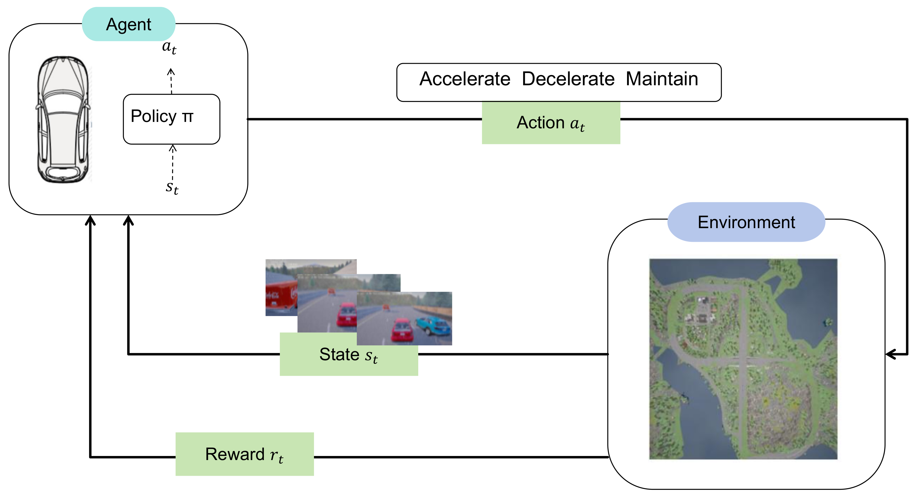
In the MDP, the action space A t and reward function R t are incorporated into the foundational structure of a Markov process. We can conceptualize A t as the input of the system and R t as its output. In this framework, as shown in Figure 1, the state transitions within the MDP are influenced externally rather than solely by internal processes; that is, they are determined by the current state S t and the input A t . Consequently, the subsequent state S t + 1 is dictated by the transition probability model P ( S t + 1 | S t ) and, similarly, R t is defined by the probability distribution P ( R t | S t , A t ) , which, for simplicity, can be denoted as R t ( S t , A t ) .
In the realm of RL, the environment responds by assigning a reward according to the action of the agent and the current state. The RL model aims to discover the optimal policy by maximizing this reward. For example, the policy for navigating intersections, as shown in Figure 2, represents a specific type of MDP, where the autonomous vehicle (AV) acts as an intelligent agent. This agent enhances the performance through dynamic interactions with other vehicles, and thus, continuously learns and adapts. The delineation of a policy within the context of this MDP involves precise definitions of these interactions and the resultant learning mechanisms.

3.2. The Proposed Framework

3.2.1. Overview
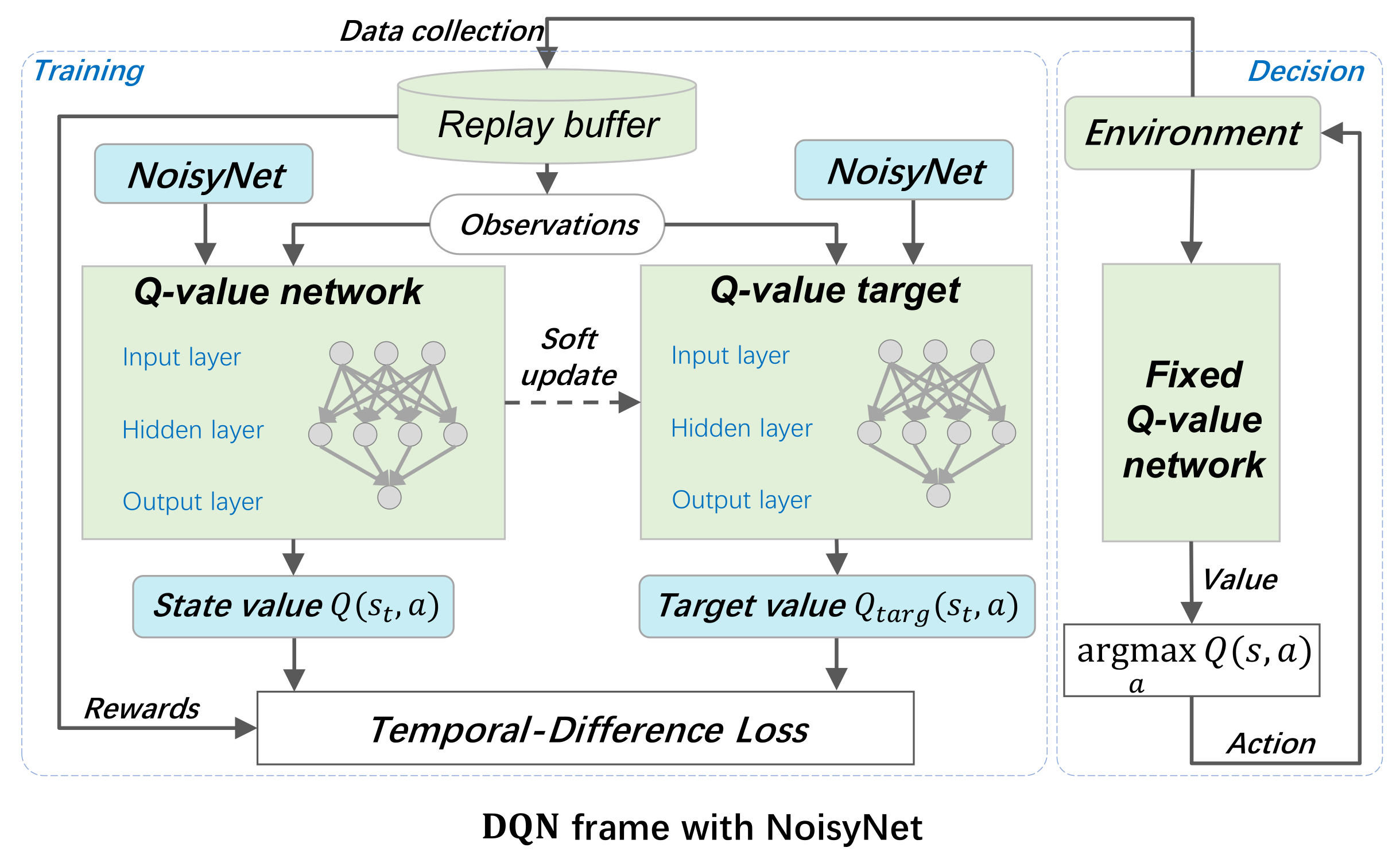
The DynamicNoise framework represents a comprehensive approach to enhancing deep reinforcement learning capabilities to cope with complex dynamic environments. At the core of the framework is the integration of high-level variants of the standard DQN models and SAC models to better address the challenges faced by autonomous systems, with a particular focus on increasing exploration and improving the accuracy of decision making.
The proposed DynamicNoise framework consists of two modules: NoisyNet based on the DQN model and NoisyNet based on the SAC model, where NoisyNet based on the DQN model consists of the DQN and the DDQN. Each of these components is designed to take advantage of the intrinsic strengths of the basic model while introducing a noise mechanism that enhances the exploration through the injection of noise.
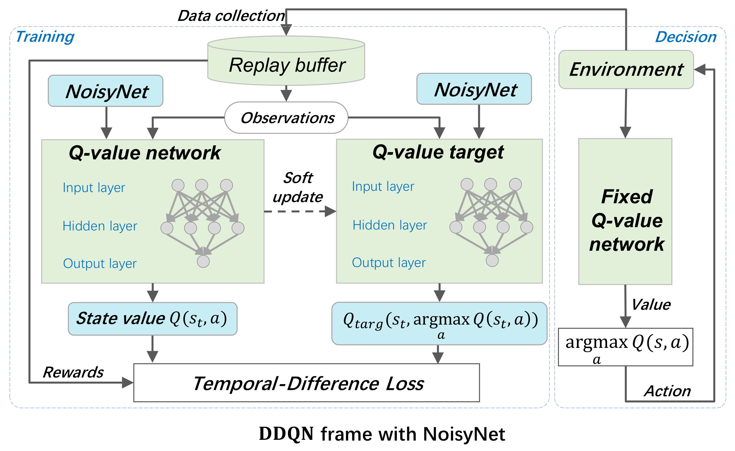
1. DQN model: This component modifies the traditional DQN by adding NoisyNet and introducing parameter noise into the network weights. The flowchart of the network is represented in Figure 3. This noise enriches the policy exploration, which allows the network to explore a more diverse set of actions without explicitly exploring specific hyperparameters, which is similar to ε in the ε -greedy policy. Building on the DQN using NoisyNet, the DDQN using NoisyNet is made more efficient and effective by using two separate networks to extend the framework, as in the traditional DDQN approach. This setup helps to reduce the overestimation of the action values, which often occurs in the standard DQN models. The flowchart of this network is simply represented in Figure 4. Adding NoisyNet to the policy and target networks can further facilitate exploration and help speed up the convergence by providing a wider range of experience during training.
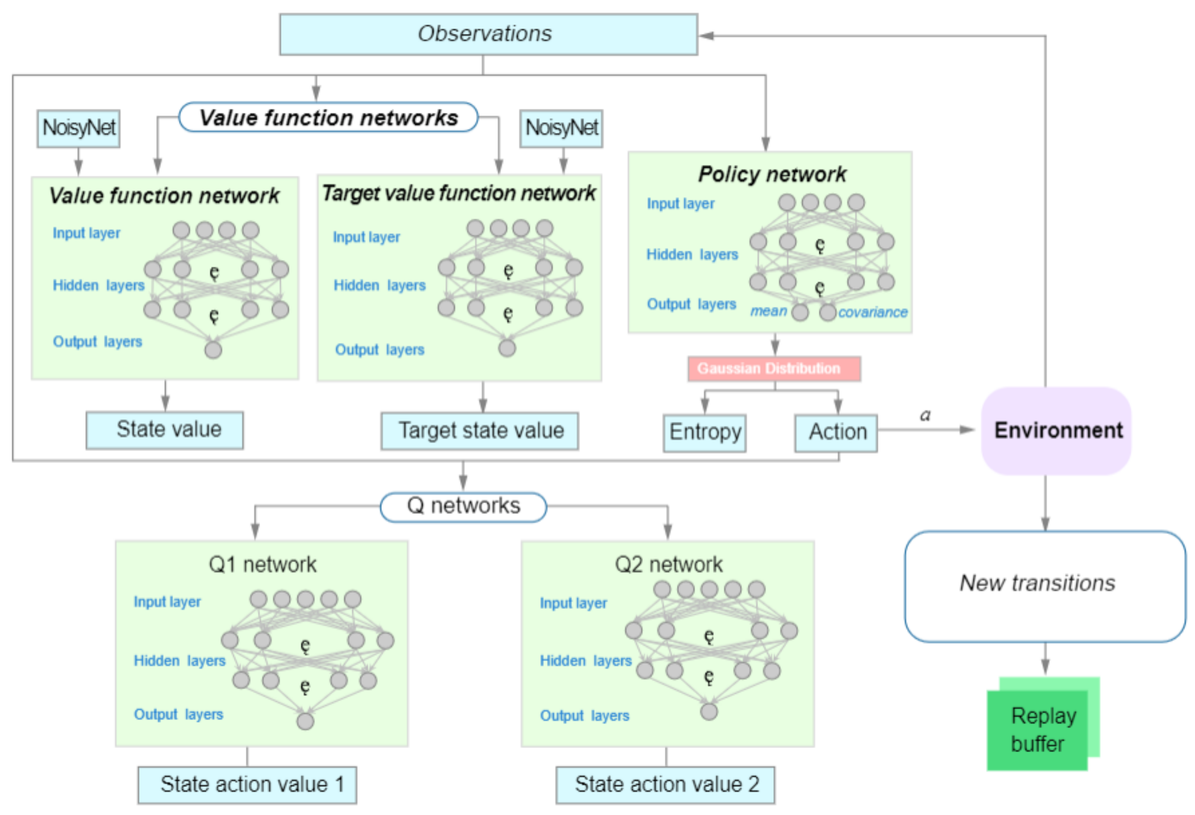
2. SAC model: This component modifies the traditional SAC by adding NoisyNet and introducing parameter noise into the network weights. The network flow is represented in Figure 5. This noise enriches the exploration of strategies, thus making the NoisyNet SAC framework more efficient and effective. This setup helps to reduce the bias in the value estimation that often occurs when using standard SAC models.
Figure 3. Flowchart of DQN with NoisyNet.
Drones 08 00470 g003
Figure 4. Flowchart of DDQN with NoisyNet.
Drones 08 00470 g004
Figure 5. Flowchart of SAC with NoisyNet.
Drones 08 00470 g005

3.2.2. DQN with NoisyNet

Through practical research, we found that the exploitation capability of the DQN alone was insufficient. Therefore, we modified the DQN to enhance its exploitation abilities.
We changed the traditional exploration mechanism by enhancing the DQN by introducing parametric noise into its network weights. Specifically, in the neural network of the DQN, each weight is no longer a fixed value but a random variable determined by a fixed mean parameter and a learnable variance parameter. In this way, each forward propagation of the network produces a different result that depends on the randomness of the weights, thus introducing exploration ability into the decision-making process of agents. Unlike traditional ε -greedy exploration or noise-adding strategies, NoisyNet allows the exploration behavior of the agent to adapt, along with the learning process, which is achieved by optimizing the variance parameters of the weighted noise.
When the noise layer replaces the linear layer, the parametric action value function Q ( x , a , ε ; ζ ) can be considered a random variable. In particular, a dense neural network layer that inputs p dimensions and outputs q dimensions is expressed as y = ω · x + b . The respective noisy layer is characterized by Formula (8):
y = ( μ ω + ϵ ω σ ω ) x + ( μ b + ϵ b σ b ) ,
where μ ω , σ ω R p × q and σ b , μ b R q are trainable parameters, and  ϵ ω R p × q and ϵ b R q are noises. Given that the loss of a noisy network is represented as an expectation over noise, the gradient can be calculated using L ( ζ ) = E [ L ( θ ) ] . In noisy networks, the parameters of the original DQN can be replaced with trainable parameters, as shown in Formula (9):
L ¯ ( ζ ) = E [ E ( x , a , r , y ) D [ r + γ max b a Q ( y , b , ϵ ; ζ ) Q ( y , a , ϵ ; ζ ) ] 2 ] .
The DQN stands out as a typical algorithm in the field of value-based reinforcement learning [31]. It leverages the temporal difference (TD) error as the loss function for the neural network by incorporating techniques such as convolution, an experienced buffer, and random experience replay. The DQN has achieved human-level performance in the domain of Atari games. At each time step, as shown in Algorithm 1, the environment offers the agent an observation s t . Initially, the agent selects an action following the ε -greedy strategy and receives a response r t and the subsequent state s t + 1 from the environment. Subsequently, the tuple ( s t , a t , r t , s t + 1 ) is added to the experience buffer, and we obtain Formula (10):
L ( θ ) = E [ ( r t + γ max a Q π ( s t + 1 , a ; θ ) Q π ( s t , a t ; θ ) ) 2 ] ,
where θ represents the parameters of the online network, while θ denotes the parameters of the target network. The parameters θ are periodically updated to match θ at regular intervals.

3.2.3. DDQN with NoisyNet

Building upon the DynamicNoiseDQN framework, we further explored incorporating a noise layer into the DDQN structure to enhance the exploration capabilities of the network in complex autonomous driving scenarios, particularly for tasks that involve turning and avoiding other vehicles.
The DDQN improves upon the traditional DQN method by addressing the issue of overestimated value estimations. This is achieved through two separate networks: one for action selection and the other for evaluating the value of that action. Thus, we obtain Formula (11):
Q t a r g e t = r + γ Q ( s , argmax a Q ( s , a ; θ ) ; θ ) ,
where r represents the reward, γ is the discount factor, s is the next state, θ denotes the current network parameters, and  θ denotes the target network parameters.
Algorithm 1 DQN with NoisyNet
Input: Env: Environment, ε : a set of random variables for the network, B: initialized as an empty replay buffer, ξ : initial parameters of the network, ζ : initial parameters of the target network, N B : capacity of the replay buffer, N T : batch size for training, and N : interval for updating the target network
Output: Q ( · , ε ; ξ )
1:
for episode e 1 , , M   do
2:
     Initialize state sequence x 0 E n v
3:
     for  t 1 ,  do
4:
         Set x x 0
5:
         Draw a noisy network sample ξ ε
6:
         Choose an action a a r g m a x b a Q ( x , b , ξ ; ζ )
7:
         Draw the next state y P ( · | x , a ) , obtain reward r R ( x , a ) , and set x 0 y
8:
         Receive reward B[−1] ( x , a , r , y )
9:
         if  B > N B  then
10:
            Remove the oldest transition from B
11:
         end if
12:
         Sample a minibatch of NT transitions ( ( x j , a j , r j , y j ) D ) j = 1 N T
13:
         Draw the noisy variable for the online network: ξ ε
14:
         Generate the noisy variables for the target network: ζ 0 ε
15:
         for  j 1 , , N T  do
16:
            if  y j represents an ultimate state then
17:
                 Q ^ y j
18:
            else
19:
                 Q ^ r j + γ arg max b A Q y j , b , ξ ; ζ
20:
                Perform a gradient update using the loss ( Q ^ Q ( x j , a j , ξ ; ζ ) ) 2
21:
            end if
22:
            if  t 0 ( m o d N )  then
23:
                Generate the noisy variables for the target network: ζ ξ
24:
            end if
25:
         end for
26:
     end for
27:
end for
To further enhance exploration using the DDQN, we introduced noise into the fully connected layers. The parameters of these layers are defined by the following Formula (12), where the noise component provides random perturbations to the parameters during training, thus facilitating the exploration of different strategies:
w = σ w ϵ w + μ w , b = σ b ϵ b + μ b ,
where μ w and σ w are the mean and standard deviation of the weights, respectively, and  ϵ w is the noise sampled from a probability distribution. A similar setup is applied to the bias b.
During training, the noise vector ϵ is resampled at each training step to ensure that each forward pass of the network slightly differs. This dynamic change in network parameters, as shown in Algorithm 2, not only enhances the environmental exploration but also improves the network’s adaptability to changing conditions. This is particularly valuable considering the variable conditions encountered in autonomous driving.
Through these improvements, the noise-enhanced DDQN model demonstrates superior performance in handling complex autonomous driving tasks, and effectively learns and adapts to different driving situations better than the traditional DDQN.
Algorithm 2 DDQN with NoisyNet
Input: Env: Environment, ε : a set of random variables for the network, B: initialized as an empty replay buffer, ξ : initial parameters of the network, ζ : initial parameters of the target network, N B : capacity of the replay buffer, N T : batch size for training, and N : interval for updating the target network
Output: Q ( · , ε ; ξ )
1:
for episode e 1 , , M  do
2:
     Initialize state sequence x 0 E n v
3:
     for  t 1 ,  do
4:
         Set x x 0
5:
         Draw a noisy network sample ξ ε
6:
         Choose an action a a r g m a x b a Q ( x , b , ξ ; ζ )
7:
         Draw the next state y P ( · | x , a ) , obtain reward r R ( x , a ) , and set x 0 y
8:
         Receive reward B[−1] ( x , a , r , y )
9:
         if  B > N B  then
10:
            Remove the oldest transition from B
11:
         end if
12:
         Sample a minibatch of NT transitions ( ( x j , a j , r j , y j ) D ) j = 1 N T
13:
         Draw the noisy variable for the online network: ξ ε
14:
         Generate the noisy variables for the target network: ζ 0 ε
15:
         for  j 1 , , N T  do
16:
            if  y j represents an ultimate state then
17:
                 Q ^ y j
18:
            else
19:
                 Q o n l i n e a r g m a x b A Q ( y j , b ; ξ )
20:
                 Q ^ r j + γ Q ( y j , Q o n l i n e ; ζ )
21:
            end if
22:
            Perform a gradient update using the loss ( Q ^ Q ( x j , a j , ξ ; ζ ) ) 2
23:
         end for
24:
         if  t 0 ( m o d N )  then
25:
            Update the parameters of the target network: ζ ξ
26:
         end if
27:
     end for
28:
end for

3.3. Soft Actor–Critic with Noisy Critic

To further validate the performance of our Noisynet in real-world autonomous driving scenarios, we compared SAC + Noisynet with the existing SAC framework. SAC is a reinforcement learning framework commonly used in high-dimensional continuous control scenarios with high efficiency and stability. The SAC framework consists of two main components: the critic and actor networks. The critic network is responsible for learning Q-valued functions, while the actor network is responsible for learning strategies. Critic networks evaluate the quality of the current policy by minimizing the error of the Q-value function, while actor networks update the policy by maximizing the expected reward.
The purpose of the SAC algorithm is to maximize the future cumulative reward value and entropy such that the strategy is as random as possible; that is, the probability of the output of each action is as scattered as possible rather than concentrated on one action. The objective function of the SAC algorithm can be expressed as Formula (13):
J ( π ) = t = 0 T E s t , a t ρ π r s t , a t + α H π · s t ,
where T represents the total number of time steps of the interaction between the agent and the environment; p π represents the distribution under the strategy π ( s t , a t ) ; H ( · ) represents the entropy; and  α is a hyperparameter, the purpose of which is to control the randomness of the optimal strategy and weigh the importance of entropy relative to the reward.
In our experiments, we integrated Noisynet into the SAC framework, as shown in Algorithm 3, to evaluate its performance in autonomous driving tasks. Noisynet enhances the exploration by adding noise into neural networks to help find better strategies in complex environments. Our extensive experiments on multiple simulation environments and real-world driving data revealed that SAC + Noisynet outperformed the standard SAC framework in several performance metrics.
Algorithm 3 Soft Actor–Critic with Noisy Critic
Input: Initial policy parameters θ ; Q-function parameters ϕ 1 , ϕ 2 ; and empty replay buffer D
1:
Set target parameters equal to main parameters ϕ targ , i ϕ i and ϕ targ , 2 ϕ 2
2:
repeat
3:
     Observe state s and select action a π θ ( · | s )
4:
     Execute a in the environment
5:
     Observe next state s , reward r, and done signal d to indicate whether s is terminal
6:
     Store ( s , a , r , s , d ) in replay buffer D
7:
     if  s is terminal then
8:
         Reset environment state
9:
     end if
10:
     if it is time to update then
11:
         for j in range(however many updates) do
12:
            Randomly sample a batch of transitions, B = { ( s , a , r , s , d ) } from D
13:
            Compute targets for the Q functions:
y ( r , s , d ) = r + γ ( 1 d ) min i = 1 , 2 Q ϕ targ , i ( s , a ) α log π θ ( a | s ) , a π θ ( · | s )
14:
            Update Q-functions by one step of gradient descent using
ϕ i 1 | B | ( s , a , r , s , d ) B Q ϕ i ( s , a ) y ( r , s , d ) 2 for i = 1 , 2
where  Q ϕ i ( s , a )  includes noisy layers: 
Q ϕ i ( s , a ) = Q noisy_fc ( s , a )
15:
            Define Q noisy_fc :
Q noisy_fc ( x ) = ( W + σ W ϵ W ) x + ( b + σ b ϵ b )
with ϵ W , ϵ b N ( 0 , 1 ) .
16:
            Update policy by one step of gradient ascent using
θ 1 | B | s B min i = 1 , 2 Q ϕ i ( s , a ˜ θ ( s ) ) α log π θ ( a ˜ θ ( s ) | s ) ,
where a ˜ θ ( s ) is a sample from π θ ( · | s ) , which is differentiable with respect to θ via the reparameterization trick.
17:
            Update target networks with
ϕ targ , i ρ ϕ targ , i + ( 1 ρ ) ϕ i for i = 1 , 2
18:
         end for
19:
     end if
20:
until convergence

4. Experiment

4.1. Experiment in Highway_Env

To evaluate the objectives outlined in the Introduction, we implemented the noise-enhanced DynamicNoiseDQN within a car-turning scenario at an intersection by utilizing the open-source highway_env [32] simulation platform. Specifically, the intersection-v0 environment was employed to simulate intersection dynamics, where the vehicle trajectories were created using the kinematic bicycle model. This setting enabled the vehicles to execute continuous-valued steering and throttle control actions, thereby closely replicating real-life driving scenarios.
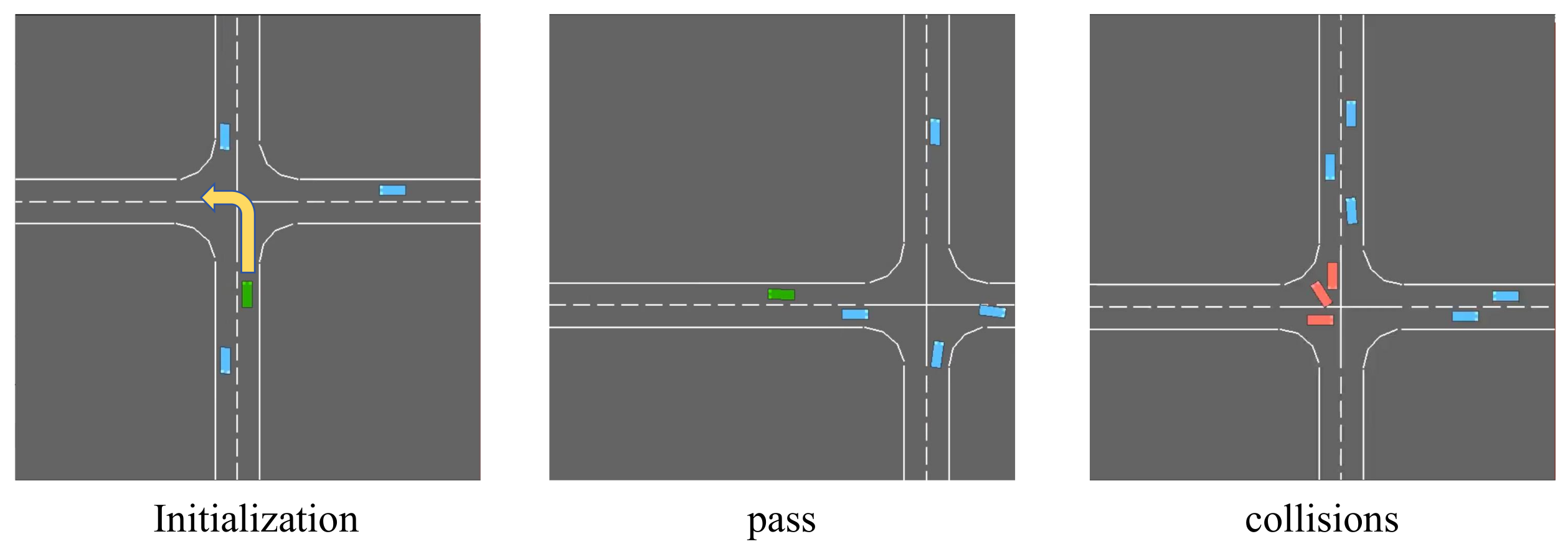
In the intersection scenario shown in Figure 6, the agent being tested (represented by a green vehicle) was tasked with executing a collision-free, unprotected left turn at a two-lane intersection in the presence of another vehicle (represented by a blue vehicle). A collision in this context is considered a rare event, with the adversarial policy reflecting the behavior of the surrounding vehicle. The primary goal was to evaluate stationary deterministic strategies, which included maintaining a constant speed and adhering to lane protocols. This involved following standard rules at intersections without traffic signals, such as yielding to vehicles approaching from the right, maintaining a safe distance, avoiding arbitrary acceleration or deceleration, and not changing lanes unpredictably. To compare the performance of the noise-enhanced network with that of a conventional DQN, ten independent and distinct experiments were conducted for each model.
To showcase the effectiveness of our proposed approach, we compared our method with contemporary, state-of-the-art traditional RL strategies, and the performance was assessed across multiple dimensions using a variety of metrics.
(a) Speed of convergence: We compared the efficiency of our model by examining the number of episodes required to reach convergence for two data sets. This was performed by calculating the average number of episodes over ten experiments and assessing whether our model demonstrated a significant improvement in efficiency.
(b) Success rate: In an autonomous driving system, safety is the primary performance indicator. In our framework, the success rate and average passing time served as general metrics for the performance assessment. The success rate directly reflected how the RL agent handles the specified task. Our framework defined the success rate according to Formula (14):
success rate = Success Counts Total Numbers × 100 % ,
(c) Time for the completion of tasks: In our analysis of successfully completed journeys, we meticulously documented the time each vehicle took to traverse from the starting point to the designated destination. The efficacy of our network strategy was directly correlated with the efficiency exhibited by the vehicles, as reflected in the average time required to accomplish the task.
For the training of the DQN, we adopted a discount factor of 0.95 and set the batch size to 64. To avoid overfitting, we limited the number of training episodes to 2000. We chose a target update value of 256 to train the noise network, with the batch size remaining at 64 and the discount factor set to 0.9. Our DynamicNoiseDQN structure was a 128 × 128 fully connected network, and the target memory_capacity value was set to 15,000. When training the DQN with the ε -greedy strategy, we set the value of ε to 0.5. In the training task for NoisyNet with the DDQN, we kept the other settings unchanged and set the value of double to 1.
In our implementation of NoisyNet, the noise was generated by sampling from a standard normal distribution and applying a non-linear transformation. Specifically, the noise ϵ was calculated using ϵ = sign ( x ) · | x | , where x N ( 0 , 1 ) . This approach ensured that the noise retained the properties of the normal distribution while providing more stable variance, thereby enhancing the model’s exploration capabilities during training.

4.2. Experiment in CARLA

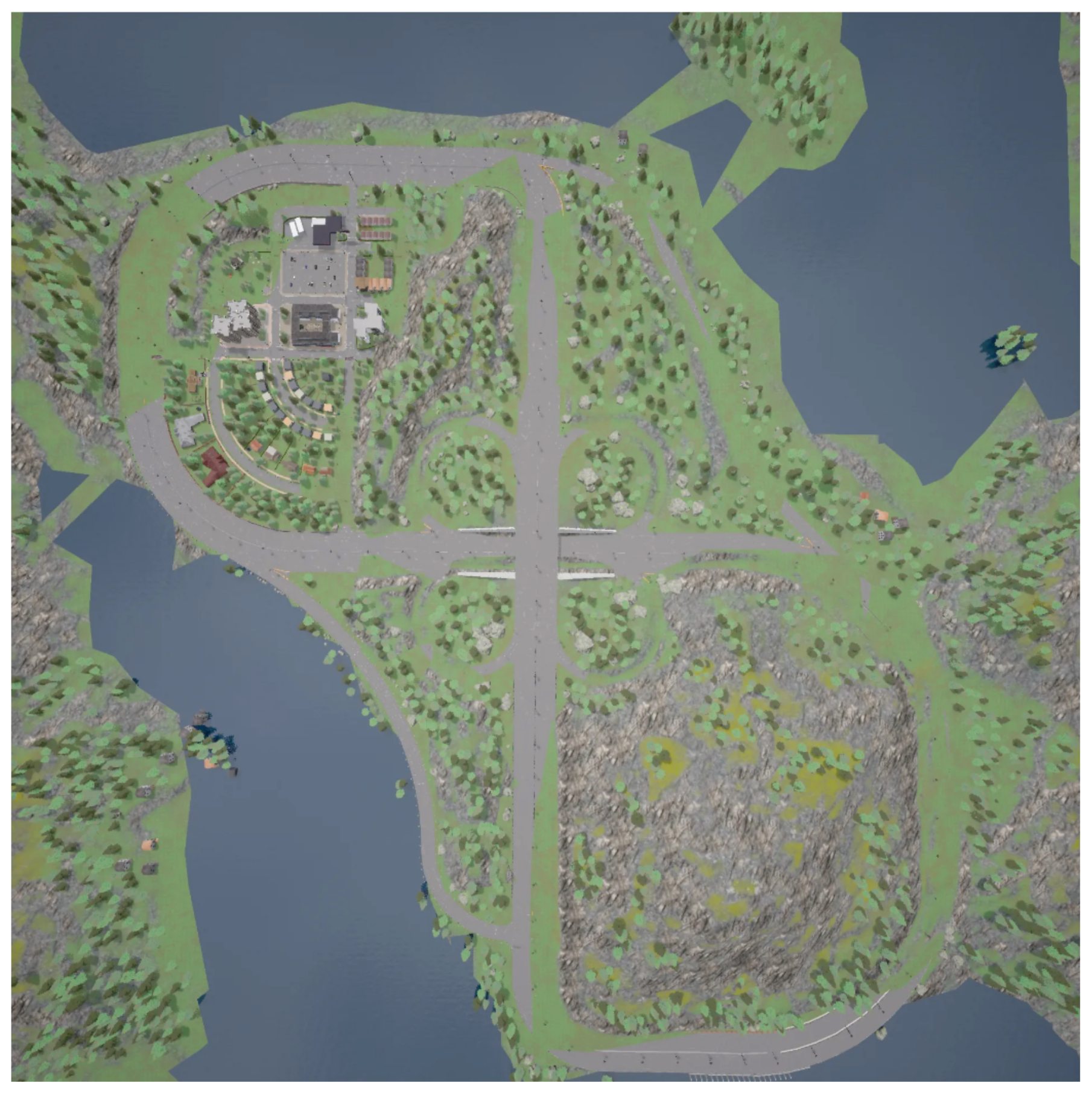
To verify the superiority and reliability of our algorithm, we performed additional validation in a 3D scene. We simulated realistic scenarios using the CARLA [33] simulator. This open-source autonomous driving simulator was built from scratch as a modular and flexible API to solve various tasks involved in autonomous driving problems. Town 4, as shown in Figure 7, was a small town with a backdrop of snow-capped mountains and conifers. As seen in Figure 8, a multi-lane road circumnavigated the town. The road network consisted of a small network of short streets and junctions between commercial and residential buildings, with a “figure-eight-shaped”-style ring road circumnavigating the buildings and a nearby mountain. The crossing of the road was designed as an underpass/overpass with circular slip roads.
In our task setup, our objective was to maximize the effective distance traveled by the vehicle agent within a fixed 1000 environment steps. The metrics for evaluating the performance of this task were the driving distance and reward. The greater the driving distance and reward, the better the model was considered to have performed. Further hyperparameters are described in Table 1.

5. Results

5.1. Results for Highway_Env

5.1.1. Rewards

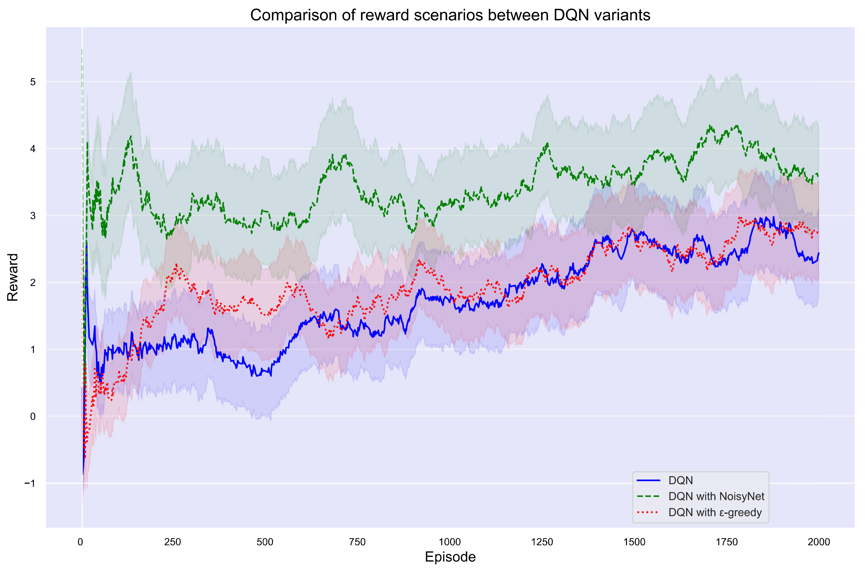
We analyzed the reward values from 2000 episodes collected across three experimental sets. After averaging these values, we applied a smoothing technique to the data and plotted the resulting curves. The reward comparison graphs (Figure 9 and Figure 10) revealed important insights into the performances of the different DQN and DDQN variants across episodes. In Figure 9, the DQN with NoisyNet clearly outperformed both the standard DQN and DQN with ϵ -greedy, which highlighted the effectiveness of NoisyNet in enhancing the exploration and achieving higher rewards. The ϵ -greedy variant showed some improvement over the standard DQN, but it did not reach the level of performance seen with NoisyNet. In contrast, Figure 10 shows that while the DDQN with NoisyNet initially performed well, the standard DDQN eventually surpassed it as the training progressed. This suggests that although NoisyNet provided early benefits, the standard DDQN may offer better long-term stability and higher rewards. The DDQN with the ϵ -greedy variant demonstrated more consistent performance than NoisyNet but still fell short of the standard DDQN. These figures collectively underscored the complex dynamics of exploration strategies in reinforcement learning, with NoisyNet offering strong early performance, while the standard DDQN showed superior long-term results in certain cases.
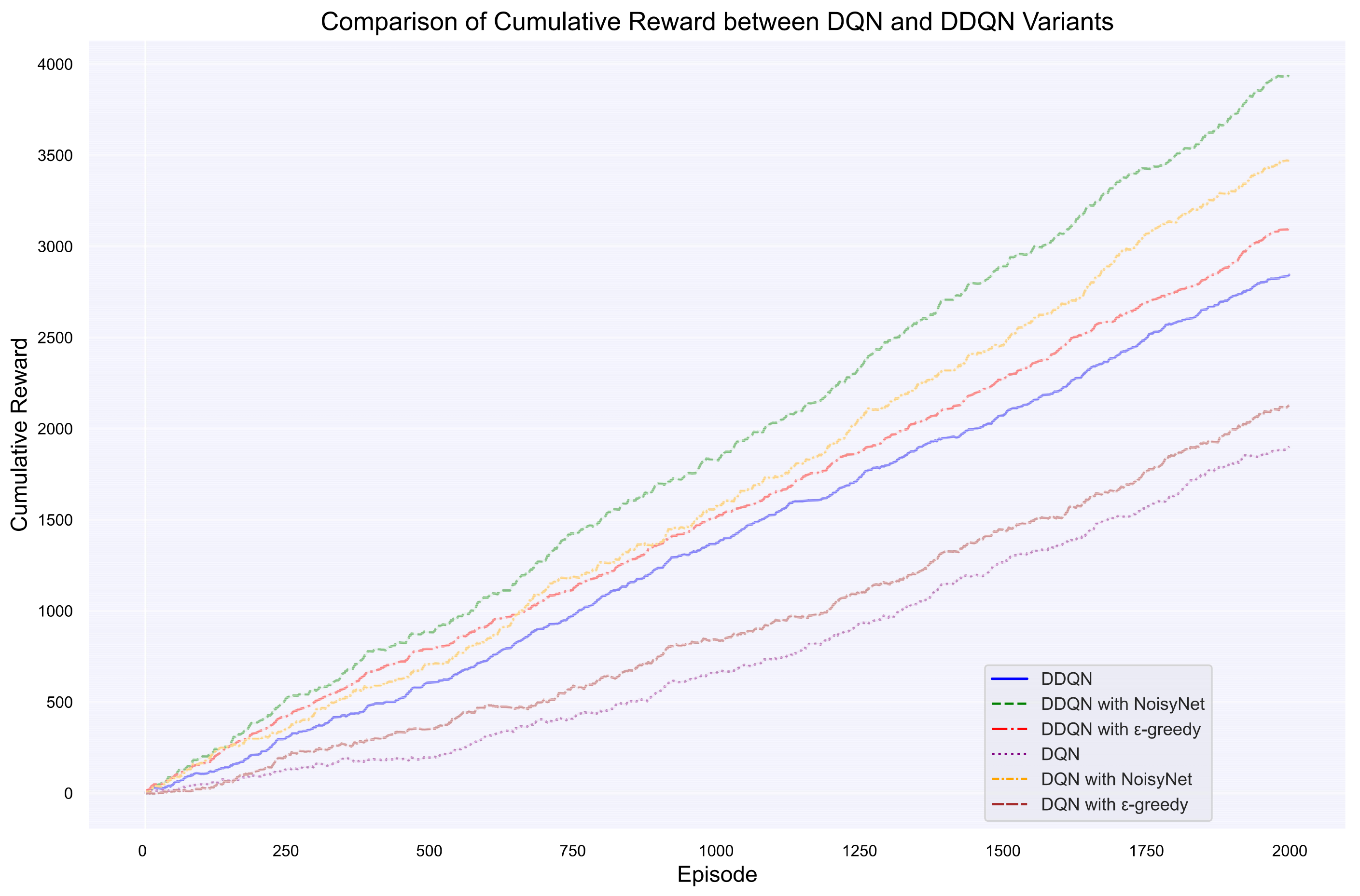
The cumulative rewards graph (Figure 11) clearly illustrates the significant differences in performance between various DQN and DDQN variants. The combination of DDQN with NoisyNet performed the best, where it achieved the highest cumulative rewards, thus indicating its superior ability to balance exploration and exploitation and leading to better long-term learning outcomes. While DDQN with ϵ -greedy also outperformed the standard DDQN, it did not reach the levels of the NoisyNet variant, which suggests that NoisyNet is more effective at reducing overestimation bias and enhancing learning robustness. In contrast, although DQN with NoisyNet outperformed the other DQN variants, it still fell short of the DDQN combinations, thus further highlighting the advantages of the DDQN architecture when paired with exploration strategies like NoisyNet. Overall, the combination of NoisyNet with DDQN demonstrates the most significant improvement in cumulative rewards in complex reinforcement learning tasks.
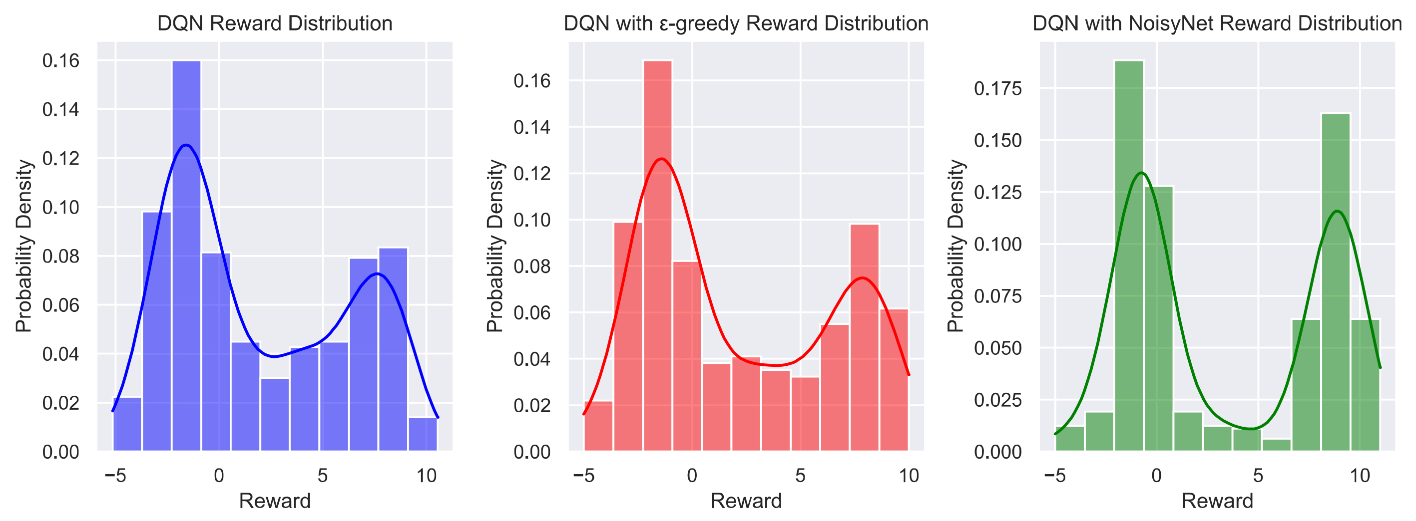
The reward distribution charts in Figure 12 reveal significant differences in how the DQN and its variants performed in terms of the reward distribution. The standard DQN shows a bimodal distribution, with the rewards mainly concentrated around 0 and close to 10. This indicates that the DQN could achieve high rewards in certain states, but overall, the reward values remained relatively low, which reflected inconsistent learning effectiveness across different states. The DQN with the ϵ -greedy strategy exhibited a more pronounced peak in the reward distribution, primarily around 0, with a noticeable spread in the positive reward range (between 5 and 10). This suggests that the ϵ -greedy strategy enhanced the DQN exploration capability, which led to a more balanced distribution of rewards, though still leaning toward lower values. In contrast, the reward distribution for the DQN with NoisyNet was more dispersed. Although the bimodal structure persisted, the reward values were more evenly spread, where they covered a range from −5 to 10. This indicates that NoisyNet significantly boosted the DQN exploration ability, which prevented rewards from being overly concentrated in a specific range, and thus, demonstrating stronger exploration capabilities and a broader reward coverage. Overall, these distribution charts clearly reflected the impact of different strategies on the DQN exploration and exploitation balance. In particular, the introduction of NoisyNet resulted in a more diversified reward distribution, which highlighted its advantages in enhancing the learning performance.
The analysis of the reward distribution charts in Figure 13 indicates that the DDQN and DDQN with ϵ -greedy exhibited more concentrated reward values compared with other variants, with no occurrence of particularly low rewards. This suggests that both algorithms maintained stable performance during training, thus effectively avoiding the pitfall of extremely low rewards. This characteristic was confirmed by the reward distribution charts, where the smaller shaded areas (variance) further demonstrated the reduced reward fluctuations, thus highlighting the consistency and reliability of these algorithms. Specifically, the rewards for the DDQN and DDQN with ϵ -greedy were primarily concentrated in the mid-range. Although they failed to explore rewards above seven, they successfully avoided the trap of low reward regions. This indicates that these algorithms could effectively enhance the overall performance while maintaining relatively stable learning outcomes. However, this stability might come at the cost of exploring higher reward regions, but overall, they showed more consistent performance and reduced the risk of extremely low rewards.
NoisyNet-DDQN, on the other hand, managed to retain the advantages of DDQN and DDQN with ϵ -greedy while also effectively exploring high-value regions. Specifically, NoisyNet-DDQN not only exhibited a reward distribution similar to the other two algorithms that was characterized by stable and mid-range reward values that avoided extremely low rewards but also demonstrated a strong exploratory capability, where it more frequently reached reward regions above seven. This indicates that the random perturbation mechanism introduced by NoisyNet enhanced the diversity of exploration, thus enabling the algorithm to break out of local optima and discover and exploit higher rewards, all while maintaining the overall performance stability.

5.1.2. Success Rate

The success rate of the vehicle passage is a crucial metric that reflects the effectiveness of our models. We computed the success rates for the traditional DQN, DDQN, and our DynamicNoise-enhanced algorithms across ten experiments, and then determined their average values. The success rate for the conventional DQN was 52.8%, while the ϵ -greedy modification achieved 62.5%. The DDQN algorithm achieved a success rate of 68.6%, with the ϵ -greedy variation reaching 74.5%. Both were still significantly lower than the 88.9% success rate recorded for DQN with NoisyNet and 91.2% for DDQN with NoisyNet. The analysis of the reward distribution revealed that the rewards obtained by the algorithms using the DynamicNoise framework were mainly concentrated at higher values, thus indirectly affirming their excellent success rates and suggesting that their network architectures are more efficient.
Moreover, we analyzed the variance of the rewards for all methods across the ten data sets by computing the average values. The variance of the traditional DQN was 18.46, while the ϵ -greedy method had a variance of 19.32. In contrast, DQN with NoisyNet had a higher variance value of 23.26, and DDQN with NoisyNet showed a similar trend with a variance of 23.61, which indicates their enhanced exploratory capabilities. However, the DDQN algorithm and its ϵ -greedy variation, which is known for more conservative exploration strategies, exhibited lower variance values of 14.14 and 15.26, respectively. This lower variance reflects the DDQN-based methods’ tendency toward stability and reduced exploration compared with the more aggressive exploration in the NoisyNet-enhanced strategies. Overall, the higher variance observed in the DynamicNoiseDQN-based methods confirmed their superior exploratory capabilities, while the lower variance in the DDQN methods underscored their focus on stability and consistent performance.

5.1.3. Number of Iterations at Convergence

To further assess the task completion efficiency, we compared the minimum number of episodes required by all networks to achieve their objectives. DDQN with NoisyNet particularly stood out by requiring only 210 attempts to succeed, which was a drastic reduction from the original 1220 attempts with DQN, thus representing an improvement of 82.79%. The DDQN algorithm required 370 attempts, and its ϵ -greedy variation further improved to 290 attempts, where both were significantly fewer than the traditional DQN and its ϵ -greedy variant, which required 1240 episodes. This comparison underscored the effectiveness of integrating advanced strategies, such as NoisyNet and doubling techniques, into both the DQN and DDQN. Such enhancements not only boosted the efficiency of the learning process but also significantly increased the speed and reliability of reaching optimal solutions in dynamic environments.

5.1.4. Time for Completion of Tasks

The comparative data showcase significant advancements in the time efficiency across the various DQN configurations. From Table 2, it can be seen that the original DQN model required an average of 6.58 s per episode, which is indicative of the baseline performance. When incorporating the ε -greedy strategy, the time was slightly reduced to 6.41 s, which indicates a marginal improvement in the processing efficiency.
However, the integration of the DDQN and the DynamicNoiseDQN framework presented more notable time reductions. The standard DDQN model required 6.40 s, while the DDQN with ε -greedy strategy further reduced this to 6.25 s. The DQN with NoisyNet reduced the average time to 6.01 s, and the DDQN with NoisyNet achieved the most efficient time of 5.93 s, which represented a 10.96% improvement over the original DQN model. These results highlight the effectiveness of using NoisyNet in combination with DDQN, thus demonstrating significant improvements in both the time efficiency and overall task performance.
These results demonstrate that integrating advanced strategies, such as NoisyNet and the doubling technique, enhanced the time efficiency of the network. This reduction in time not only indicates quicker decision-making capabilities but also highlights the ability of the models to handle dynamic environments more effectively.

5.2. Result in CARLA

We report the comparison data regarding the episode distance and episode reward for the vehicle over 1000 fixed environment steps in Table 3, while the obstacle avoidance ability of the vehicle is visualized in Figure 14. The average steering control magnitude percentage per step was recorded throughout the training.
The experiments demonstrated that the proposed method, when integrated into the SAC reinforcement learning framework, could effectively enhance the driving performance of the base framework. The results obtained with the two algorithms are shown in Figure 15. Specifically, on the one hand, the proposed method (SAC + NoisyNet) achieved the optimal episode driving distance of 540.5 m, which was an improvement of nearly 18.9% compared with the 454.1 m achieved by the original SAC method (as shown in Table 3). On the other hand, as shown on the right side of the figure, the proposed method performed better in steering control, where it maintained a stable steering magnitude, thus effectively enhancing the overall driving distance. Overall, these qualitative experiments strongly proved the control performance of the proposed method in the context of autonomous driving.

6. Conclusions

We proposed the NoisyNet framework to address the slow convergence, instability, and low exploration efficiency in high-dimensional state spaces of reinforcement learning algorithms, particularly in complex driving scenarios. By introducing noise parameters, NoisyNet effectively balanced exploration and exploitation, thus enhancing decision making and adaptability. Integrated with the DQN and SAC algorithms, NoisyNet was experimentally validated, thus demonstrating significant improvements in both performance and stability. This framework shows great promise for optimizing the intelligence and reliability of autonomous driving systems by improving their ability to manage complex traffic environments, enhancing the decision-making and control efficiency, and optimizing the collaborative operation of autonomous vehicle fleets to increase the overall traffic efficiency and safety.
Despite its strong performance in laboratory settings, NoisyNet may encounter challenges when applied to real-world environments, where complexity and interference can affect its effectiveness. To address this, our future work will focus on enhancing the robustness of the framework through extensive testing on autonomous vehicles and UGVs in various real-world traffic scenarios, including urban, highway, and rural environments. We will refine NoisyNet for seamless integration with existing autonomous driving systems to ensure real-time processing and the adherence to safety standards required for deployment. Additionally, we plan to validate the performance of NoisyNet under practical conditions by collaborating with industry partners to ensure it meets the rigorous demands of real-world applications. By expanding its application to intelligent transportation systems, we aim to develop more resilient and efficient traffic management solutions, thus ultimately bridging the gap between simulation and real-world deployment.

Author Contributions

Data curation, H.S., J.C. and M.Z.; Formal analysis, J.C. and M.L.; Funding acquisition, F.Z., M.L. and M.L.; Investigation, F.Z.; Methodology, H.S., M.L. and M.Z.; Project administration, F.Z. and M.L.; Resources, H.S.; Software, H.S.; Supervision, F.Z. and M.L.; Validation, H.S.; Writing—Original draft, H.S. and J.C.; Writing—Review & editing, J.C. and M.Z. All authors have read and agreed to the published version of the manuscript.

Funding

This research was supported by the Jilin Province Transportation Science and Technology project (no. 2018ZDGC-4) and Traffic engineering AI digital assistant (NO.2024BQ0032) from JLU and JLJU.

Data Availability Statement

Dataset available on request from the authors.

Conflicts of Interest

The authors declare no conflict of interest.

Abbreviations

The following abbreviations were used in this manuscript:
RLReinforcement learning
SACSoft actor–critic
KDEKernel density estimate
DQNDeep Q-network
DDQNDouble DQN
MPCModel predictive control
PIDProportional–integral–derivative
MDPMarkov decision process
UAVUnmanned aerial vehicle

References

  1. Althoff, M.; Lutz, S. Automatic generation of safety-critical test scenarios for collision avoidance of road vehicles. In Proceedings of the 2018 IEEE Intelligent Vehicles Symposium (IV), Changshu, China, 26–30 June 2018; IEEE: Piscataway, NJ, USA, 2018; pp. 1326–1333. [Google Scholar]
  2. Gao, F.; Duan, J.; Han, Z.; He, Y. Automatic virtual test technology for intelligent driving systems considering both coverage and efficiency. IEEE Trans. Veh. Technol. 2020, 69, 14365–14376. [Google Scholar] [CrossRef]
  3. Li, Z.; Zhou, A.; Pu, J.; Yu, J. Multi-modal neural feature fusion for automatic driving through perception-aware path planning. IEEE Access 2021, 9, 142782–142794. [Google Scholar] [CrossRef]
  4. James, J.; Yu, W.; Gu, J. Online vehicle routing with neural combinatorial optimization and deep reinforcement learning. IEEE Trans. Intell. Transp. Syst. 2019, 20, 3806–3817. [Google Scholar]
  5. Zhang, Y.; Macke, W.; Cui, J.; Hornstein, S.; Urieli, D.; Stone, P. Learning a robust multiagent driving policy for traffic congestion reduction. Neural Comput. Appl. 2023, 1–14. [Google Scholar] [CrossRef]
  6. Zhu, L.; Gonder, J.; Bjarkvik, E.; Pourabdollah, M.; Lindenberg, B. An automated vehicle fuel economy benefits evaluation framework using real-world travel and traffic data. IEEE Intell. Transp. Syst. Mag. 2019, 11, 29–41. [Google Scholar] [CrossRef]
  7. Le-Anh, T.; Koster, M.D. A review of design and control of automated guided vehicle systems. Eur. J. Oper. Res. 2006, 171, 1–23. [Google Scholar] [CrossRef]
  8. Cheein, F.A.A.; Cruz, C.D.L.; Bastos, T.F.; Carelli, R. Slam-based cross-a-door solution approach for a robotic wheelchair. Int. J. Adv. Robot. Syst. 2009, 6, 20. [Google Scholar] [CrossRef]
  9. Suh, J.; Chae, H.; Yi, K. Stochastic model-predictive control for lane change decision of automated driving vehicles. IEEE Trans. Veh. Technol. 2018, 67, 4771–4782. [Google Scholar] [CrossRef]
  10. Wang, P.; Chan, C.-Y.; de La Fortelle, A. A reinforcement learning based approach for automated lane change maneuvers. In Proceedings of the 2018 IEEE Intelligent Vehicles Symposium (IV), Changshu, China, 26–30 June 2018; IEEE: Piscataway, NJ, USA, 2018; pp. 1379–1384. [Google Scholar]
  11. Aradi, S. Survey of deep reinforcement learning for motion planning of autonomous vehicles. IEEE Trans. Intell. Transp. Syst. 2020, 23, 740–759. [Google Scholar] [CrossRef]
  12. Haarnoja, T.; Zhou, A.; Hartikainen, K.; Tucker, G.; Ha, S.; Tan, J.; Kumar, V.; Zhu, H.; Gupta, A.; Abbeel, P.; et al. Soft actor-critic algorithms and applications. arXiv 2018, arXiv:1812.05905. [Google Scholar]
  13. Li, J.; Chen, Y.; Zhao, X.; Huang, J. An improved dqn path planning algorithm. J. Supercomput. 2022, 78, 616–639. [Google Scholar] [CrossRef]
  14. Alizadeh, A.; Moghadam, M.; Bicer, Y.; Ure, N.K.; Yavas, U.; Kurtulus, C. Automated lane change decision-making using deep reinforcement learning in dynamic and uncertain highway environments. In Proceedings of the 2019 IEEE Intelligent Transportation Systems Conference (ITSC), Auckland, New Zealand, 27–30 October 2019; pp. 1399–1404. [Google Scholar]
  15. Van Hasselt, H.; Guez, A.; Silver, D. Deep reinforcement learning with double q-learning. In Proceedings of the AAAI Conference on Artificial Intelligence, Phoenix, AZ, USA, 12–17 February 2016; Volume 30. [Google Scholar]
  16. Liao, J.; Liu, T.; Tang, X.; Mu, X.; Huang, B.; Cao, D. Decision-making strategy on the highway for autonomous vehicles using deep reinforcement learning. IEEE Access 2020, 8, 177804–177814. [Google Scholar] [CrossRef]
  17. Seong, H.; Jung, C.; Lee, S.; Shim, D.H. Learning to drive at unsignalized intersections using attention-based deep reinforcement learning. In Proceedings of the 2021 IEEE International Intelligent Transportation Systems Conference (ITSC), Indianapolis, IN, USA, 19–22 September 2021; pp. 559–566. [Google Scholar]
  18. Lillicrap, T.P.; Hunt, J.J.; Pritzel, A.; Heess, N.; Erez, T.; Tassa, Y.; Wierstra, D. Continuous control with deep reinforcement learning. arXiv 2015, arXiv:1509.02971. [Google Scholar]
  19. Schulman, J.; Wolski, F.; Dhariwal, P.; Radford, A.; Klimov, O. Proximal policy optimization algorithms. arXiv 2017, arXiv:1707.06347. [Google Scholar]
  20. Chen, D.; Jiang, L.; Wang, Y.; Li, Z. Autonomous driving using safe reinforcement learning by incorporating a regret-based human lane-changing decision model. In Proceedings of the 2020 American Control Conference (ACC), Denver, CO, USA, 1–3 July 2020; IEEE: Piscataway, NJ, USA, 2020; pp. 4355–4361. [Google Scholar]
  21. He, X.; Yang, H.; Hu, Z.; Lv, C. Robust lane change decision making for autonomous vehicles: An observation adversarial reinforcement learning approach. IEEE Trans. Intell. Veh. 2022, 8, 184–193. [Google Scholar] [CrossRef]
  22. Li, G.; Yang, Y.; Li, S.; Qu, X.; Lyu, N.; Li, S.E. Decision making of autonomous vehicles in lane change scenarios: Deep reinforcement learning approaches with risk awareness. Transp. Res. Part C Emerg. Technol. 2022, 134, 103452. [Google Scholar] [CrossRef]
  23. Peng, J.; Zhang, S.; Zhou, Y.; Li, Z. An integrated model for autonomous speed and lane change decision-making based on deep reinforcement learning. IEEE Trans. Intell. Transp. Syst. 2022, 23, 21848–21860. [Google Scholar] [CrossRef]
  24. Hoel, C.-J.; Tram, T.; Sjöberg, J. Reinforcement learning with uncertainty estimation for tactical decision-making in intersections. In Proceedings of the 2020 IEEE 23rd International Conference on Intelligent Transportation Systems (ITSC), Rhodes, Greece, 20–23 September 2020; IEEE: Piscataway, NJ, USA, 2020; pp. 1–7. [Google Scholar]
  25. Zhang, C.; Kacem, K.; Hinz, G.; Knoll, A. Safe and rule-aware deep reinforcement learning for autonomous driving at intersections. In Proceedings of the 2022 IEEE 25th International Conference on Intelligent Transportation Systems (ITSC), Macau, China, 8–12 October 2022; IEEE: Piscataway, NJ, USA, 2022; pp. 2708–2715. [Google Scholar]
  26. Chen, L.; Hu, X.; Tang, B.; Cheng, Y. Conditional dqn-based motion planning with fuzzy logic for autonomous driving. IEEE Trans. Intell. Transp. Syst. 2020, 23, 2966–2977. [Google Scholar] [CrossRef]
  27. Li, G.; Li, S.; Li, S.; Qin, Y.; Cao, D.; Qu, X.; Cheng, B. Deep reinforcement learning enabled decision-making for autonomous driving at intersections. Automot. Innov. 2020, 3, 374–385. [Google Scholar] [CrossRef]
  28. Wu, Y.; Tucker, G.; Nachum, O. Behavior regularized offline reinforcement learning. arXiv 2019, arXiv:1911.11361. [Google Scholar]
  29. Kim, H.; Wan, W.; Hovakimyan, N.; Sha, L.; Voulgaris, P. Robust vehicle lane keeping control with networked proactive adaptation. Artif. Intell. 2023, 325, 104020. [Google Scholar] [CrossRef]
  30. Yang, J.; Kim, H.; Wan, W.; Hovakimyan, N.; Vorobeychik, Y. Certified robust control under adversarial perturbations. In Proceedings of the 2023 American Control Conference (ACC), San Diego, CA, USA, 31 May–2 June 2023; IEEE: Piscataway, NJ, USA, 2023; pp. 4090–4095. [Google Scholar]
  31. Plappert, M.; Houthooft, R.; Dhariwal, P.; Sidor, S.; Chen, R.Y.; Chen, X.; Asfour, T.; Abbeel, P.; Andrychowicz, M. Parameter space noise for exploration. arXiv 2017, arXiv:1706.01905. [Google Scholar]
  32. Leurent, E. An Environment for Autonomous Driving Decision-Making. 2018. Available online: https://github.com/eleurent/highway-env (accessed on 29 March 2024).
  33. Dosovitskiy, A.; Ros, G.; Codevilla, F.; Lopez, A.; Koltun, V. CARLA: An open urban driving simulator. In Proceedings of the 1st Annual Conference on Robot Learning, Mountain View, CA, USA, 13–15 November 2017; pp. 1–16. [Google Scholar]
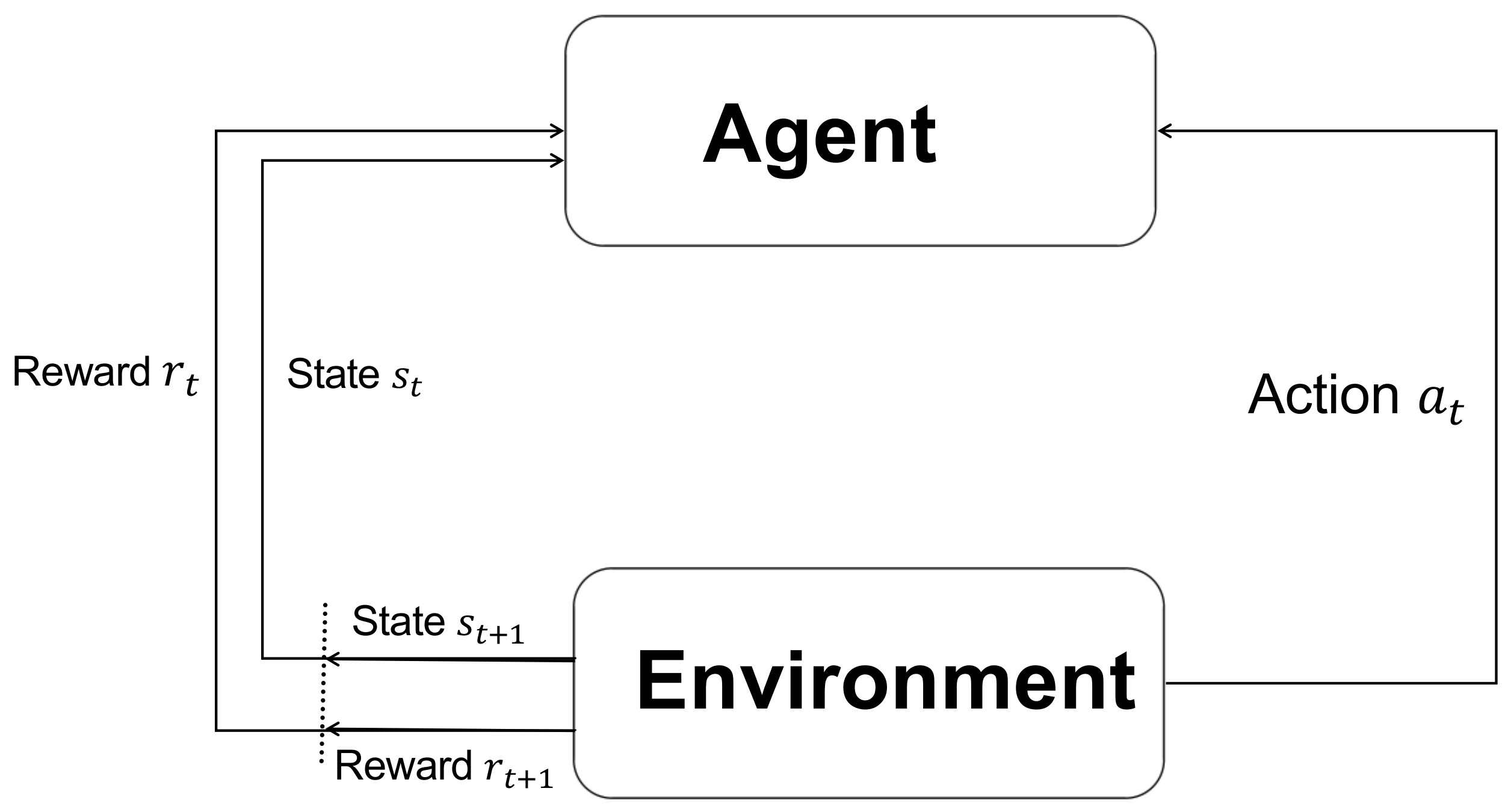
Figure 1. MDP flow diagram.
Drones 08 00470 g001
Figure 2. Schematic diagram of how the model works.
Drones 08 00470 g002
Figure 6. Environment in highway_env showing the initial state, the collision state, and the passage state.
Drones 08 00470 g006
Figure 7. Overhead view of Town 4. A multi-lane road circumnavigates the town in a figure-eight shape.
Drones 08 00470 g007
Figure 8. The network also featured an underpass and overpass with circular slip roads.
Drones 08 00470 g008
Figure 9. Comparison of reward scenarios between DQN, DQN with ε -greedy, and DQN with NoisyNet.
Drones 08 00470 g009
Figure 10. Comparison of reward scenarios between DDQN, DDQN with ε -greedy, and DDQN with NoisyNet.
Drones 08 00470 g010
Figure 11. Cumulative rewards across episodes for different DQN and DDQN variants.
Drones 08 00470 g011
Figure 12. Reward distribution of DQN, DQN with ε -greedy, and DQN with NoisyNet.
Drones 08 00470 g012
Figure 13. Reward distribution of DDQN, DDQN with ε -greedy, and DDQN with NoisyNet.
Drones 08 00470 g013
Figure 14. The red car in the middle represents the agent. This sequence of observations indicates that the algorithm could effectively avoid other cars and complete the driving task.
Drones 08 00470 g014
Figure 15. Comparison of performance metrics in CARLA autonomous driving.
Drones 08 00470 g015
Table 1. Key hyperparameters used in training stage.
HyperparameterValue
Camera number3
Full FOV angles 3 × 60 degrees
Observation downsampling 84 × 252
Initial exploration steps100
Training frames500,000
Replay buffer capacity30,000
Batch size64
Action repeat4
Stacked frames3
Δ t0.05 s
C i 0.0001
C s 1.0
Learning rate0.0005
OptimizerAdam
Table 2. Experimental results for DQN variants.
RewardSuccess RateMinimum Number of Times to CompleteTime for Completion of Tasks
DQN2.6252.8%12206.58 s
DQN with ε -greedy3.0562.5%12406.41 s
DQN with NoisyNet3.7288.9%2406.01 s
DDQN2.8568.6%3706.40 s
DDQN with ε -greedy3.1774.5%2906.25 s
DDQN with NoisyNet4.1291.2%2105.93 s
Improvement57.25%72.73%82.79%10.96%
Table 3. Comparison of performance metrics in CARLA autonomous driving evaluation.
MethodsDistanceEval RewardSteer (%)
SAC454.1 ± 13.692.9 ± 7.022.4 ± 1.3
SAC + NoisyNet (ours)540.5 ± 2.7115.8 ± 1.516.6 ± 2.0
Disclaimer/Publisher’s Note: The statements, opinions and data contained in all publications are solely those of the individual author(s) and contributor(s) and not of MDPI and/or the editor(s). MDPI and/or the editor(s) disclaim responsibility for any injury to people or property resulting from any ideas, methods, instructions or products referred to in the content.