Article

Internet of Things Based Digital Twin Model Construction and Online Fault-Tolerant Control of Hypersonic Flight Vehicle

1
Xi’an Research Institute of High-Tech, Xi’an 710025, China
2
Xi’an Institute of Microelectronics Technology, Xi’an 710065, China
3
School of Automation, Northwestern Polytechnical University, Xi’an 710072, China
*
Author to whom correspondence should be addressed.
Drones 2024, 8(9), 460; https://doi.org/10.3390/drones8090460
Submission received: 22 July 2024 / Revised: 16 August 2024 / Accepted: 23 August 2024 / Published: 4 September 2024
(This article belongs to the Section Drone Design and Development)

Abstract

:
This paper proposes a novel framework for the online fault-tolerant control of hypersonic flight vehicles (HFV). The framework contains two steps. Firstly, based on the Internet of Things (IoT) and digital twin (DT) technology, a hypersonic flight vehicle digital twin (HFVDT) model is constructed. This HFVDT model can represent the real model and the parameter changes in HFV in real-time, and can update itself by the designed updating law through the flight data acquired by IoT. Then, the model changes caused by a fault can be fed back in real-time. Based on the real-time model, a model predictive static programming (MPSP) based controller design method is proposed to solve the online fault-tolerant control problem of HFV. MPSP provides a feasible online solution to optimal control problems with constraints. By converting the nonlinear optimal control problem to a static optimization the problem, the quantity of computation is greatly reduced, and then the optimal can be solved online. By the HFVDT and MPSP framework, the model change can be monitored and then an optimal controller can be constructed in real time. In this case, the fault-tolerant control problem of HFV can solved and the tracking performance is guaranteed. Finally, the novel framework is carried out on a numeral simulation to show its effectiveness.

1. Introduction

A hypersonic flight vehicle (HFV) is a typical multi-purpose aircraft and has driven much attention in recent years. Because of the strong coupling between the scramjet engine and flight dynamics, the modeling and controller design for HFV is challenging and is a hot topic nowadays [1].
A complex nonlinear model, which contains the flexible states of HFV is widely utilized [2]. Based on this exact HFV model, linear [3] and nonlinear controllers [4] have been proposed. The backstepping controller [5] and sliding mode controller [6] has also been applied and the controller performance is acceptable. But just as listed in [7], the the pneumatic model obtained by the wind tunnel experiment is not so accurate, so model uncertainty and unmodeled dynamics are inevitable. This question has been a broad consensus and robust control has also been widely researched, such as the Takagi–Sugeno (T-S) fuzzy-based robust controller [8], LPV [9], Neural Network(NN) [6,10] and model predictive control [11] based robust controller. But almost all robust controllers have an important assumption that the uncertain and unmodeled dynamics of HFV are bounded, and although the exact model of uncertain and unmodeled dynamics is unknown, their boundary is known. Based on this assumption, the robust controller is constructed to guarantee the stability of HFV among the known boundaries. This assumption is unreasonable since the boundary of HFV’s parameters is usually unknown, and when the robust controller is committed to guaranteeing the large range stability of HFV under an unknown boundary, the tracking precision would be certainly reduced.
For the robust controller design of HFV, some research results assume that, the model of HFV is completely unknown, and then NN [12] or Fuzzy Logical System (FLS) [13] based online approach technology are utilized to identify it, NN and FLS mode based controllers are consequently proposed. This is also unreasonable since the model structure of HFV is certainly known, and what one does not know is just the specific aerodynamic coefficient. If the aerodynamic coefficient can be constructed online, the exact model of HFV is then the best model for controller design.
Because of the complicated flight environment, aircraft body injuries are inevitable for HFV; the control performance will be affected. A Conventional Fault Tolerant Controller (FTC) assumes that the model of the fault HFV is already known, or the boundary of the unknown parameter caused by the fault is known, then an active FTC controller is designed [14,15]. These FTC methods cannot achieve perfect control performance since the system model is not so exact. If the exact mode of HFV can be established online, and the FTC controller can also be designed based on the exact mode online, the FTC controller is more suitable. Unfortunately, almost all the controller design methods are designed offline and used online. When the nonlinear mode of HFV is built online, these controller design methods are out of service. In this case, an online identified method for HFV and an online controller design method are needed for the exact tracking control of HFV.
Digital twin (DT) is an exact digital model of a real system [16]. By DT, one can build the digital model of HFV, and the HFV digital model will updated online, then one can obtain the exact model of HFV in real-time [17]. If the DT of HFV can be built, the digital model is the most suitable mode for controller design. The construction of DT requires real-time flight data of HFV, so the measurement, collection and transmission of flight data is very important. IoT can provide a low latency, high reliability, security, and privacy data acquisition and transmission mechanism, and can be connected with various sensors to realize real-time data acquisition of different styles and different sampling periods, so it has been utilized for industrial systems [18,19], and the IoT-based control issues have received a lot of attention from researchers [20]. DT has been utilized in industrial automation [21], fault diagnosis [22], and decision support systems [23]. The elements of building a DT for a real system are as follows: the measurable information of the real system; the information that needs to be reconstructed in the DT model, and the reconstruction strategy. Then, for the construction of DT for HFV, one should know the sensitive devices and the relationship of signal transmission in HFV. By IoT, the DT of HFV can be constructed, and then after obtaining a DT of HFV, an online controller design method is needed.
Combining the philosophies of approximate dynamic programming (ADP) and model predictive control (MPC) [24], model predictive static programming (MPSP) is presented as an optimal controller design method under hard constraints [25]. MPSP provides a solution to optimization problems with nonlinear plant dynamics and satisfies the terminal constraints. The key idea of MPSP is converting the nonlinear optimal control problem to a static optimization problem. Control variables are the only optimizing variables, resulting in a reduction in problem size. In addition, recursive computation of the sensitivity matrices is computationally very efficient. Over the last decade, MPSP has been modified to include variability in the final time [26], tracking problems [27], controller design with uncertainty in time-invariant system parameters and initial conditions [28], and the impulsive nature of the control action [29]. The MPSP technique has also been applied to a host of challenging problems, such as missile guidance [30,31], re-entry guidance [32], mobile robotics [27], and lunar soft landing [33]. The computing quantity of MPSP is accepted as small and has the potential for online application. When the initial control value of HFV is given in place, MPSP will converge rapidly. Since the aerodynamic coefficient of HFV by wind tunnel experiments is known, an initial controller can be designed, and MPSP can converge rapidly. In this case, MPSP can be utilized for online controller design.
Based on the above discussion, a novel online model and controller designing method are proposed. IoT and DT are adopted to build the exact model of HFV online, and then MPSP is utilized to design an online controller. For constructing the HFVDT, the measurable states are all analyzed based on the actual structure and composition of HFV and are transmitted via IOT. Then, an updated strategy is designed to guarantee the correctness of the DT model. Based on the DT model of HFV, the MPSP method is listed and an MPSP-based controller updated method is designed. Then, the controller can be updated online according to the updated DT model in real-time. The main contributions of the paper are summarized as follows:
(1)
A novel framework for the online controller design of HFV is proposed. Based on this framework, the controller can be updated in real-time according to the exact model of HFV.
(2)
An IoT-based DT model is built for HFV. The measurable states of HFV are listed and the reconstruction strategy of DT is designed. Based on the measurable states and reconstruct strategy, HFVDT can approach the exact model of HFV in real time.
(3)
An online reconstructed MPSP controller is designed for HFV. Based on the proposed controller design method, an FTC controller can be reconstructed online according to the exact model of HFV, then the controller performance is improved.

2. Problem Formulation

2.1. Nonlinear Dynamics

The nonlinear model of HFV is listed as follows:
h ˙ = V sin θ α V ˙ = 1 m T cos α D g sin θ α α ˙ = 1 m V T sin α L + Q + g V cos θ α θ ˙ = Q Q ˙ = M I y y + ψ 1 η ¨ 1 I y y + ψ 2 η ¨ 2 I y y η ¨ 1 = 2 ς 1 ω 1 η ˙ 1 ω 1 2 η 1 + N 1 ψ 1 M I y y ψ 1 ψ 2 η ¨ 2 I y y η ¨ 2 = 2 ς 2 ω 2 η ˙ 2 ω 2 2 η 2 + N 2 ψ 2 M I y y ψ 1 ψ 2 η ¨ 1 I y y ,
L 1 2 ρ V 2 S C L ( α , δ e ) D 1 2 ρ V 2 S C D ( α , δ e ) M z T T + 1 2 ρ V 2 S c ¯ ( C M , α ( α ) + C M , δ e ( δ e ) ) T C T α 3 α 3 + C T α 2 α 2 + C T α α + C T 0 N 1 N 1 α 2 α 2 + N 1 α α + N 1 0 N 2 N 2 α 2 α 2 + N 2 α α + N 2 δ e δ e + N 2 0 ,
and
ρ = ρ 0 exp ( ( h h 0 ) h s ) C L = C L α α + C L δ e δ e + C L 0 C D = C D α 2 α 2 + C D α α + C D δ e 2 δ e 2 + C D δ e δ e + C D 0 C M , α = C M , α α 2 α 2 + C M , α α α + C M , α 0 C M , δ e = c e δ e , q ¯ = 1 2 ρ V 2 C T α 3 = β 1 Φ + β 2 C T α 2 = β 3 Φ + β 4 C T α = β 5 Φ + β 6 C T 0 = β 7 Φ + β 8 .
C D , C L and C M are the drag coefficient, lift coefficient and drag coefficient, respectively, C T is the coefficient in T. u = [ Φ , δ e ] T is the input of the plant. This model contains nine state variables, that is, h , V , α , θ , Q , η 1 , η ˙ 1 , η 2 , η ˙ 2 . The control inputs Φ and δ e do not occur explicitly in the equations of general longitudinal dynamics for the HFV model in (1); however, they appear through the forces and moments T, L, D, M, N 1 and N 2 .

2.2. Fault of HFV and Control Objective

In this paper, the FTC control of HFV is considered. In most literature, the fault of HFV is the loss of efficiency, such as
u r = ρ u c
where u c is the control command computed by the onboard computer of HFV and u r are the real control inputs that HFV can provide, and ρ is the rate of failure. In FTC design, ρ is assumed to be known or at least the boundary of ρ is known.
The above expression is not so reasonable, since when the efficiency of the control input is lost, such as the air rudder being damaged, the aerodynamic coefficient of HFV will all be changed. More specifically, the lift coefficient C L , the drag coefficient C D , moment coefficient C M will all change according to the damage to the air rudder δ e . In this case, only assuming that the rudder surface of the vehicle has a fault is unreasonable. But if the damage of C L , the drag coefficient C D , moment coefficient C M are all taken into account, the aerodynamic model of the damage should be rebuilt for controller design. In a real flight environment, the damaged aerodynamic model is difficult to obtain.
In this paper, a novel framework for the FTC of HFV is proposed. By DT, the real value of the lift coefficient C L , the drag coefficient C D , the moment coefficient C M can be obtained in real-time, and then by designing a controller online according to the HFVDT model, the FTC control performance will certainly be improved. Then, the main objectives of this paper are as follows:
(1)
Constructing a DT model for HFV in this HFVDT model, the aerodynamic coefficient can be updated in real-time according to the flight date of HFV;
(2)
Designing an online controller for HFVDT, and the designed controller can guarantee the controller performance by a small computing quantity.

3. IoT-Based Digital Twin Model Construction

In this section, the construction of HFVDT is discussed and the updating law of HFVDT is proposed. By the designed parameter updating law, HFVDT can approach the real model of HFV online.
The design of the DT can be divided into many levels but for the controller design, the functional level DT mode of the HFV is suitable. Considering the requirements for establishing a digital twin, the building step can be divided into the following steps: (1) determining the form of the established digital twin; (2) finding the measurable states of the actual physical system; (3) finding the interaction information between the digital twin and the actual physical system; (4) designing the updating law for calculating digital models.
According to the above requirements, combined with the design requirements of the HFV control system, the functional digital twin of HFV should have the following form: (1) The established functional digital twin should be able to reflect the actual aerodynamic coefficient of HFV in real time; (2) The established functional digital twin should be able to reflect the actual working status of the aircraft actuator in real time; (3) the established functional digital twin can complete the parameter update of the functional digital twin according to the measurable flight status information of the aircraft.

3.1. Measurable Physical States

In practice, the acceleration of a flight vehicle can be measured by an accelerometer, and the flight angular velocity of a flight vehicle also can be measured by a gyroscope. Then, the aircraft’s angular velocity and apparent acceleration can be obtained in real-time. According to the navigation calculation, it can be known that the real-time attitude, quality and apparent acceleration of the flight aircraft can be obtained in real-time so that the resultant force and moment of the aircraft are real-time calculable. Then, the real-time lift, drag, side force and pitch moment, yaw moment and roll moment of the aircraft can be calculated.
 Assumption A1. 
It should be noted that in the equilibrium state, the aerodynamic moment of the aircraft is 0, but the control torque of the aircraft will not be 0 when the aircraft is maneuvering or the fault occurred.
Therefore, in the functional digital twin modeling of HFV, the measurable/computable quantities obtained by the physical entities of the aircraft can be summarized as (1) Aerodynamic force and torque of the aircraft; (2) the attitude angle of the aircraft; (3) Status information of the aircraft, including the speed and altitude of the aircraft
Rewrite the lift coefficient C L , the drag coefficient C D , the moment coefficient C M
L = 1 2 ρ V 2 S C L α α + C L δ e δ e + C L 0 D = 1 2 ρ V 2 S C D α 2 α 2 + C D α α + C D δ e 2 δ e 2 + C D δ e δ e + C D 0 M = z T T + 1 2 ρ V 2 S c ¯ ( C M , α α 2 α 2 + C M , α α α + C M , α 0 + c e δ e )
in the above equation, the measurable and computed states are as follows: L , D , M , ρ , V , S , z T , T , c ¯ , α , δ e , then the above equation can be rewritten as:
C L α α + C L δ e δ e + C L 0 = 2 L ρ V 2 S C D α 2 α 2 + C D α α + C D δ e 2 δ e 2 + C D δ e δ e + C D 0 = 2 D ρ V 2 S C M , α α 2 α 2 + C M , α α α + C M , α 0 + c e δ e = 2 M 2 z T T ρ V 2 S c ¯
For the above equation, what one needs to determine is the aerodynamic coefficient. The above equations are multi-variable differential equations, but when HFV are flighting, the measurable states α and δ e are changing all the time, so the above multi-variable differential equations are solvable.
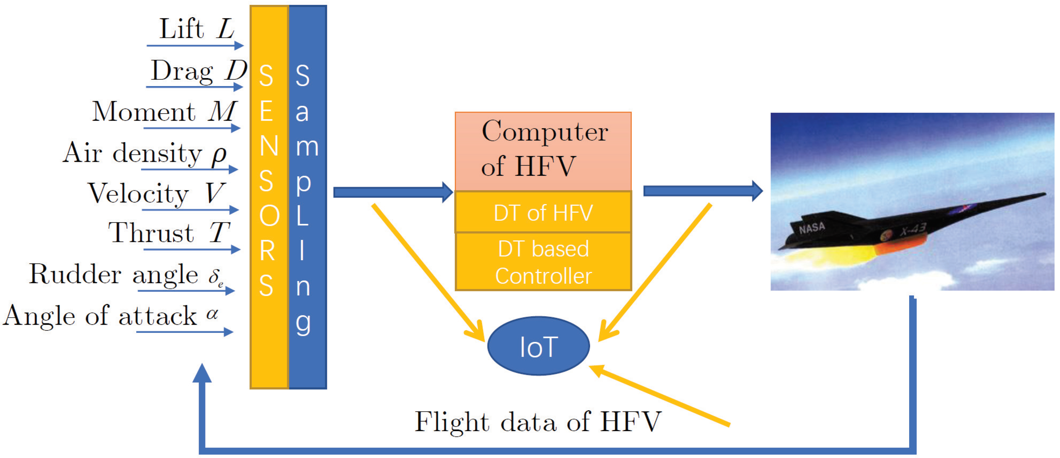
Figure 1 shows the basic principle of constructing the DT model of HFV. Firstly, the accelerometer of HFV measures the acceleration of HFV, so as to obtain the resultant force on HFV. Then, the rate gyro measures the flight angle information and determines the real-time attitude of HFV. Finally, the thrust of HFV is determined by the propellant mass consumption of the engine. The L , D , and M of HFV are obtained by combining the three, and the aerodynamic coefficient of HFV is obtained by reverse calculation.

3.2. IoT-Based Flight Data Collection and Transmission

Just as mentioned in the above subsection, the measurable physical states are complex, and in practice, the measurable physical states include voltage, current, displacement, angle, speed, and so on. How to monitor them in real-time and transmit them effectively is the basis and key for building digital twin models of HFV. IoT can connect resources and collect data about the physical world, so IoT is utilized here.
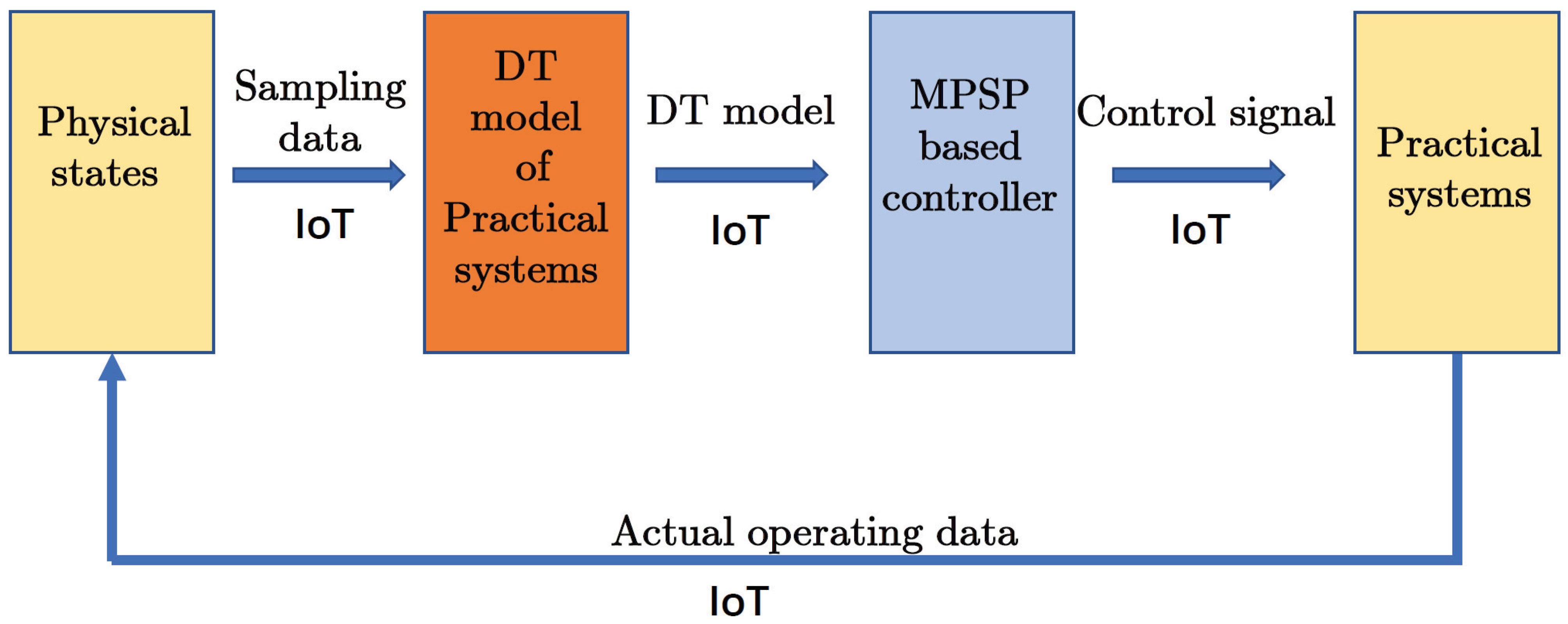
The IoT-based flight data collection and transmission framework is given in Figure 2. Figure 2 shows that the measurable physical states of HFV are all collected by IoT through different sensors, and that they are all transmitted to the computer of HFV. In the computer, the DT model of HFV is constructed in real-time based on the real-time data and modeling method which will be discussed in the next subsection. Then, new control commands are generated and applied to control HFV. So, in the whole control loop, IoT is a collection center and transmission link for information.

3.3. HFVDT Constructing Method

In the above subsection, the measurable states and the data transfer method for constructing HFVDT have been summarized. In this subsection, the constructing method for HFVDT is discussed.
In the expression of lift L, there are three unknown parameters that need to be computed by the measurable states. More specially, C L α , C L δ e , C L 0 need to be computed by L , ρ , V , S , α , δ e . It is assumed that the failure of the aircraft is a slow variable or a constant, that is, the above parameters are refrigeration variable or constant. Therefore, if the computer of HFV can continuously receive the angle of attack α , air rudder δ e and other measurable signals of HFV, the specific value of the lift coefficient of the aircraft can be deduced in reverse. To be specific, the DT algorithm for the aerodynamic coefficient of lift L is as follows:
DT Algorithm for L
f o r i = 1 : n ( n 3 )
Step 1 : receiving the value of h , V , α , δ e ,
computing the value of 2 L ρ V 2 S , marked as ϝ L i = 2 L i ρ i V i 2 S , χ L i = α i , δ e i , 1
Step 2: 2 : utilizing the eqaution ϝ L i = χ L i C L D T T , where C L D T = C L α , C L δ e , C L 0
then ϝ L = ϝ L 1 ϝ L 2 ϝ L 3 = χ L C L D T T = χ L 1 χ L 2 χ L 3 C L D T T , obtaining the value of C L D T T ,
C L D T T = χ L T ϝ L
end
Similar to the computing method of C L , the constructing method of C D and C M are
DT Algorithm for D
f o r i = 1 : n ( n 5 )
Step 1 : receiving the value of h , V , α , δ e ,
computing the value of 2 D ρ V 2 S , marked as ϝ D i = 2 D i ρ i V i 2 S , χ D i = α i 2 , α i , δ e i 2 , δ e i , 1
Step 2: utilizing the eqaution ϝ D i = χ D i C D D T T , where C D D T = C D α 2 , C D α , C D δ e 2 , C D δ e , C D 0
then ϝ D = ϝ D 1 ϝ D 2 ϝ D 3 ϝ D 4 ϝ D 5 = χ D C D D T T = χ D 1 χ D 2 χ D 3 χ D 4 χ D 5 C D D T T , obtaining the value of C D D T T ,
C D D T T = χ D T ϝ D
end
DT Algorithm for M
f o r i = 1 : n ( n 4 )
Step 1 : receiving the value of h , V , α , δ e ,
computing the value of 2 M ρ V 2 S , marked as ϝ M i = 2 M i ρ i V i 2 S , χ M i = α i 2 , α i , δ e i , 1
Step 2: utilizing the eqaution ϝ M i = χ M i C M D T T , where C M D T = C M , α α 2 , C M , α α , c e , C M , α 0
then ϝ M = ϝ M 1 ϝ M 2 ϝ M 3 ϝ M 4 = χ M C M D T T = χ M 1 χ M 2 χ M 3 χ M 4 C M D T T , obtaining the value of C M D T T ,
C M D T T = χ M T ϝ M
end
 Remark 1. 
From the above algorithm, the real value of aerodynamic coefficient L, D, M can be computed online. The calculated amounts are also accepted. Then the HFVDT can be constructed.
 Remark 2. 
In the real flight process, the changing speed of α and δ e may be very small, so the solution of algorithms L, D and M is a singularity, then the computed value of aerodynamic coefficient L, D, M are wrong. As long as enough data can be collected, and by least squares fitting, this effect will be minimized.

4. MPSP-Based Controller Design

After obtaining the HFVDT, the real model of HFV is built, and then an online controller-designed method is needed for the real-time model. MPSP is a controller design method with online applications; in this paper, MPSP is utilized for the online controller design.
By submitting (2) and (3) to (1), (1) can be transformed into a normal form:
x ˙ = F ( x , u ) ,
where x = [ h , V , α , θ , Q , η 1 , η ˙ 1 , η 2 , η ˙ 2 ] T , u = [ Φ , δ e ] T , the details of F ( x , u ) can be found in [13]. Then, the theoretical details of MPSP are performed.

4.1. Constructing Method of MPSP

The design objective is to find an appropriate control vector u k ( k = 1 , 2 , , N 1 ) , which starts from an initial guess, and derive the output Y N reaches the desired value Y N * at the final time step, Y N Y N * , and the control cost function should also be take into account. The final output error is defined as Δ Y N = Y N * Y N , then Taylor series expansion is utilized by neglecting higher-order terms, then the error in the output can be expressed as
Δ Y N d Y N = Y N X N d X N
Considering the nonlinear model of the control system, the error (8) in state at time step (k + 1) can be rewritten as
d X k + 1 = F k X k d X k + F k U k d u k
where d X k and d u k are the error of state and control at time step k, respectively. Let k = N 1 , one can obtain
d Y N = Y N X N F N 1 X N 1 d X N 1 + F N 1 U N 1 d u N 1
Similarly, for d X N 1 that is k = N 2 , one can reverse the calculation to k = 1 . Finally, considering (9)
d Y N = A d X 1 + B 1 d u 1 + B 2 d u 2 + + B N 1 d u N 1
where
A = Y N X N F N 1 X N 1 F 1 X 1 B k = Y N X N F N 1 X N 1 F k + 1 X k + 1 F k u k , k = 1 , , N 2 B N 1 = Y N X N F N 1 u N 1
Because the initial condition is known and is a constant value, d X 1 = 0 and (11) reduces to
d Y N = B 1 d u 1 + B 2 d u 2 + + B N 1 d u N 1 = k = 1 N 1 B k d u k
The sensitivity matrices have a generalized form, so they can be recursively solved, which can reduce the computation of MPSP to improve the computation speed, which is also the embodiment of the method that is easy to implement online, and its solution process is as follows:
Step1: define B N 1 0 = Y N X N ;
Step2: recursive calculation from back to forward
B k 0 = B k + 1 0 F k + 1 X k + 1 ( k = N 2 , N 3 , , 1 ) ;
Step3: define
B k = B k 0 F k u k
In Equation (13), there are ( N 1 ) m unknowns and p equations, and p < ( N 1 ) m , so it is an under-constrained system. Considering the following objective (cost) function
J = 1 2 k = 1 N 1 u k 0 d u k T R k u k 0 d u k
where R k > 0 , u k 0 , k = 1 , 2 , , N 1 is the previous control solution, d U k is the corresponding error, and the control objective is minimized (14) subject to the constraint given in Equation (13). Then,
d U k = R k 1 B k T A λ 1 ( d Y N b λ ) + U k 0
The update control at time step k = 1 , 2 , , N 1 is given by
u k = u k 0 d u k = R k 1 B k T A λ 1 d Y N b λ
where
A λ = k = 1 N 1 B k R k 1 B k T
b λ k = 1 N 1 B k U k 0
When the vehicle attitude deviates from the predetermined trajectory, which means the actuator is faulty, or when there is an occasional disturbance from outside, the fault-tolerant controller comes into play to correct the vehicle attitude.
Based on this, the whole control process is reasonably segmented into several control points, and the initial state and the state at the end moment are coupled between each control point. The equation for the deviation of the output quantity corresponding to each control point is
d Y N i i = A N i 1 i d X N i 1 + B N i 1 i d u N i 1 + + B N i 1 i d u N i 1
where N i 1 is the number of discrete points corresponding to the ( i 1 ) th points, A N i 1 i is the state error matrix corresponding to the ( i 1 ) th path point, A N i 1 i d X N i 1 can be written in the following form
A N i 1 i d X N i 1 = A 1 i d X 1 + B 1 i d U 1 + + B N i 1 1 i d U N i 1 1
Substituting into (17) yields the output quantity deviation equation corresponding to the i th path point:
d Y N i i = A 1 i d X 1 + B 1 i d u 1 + + B N i 1 i d u N i 1
where
A 1 i = Y N i X N i F N i 1 X N i 1 F 1 X 1 B k i = Y N i X N i F N i 1 X N i 1 F k + 1 X k + 1 F k u k
The output quantity deviation equation and performance generalization function corresponding to each control point on the flight trajectory can be written as
d Y N 1 1 = A 1 1 d X 1 + B 1 1 d u 1 + + B N 1 1 1 d u N 1 1 , J 1 = 1 2 k = 1 N 1 1 u k 0 d u k T R k u k 0 d u k , d Y N i i = A 1 i d X 1 + B 1 i d u 1 + + B N i 1 i d u N i 1 , J i = 1 2 k = N i 1 N i 1 u k 0 d u k T R k u k 0 d u k , d Y N M M = A 1 M d X 1 + B 1 M d u 1 + + B N M 1 M d u N M 1 , J M = 1 2 k = N M 1 N M 1 u k 0 d u k T R k u k 0 d u k
Equation (20) is a linear equation and the performance generalization function is chosen to minimize the control energy and the total performance generalization function is given in the following equation:
J = J 1 + J 2 + J M = 1 2 k = 1 N M 1 u k 0 d u k T R k u k 0 d u k
Combining (20) and (21), the following generalized performance generalization function is obtained
J ¯ = 1 2 k = 1 N M 1 u k 0 d u k T R k u k 0 d u k + λ 1 T d Y N 1 1 A 1 1 d X 1 + k = 1 N 1 1 B k 1 d u k + + λ i T d Y N i i A 1 i d X 1 + k = N i 1 N i 1 B k i d u k + + λ M T d Y N M M A 1 M d X 1 + k = N M 1 N M 1 B k M d u k
The derivative of (22) with respect to d u k gives
J ¯ d u k = R k d u k + R k u k 0 B k 1 T λ 1 + + B k i T λ i + + B k M T λ M = 0
then obtain
d u k = u k 0 R k 1 B k 1 T λ 1 + + B k i T λ i + + B k M T λ M
The derivative of (22) with respect to λ i gives
J ¯ λ i = d Y N i i A 1 i d X 1 + k = 1 N i 1 B k i d u k = 0
then obtain
d Y N i i = A 1 i d X 1 + k = 1 N i 1 B k i d u k
Since the initial state is determined, at this point d X = 0 . Equation (26) can be written as
d Y N i i = k = 1 N i 1 B k i d U k
Combining (24) and (26), can obtain
d Y N i i = k = 1 N i 1 B k i u k 0 + k = 1 N i 1 B k i R k 1 B k 1 T λ 1 + + B k i T λ i + + B k M T λ M
which can be rewritten as d Y N i i = A λ i λ 1 λ i λ M T + b λ i , where
A λ i = k = 1 N i 1 B k i R k 1 B k 1 T k = 1 N i 1 B k i R k 1 B k i T k = 1 N i 1 B k i R k 1 B k M T b λ i = k = 1 N i 1 B k i u k 0
Therefore, combining the above equations
d Y N = d Y N 1 1 d Y N i i d Y N M M = A λ 1 A λ i A λ M λ 1 λ i λ M + b λ 1 b λ i b λ M
then we obtain
λ 1 λ i λ M = A λ 1 A λ i A λ M 1 d Y N 1 1 d Y N i i d Y N M M b λ 1 b λ i b λ M
Substituting Equation (31) into Equation (22):
u k = u k 0 d u k = R k 1 B k 1 T B k i T B k M T λ 1 λ i λ M T = R k 1 B k 1 T B k i T B k M T A λ 1 A λ i A λ M 1 d Y N 1 1 d Y N i i d Y N M M b λ 1 b λ i b λ M
Equation (32) is the updated control command with step-by-step control point constraint extension of the MPSP governing law at a fixed end time.

4.2. Framework of the Proposed Method

Figure 3 gives the framework of the proposed method. From Figure 3 one can see that, all information on HFV is collected and transmitted via IoT, and by collecting the physical states of HFV, and utilizing the proposed DT algorithms, HFVDT can be constructed online. HFVDT can be viewed as the real-time accurate model of HFV, so it can be utilized for FTC design. By MPSP, a precision FTC, is designed and applied to the practical HFV system.

5. Numerical Simulation

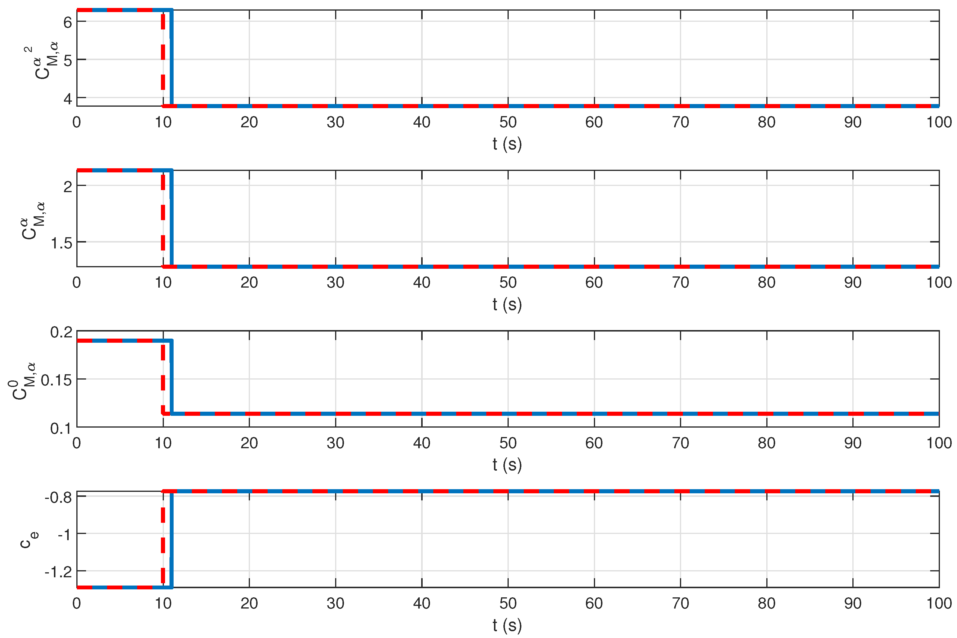
In this section, the proposed HFVDT and the MPSP controller design method is applied to the nonlinear model of HFV, and the details of HFV’s nonlinear mode can be found in [13]. The setting of the simulation is all the same with [13]. For comparison, the fault-tolerant control listed in [34], marked as u F T C , is also adopted and the rate of fault ρ = 0.6 . Then, the proposed MPSP controller is marked as u M P S P , and is applied on HFV. Since HFVDT is constructed online in simulation assuming that the fault occurs at t = 10   s , and the changes in C L , the drag coefficient C D , and moment coefficient C M are listed in Table 1:
From the above table, one can see that when a fault occurs, the aerodynamic coefficient of HFV will all change. But in most literature, only loss of efficiency is considered, just as [34], and δ e r = 0.6 δ e c , where δ e c is the control command and δ e r is the real control input.
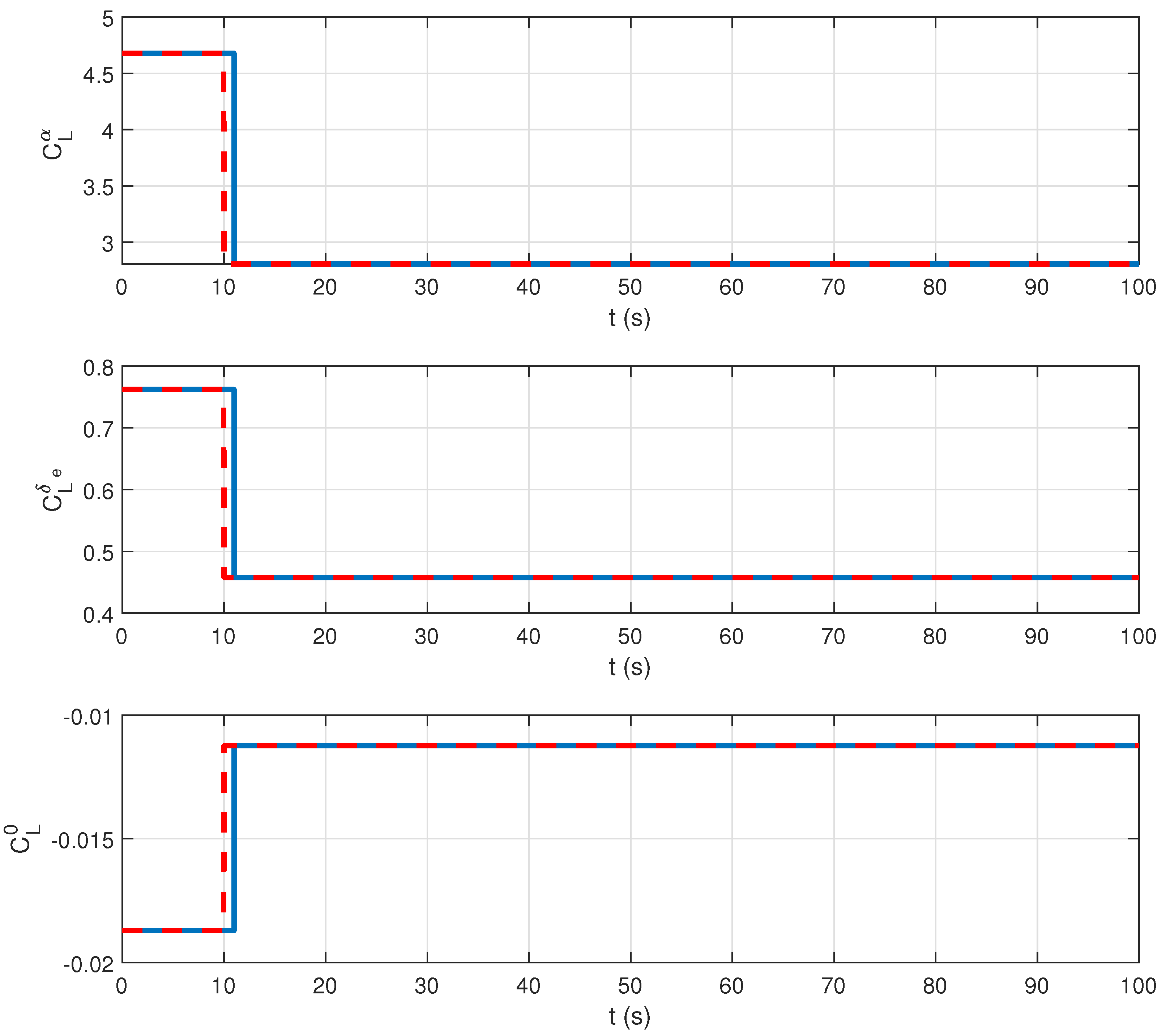
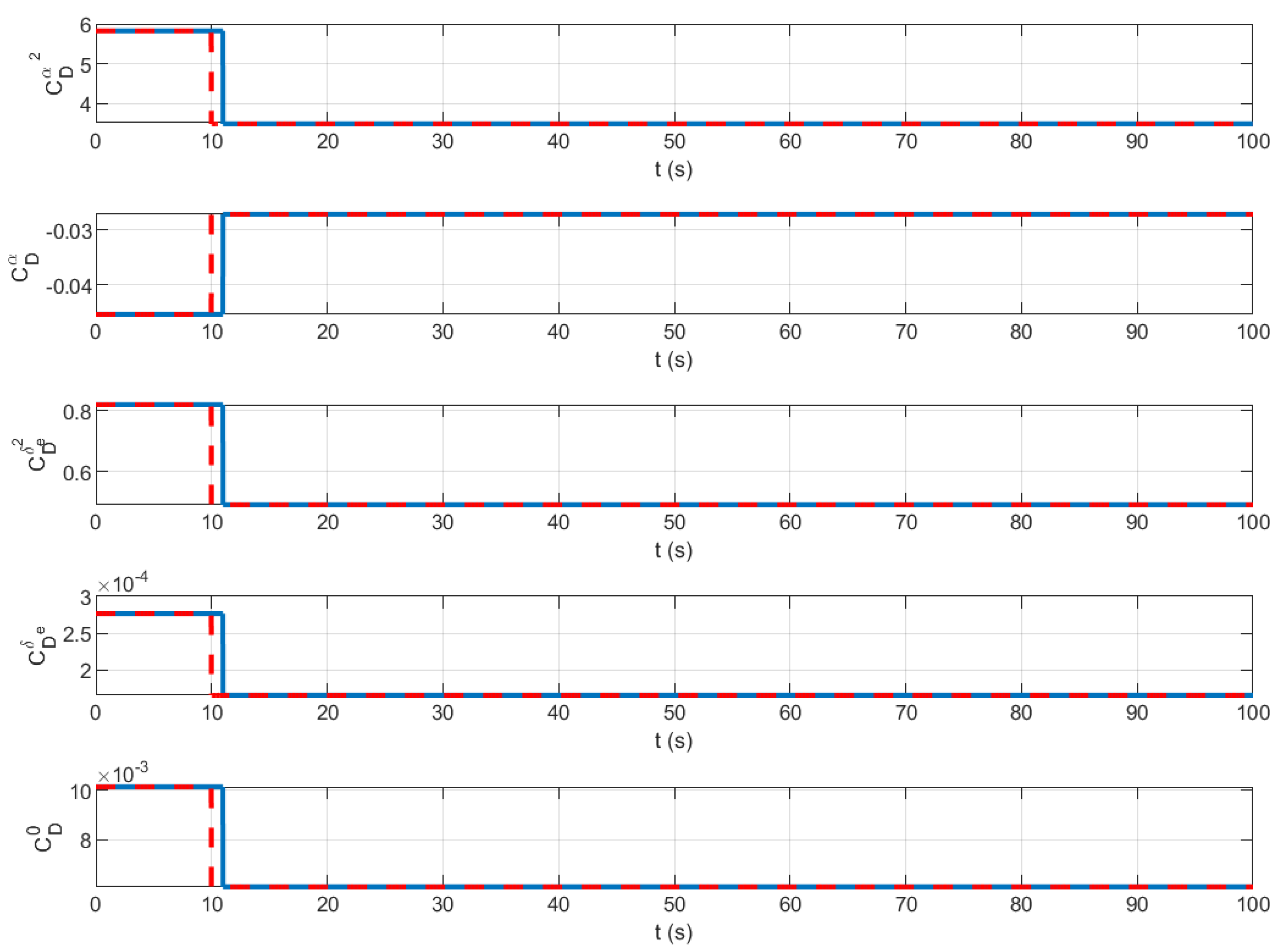
The constructed result of HFVDT is listed in Figure 4, Figure 5 and Figure 6, where the dotted line is the real value of the aerodynamic coefficient of C L , the drag coefficient C D , moment coefficient C M , and the solid line is the online updating result of HFVDT. It is worth noting that with the occurrence of faults, the data of HFV will change, that is, the data of HFV are inconsistent with that without faults. Therefore, it is necessary to set a time window when calculating the aerodynamic coefficient. In this paper, the time window of 1 s is adopted, that is, the data within 1 s before this moment are adopted. From Figure 4, Figure 5 and Figure 6, the online updating result of HFVDT is changed 1 s later than the real value of the aerodynamic coefficient. It can be seen that by setting a time window of 1 s, the aerodynamic coefficient can be calculated in real-time by using the data after the fault.
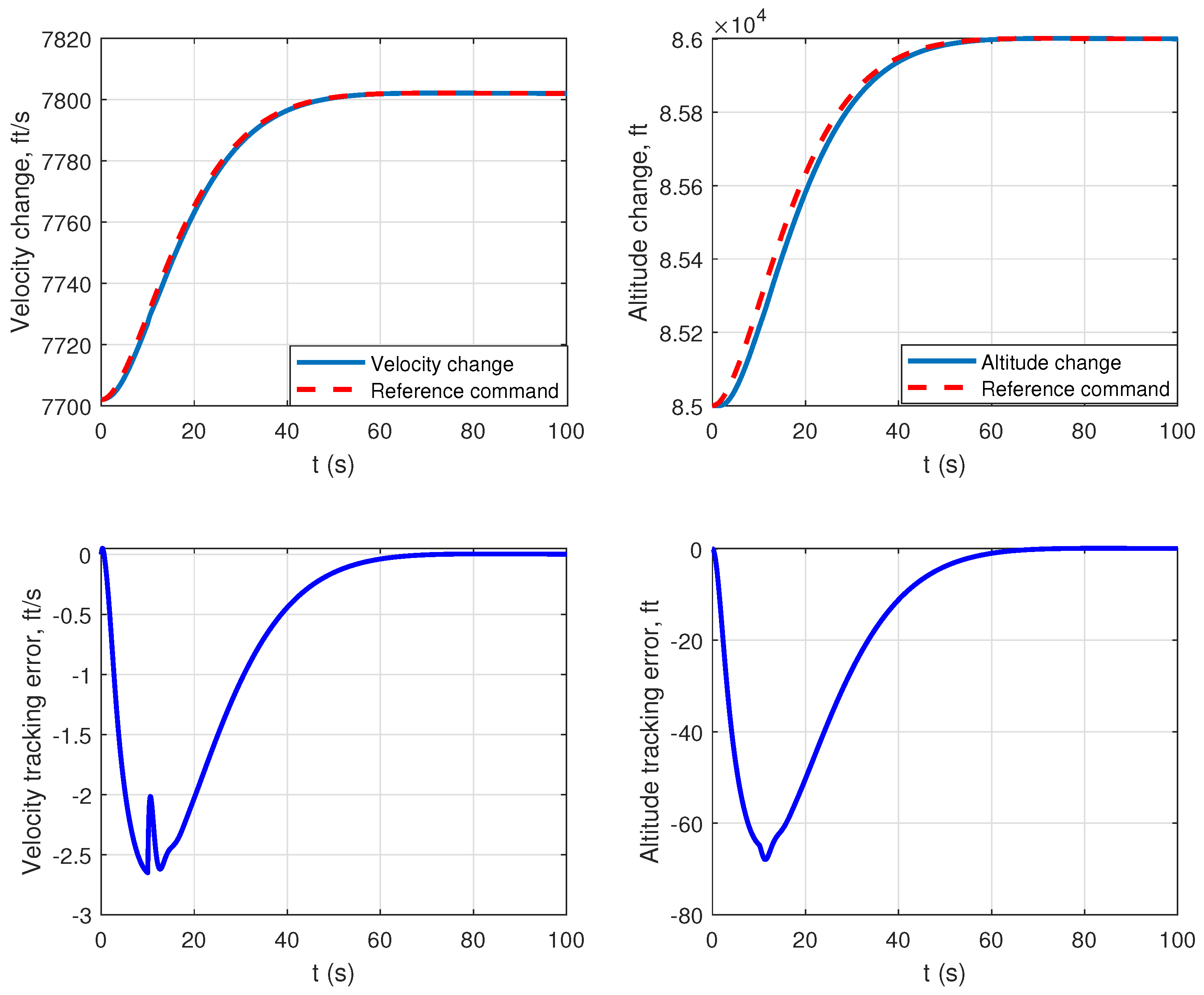
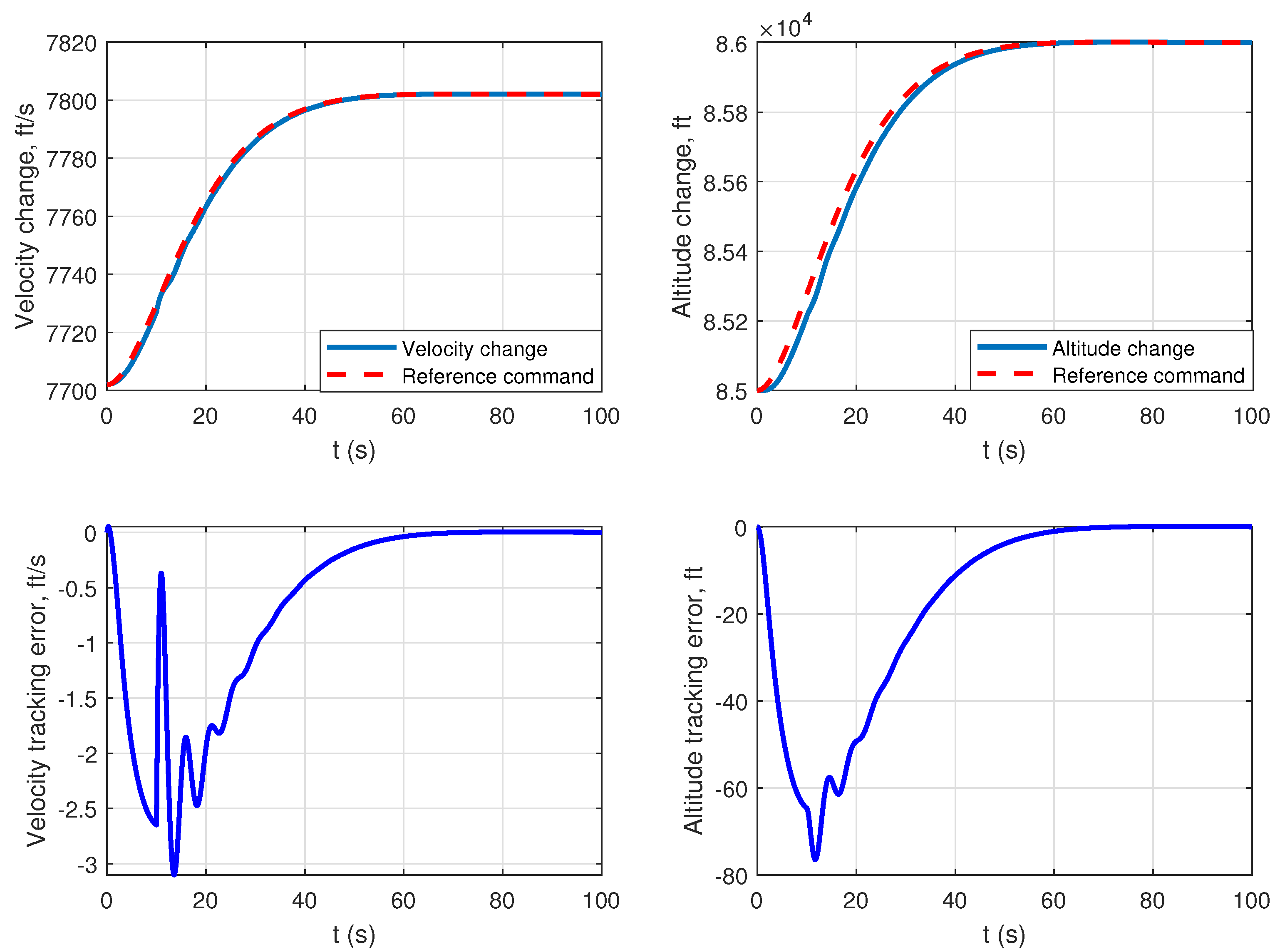
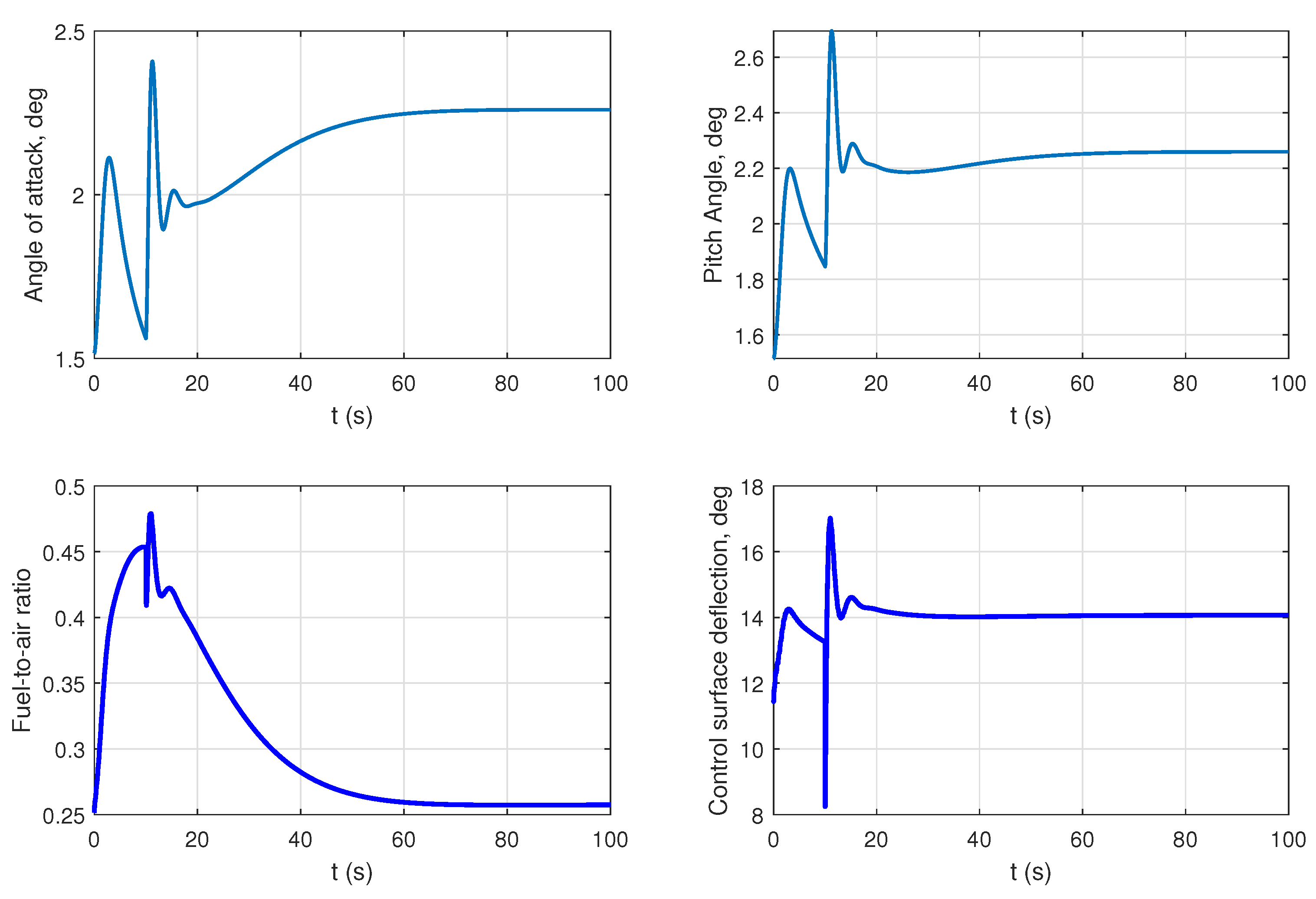
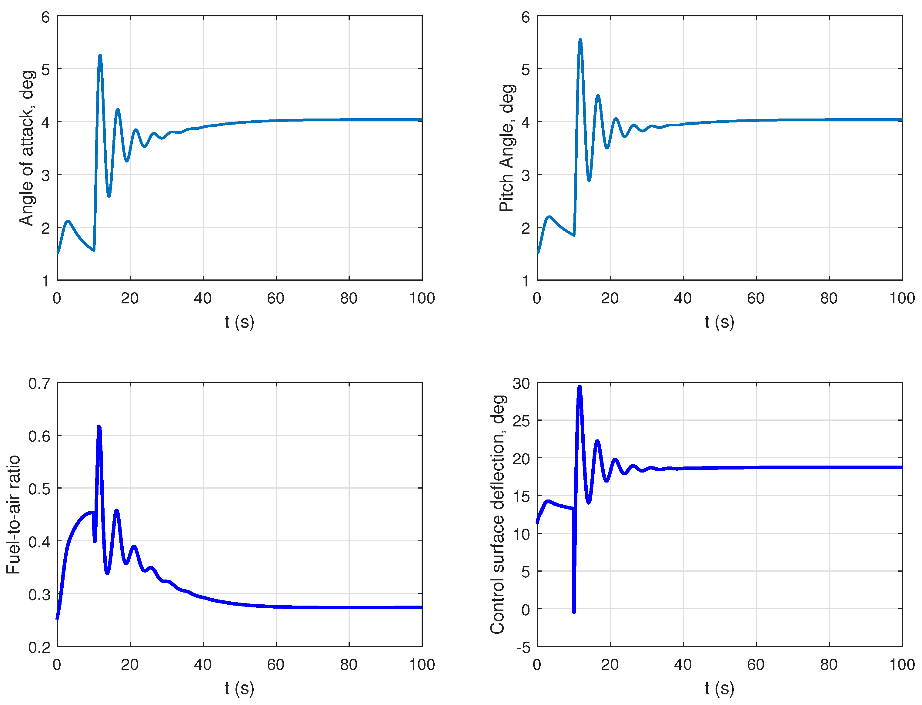
Based on the HFVDT, the proposed MPSP can then be carried out online. The tracking results of u M P S P and u F T C are all listed as follows; the dotted line is the reference command for HFV, and the solid line is the real response of the proposed controller. The tracking results of u M P S P and u F T C are listed in Figure 7 and Figure 8, and the important states together with the input of HFV are given in Figure 9 and Figure 10. The important states of HFV are the angle of attack and flight pitch angle, the input of HFV is fuel-to-air ratio and control surface deflection. From the tracking results of Figure 7 and Figure 8, both u M P S P and u F T C can ensure the accurate tracking of the given command but u M P S P has a smaller tracking error and better tracking effect than u F T C . When fault occurs, u M P S P can quickly achieve stable tracking, while the tracking error of u F T C will fluctuate. This is because u M P S P adopts the DT model, while the design basis of the u F T C controller is still the original nonlinear model. It can be seen that the online DT model of HFV can effectively improve the control accuracy of aircraft.
The important states and input of HFV in Figure 9 and Figure 10 also give the same conclusion. The angle of attack and flight pitch angle of u M P S P are more smooth than those of u F T C . The input of u M P S P is also smoother than that of u F T C . From the above simulation results, it can be seen that the online accurate model of HFV can be obtained by constructing the DT model, and the online accurate control and instruction tracking of HFV can be realized by designing the FTC controller online.

6. Conclusions

In this paper, a DT for HFV is constructed online for controller design, and in the DT, IoT is utilized to collect and transmit information for HFV. The parameter of HFVDT can be updated online according to the change in real HFV. Then an MPSP FTC method is proposed for HFV. Different from the traditional failure hypothesis, when the air rudder is damaged, all associated aerodynamic coefficients of HFV will be changed. In this case, HFVDT is adopted here to reconstruct the nonlinear model of HFV online. Then, the updating law of HFVDT is discussed, and then the MPSP controller design method is utilized. A simulation result on HFV is given to test the effectiveness of the proposed method.
The method proposed in this paper does not consider the measurement error and measurement delay of HFV inertial devices. In fact, due to the complex flight environment of HFV, there are noises, errors and time delays in the measurement results of inertial devices, so it is necessary to eliminate the influence of these factors in practical use. In order to apply the method proposed in this paper in practice, the methods of noise elimination and error compensation in the actual measurement environment still need to be studied, and establishing the DT construction method and controller design method that can be used in the actual environment.

Author Contributions

Conceptualization, D.Z. and S.L.; methodology, X.H.; software, J.X.; validation, D.Z., S.L.; investigation, X.H.; resources, D.Z.; data curation, S.L. and X.H.; writing—original draft preparation, D.Z.; writing—review and editing, S.L. and X.H.; visualization, S.L.; supervision, S.L.; project administration, D.Z.; funding acquisition, X.H. and D.Z. All authors have read and agreed to the published version of the manuscript.

Funding

This work was partially supported by National Natural Science Foundation of China (62073265).

Data Availability Statement

The data presented in this study are available on request from the corresponding author.

DURC Statement

Current research is limited to theoretical research on the control method, which is the beneficial design of a nonlinear system controller and does not pose a threat to public health or national security. The authors acknowledge the dual-use potential of the research involving HFV and confirm that all the necessary precautions have been taken to prevent potential misuse. As an ethical responsibility, authors strictly adhere to relevant national and international laws about DURC. Authors advocate for responsible deployment, ethical considerations, regulatory compliance, and transparent reporting to mitigate misuse risks and foster beneficial outcomes.

Conflicts of Interest

The authors declare no conflict of interest.

Correction Statement

This article has been republished with a minor correction to the DURC Statement. This change does not affect the scientific content of the article.

Nomenclature

The following abbreviations are used in this manuscript:
C D α , δ e drag coefficient
C D α i ith order coefficient of α contribution to C D α , δ e
C D δ e i ith order coefficient of δ e contribution to C D α , δ e
C D 0 constant term in C D α , δ e
C L α , δ e lift coefficient
C L α i ith order coefficient of α contribution to C L α , δ e
C L δ e coefficient of δ e contribution to C L α , δ e
C L 0 constant term in C L α , δ e
C M , Q α , Q contribution to moment due to pitch rate
C M , α α contribution to moment due to angle of attack
C M , δ e δ e , δ c control surface contribution to moment
C M , α α i ith order coefficient of α contribution to C M , α α
C M , α 0 constant term in C M , α α
C T α i Φ ith order coefficient of α in T
c ¯ mean aerodynamic chord
c c canard coefficient in C M , δ e δ e , δ c
c e elevator coefficient in C M , δ e δ e , δ c
Ddrag
gacceleration due to gravity
haltitude
I y y moment of inertia
Llift
L v vehicle length
Mpitching moment
mvehicle mass
N i ith generalized force
N i α j jth order contribution of α to N i
N i 0 constant term in N i
N 2 δ e contribution of δ e to N 2
Qpitch rate
q ¯ dynamic pressure
Sreference area
Ttrust
Vvelocity
xstate of the control-oriented model
α angle of attack
β i h , q ¯ ith thrust fit parameter
γ flight path angle, γ = θ α
δ c canard angular deflection
δ e elevator angular deflection
ξ damping ratio for the Φ dynamics
ξ i damping ratio for elastic mode η i
η i ith generalized elastic coordinate
θ pitch angle
λ i inertial coupling term of ith elastic mode
ρ density of air
Φ stoichiometrically normalized fuel-to-air ratio
ψ ˜ i constrained beam coupling constant for η i
ω natural frequency for the Φ dynamics
ω i natural frequency for elastic mode η i
1 / h s air density decay rate

References

  1. Wu, X.; Xiao, B.; Wu, C.; Guo, Y. Centroidal Voronoi Tessellation and Model Predictive Control-based Macro-Micro Trajectory Optimization of Microsatellite Swarm. Space Sci. Technol. 2022, 2022, 9802195. [Google Scholar] [CrossRef]
  2. Bolender, M.; Doman, D. A nonlinear longitudinal dynamical model of an airbreathing hypersonic vehicle. J. Spacecr. Rocket. 2007, 44, 374–387. [Google Scholar] [CrossRef]
  3. Zhao, D.; Jiang, B.; Yang, H.; Tao, G. Fault-tolerant control of flexible air-breathing hypersonic vehicles in linear ODE-beam systems. Int. J. Control 2020, 93, 820–831. [Google Scholar] [CrossRef]
  4. Bu, X.; Wu, X.; Zhang, R.; Ma, Z.; Huang, J. Tracking differentiator design for the robust backstepping control of a flexible air-breathing hypersonic vehicle. J. Franklin Inst. 2015, 352, 1739–1765. [Google Scholar] [CrossRef]
  5. Zhao, D.; Jiang, B.; Yang, H. Backstepping-based decentralized fault-tolerant control of hypersonic vehicles in PDE-ODE form. IEEE Trans. Autom. Control 2021, 67, 1210–1225. [Google Scholar] [CrossRef]
  6. Xia, R.; Chen, M.; Wu, Q.; Wang, Y. Neural network based integral sliding mode optimal flight control of near space hypersonic vehicle. Neurocomputing 2020, 379, 41–52. [Google Scholar] [CrossRef]
  7. An, H.; Fidan, B.; Wu, Q.; Wang, C.; Cao, X. Sliding mode differentiator based tracking control of uncertain nonlinear systems with application to hypersonic flight. Asian J. Control 2019, 21, 143–155. [Google Scholar] [CrossRef]
  8. Hu, X.; Guo, Y.; Zhang, L.; Alsaedi, A.; Hayat, T.; Ahmad, B. Fuzzy stable inversion-based output tracking for nonlinear non-minimum phase system and application to FAHVs. J. Frankl. Inst. 2015, 352, 5529–5550. [Google Scholar] [CrossRef]
  9. Wu, L.; Yang, X.; Li, F. Nonfragile output tracking control of hypersonic air-breathing vehicles with an LPV model. IEEE/ASME Trans. Mechatron. 2013, 18, 1280–1288. [Google Scholar] [CrossRef]
  10. Ye, H.; Jiang, B. Adaptive switching control for hypersonic vehicle with uncertain control direction. J. Frankl. Inst. 2020, 357, 8851–8869. [Google Scholar] [CrossRef]
  11. Hu, C.; Yang, X.; Wei, X.; Hu, Y. Robust model predictive control for hypersonic vehicle with state-dependent input constraints and parameter uncertainty. Int. J. Robust Nonlinear Control 2021, 31, 9676–9691. [Google Scholar] [CrossRef]
  12. Qi, Q.; Bu, X. Adaptive dynamic programing design for the neural control of hypersonic flight vehicles. J. Frankl. Inst. 2021, 358, 8169–8192. [Google Scholar] [CrossRef]
  13. Hu, X.; Xu, B.; Hu, C. Robust adaptive fuzzy control for HFV with parameter uncertainty and unmodeled dynamics. IEEE Trans. Ind. Electron. 2018, 65, 8851–8860. [Google Scholar] [CrossRef]
  14. Li, W.; Hou, Y.; An, F.; Xia, Q.; Li, Z.; Zhou, Q. Safety Design for the China Space Station. Space Sci. Technol. 2023, 3, 0089. [Google Scholar] [CrossRef]
  15. Chao, D.; Qi, R.; Jiang, B. Adaptive fault-tolerant attitude control for hypersonic reentry vehicle subject to complex uncertainties. J. Frankl. Inst. 2022, 359, 5458–5487. [Google Scholar] [CrossRef]
  16. Armendia, M.; Ghassempouri, M.; Ozturk, E.; Peysson, F. Twin-Control: A Digital Twin Approach to Improve Machine Tools Lifecycle; Springer Nature: Berlin/Heidelberg, Germany, 2019; p. 296. [Google Scholar]
  17. He, R.; Chen, G.; Dong, C.; Sun, S.; Shen, X. Data-driven digital twin technology for optimized control in process systems. ISA Trans. 2019, 95, 221–234. [Google Scholar] [CrossRef]
  18. Meshram, C.; Ibrahim, R.W.; Obaid, A.J.; Meshram, S.G.; Meshram, A.; Abd El-Latif, A.M. Fractional chaotic maps based short signature scheme under human-centered IoT environments. J. Adv. Res. 2021, 32, 139–148. [Google Scholar] [CrossRef] [PubMed]
  19. Vo, D.T.; Nguyen, X.P.; Nguyen, T.D.; Hidayat, R.; Huynh, T.T.; Nguyen, D.T. A review on the internet of thing (IoT) technologies in controlling ocean environment. Energy Sources Part A Recover. Util. Environ. Eff. 2021, 1–19. [Google Scholar] [CrossRef]
  20. Qiu, J.; Tian, Z.; Du, C.; Zuo, Q.; Su, S.; Fang, B. A survey on access control in the age of internet of things. IEEE Internet Things J. 2020, 7, 4682–4696. [Google Scholar] [CrossRef]
  21. Gehrmann, C.; Gunnarsson, M. A digital twin based industrial automation and control system security architecture. IEEE Trans. Ind. Inform. 2019, 16, 669–680. [Google Scholar] [CrossRef]
  22. Wang, J.; Ye, L.; Gao, R.X.; Li, C.; Zhang, L. Digital Twin for rotating machinery fault diagnosis in smart manufacturing. Int. J. Prod. Res. 2019, 57, 3920–3934. [Google Scholar] [CrossRef]
  23. Bujari, A.; Calvio, A.; Foschini, L.; Sabbioni, A.; Corradi, A. A Digital Twin Decision Support System for the Urban Facility Management Process. Sensors 2021, 21, 8460. [Google Scholar] [CrossRef] [PubMed]
  24. Wei, C.; Li, Y.; Yin, Z.; Zhou, L.; Feng, J. On finite-time anti-saturated proximity control with a tumbling non-cooperative space target. Space Sci. Technol. 2023, 3, 0045. [Google Scholar] [CrossRef]
  25. Padhi, R.; Kothari, M. Model Predictive Static Programming: A Computationally Efficient Technique For Suboptimal Control Design. Int. J. Innov. Comput. Inf. Control 2009, 5, 399–411. [Google Scholar]
  26. Maity, A.; Padhi, R.; Mallaram, S.; Rao, G.M.; Manickavasagam, M. A robust and high precision optimal explicit guidance scheme for solid motor propelled launch vehicles with thrust and drag uncertainty. Int. J. Syst. Sci. 2016, 47, 3078–3097. [Google Scholar] [CrossRef]
  27. Kumar, P.; Anoohya, B.B.; Padhi, R. Model Predictive Static Programming for Optimal Command Tracking: A Fast MPC Paradigm. J. Dyn. Syst. Meas. Control 2019, 141, 021014. [Google Scholar] [CrossRef]
  28. Mathavaraj, S.; Padhi, R. Unscented MPSP for Optimal Control of a Class of Uncertain Nonlinear Dynamic Systems. J. Dyn. Syst. Meas. Control 2019, 141, 065001. [Google Scholar] [CrossRef]
  29. Sakode, C.M.; Padhi, R. Computationally Efficient Suboptimal Control design for Impulsive Systems based on Model Predictive Static Programming. IFAC Proc. Vol. 2014, 47, 41–46. [Google Scholar] [CrossRef]
  30. Dwivedi, P.N.; Bhattacharya, A.; Padhi, R. Suboptimal Midcourse Guidance of Interceptors for High-Speed Targets with Alignment Angle Constraint. J. Guid. Control Dyn. 2011, 34, 860–877. [Google Scholar] [CrossRef]
  31. Oza, H.B.; Padhi, R. Impact-angle-constrained suboptimal model predictive static programming guidance of air-to-ground missiles. J. Guid. Control Dyn. 2012, 35, 153–164. [Google Scholar] [CrossRef]
  32. Halbe, O.; Raja, R.G.; Padhi, R. Robust Reentry Guidance of a Reusable Launch Vehicle Using Model Predictive Static Programming. J. Guid. Control Dyn. 2014, 37, 134–148. [Google Scholar] [CrossRef]
  33. Sachan, K.; Padhi, R. Waypoint Constrained Multi-Phase Optimal Guidance of Spacecraft for Soft Lunar Landing. Unmanned Syst. 2019, 7, 83–104. [Google Scholar] [CrossRef]
  34. An, H.; Fidan, B.; Liu, J.; Wang, C.; Wu, L. Adaptive fault-tolerant control of air-breathing hypersonic vehicles robust to input nonlinearities. Int. J. Control 2019, 92, 1044–1060. [Google Scholar] [CrossRef]
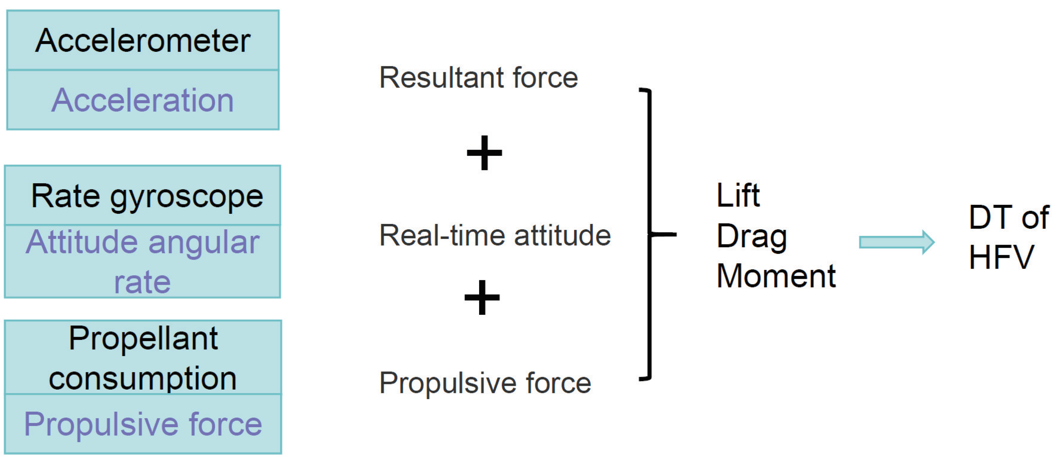
Figure 1. Basic principle of constructing DT.
Drones 08 00460 g001
Figure 2. IoT-based flight data collection and transmission.
Drones 08 00460 g002
Figure 3. Framework of the proposed method.
Drones 08 00460 g003
Figure 4. C L of HFVDT.
Drones 08 00460 g004
Figure 5. C D of HFVDT.
Drones 08 00460 g005
Figure 6. C M of HFVDT.
Drones 08 00460 g006
Figure 7. Tracking result of u M P S P .
Drones 08 00460 g007
Figure 8. Tracking result of u F T C .
Drones 08 00460 g008
Figure 9. Input of u M P S P .
Drones 08 00460 g009
Figure 10. Input of u F T C .
Drones 08 00460 g010
Table 1. Aerodynamic coefficient change caused by the fault.
Before FaultAfter Fault
C L α = 4.6773 C L α = 2.8064
C L δ e = 0.76224 C L δ e = 0.4573
C L 0 = 0.018714 C L 0 = 0.0112
C D α 2 = 5.8224 C D α 2 = 3.4934
C D α = 0.045315 C D α = 0.0272
C D δ e 2 = 0.81993 C D δ e 2 = 0.4920
C D δ e = 0.00027699 C D δ e = 0.0002
C D 0 = 0.010131 C D 0 = 0.0061
C M , α α 2 = 6.2926 C M , α α 2 = 3.7756
C M , α α = 2.1335 C M , α α = 1.2801
C M , α 0 = 0.18979 C M , α 0 = 0.1139
c e = 1.2897 c e = 0.7738
Disclaimer/Publisher’s Note: The statements, opinions and data contained in all publications are solely those of the individual author(s) and contributor(s) and not of MDPI and/or the editor(s). MDPI and/or the editor(s) disclaim responsibility for any injury to people or property resulting from any ideas, methods, instructions or products referred to in the content.