Article

Large-Scale Solar-Powered UAV Attitude Control Using Deep Reinforcement Learning in Hardware-in-Loop Verification

1
National Key Laboratory of Science and Technology on Advanced Light-Duty Gas-Turbine, Institute of Engineering Thermophysics, Chinese Academy of Sciences, Beijing 100190, China
2
School of Aeronautics and Astronautics, University of Chinese Academy of Sciences, Beijing 100049, China
3
Key Laboratory of UAV Emergency Rescue Technology, Ministry of Emergency Management, Beijing 102202, China
4
Beijing Blue Sky Science and Technology Innovation Research Center, Beijing 100190, China
5
Qingdao Institute of Aeronautical Technology, Qingdao 266000, China
*
Authors to whom correspondence should be addressed.
Drones 2024, 8(9), 428; https://doi.org/10.3390/drones8090428
Submission received: 19 June 2024 / Revised: 14 August 2024 / Accepted: 17 August 2024 / Published: 26 August 2024

Abstract

:
Large-scale solar-powered unmanned aerial vehicles possess the capacity to perform long-term missions at different altitudes from near-ground to near-space, and the huge spatial span brings strict disciplines for its attitude control such as aerodynamic nonlinearity and environmental disturbances. The design efficiency and control performance are limited by the gain scheduling of linear methods in a way, which are widely used on such aircraft at present. So far, deep reinforcement learning has been demonstrated to be a promising approach for training attitude controllers for small unmanned aircraft. In this work, a low-level attitude control method based on deep reinforcement learning is proposed for solar-powered unmanned aerial vehicles, which is able to interact with high-fidelity nonlinear systems to discover optimal control laws and can receive and track the target attitude input with an arbitrary high-level control module. Considering the risks of field flight experiments, a hardware-in-loop simulation platform is established that connects the on-board avionics stack with the neural network controller trained in a digital environment. Through flight missions under different altitudes and parameter perturbation, the results show that the controller without re-training has comparable performance with the traditional PID controller, even despite physical delays and mechanical backlash.

1. Introduction

With advances in renewable energy generation, electric systems, and automation control, solar-powered unmanned aerial vehicles (SP-UAV) have experienced increased research interest in the field of aviation due to their characteristics of long endurance and permanent residence. A SP-UAV can continuously provide energy for itself by absorbing solar energy through photovoltaic panels on its body during flight, and execute a long-time mission that cannot be achieved by traditional aircraft. To pursue excellent energy utilization, SP-UAVs often adopt different energy management strategies for lengthening endurance [1,2], such as a method for converting surplus energy into potential energy by climbing and releasing it during the night, which also brings challenges such as the large attenuation of aerodynamic performance with altitude and wind disturbance in different atmosphere conditions for the low-level attitude control capability of a UAV.
Many control methods have been developed in the field of aviation, such as the linear quadratic Gaussian method [3], H-infinite control [4], nonlinear model predictive control [5], etc. However, for solar-powered unmanned aerial vehicles (SP-UAVs), the flight control technology has predominantly continued to rely on traditional Proportional-Integral-Derivative (PID) control and gain scheduling design. For example, the EAV team has implemented a linear PI or PID controller for longitudinal control to bolster stability [6]. The Helios, a distinguished flying-wing SP-UAV, has been designed with autopilot that schedules gains based on airspeed [7]. Additionally, the EL-HASPA aircraft employs a PID-based attitude rate controller that decouples the lateral and longitudinal motions [8]. Despite these efforts, these methods are constrained by their dependence on the known dynamic performance of the aircraft, potentially failing to bridge the gap between the actual system and its linearized model. The gain-scheduling approach, while beneficial, entails repetitive design iterations at various predefined state points, inevitably amplifying the design effort. In stark contrast, learning-based and adaptive intelligent control techniques propose a paradigm shift, offering a more adaptable and comprehensive control framework that could potentially replace the existing controller structures.
Reinforcement learning (RL) constantly pursues the maximum cumulative return through interaction with the real or digital environment to obtain the optimal policy, combining the characteristics of biology, adaptation, and optimization, and shows excellent results in the field of game fighting [9,10], robot arm [11,12], automatic driving [13] and cluster control [14]. For the applications of aircraft control, there is great potential for online reinforcement learning methods that can adaptively update during flight. Van Kampen et al. [15] investigated the practical differences between the proposed Action Dependent Heuristic Dynamic Programming (ADHDP) and Action Independent Heuristic Dynamic Programming (AIHDP) methods in longitudinal motion control of the F-16 model, and the simulation results of online experiments demonstrated the adaptive ability of the controller. Heyer et al. [16] proposed a learning algorithm based on Incremental Dual Heuristic Programming (IDHP) and applied it to the six-DOF nonlinear simulation model of Cessna aircraft, which used a target network to improve the stability of the update. However, online reinforcement learning requires constant exploration during the flight to optimize parameters from never-encountered experiences, just as all reinforcement learning methods need to balance “exploitation” and “exploration”. Determining how to ensure the safety of in-flight controller updating is a complex question, and therefore, all the above works are in the digital simulation stage. Model-free offline reinforcement learning algorithms have shown great application potential in attitude control because they can interact with a digital simulator and be used without re-training in real-world applications which can reduce the damages caused by online exploration. Pi et al. [17] applied the improved deterministic policy algorithm to train the quadrotor controller and then deployed the neural network to the flight platform to test its stability in the real environment. Wada et al. [18] employed deep reinforcement learning Asynchronous Advantage Actor-critic (A3C) algorithm to the wind tunnel test of pitch control and they investigated the influence of physical friction and delay on the real control performance. Kaufmann et al. [19] developed the SWIFT system and deployed it in FPV drones. The system combines deep reinforcement learning (RL) in a simulated environment with data collected in the physical world. SWIFT won several races against each of the human champions and demonstrated the fastest recorded race time. Based on the above experiments, the neural network controller was directly transferred to the small aircraft platform after training and conducting a flight test to verify its performance difference in the established digital environment and the real world, which is called the “reality gap” in RL problem [10]; however, the SP-UAV has a higher cost and larger size compared with the above-mentioned research objects, so more secure verification methods are needed. Compared with the real flight and pure digital simulation, the hardware-in-loop (HIL) real-time simulation experiment implemented on the ground has lower cost and risk by incorporating real cables, sensors, and servos into the platform, which can simulate real application scenarios to a certain extent and improve the efficiency of control design [20,21].
The contribution of this work is twofold:
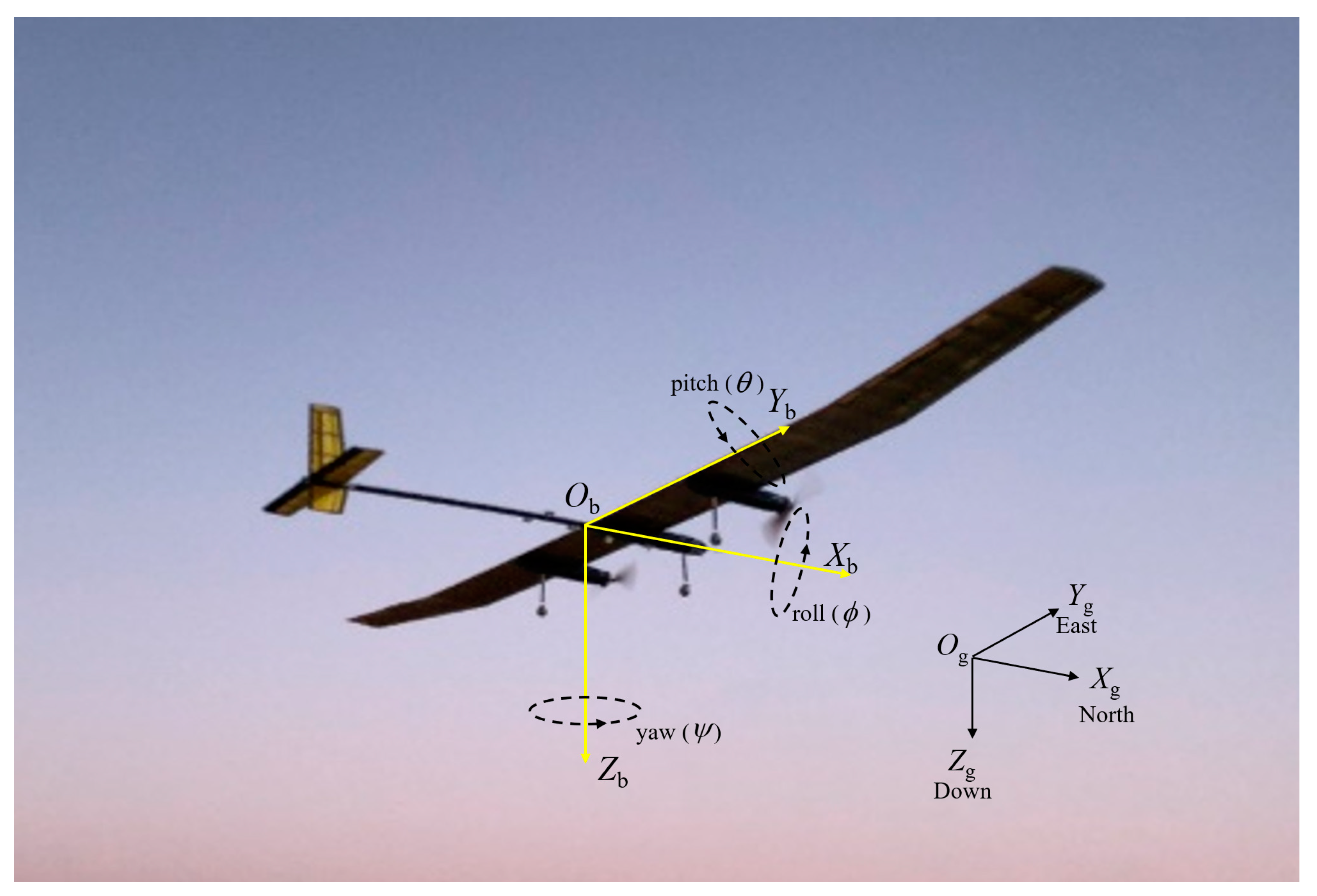
  • In this work, the self-designed and developed high-altitude long-endurance SP-UAV is taken as the research object, as shown in Figure 1, and a neural network controller is designed to meet requirements of tracking the specified attitude based on the deep reinforcement learning (DRL) framework.
  • A hardware-in-loop simulation platform is established which can verify the effectiveness of the trained neural network controller with different flight tasks. And the simulation platform has the characteristics of strong generality that can be quickly modified and used in other aircraft configuration or algorithm testing.
The rest of this work is organized as follows: Section 2 describes the dynamics model, kinematic model, and other necessary parts for the simulation environment. Section 3 introduces the RL framework used to design the controller and represents the specific settings in detail. In Section 4, the built hardware-in-loop simulation platform is introduced. Section 5 presents the main experimental results obtained in the digital simulation and HIL simulation. Finally, Section 6 summarizes the views on the presented work and ideas for future research.

2. Mathematical Model

2.1. Dynamics and Kinematics Model

The rigid body is used to model the UAV for simulation. The complete state space can be obtained by adopting the Runge–Kutta method to solve the six-DOF dynamics and kinematics equations in the form of ODE.
In the simulation process, assuming that the body’s translational motion is represented by V b = [ u , V , w ] T , and the rotational angular velocity is represented by ω = [ p , q , r ] T , the flight motion equations can be described as Equation (1):
m ( V ˙ b + ω × V b ) = F x F y F z = F I ω ˙ + ω × I ω = M x M y M z = M
where m is the aircraft mass, I is the inertia tensor, [ F x , F y , F z ] T and [ M x , M y , M z ] T , respectively, represent the components of the resultant force and torque on the three axes of the aircraft in the nose-right-down body coordinate system that is rigidly attached to center of mass. The force and torque during flight can be divided into three categories according to the source: gravity, aerodynamic force, and force generated by propeller thrust, as seen in Equations (2)–(5).
F = F gravity + F aero + F prop
F gravity = R g b 0 0 m g , F aero = R w b 1 2 ρ V a 2 S C D 1 2 ρ V a 2 S C Y 1 2 ρ V a 2 S C L , F prop = T x T y T z
M = M aero + M prop
M aero = 1 2 ρ V a 2 S b C l c C m b C n , M prop = l prop m prop n prop
where g and ρ are the local gravitational acceleration and air density, Va is the airspeed, S is the wing area, b is the wing span, and c is the wing chord. R g b , R w b in Equation (3) represent the transformation matrices from earth-fixed frame to body-fixed frame and from aerodynamic coordinate system to body-fixed frame, respectively, as shown in Equations (6) and (7):
R g b = c θ c ψ c θ s ψ s θ s θ s ϕ c ψ c ϕ s ψ s θ s ϕ s ψ + c ϕ c ψ s ϕ c θ s θ c ϕ c ψ + s ϕ s ψ s θ c ϕ s ψ s ϕ c ψ c ϕ c θ
R w b = c β c α s β c α s α s β c β 0 c β s α s β s α c α
where α is attack angle and β is sideslip angle.
For aerodynamic coefficients, the term C L is total lift coefficient, C D is total drag coefficient, C Y is total normal force coefficient, C l is total rolling moment coefficient, C m is total pitching moment coefficient, and C n is total yawing moment coefficient. Their specific components are as follows:
C L = C L 0 + C L α α + C L β β + C L q q + i C L δ i δ i + C L x ˙ x ˙ C D = C D 0 + C D α α + C D β β + i C D δ i δ i + C D x ˙ x ˙ C Y = C D 0 + C Y β β + C Y p p + i C Y δ i δ i + C Y x ˙ x ˙ C l = C l 0 + C l β β + C l p p + C l r r + i C l δ i δ i + C l x ˙ x ˙ C m = C m 0 + C m α α + C m β β + C m q q + i C m δ i δ i + C m x ˙ x ˙ C n = C n 0 + C n β β + C n p p + C n q q + C n r r + i C n δ i δ i + C n x ˙ x ˙
In the expression of lift coefficient C L , C L 0 is the basic part, C L α α is the increment of lift coefficient with attack angle, C L β β is the increment of lift coefficient with sideslip angle, C L q q is the increment of lift coefficient with rate, C L δ i δ i is the increment of lift coefficient with control surfaces, and C L x ˙ x ˙ is the increment of lift coefficient with fuselage elastic deformation. The terms in the expression of other coefficients have similar meanings and their notation is adapted from Beard’s book [22]. In the design stage, aerodynamic coefficients at different state points depending on the Mach number, attack angle or control surfaces were obtained by computational fluid dynamics method. Aerodynamic parameters at any time can be solved by linear interpolation method and part of the data are available in [21]. For the force and torque created by the propeller thrust, they are measured and recorded through the experiment under different height, flow speed and throttle in wind tunnel.
The formula between [ p , q , r ] T and the rate of Euler angle can be determined by Equation (9), and the conversion between inertial frame velocity and body velocity is shown in Equation (10).
Θ ˙ = ϕ ˙ θ ˙ ψ ˙ = 1 sin ϕ tan θ cos ϕ tan θ 0 cos ϕ sin ϕ 0 sin ϕ sec θ cos ϕ sec θ p q r
x ˙ = x ˙ y ˙ z ˙ = ( R g b ) T u V w
where ϕ , θ , ψ are roll angle, pitch angle and yaw angle, respectively. x , y , z are the position of the aircraft in inertial coordinates that is north-east-down (NED) frame that is rigidly attached to the take-off point. Basic parameters of the studied aircraft are displayed in Table 1.

2.2. Environmental Model

There is a big span of flight altitudes for the studied SP-UAV in this work, which causes the differences in air density around the body. The 1976 American Standard Atmospheric model [23] is employed to obtain the atmospheric information of the aircraft position in the control simulation process. And the gravitational acceleration is obtained according to the developed WGS 84 model.
Turbulent wind is a continuous random fluctuation superimposed based on constant wind, which is equivalent to a random quantity fluctuating around an average value. The Dryden Wind Turbulence Model was established in the present work by referring to MATLAB/Simulink [24] and Bohn et al.’s work [25] to generate random wind fields at different heights.

2.3. Actuator Model

The first-order inertia model is developed to simulate the dynamic performance of the real servo and prepare for the subsequent reinforcement learning training environment. The transfer function of each actuator can be expressed as follows:
δ i ( s ) δ i c ( s ) = 1 T s + 1
where δ i , i a , e , r , t represents the deflection angle of aileron, elevator, rudder, and the throttle of propeller speed, while the superscript c denotes the corresponding control command. For each control surface, the time constant T is set to 0.02 s and the deflection rate is limited to 100°/s, while for the propulsion system, the time constant T is set to 0.2 s, and the rate of change is limited to 480 rpm/s. Here, elevator δ e is defined to be positive for downward deflection, rudder δ r is defined to be positive for left deflection when looked forward from the tail, and for aileron δ a , right aileron is defined to be positive for downward deflection and left aileron is positive for upward deflection.
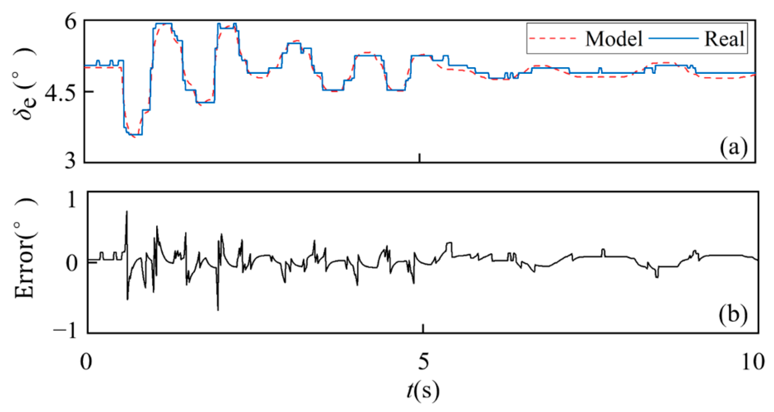
To compare the similarity between the simulation and the real servo, the same command is sent to the mathematical model and the real servo without load. Then feedback values of above two are recorded and the curves are shown in Figure 2. It can be seen from Figure 2a that the dynamic response trends of the real hardware and the mathematical model are in good agreement. Due to the introduction of analog quantity and the setting of data transmission accuracy, the real servo feedback still has a step-like “burr” phenomenon under the stable level. In order to quantitatively describe the gap, the response output values of the two at the same time are subtracted to obtain Figure 2b, which shows that the absolute error is within 1° and mainly occurs when the instructions change rapidly.

3. Low-Level Controller Based on Reinforcement Learning

The aircraft is capable of executing designated flight missions through a conventional control system depicted in Figure 3. This system comprises a task planning or logical processing module that, after signal processing, generates specific states. Subsequently, a high-level control module formulates attitude and speed directives based on the flight path or target data. These directives are then precisely followed by a low-level controller, which manipulates the control surfaces and throttle directly.
Our approach introduces a novel element: the application of a deep reinforcement learning algorithm to develop an inner-loop neural network (NN) controller for solar-powered aircraft, as shown in Figure 1. This NN controller is designed to produce actuator commands directly from the current vehicle attitude, thereby efficiently tracking the attitude and speed commands issued by any outer-loop control module, such as those responsible for navigation or guidance.
Furthermore, this controller is not only innovative in its design but also in its application. It meets the criteria for hardware-in-loop simulations, providing a robust platform for real-world implementation verification.

3.1. Reinforcement Learning Framework

The reinforcement learning problem can be defined as a Markov Decision Process (MDP) where the controller observes the state of the external environment and selects the action according to a policy π . The MDP process can be defined through the four-tuple group ( S , A , R , P ) , where the state s S , action a A , S and A denote the state space and action space, respectively. The state transition probability P represents the probability from s t to s t + 1 when the action a t is taken at time t . At the same time, the environment generates an immediate reward r t = R ( s t , a t ) . The optimal strategy π * is expressed as one that can obtain the maximum expected total reward, which is defined as:
π * = argmax π E a t ~ π ( | s t ) t γ t r t
The Soft Actor-Critic (SAC) algorithm [27] is adopted to carry out the following work, which is an off-policy and off-line reinforcement learning framework based on entropy maximization. At each state transition, the controller receives a reward related to the entropy of the policy. Compared with other reinforcement learning algorithms, it can improve the exploration efficiency, and the algorithm suitable for continuous space is less sensitive to hyperparameters. The process of finding the optimal policy in the SAC algorithm can be rewritten as follows:
π * = argmax π E a t ~ π ( | s t ) t γ t ( r t + η H ( π ( | s t ) ) )
where the entropy H ( π ( | s t ) ) = E π log π ( | s t ) and it is traded-off against future rewards with the temperature parameter η .
The policy in the present work is modeled as a multivariate Gaussian distribution to construct the action: the mean μ θ and covariance σ θ are output through a neural network (NN) with parameters θ . The Q-function critic is parameterized as another neural network with parameters ϕ and it can be obtained in a recursive form in Equation (14) by using the Berman equation when entropy is introduced:
Q ϕ ( s t , a t ) = E a t , a t + 1 ~ π θ r t + γ ( Q ( s t + 1 , a t + 1 ) η log ( π θ ( a t + 1 | s t + 1 ) )
The SAC algorithm uses double Q-function trick by learning two neural networks Q ϕ 1 , Q ϕ 2 and pessimistic strategy to reduce the overestimation bias. For stability of learning, the target Q-function networks with parameters ϕ 1 , ϕ 2 are introduced to make the gradient update follow a more constant direction and soft updates are periodically made by smoothing factor τ between ϕ i and ϕ   i . As an off-policy method, the SAC algorithm can improve data utilization efficiency by storing experience in replay buffer D . The mean squared Bellman error for the Q-function loss can be expressed in Equation (15):
J Q ( ϕ   i ) = E ( s t , a t , r t , s t + 1 ) ~ D a t + 1 ~ π θ 1 2 Q ϕ i ( s t , a t ) r t + γ ( min i = 1 , 2 Q ϕ i , ( s t + 1 , a t + 1 ) η log π θ ( a t + 1 | s t + 1 ) ) 2
Unlike the deterministic strategy, the stochastic policy means that the objective in Equation (13) depends on the expectation over actions and it is therefore non-differentiable. So, in the SAC algorithm, a reparameterization trick is proposed to use the mean and standard deviation of the policy network output along with independent noise ζ , as shown in Equation (16), where E is the identity matrix.
a ˜ t = tanh ( μ θ ( s t ) + σ θ ( s t ) ζ ) , ζ ~ N ( 0 , E )
Finally, the loss function of policy is deduced in Equation (17)
J π ( θ ) = E ( s t , a t , r t , s t + 1 ) ~ D min i = 1 , 2 Q ϕ   i ( s t , a ˜ t ) η log π θ ( a ˜ t | s t )

3.2. Controller Design

In the designed framework, the controller will receive the current flight information and feed it to the policy neural network to provide the action for the control surfaces and throttle. Referring to previous studies [25,27] where the researchers took full state variables in dynamics and kinematics models as current information, the specific state s t at each timestep in the present work is empirically designed as:
s t = z , ϕ , θ , p , q , r , V eas , α , β , δ a , δ e , δ r , δ t | | g t T
where the flight altitude z is explicitly added to the state and the yaw angle ψ is discarded because the performance is greatly affected by the large-span altitude and the direction of the vehicle is mainly controlled by roll angel given by path tracker in outer-loop controller. The current actuator status is also transmitted to the controller and it is expected to automatically process the feedback information. Compared with the full flight information, the lower dimension of the above representation is conducive to the convergence process of reinforcement learning. The target attitude g t can be represented independently and be dynamically changed using any way in the simulation:
g t = ϕ cmd , θ cmd , V eas , cmd T
It is worth mentioning that the equivalent airspeed Veas is used to characterize the speed in view of the change in flight altitude and air density will lead to a large range of true airspeed Va, which the two airspeed values can be converted by the local density ρ and the standard atmospheric density at sea level ρ 0 through the following equation:
V eas = ρ 0 ρ × V a
According to vehicle configuration, the action vector under direct control can be written as
a t = [ δ a c , δ e c , δ r c , δ t c ] T
and the meaning of the symbols are referred to in Section 2.3.
All of the attitude and action commands are physically constrained and their ranges are shown in the following Table 2.
One of the most critical design factors in goal-oriented reinforcement learning controllers is the reward function. In this work, the reward r t consists of one positive parameter called survival reward and four negative cost terms, as shown in Equation (22). The survival reward, here a constant value 1, is taken to ensure the reward is always positive and avoid the “suicide” behavior of the aircraft that will obtain the maximum cumulative reward in the early learning process. In order to accurately track the reference values, the cost terms p ϕ , p θ , p V eas , p β are set in the forms related to the absolute value of the error and are limited by bounds. The sideslip angle is also taken as one factor of the penalty terms to avoid the aerodynamic performance deterioration. In Equation (22), the numbers 5, 6, and 30 in the denominator are all for the purpose of normalization. The 0.3 is an adjustable value. The goal is to keep the error within a smaller range to ensure safe control accuracy. These parameters will affect the control effect of the controller. When the error limit is reduced, the training time will be extended to some extent.
r t = 1 p ϕ p θ p V eas p β p ϕ = min ( ϕ t ϕ cmd 5 , 0.3 ) p θ = min ( θ t θ cmd 6 , 0.3 ) p V eas = min ( V eas , t V eas , cmd 5 , 0.3 ) p β = min ( β t 30 , 0.1 )

3.3. Architecture Design

The architecture of the neural network policy, i.e., the attitude controller for the following verification experiment constructed in this study is shown in Figure 4. Since the input of the controller does not contain all the information, and it is impossible to accurately model the disturbance in the real world, the controller is expected to have the ability to process the past dynamic information, just like the differentiation and integration in the PID control methods. A Long-Short Term Memory (LSTM) network [28] is a very suitable choice [12]. Therefore, after extracting the dynamic information by a single-layer LSTM network with 64 hidden state dimensions, the output is projected to the action dimension using two fully-connected (FC) layers, where each layer has 256 neurons accompanied by a ReLU activation function. The Gaussian policies with mean μ and covariance σ are output actions through which Tanh activation is clipped to lie within the control range. However, in the evaluation phase we force σ = 0 to obtain the more stable outputs. Considering the influence of the introduction of LSTM on the stability of the training process, that is, when the off-policy algorithm uses the historical data, the network parameters may be unable to adapt to the cell state output by LSTM at that time, so we directly input the states of the eight historical steps into LSTM layer, and store them as whole into the experience buffer for later training. The architecture of a Q-function network is like that of an action network, except that the extracted dynamic information after LSTM is directly stacked with actions through the fully connected layer, and only the unique value of the current state–action pair is output at last.

3.4. Training Setting

Under training process conditions, all models introduced in Section 2 are realized in C++ code and solved ODE equations are based on the four-order Runge–Kutta method by Boost package. The model data interact with the SAC algorithm and the neural network developed with the PyTorch framework through the Pybind package. The hyperparameters of the SAC algorithm are consistent with those of Haarnoja et al. [27].
Both the policy and Q-function model are trained with a learning rate of 3 × 10⁻⁴ using the ADAM optimizer [29]. In total, 256 samples are randomly drawn from the replay buffer for training each time. The number of hidden layers is 2. The number of hidden units per layer is 256. The temperature coefficient α is fixed at 0.2, and the reward discount coefficient γ is set at 0.99. The capacity of the replay buffer is set to be 1 million. The smoothness factor in the target network update operation is set to 0.005. The target update interval is 1, and gradient steps is 1. In order to ensure the action output is smoother, the CAPS algorithm [30] is adopted whose regularization weights κS and κT are 2 and 1, respectively.
The controller observes the current state where every 40 ms–60 ms an interval is randomly assigned and fixed at the start of the episode. Each episode has a maximum of 500 interactions. Considering the real signal lag and actuator delay, 80 ms–120 ms delay is added in the training process according to the control cycle of each episode. It is believed that this delay is a serious overestimation for the test system in the real world, but it has been proved by previous studies that the controller trained under high delay can be downward compatible with low delay [18]. Due to the measurement error of the real device, sensor noise is superimposed on the raw state in the form of an OU process [31] and then the state will be fed into the neural network during training. The OU process can generate time-related sequence noise that is more suitable for the inertial system compared with the Gaussian noise. Therefore, the observed state s ^ t at each moment is:
s ^ t = s t + n t , n t O U μ m , σ m , θ m
where s t is the raw state obtained by mathematical model calculation without noise, n t is the measurement noise which is generated based on OU process with the mean μ m = 0 , the mean regression rate θ m = 0 , and the different variance σ m shown in Table 3.
As an important method to improve the robustness of the deep reinforcement learning controller and narrow the gap between simulation and reality, the domain randomization technique is used in the training process. The model parameters are randomly selected and sampled by uniform distribution U ( low ,   high ) at the start of each episode according to the ranges shown in Table 4. The turbulent wind was also applied to the aircraft during the training. Considering the aircraft’s own tolerance, the absolute values of wind speed components in three directions were limited to 2 m/s and the absolute values of angular velocity caused by turbulence were limited to 0.3°/s.

4. Hardware-in-Loop Simulation Platform

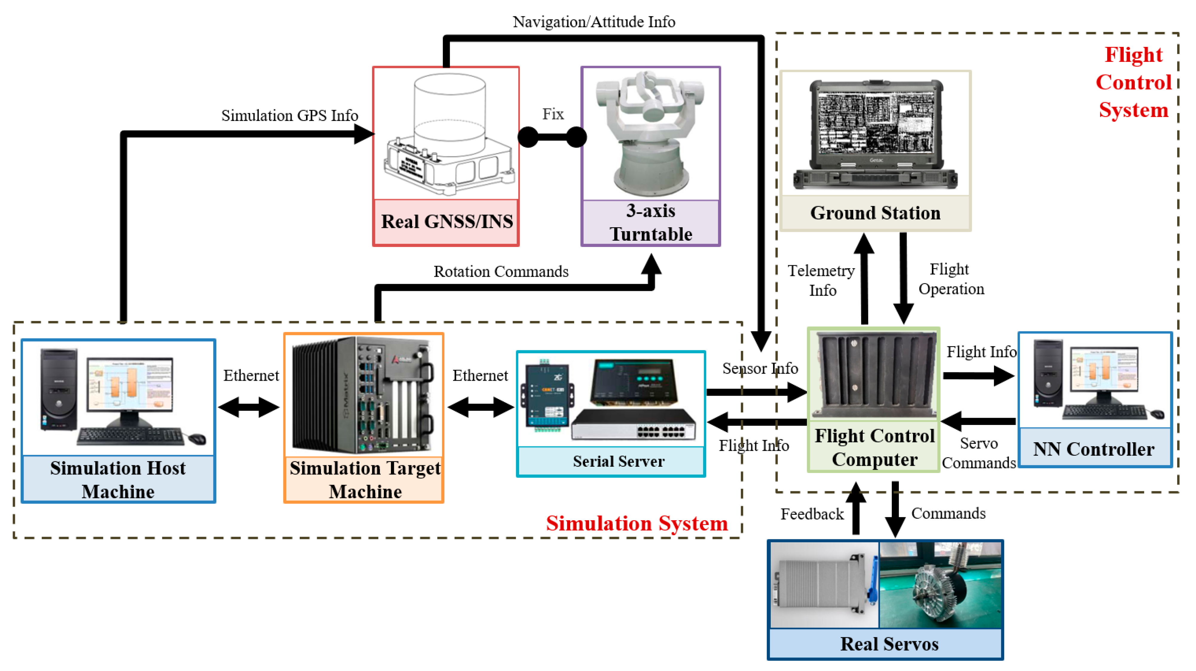
An open-source autonomous driving suite may not satisfy the reliability requirements in harsh near-space environments for SP-UAVs, so the aircraft needs to equip particular sensors and avionics devices, which also imposes demands for adaptability on the hardware testing platform. To this end, the customized hardware-in-loop simulation platform used in this work is shown in Figure 5, which can be divided into three parts: the UAV real-time simulation system based on xPC Target, one flight control computer running the complete autopilot program, and the custom avionics stack. This part is only used for the validation of the controller and does not participate in any neural network training process.

4.1. UAV Simulation System Based on xPC Target

The real flight is not the preferred verification method in the design stage, but the real-time simulation system can take advantage of mathematical models to reflect the aircraft performance benefited by fast development. The UAV real simulation system in this platform consists of two parts: (1) The host machine that uses the Real-Time Workshop (RTW) tool to generate code for the simulation model and load it into the target machine. At the same time, it can communicate with the lower computer through an ethernet connection for communication to realize the control and monitoring of the simulation process of the lower computer. (2) The target machine running the generated code to solve the equations of UAV dynamics and kinetics models, actuator models and sensor models described in Section 2 during the simulation. All models are run at a fixed frequency of 100 HZ using the four-order Runge–Kutta method and built in MATLAB/Simulink. The simulation system and the flight control computer communicate with each other according to the actual interface protocol between the actuator and the sensor through I/O interfaces.
In addition, the system also includes the serial port server and switch for the conversion and exchange of different signal forms.

4.2. Real Flight Control and Management System

The flight control and management system consists of three parts: flight control computer, ground control station and neural network module.
The flight control computer runs the real-time operating system and the customized autopilot program, which can receive and parse sensor signals through different I/O interfaces, including radio altimeter (LRRA), barometer, and Global Navigation Satellite System/Inertial Navigation System (GNSS/INS) information. According to the requirement, the autopilot in the flight control computer can achieve flight decision, trajectory tracking, attitude control as well as responding to the instruction sent by the ground staff. In addition, it is responsible for sending the command and reading the feedback of all kinds of actuators. As a console, the ground control station receives and displays the flight attitude information and hardware status forwarded by the flight control computer in the form of a graphical interface. At the same time, it can make decisions and control the flight process by sending different kinds of instructions to the flight control computer. In the real flight test, the above two realize the information interaction between heaven and earth through the wireless transmission link equipped by the aircraft. In order to simplify the experiment, in the hardware-in-loop simulation process, the ground control station is simulated to conduct a wired cross-link with the flight control computer through the serial port signal.
The trained neural network module is deployed on the laptop and implemented with Python code. The flight state obtained by the flight control computer is sent to the neural network controller in the form of an RS422 serial signal, and the neural network calculates the actuator command immediately by forward inference which will be sent to the actuators through the serial signal after the corresponding operation in the flight control computer. This timing task is triggered by the flight control computer’s internal clock.

4.3. Real Custom Avionics Stack

The real GNSS/INS system is fixed on the three-axis servo turntable platform and rotates synchronously with the turntable plane; the specific parameters and indicators are shown in Table 5 and Table 6. During the experiment, the simulation target computer will calculate the current attitude and angular velocity of the aircraft, and this information is transmitted by fiber channel (FC) connections to a three-axis turntable. While fixed on the rotating platform, the inertial navigation system is able to measure the current installation plane’s corresponding angle information (roll angle, pitching angle, yaw angle, and the corresponding angular velocity) which are fed back to the flight control computer through serial signals to realize the simulation of the aircraft’s flight attitude. At the same time, the GPS and linear velocity obtained by the simulation target computer are also transmitted to the GNSS system directly to form position information.
The real actuator system includes the servos and direct drive motor. In this work, six servos of the VOLZ DA30 series are incorporated into the hardware-in-loop simulation system according to the layout of the aircraft, as the driving mechanism of the left aileron, right aileron, rudder, steering wheel, left elevator, and right elevator. The deflection command is transmitted by the flight control computer, and its current angle feedback is collected in real-time. In this experiment, the real motor and propeller are not connected, but the mathematical model is used for simulation. The operating data and performance of the used servo are shown in Table 7.
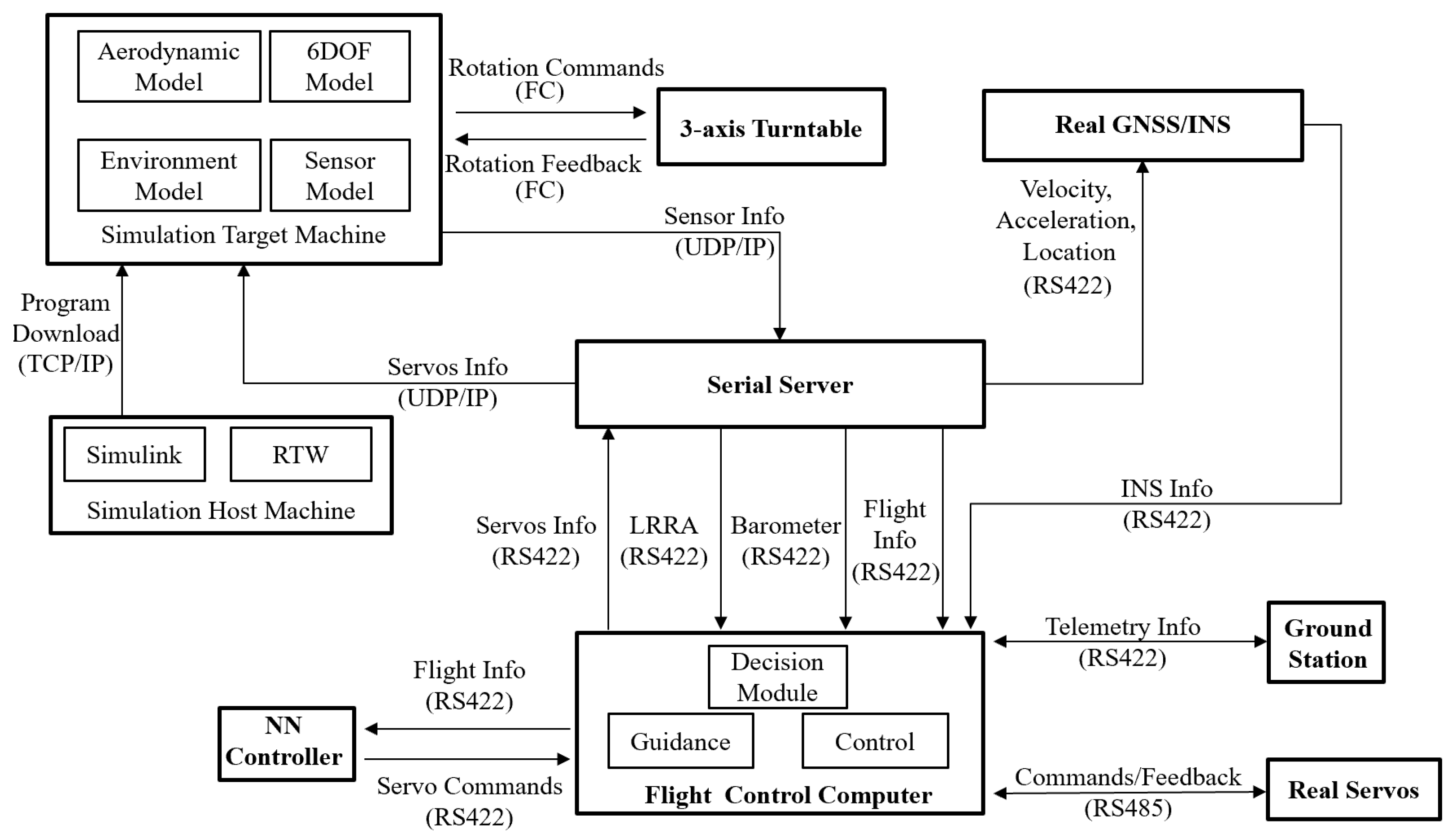
Based on the above introduction, the signal pathway of the hardware-in-loop real-time simulation test platform for neural network attitude control is shown in Figure 6, where the abbreviations in parentheses are different communication forms. All real avionics are connected and communicated with the flight control computer via onboard power or signal cables. Figure 7 shows the whole picture of the simulation platform from different angles.

5. Results and Discussion

5.1. Training Performance in Digital Environment

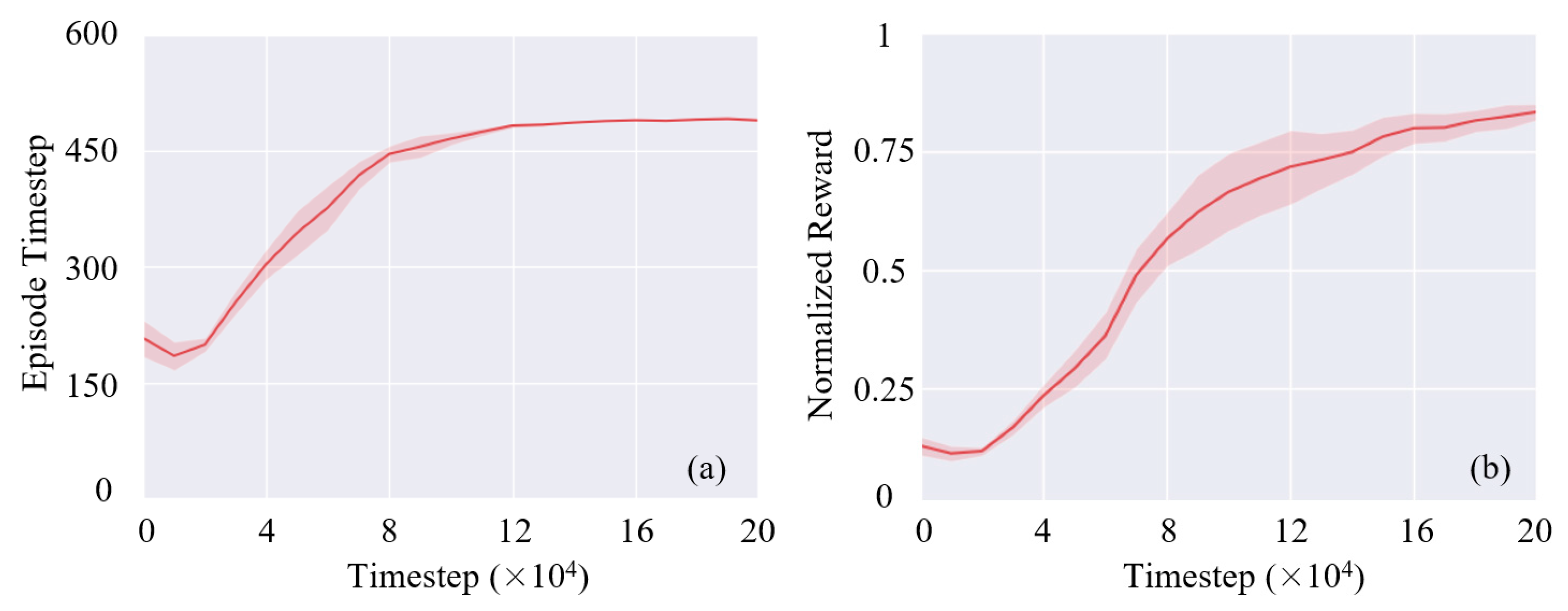
The training progress under five different random number seeds is shown in Figure 8, where the reward is normalized by dividing the maximum episode reward by 500. It is inspiring that the neural network only needs 0.2 million timesteps to converge, which takes an average of only 1 h and 20 min on a workstation with a GTX 2080TI GPU and Intel Xeon Gold 6142 CPU. Compared with the traditional design mode of researchers, the application of neural networks for controller design will greatly reduce the research time. The trained policy network can be deployed without any compression on a laptop computer with an i5-10210U CPU, with an average cost of about 1 ms per inference.
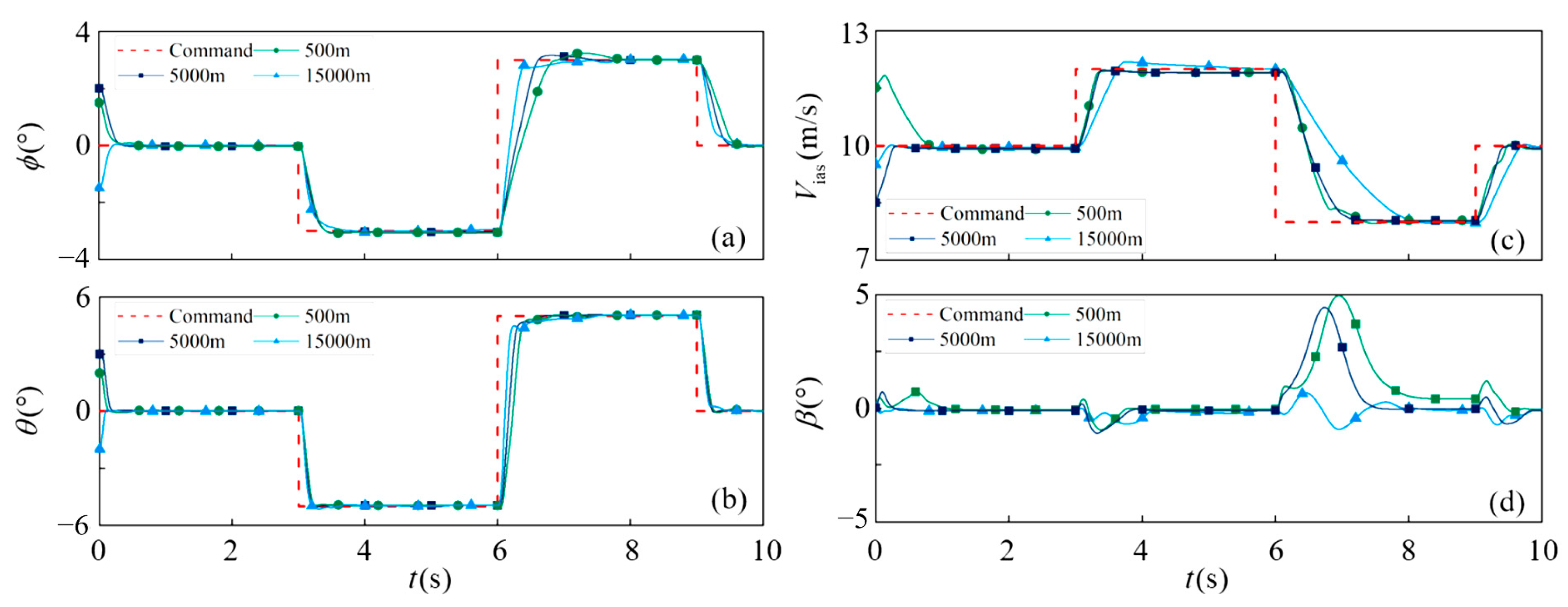
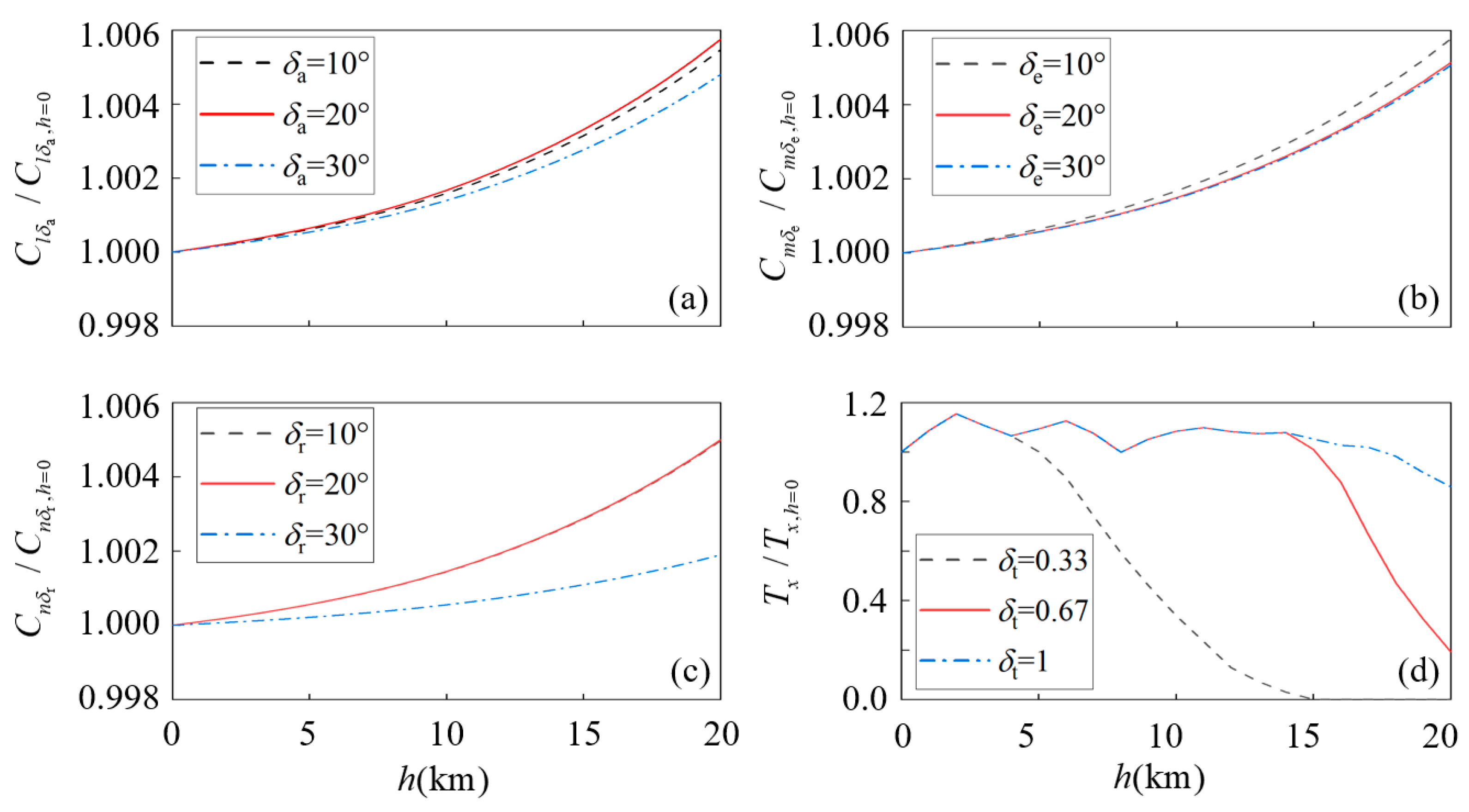
Figure 9 shows the time histories of the attitude in the digital model testing in which the initial state is randomly selected to track the doublet-wave target without perturbation or delay. In the different altitude cases at 500 m, 5000 m, and 15,000 m, neural network controllers successfully followed all the reference values. However, due to the influence of altitude on the efficiency of the aerodynamic and control surface, there are some differences in its dynamic performance. Figure 10 shows the variation trend of aerodynamic coefficients of various types of actuators at different altitudes, where the value at 0 km is set as the benchmark. It can be seen from Figure 10a–c that the contribution of various control surfaces to the moment increases with the increase in altitude, while from Figure 10d, the thrust provided by the propulsion system decreases. Therefore, the tracking speed of roll angle and pitch angle becomes faster, while the equivalent airspeed shows an opposite trend when altitude increases.

5.2. Results in Hardware-in-Loop Platform

In the present work, we pay more attention to the performance of the low-level attitude controller designed through reinforcement learning, so the Total Energy Control System (TECS) [26] and L1 guidance algorithm [32] are employed to generate pitch angle, roll angle attitude, and throttle commands as a high-level controller. The attitude commands, together with the necessary sensor signals, are transmitted to the neural network to calculate servo angles, while the throttle command calculated by the neural network is replaced by that obtained according to TECS in order to match the flight climb rate. All controllers operate at 25 Hz, which provides sufficient computation time for the neural network controller, even if each inference step only takes 2 ms.
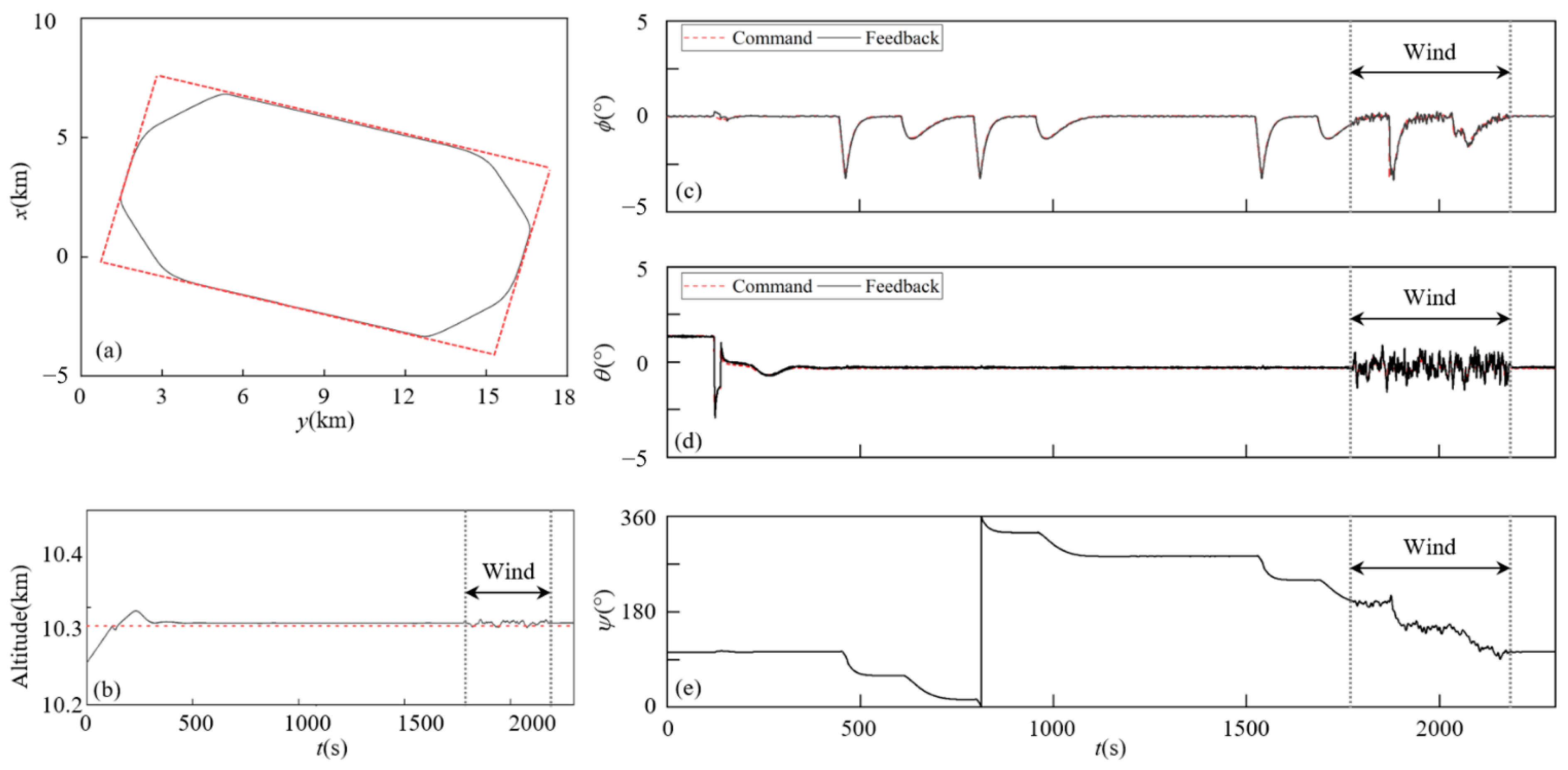
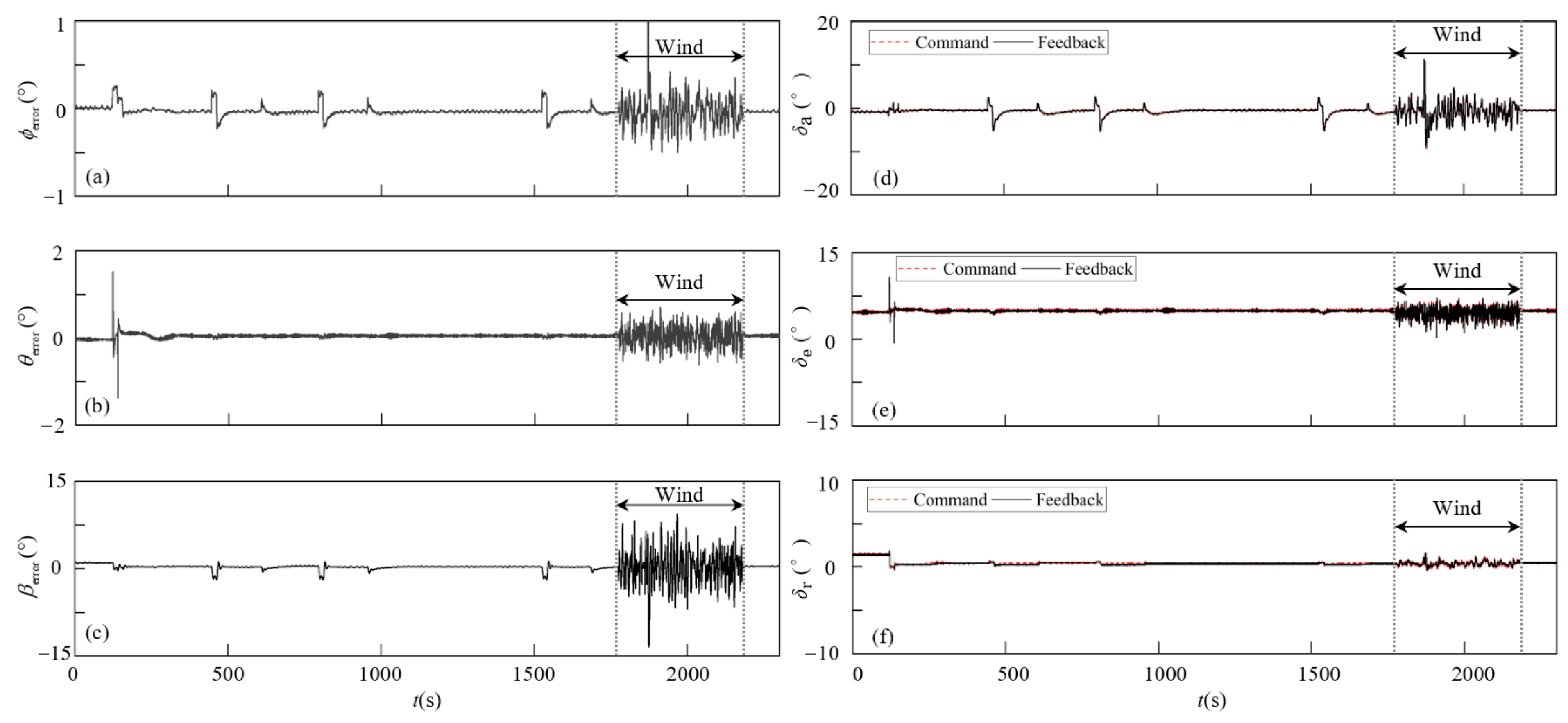
A rectangular route is set for the HIL verification, and the turbulent wind is simulated during the flight. The tracking process at 10 km altitude is shown in Figure 11a,b, during which its attitude angle commands and measured feedback are shown in Figure 11c–e. For a more accurate analysis of the tracking performance, the attitude commands are subtracted by the actual attitude feedback measured by the INS system to obtain the error diagram shown in Figure 12a–c, and the time histories of the corresponding control surface deflections are shown in Figure 12d–f. At the moment when the attitude command generates step changes, the tracking error will increase instantaneously due to the communication delay. The roll angle and sideslip angle react more slowly than the pitch angle. This phenomenon is caused by the fact that the aircraft is designed to have less sensitivity in transverse and directional motion than in longitudinal motion. In the level flight stage during the period of 1000 s–1500 s, the average absolute errors of attitude angle roll, pitch, and sideslip angles are 0.046°, 0.053°, and 0.3°, respectively.
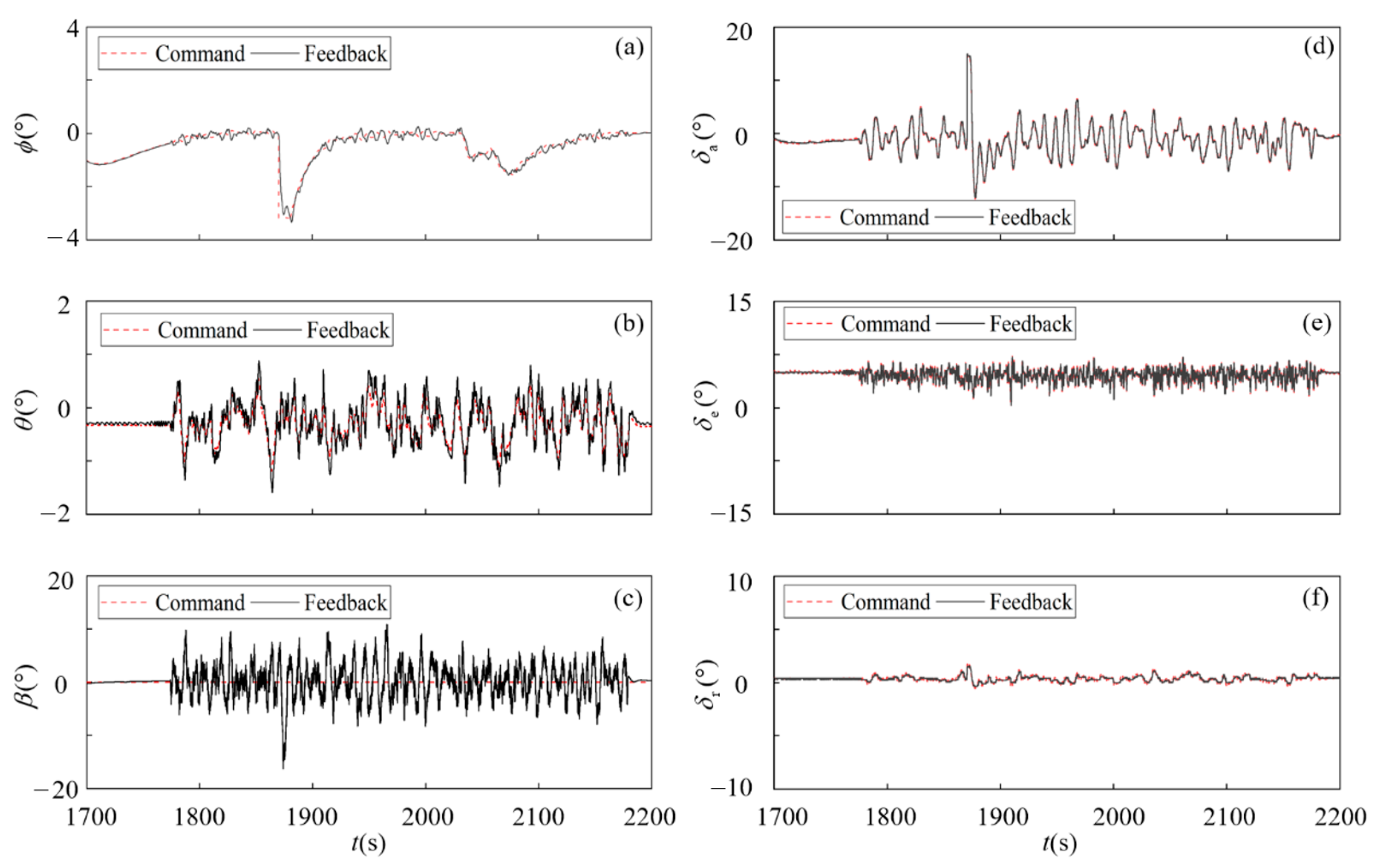
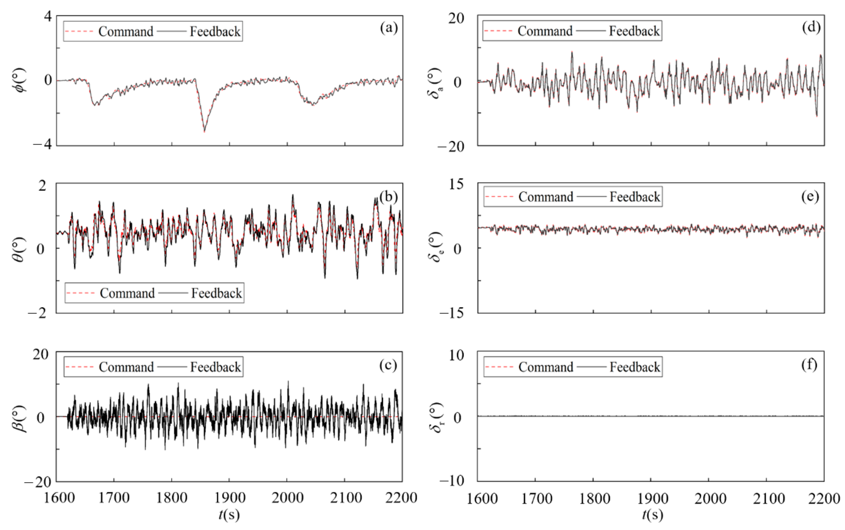
When facing the turbulence wind during the period of 1900 s–2300 s, the controller also responds quickly to changes in external commands to keep the vehicle stable, as shown in Figure 13. A gain-schedule PID controller is tuned as the traditional attitude tracking method for comparison, whose performance of anti-wind is shown in Figure 14. Both controllers are able to stay close to the reference values when following the dynamically changing commands but will fluctuate when affected by the turbulent wind. Here, Root Mean Square Errors (RMSE) is employed to evaluate the accuracy of attitude tracking, and a smooth metric S m [30] is used to describe the smoothness of the controller output:
S m = 1 n i = 1 n M i f i f s
where M i is the amplitude of the i th frequency component f i , and f s is the sampling frequency. A larger number indicates the presence of a larger high-frequency signal component, often indicating a more expensive drive, while a smaller number indicates a smoother response. Table 8 shows the comparison of the above two metrics between PID and NN. The neural network controller designed through RL only controls the attitude by output elevator, aileron, and rudder, so after learning the training scenario defined in Section 3, the RMSE of roll, pitch, and sideslip angles are still stable in the hardware-in-loop simulation environment of the wind field that has never been encountered. But it also sacrifices some of the smoothness of the actuators, such as the elevator. As expected, the combined coupling of airspeed and pitch channels is affected due to the mandatory shielding of the throttle control of the NN controller, making the RMSE of IAS more unstable. These results show that the attitude controller designed by reinforcement learning can not only be combined with any high-level module but can achieve similar performance with the traditional method in a shorter design time.

5.3. Adaptive Ability

The basic results in the previous section have shown the robustness of the NN controller to the difference in hardware delays, coding, and solver forms between the HIL verification and training process, which can also be considered as a gap in the dynamic performance of the system. Further, the adaptive ability of the neural network controller is examined by changing the model parameters in the hardware-in-loop simulation. In Section 3.4, the “positive perturbation” condition represents that the aircraft model parameters are deviated from the reference to make the overall performance of the aircraft more aggressive and positive. And the “negative perturbation” condition makes it clumsy and negative. At the same time, the response under the reference model ξ is also shown as a control group. The performance of the controller in the strict condition is explored by updating the model parameters each time before the semi-physical platform is turned on. Parameter perturbation in hardware-in-loop simulation verification are shown in Table 9.
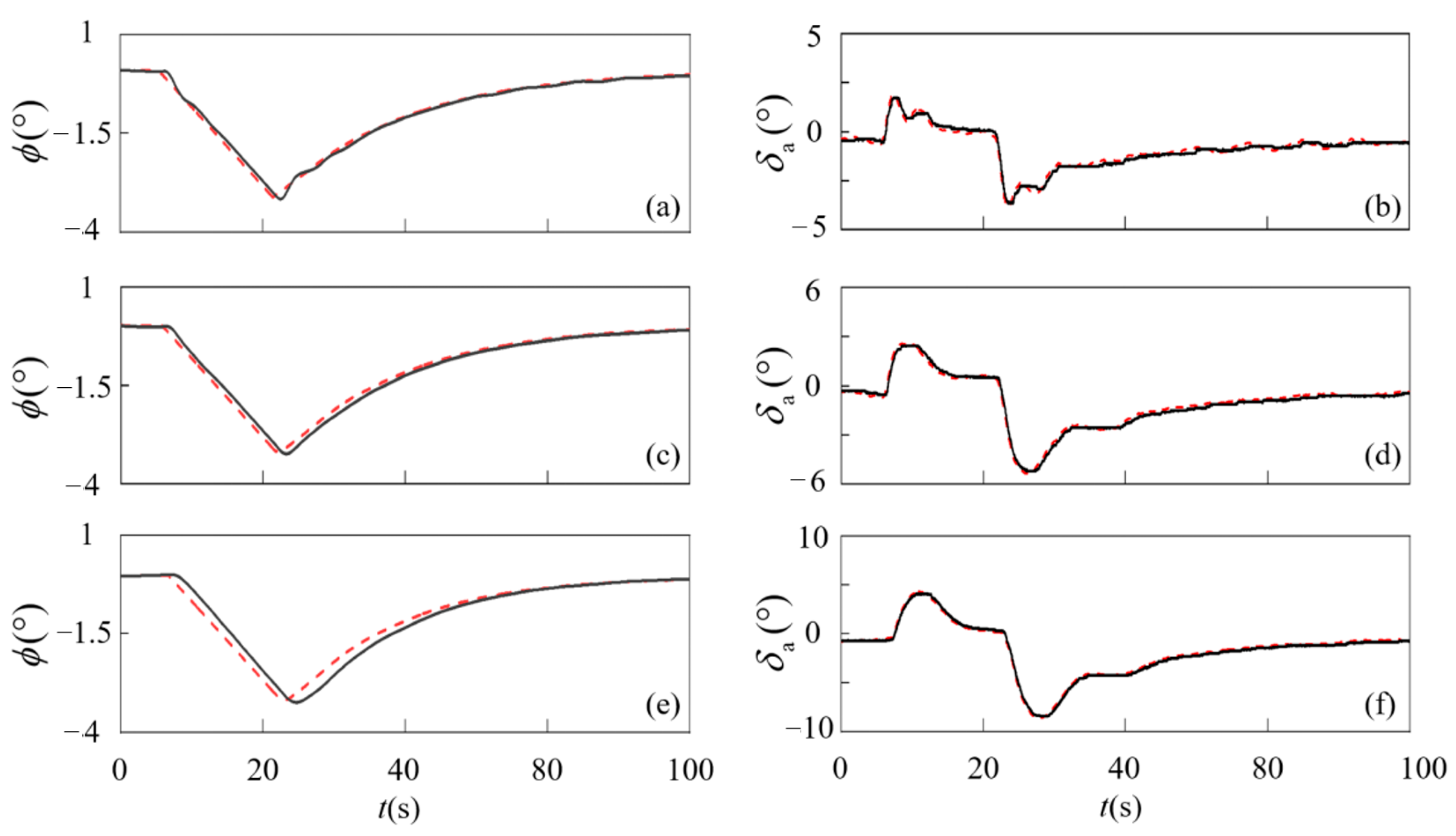
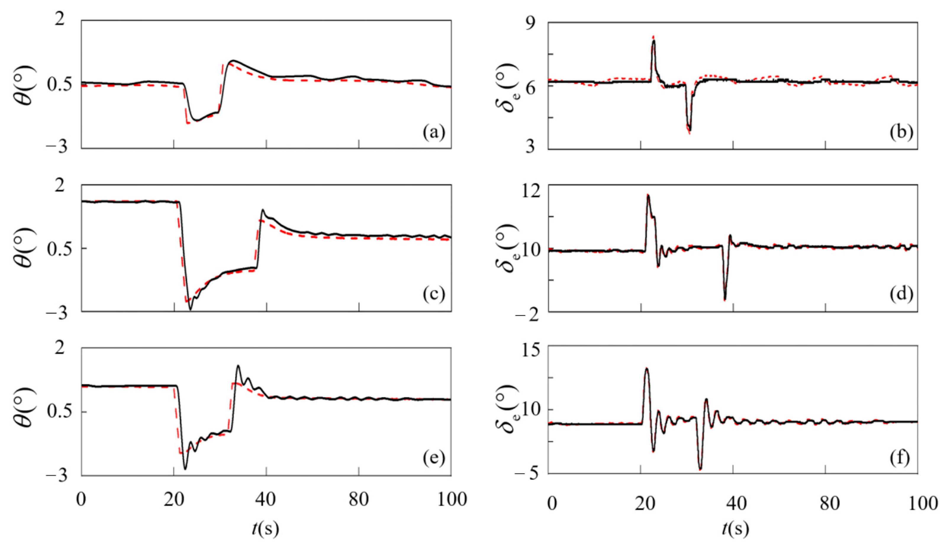
Figure 15 shows the curve of roll angle and aileron response, and Figure 16 shows the curve of pitch angle trend and elevator response under different conditions when the attitude setpoints change. As seen in Figure 15b,d,f, as the aircraft performance becomes increasingly clumsy, the aerodynamic efficiency of the control surface is reduced, and the steering gear deflection instruction calculated by the neural network controller also becomes bigger at the completion of the same attitude. At the same time, the following stance instruction also slows down in the dynamic process, as shown in Figure 16e. A similar phenomenon is shown in Figure 16, but rapid elevator changes also bring about overshooting and oscillation. This result matches that of the digital simulation presented in Figure 9. The neural network controller can adaptively change the control output according to the current state to follow the target instruction without receiving the parameters of the model, which is a benefit of the domain randomization in the training process. At the same time, the network structure of LSTM enables the controller to process the historical information of the time dimension, which further improves its adaptive ability.
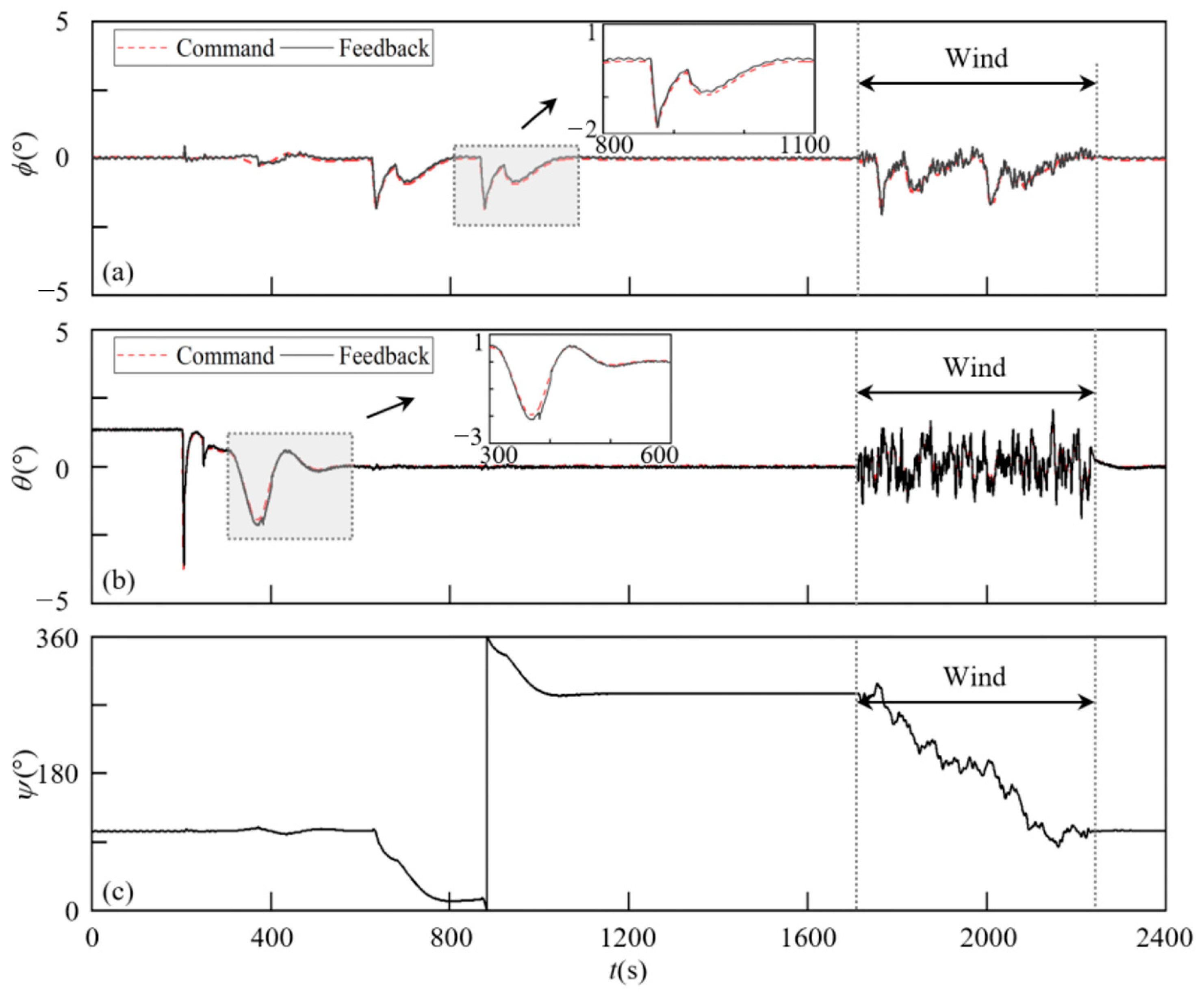
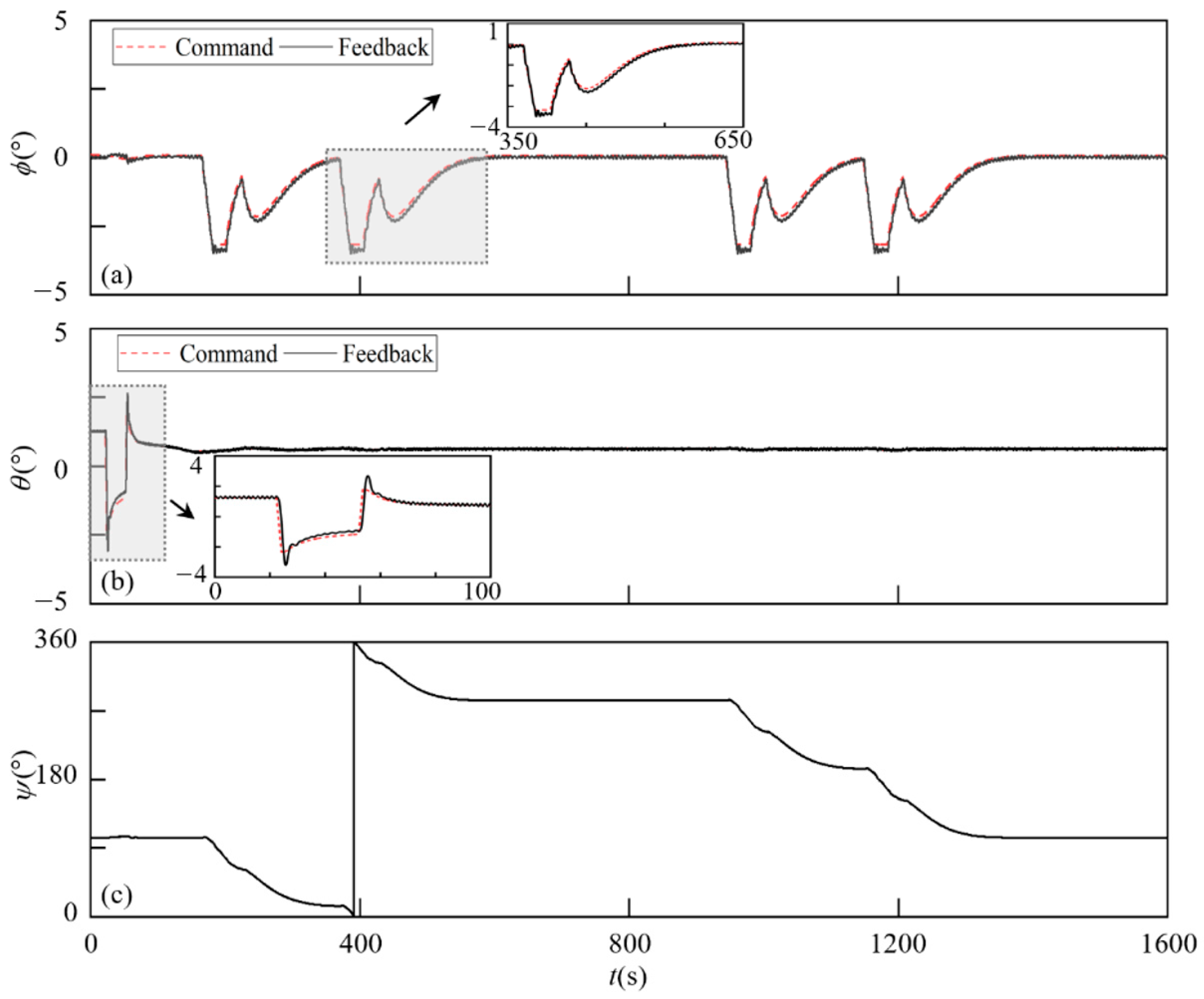
At the present stage, solar-powered UAV widely adopts energy management strategy based on potential energy storage in order to make full use of energy, so it needs to have flight control ability across 0–20 km altitude. Therefore, in addition to the above flight test at 10 km altitude, we also conducted the simulation test of hardware-in-loop at two typical altitudes of 1 km and 20 km, and the specific settings are the same as those in Section 5.2. Figure 17 shows the attitude change during the flight at 1 km altitude, and Figure 18 shows the content at 20 km altitude. Since the altitude of 20 km is already in the stratosphere, we did not introduce turbulent wind test conditions in the simulation process. It can be seen from the curve in the figure that the neural network controller can quickly and accurately follow the attitude command at low and high flight altitudes. For the level flight phase at the altitude of 1 km and 20 km, the steady-state error of bank angle is 0.03° and 0.04°, respectively, and the steady-state error of pitch angle is about 0.02° and 0.03°, respectively.

5.4. The Influence of Mechanical Difference

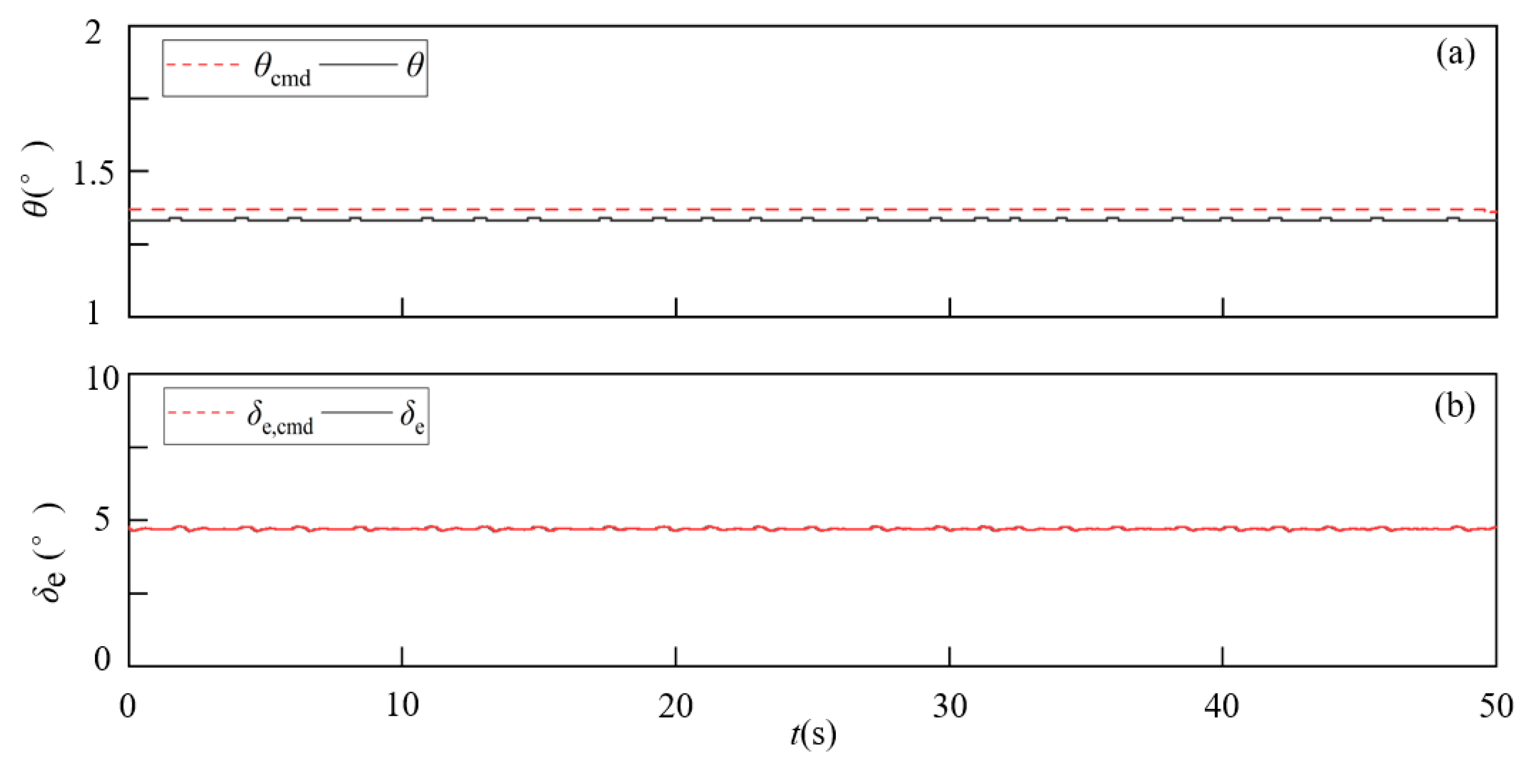
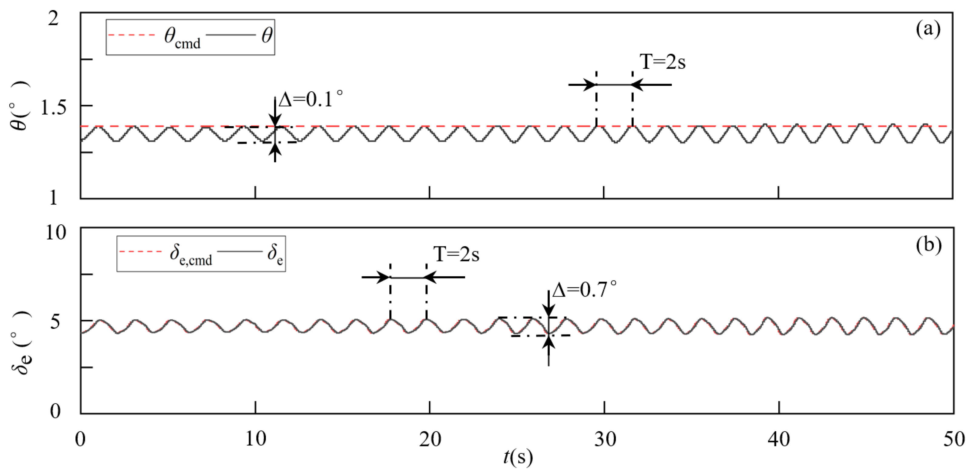
During the verification in the HIL platform, it was found that when tracking a constant angle command, the attitude feedback and the servo would have a small periodic fluctuation whether in the PID controller or the neural network controller. We speculate that the fundamental reason for this was caused by the dead zone of the steering gear. In this case, we use digital models to quantitatively explore the influence of the mechanical difference.
Firstly, we simulate the ideal steering gear model, that is, the command of the servo calculated by the neural network controller only passes through the first-order inertial dynamics model of the actuator described in Section 2.3, and then the calculated ideal response is directly used to solve the dynamics without connecting the real servos. The fragment of the flight process is shown in Figure 19.
Subsequently, we modeled the behavior of the steering gear system with backlash that the module implements a system in which a change in the input signal causes the output signal to change by the same amount, but the initial change in the input signal does not affect the output when the direction of the input signal changes [32]. The deadband width is set to 0.3°. Under this simulation setting, the servo angle calculated by the NN controller is first passed through the ideal backlash model, and then is used in the aircraft dynamics solution process after the digital model of the actuator, again without access to the real servo. The flight process in this case is shown in Figure 20. By comparing Figure 19 and Figure 20, the gap between ideal and reality caused by real equipment can be clearly seen. This gap causes the attitude of the aircraft to show small fluctuations around the steady-state value of the ideal situation in a long period but cannot be shaken off.

6. Conclusions

In the present work, a low-level neural network controller for solar-powered UAVs is trained through a reinforcement learning approach based on the Soft Actor-Critic algorithm. The control surface deflection and throttle of propellers are calculated by the current flight information and attitude command formulated by the high-level module in flight autopilot. In the design process, the gap between the digital model and real hardware was eliminated as much as possible by applying domain randomization to the parameters of the aircraft model and adding sensor and environmental noise.
In the developed real-time hardware-in-loop simulation platform, the neural network controller was deployed in an extra computer without re-training and communicated with flight autopilot through the serial port. The test platform involves a GNSS/INS system, servos, and airborne cable to make the simulation more realistic. By setting up a rectangular mission route and high-level control modules, the attitude tracking performance and anti-wind ability of the neural network controller are verified. At the same time, the robustness and adaptive ability of the controller under different heights and different model parameters are explored. The results in the HIL platform show that the neural network controller obtained by the reinforcement learning method training for simple step-style tasks can also complete complex continuous flight tasks never attempted before. Additionally, it has comparable performance with the well-tuned gain scheduling PID controller but it has a low workload.
In the future, this control method and neural network controller will be further verified and gradually transplanted into real flight experiments. At the same time, a safe switching logic and judgment method should be designed for backup controllers. Based on the existing methods, more ground flight verifications will be carried out to further verify the effectiveness of the proposed method. For instance, the energy generation is much lower than the energy consumption, which means additional weight. On the one hand, it means a change in the body mass, and on the other hand, it also brings conditions for the aircraft to perform more maneuvers. In subsequent research, we will explore the impact of these changes in energy and weight on the flight characteristics of solar-powered unmanned aerial vehicles with DRL controllers. The applicability research will be carried out for advanced aircraft such as flying-wing UAVs and cluster UAVs. This study will be applied AI to drone control, aiming to explore the feasibility of this approach. The experiment in this paper is relatively simple, and there are many problems worthy of further study. At present, the main difficulties restricting the application of reinforcement learning controllers are reliability and trustworthiness. The generalization ability of reinforcement learning is also worth further exploration. Compared with classical methods, we do not emphasize the advantages or disadvantages of reinforcement learning. We are just showing one possible exploration. Reinforcement learning, as a new controller, has important application potential in UAV control. As reinforcement learning advances in the future, UAV control challenges will undoubtedly be more effectively overcome.

Author Contributions

Conceptualization, B.Z. and X.M.; methodology, B.W.; software, H.C.; formal analysis, H.C.; investigation, Y.Y.; resources, B.W.; data curation, B.Z.; writing—original draft, Y.Y.; writing—review and editing, W.N.; visualization, Y.Y.; supervision, B.Z.; project administration, X.M.; funding acquisition, X.M. All authors have read and agreed to the published version of the manuscript.

Funding

Supported by the Taishan Scholars Program, grant number: tsqn202312319.

Data Availability Statement

The original contributions presented in the study are included in the article, further inquiries can be directed to the corresponding authors.

Conflicts of Interest

The authors declare no conflict of interest.

References

  1. Martin, R.A.; Gates, N.S.; Ning, A.; Hedengren, J.D. Dynamic optimization of high-altitude solar aircraft trajectories under station-keeping constraints. J. Guid. Control. Dyn. 2019, 42, 538–552. [Google Scholar] [CrossRef]
  2. Gao, X.Z.; Hou, Z.X.; Guo, Z.; Liu, J.X.; Chen, X.Q. Energy management strategy for solar-powered high-altitude long-endurance aircraft. Energy Convers. Manag. 2013, 70, 20–30. [Google Scholar] [CrossRef]
  3. Liu, X.; Sun, Q.; Cooper, J.E. LQG based model predictive control for gust load alleviation. Aerosp. Sci. Technol. 2017, 71, 499–509. [Google Scholar] [CrossRef]
  4. Cook, R.G.; Palacios, R.; Goulart, P. Robust gust alleviation and stabilization of very flexible aircraft. AIAA J. 2013, 51, 330–340. [Google Scholar] [CrossRef]
  5. Wang, Y.; Wynn, A.; Palacios, R. Model-predictive control of flexible aircraft dynamics using nonlinear reduced-order models. In Proceedings of the 57th AIAA/ASCE/AHS/ASC Structures, Structural Dynamics, and Materials Conference, San Diego, CA, USA, 4–8 January 2016; AIAA: Reston, VA, USA, 2016; p. 0711. [Google Scholar]
  6. Kim, T.; Kim, D.; Jeong, J.; Moon, S.; Kim, Y.; Bae, J.-S.; Park, S. A Study on the Development of Low-Altitude and Long-Endurance Solar-Powered UAV from Korea Aerospace University (2)-Flight Control and Guidance of Solar Powered UAV. J. Korean Soc. Aeronaut. Space Sci. 2022, 50, 479–487. [Google Scholar]
  7. Noll, T.E.; Brown, J.M.; Perez-Davis, M.E.; Ishmael, S.D.; Tiffany, G.C.; Gaier, M. Investigation of the Helios Prototype Aircraft Mishap Volume I Mishap Report; NASA: Washington, DC, USA, 2004. [Google Scholar]
  8. Weiser, C.; Ossmann, D. Baseline Flight Control System for High Altitude Long Endurance Aircraft. In Proceedings of the AIAA SCITECH 2022 Forum, San Diego, CA, USA and Online, 3–7 January 2022; p. 1390. [Google Scholar]
  9. Ye, D.; Chen, G.; Zhang, W.; Chen, S.; Yuan, B.; Liu, B.; Chen, J.; Liu, Z.; Qiu, F.; Yu, H.; et al. Towards playing full moba games with deep reinforcement learning. Adv. Neural Inf. Process. Syst. 2020, 33, 621–632. [Google Scholar]
  10. Silver, D.; Huang, A.; Maddison, C.J.; Guez, A.; Sifre, L.; van den Driessche, G.; Schrittwieser, J.; Antonoglou, I.; Panneershelvam, V.; Lanctot, M.; et al. Mastering the game of Go with deep neural networks and tree search. Nature 2016, 529, 484–489. [Google Scholar] [CrossRef] [PubMed]
  11. Antonova, R.; Cruciani, S.; Smith, C.; Kragic, D. Reinforcement learning for pivoting task. arXiv 2017, arXiv:1703.00472. [Google Scholar]
  12. Peng, X.B.; Andrychowicz, M.; Zaremba, W.; Abbeel, P. Sim-to-real transfer of robotic control with dynamics randomization. In Proceedings of the 2018 IEEE International Conference on Robotics and Automation(ICRA), Brisbane, Australia, 21–25 May 2018; IEEE: Piscataway, NJ, USA, 2018; pp. 3803–3810. [Google Scholar]
  13. Hoel, C.J.; Wolff, K.; Laine, L. Automated speed and lane change decision making using deep reinforcement learning. In Proceedings of the 2018 21st International Conference on Intelligent Transportation Systems (ITSC), Maui, HI, USA, 4–7 November 2018; IEEE: Piscataway, NJ, USA, 2018; pp. 2148–2155. [Google Scholar]
  14. Wang, B.L.; Gao, X.Z.; Xie, T. An evolutionary multi-agent reinforcement learning algorithm for multi-UAV air combat. Knowledge-Based Systems. Knowl.-Based Syst. 2024, 299, 112000. [Google Scholar] [CrossRef]
  15. Van, K.E.J.; Chu, Q.P.; Mulder, J.A. Continuous adaptive critic flight control aided with approximated plant dynamics. In Proceedings of the AIAA Guidance, Navigation, and Control Conference and Exhibit, Keystone, CO, USA, 21–24 August 2006; AIAA: Reston, VA, USA, 2006; p. 6429. [Google Scholar]
  16. Heyer, S.; Kroezen, D.; Van, K.E.J. Online adaptive incremental reinforcement learning flight control for a CS-25 class aircraft. In Proceedings of the AIAA Scitech 2020 Forum, Orlando, FL, USA, 6–10 January 2020; AIAA: Reston, VA, USA, 2020; p. 1844. [Google Scholar]
  17. Lambert, N.O.; Drew, D.S.; Yaconelli, J.; Levine, S.; Calandra, R.; Pister, K.S.J. Low-level control of a quadrotor with deep model-based reinforcement learning. IEEE Robot. Autom. Lett. 2019, 4, 4224–4230. [Google Scholar] [CrossRef]
  18. Wada, D.; Araujo-Estrada, S.A.; Windsor, S. Unmanned aerial vehicle pitch control using deep reinforcement learning with discrete actions in wind tunnel test. Aerospace 2021, 8, 18. [Google Scholar] [CrossRef]
  19. Kaufmann, E.; Bauersfeld, L.; Loquercio, A.; Müller, M.; Koltun, V.; Scaramuzza, D. Champion-level drone racing using deep reinforcement learning. Nature 2023, 620, 982–987. [Google Scholar] [CrossRef] [PubMed]
  20. Zheng, X.; Bao, C.; Lin, D.; Liu, C. Semi-Physical Simulation Design of UAV Simulation Training System. J. Phys. Conf. Ser. 2019, 1302, 022029. [Google Scholar] [CrossRef]
  21. Hu, Y.P.; Guo, J.; Meng, W.Y.; Liu, G.; Xue, W. Longitudinal Control for Balloon-Borne Launched Solar Powered UAVs in Near-Space. J. Syst. Sci. Complex. 2022, 35, 802–819. [Google Scholar] [CrossRef]
  22. Beard, R.W.; McLain, T.W. Small Unmanned Aircraft: Theory and Practice; Princeton University Press: Oxford, UK, 2012; pp. 39–58. [Google Scholar]
  23. Sissenwine, N.; Dubin, M.; Wexler, H. The US standard atmosphere, 1962. J. Geophys. Res. 1962, 67, 3627–3630. [Google Scholar] [CrossRef]
  24. Dryden Wind Turbulence Model (Continuous) [Internet]. MATHWORKS. [Updated 18 February 2019]. Available online: https://se.mathworks.com/help/aeroblks/drydenwindturbulencemodelcontious.html (accessed on 15 November 2022).
  25. Bøhn, E.; Coates, E.M.; Moe, S.; Johansen, T.A. Deep reinforcement learning attitude control of fixed-wing UAVs using proximal policy optimization. In Proceedings of the International Conference on Unmanned Aircraft Systems (ICUAS), Atlanta, GA, USA, 11–14 June 2019; IEEE: Piscataway, NJ, USA, 2019; pp. 523–533. [Google Scholar]
  26. Kastner, N.; Looye, G. Generic tecs based autopilot for an electric high altitude solar powered aircraft. In Proceedings of the CEAS EuroGNC, Delft, The Netherlands, 10–12 April 2013. [Google Scholar]
  27. Haarnoja, T.; Zhou, A.; Abbeel, P.; Hartikainen, K.; Tucker, G.; Ha, S.; Tan, J.; Kumar, V.; Zhu, H.; Gupta, A.; et al. Soft actor-critic algorithms and applications. arXiv 2018, arXiv:1812.05905. [Google Scholar]
  28. Hochreiter, S.; Schmidhuber, J. Long short-term memory. Neural Comput. 1997, 9, 1735–1780. [Google Scholar] [CrossRef] [PubMed]
  29. Kingma, D.; Ba, J. Adam: A method for stochastic optimization. arXiv 2014, arXiv:1412.6980. [Google Scholar]
  30. Mysore, S.; Mabsout, B.; Mancuso, R.; Saenko, K. Regularizing action policies for smooth control with reinforcement learning. In Proceedings of the 2021 IEEE International Conference on Robotics and Automation (ICRA), Xi’an, China, 30 May–5 June 2021; IEEE: Piscataway, NJ, USA, 2021; pp. 1810–1816. [Google Scholar]
  31. Lillicrap, T.P.; Hunt, J.J.; Pritzel, A.; Heess, N.; Erez, T.; Tassa, Y.; Silver, D.; Wierstra, D. Continuous control with deep reinforcement learning. arXiv 2015, arXiv:1509.02971. [Google Scholar]
  32. Backlash [Internet]. MATHWORKS. Available online: https://ww2.mathworks.cn/help/simulink/slref/backlash.html?lang=en (accessed on 15 November 2022).
Figure 1. Solar-powered UAV designed by the authors’ team.
Drones 08 00428 g001
Figure 2. The responses obtained from mathematical servo model and real servo: (a) mathematical servo model, (b) real servo.
Drones 08 00428 g002
Figure 3. Classical flight control architecture [26].
Drones 08 00428 g003
Figure 4. The architecture of policy neural network.
Drones 08 00428 g004
Figure 5. Schematic diagram of simulation environment composition.
Drones 08 00428 g005
Figure 6. Signal pathway of the hardware-in-loop simulation platform.
Drones 08 00428 g006
Figure 7. Experimental setup diagram.
Drones 08 00428 g007
Figure 8. The recorded curve during training, where (a) is the simulation steps of one evaluation episode, and (b) is the normalized total reward of one episode.
Drones 08 00428 g008
Figure 9. The time histories of the attitude evaluated under the mathematical model: (a) ϕ, (b) Vias, (c) θ, (d) β.
Drones 08 00428 g009
Figure 10. The normalized actuator efficiency trends with altitude when Veas = 10 m/s.
Drones 08 00428 g010
Figure 11. The flight process at 10 km altitude: (a) x, (b) Altitude, (c) ϕ, (d) θ, (e) Ψ.
Drones 08 00428 g011
Figure 12. The attitude tracking errors and actuator changes at 10 km altitude: (a) ϕerror, (b) θerror, (c) βerror, (d) δa, (e) δe, (f) δr.
Drones 08 00428 g012
Figure 13. Enlarged view of flight process controlled by NN in the wind at 10 km altitude: (a) ϕ, (b) θ, (c) β, (d) δa, (e) δe, (f) δr.
Drones 08 00428 g013
Figure 14. Enlarged view of flight process controlled by PID in the wind at 10 km altitude: (a) ϕ, (b) θ, (c) β, (d) δa, (e) δe, (f) δr.
Drones 08 00428 g014
Figure 15. Roll angle and aileron response under different parameter perturbations: (a,b) are under positive perturbation, (c,d) are under reference model, and (e,f) are under negative perturbation. The red dashed lines represent the command values, and the black solid lines represent the real response.
Drones 08 00428 g015
Figure 16. Pitch angle and elevator response under different parameter perturbations: (a,b) are under positive perturbation, (c,d) are under reference model, and (e,f) are under negative perturbation. The red dashed lines represent the command values, and the black solid lines represent the real response.
Drones 08 00428 g016
Figure 17. The attitude tracking process for the route at 1 km altitude: (a) ϕ, (b) θ, (c) Ψ.
Drones 08 00428 g017
Figure 18. The attitude tracking process for the route at 20 km altitude: (a) ϕ, (b) θ, (c) Ψ.
Drones 08 00428 g018
Figure 19. Flight process under the ideal servo model: (a) θ, (b) δe.
Drones 08 00428 g019
Figure 20. Flight process under the ideal servo model with backlash: (a) θ, (b) δe.
Drones 08 00428 g020
Table 1. Basic parameters of the studied aircraft.
VariablesDescriptionValue
m ( kg ) Total mass359
S ( m 2 ) Wing area78.5
AR Aspect ratio15.6
b ( m ) Wing span35
c ( m ) Wing chord2.27
I ( kg m ) Moment of inertia matrix 15221 0 37 0 1827.5 0 37 0 16967
Table 2. Ranges of attitude and action commands.
ParametersDescriptionRange
ϕ cmd ( ° ) Target roll angle[−5, 5]
θ cmd ( ° ) Target pitch angle[−10, 10]
V eas , cmd ( m / s ) Target equivalent airspeed[8, 12]
δ a c ( ° ) Aileron deflection angle command[−30, 30]
δ e c ( ° ) Elevator deflection angle command[−30, 30]
δ r c ( ° ) Rudder deflection angle command[−20, 20]
δ t c ( ° ) Throttle command for propellers[0, 1]
Table 3. The variance σ m in OU noise for different state elements.
ParametersValueUnit
z 0m
ϕ , θ , ψ 0.001rad
p , q , r 0.001rad/s
V eas 0.01m/s
α , β 0.001rad
δ a , δ e , δ r , δ t 0rad
Table 4. Domain randomization parameters during training. ξ denotes the basic reference value.
ParametersDescriptionDistribution
I Moment of inertia U ( 0.95 ξ , 1.15 ξ )
C L 0 , C L β , C L δ e , C L δ a , C L δ r , C L q Aerodynamic lift coefficients U ( 0.8 ξ , 1.2 ξ )
C D 0 , C D β , C D δ a , C D δ e , C D δ r Aerodynamic drag coefficients U ( 0.8 ξ , 1.2 ξ )
C Y β , C Y δ a , C Y δ r , C Y p , C Y q Lateral force coefficients U ( 0.8 ξ , 1.2 ξ )
C l β , C l δ a , C l δ r Roll moment coefficients U ( 0.8 ξ , 1.2 ξ )
C m 0 , C m β , C m δ e , C m δ a , C m δ r Pitching moment coefficients U ( 0.8 ξ , 1.2 ξ )
C n β , C n δ a , C n δ r Yaw moment coefficients U ( 0.8 ξ , 1.2 ξ )
C l p , C l r , C m q , C n p , C n r Damping and cross derivative U ( 0.8 ξ , 1.2 ξ )
Table 5. The operating data and performance of the GNSS/INS system.
IndexRollPitchYaw
Sampling frequency100 Hz
Measuring range of rate−200°/s~+200°/s
Measuring range of angle−180°~+180°Measuring range of angle−180°~+180°
Measuring accuracy of angle≤0.1°Measuring accuracy of angle≤0.1°
Table 6. The operating data and performance of the three-axis turntable.
IndexRollPitchYaw
Range of measuring angleNo limit
Measuring accuracy of angle±0.001°
Repeatability accuracy of angle±0.0005°
Resolution of angle±0.0001°
Range of rated speed±2500°/sRange of rated speed±2500°/s
Resolution at rated speed0.0001°/sResolution at rated speed0.0001°/s
Table 7. The operating data and performance of the used servo.
IndexRoll
Max. speed without load230°/s
Rated speed150°/s
Default travel angle±45°
Max. travel angle±85°
Backlash (mechanical)≤0.5°
Table 8. The comparison of accuracy and smoothness between PID and NN. The better terms are bolded.
Controller RMSE ( ϕ ) RMSE ( θ ) RMSE ( V eas ) RMSE ( β ) S m ( δ a ) S m ( δ e ) S m ( δ r ) S m ( δ t )
PID0.1250.1930.3932.9159.50 × 10−54.48 × 10−50.00 × 10−51.12 × 10⁻⁵
RL0.0730.0840.4480.9563.03 × 10−56.63 × 10−51.05 × 10−51.27 × 10⁻⁵
Table 9. Parameter perturbation in hardware-in-loop simulation verification. The notation is inherited from Table 4.
ParametersPositiveNegative
I 0.95 ξ 1.05 ξ
C L 0 , C L β , C L δ e , C L δ a , C L δ r , C L q 1.10 ξ 0.90 ξ
C D 0 , C D β , C D δ a , C D δ e , C D δ r 0.90 ξ 1.10 ξ
C Y β , C Y δ a , C Y δ r , C Y p , C Y q 1.15 ξ 0.85 ξ
C l β , C l δ r , C m 0 , C m β , C m δ a , C m δ r , C n δ a , C n β , C n δ a , 0.85 ξ 1.15 ξ
C m δ e , C l δ a , C n δ r 1.15 ξ 0.85 ξ
C l p , C l r , C m q , C n p , C n r 0.7 ξ 1.30 ξ
Disclaimer/Publisher’s Note: The statements, opinions and data contained in all publications are solely those of the individual author(s) and contributor(s) and not of MDPI and/or the editor(s). MDPI and/or the editor(s) disclaim responsibility for any injury to people or property resulting from any ideas, methods, instructions or products referred to in the content.