A Multi-Waypoint Motion Planning Framework for Quadrotor Drones in Cluttered Environments

Abstract

In practical missions, quadrotor drones frequently face the challenge of navigating through multiple predetermined waypoints in cluttered environments where the sequence of the waypoints is not specified. This study presents a comprehensive multi-waypoint motion planning framework for quadrotor drones, comprising multi-waypoint trajectory planning and waypoint sequencing. To generate a trajectory that follows a specified sequence of waypoints, we integrate uniform B-spline curves with a bidirectional A* search to produce a safe, kinodynamically feasible initial trajectory. Subsequently, we model the optimization problem as a quadratically constrained quadratic program (QCQP) to enhance the trackability of the trajectory. Throughout this process, a replanning strategy is designed to ensure the traversal of multiple waypoints. To accurately determine the shortest flight time waypoint sequence, the fast marching (FM) method is utilized to efficiently establish the cost matrix between waypoints, ensuring consistency with the constraints and objectives of the planning method. Ant colony optimization (ACO) is then employed to solve this variant of the traveling salesman problem (TSP), yielding the sequence with the lowest temporal cost. The framework’s performance was validated in various complex simulated environments, demonstrating its efficacy as a robust solution for autonomous quadrotor drone navigation.

1. Introduction

In real-world scenarios such as inspection, surveying, and monitoring tasks, quadrotor drones frequently encounter the need to execute complex missions that involve navigating through multiple waypoints rather than simply targeting a single point. These tasks demand quadrotor drones to navigate safely through cluttered environments while minimizing travel time, where the sequence of waypoints is often not predetermined. Furthermore, multi-waypoint trajectory planning requires quadrotor drones to consider the spatial relationships between these waypoints. Navigation algorithms designed for single-goal navigation may introduce unnecessary path redundancy when applied to multi-waypoint trajectory planning problems, resulting in a waste of time and energy resources. Therefore, efficiently determining the optimal sequence for traversing waypoints and subsequently generating safe trajectories with minimal flight times pose a significant challenge.

Therefore, this paper proposes an advanced quadrotor multi-waypoint motion planning framework, as illustrated in Figure 1. For the multi-waypoint trajectory planning problem, we consider the spatial relationships between waypoints and propose a velocity-adaptive trajectory generation method based on uniform B-spline curves. This method utilizes the bidirectional A* method to obtain a sequence of B-spline control points, generating a kinodynamically feasible initial trajectory. Subsequently, we further optimize the smoothness of the trajectories using quadratically constrained quadratic programming (QCQP), enhancing trajectory trackability and reducing energy consumption. Finally, during the trajectory generation process, we employ a replanning approach to reduce the number of control point variables solved by QCQP, thus improving numerical stability and algorithm real-time performance. To determine the waypoint sequence in this variant of the traveling salesman problem (TSP), we employ a combination of the fast marching (FM) method and ant colony optimization (ACO). First, we compute the velocity map while adhering to the constraints of the proposed planning method. Then, we utilize FM to establish a time cost matrix between every pair of waypoints in the TSP problem. Finally, ACO is utilized to find the waypoint sequence with the lowest time cost.

We summarize our contributions as follows:

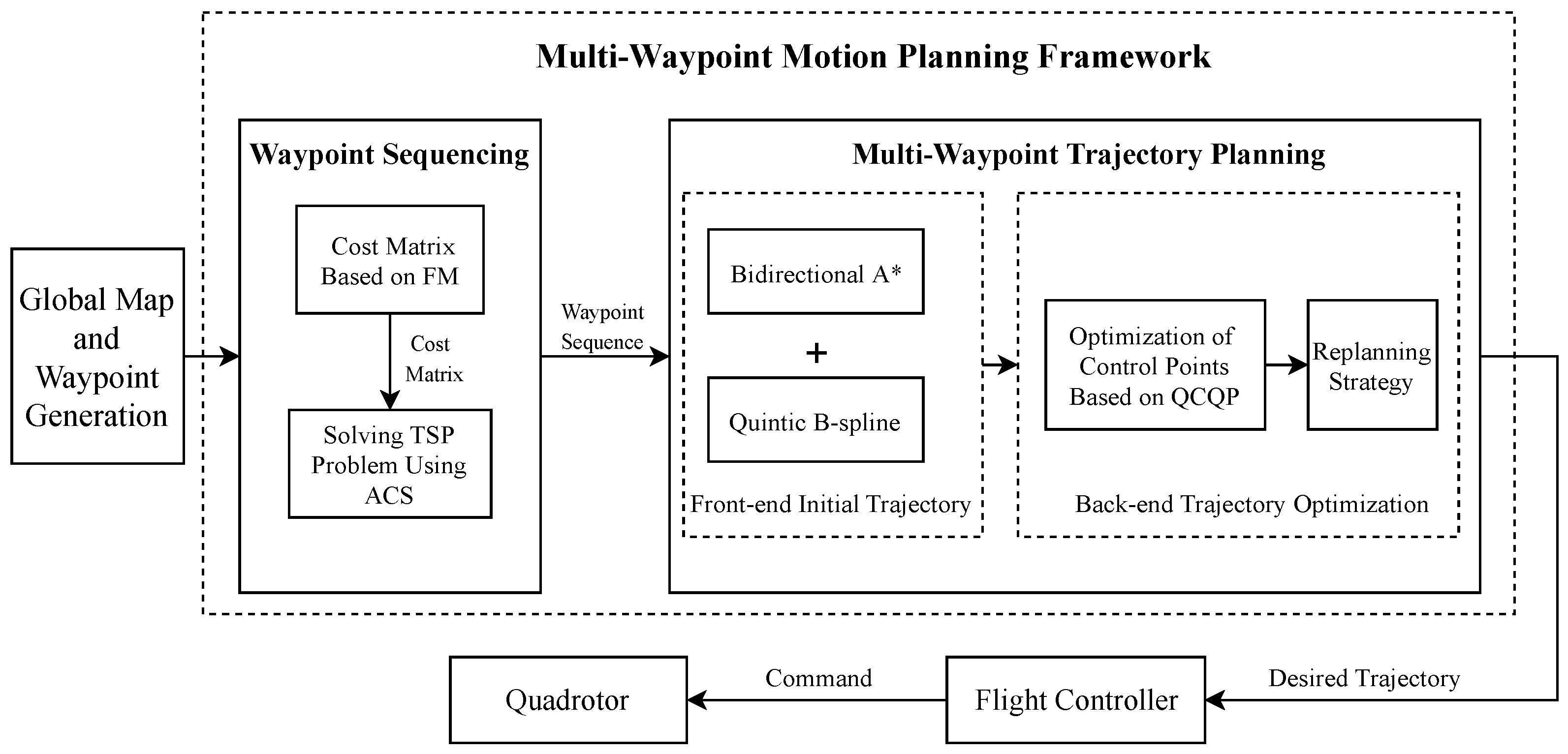
• We design a multi-waypoint trajectory planning method. We refine the bidirectional A* method with kinodynamic constraints, framing trajectory generation as a B-spline control point placement problem to achieve initial kinodynamically feasible trajectories, and QCQP is used to optimize the coordinates of the control points. During this process, the MINVO-based generation of the minimum convex hull of B-spline curves is employed to enlarge the solution space and avoid overly conservative trajectories.
• We design a method for determining waypoint sequences. While maintaining consistency with the objectives and constraints of multi-waypoint trajectory planning, we utilize the FM method to establish a cost matrix. ACO is then applied to solve this variant of TSP, yielding the waypoint sequence with the shortest time.
• We propose a multi-waypoint motion planning framework incorporating the aforementioned two components. We validate the effectiveness of our proposed method and this framework through extensive simulation experiments.

This paper is structured as follows. Section 2 reviews the related work. Section 3 introduces the proposed trajectory planning method, while Section 4 presents the proposed waypoint sequencing method. Section 5 presents the experimental results, followed by the discussion in Section 6 and conclusions in Section 7.

2. Related Works

Due to the differential flatness of quadrotor drones, their entire state can be represented by four flat outputs, with the most widely used being 3D position and yaw angle. The trajectory generation problem for quadrotors is also transformed into a problem of generating time-parameterized curves [1].

In the realm of quadrotor trajectory planning, a hierarchical planning framework is commonly utilized, which involves front-end path searching and back-end trajectory generation. The front-end search comprises search-based and sampling-based methods. Among the search-based approaches, A* [2] and its variations are extensively studied, while popular sampling-based techniques include RRT [3] and PRM [4]. However, these methods typically generate piecewise-linear paths, rendering them unsuitable for direct execution by quadrotor controllers. Consequently, back-end trajectory generation is essential to convert them into time-parameterized curves, such as polynomial curves [5], Bezier curves [6], and B-spline curves [7,8].

However, classical front-end path searching methods focus solely on obstacle avoidance, disregarding the dynamic characteristics of quadrotors. Consequently, the initial paths obtained from front-end path searching may not belong to the same homotopy class as the optimal trajectory in practice. In some cases, they may even fail to produce dynamically feasible trajectories through back-end trajectory generation, resulting in planning failures. Therefore, some scholars integrate the dynamic properties of quadrotors into the front-end path searching process. Reference [9] proposed a kinodynamic search method based on motion primitives, representing the motion dynamic constraints of quadrotors as motion primitives. Then, a graph search method similar to A* was employed to generate a kinodynamically feasible, continuous, and safe trajectory. Reference [7] introduced a search method considering motion dynamics based on the hybrid-state A* algorithm. After generating dynamically feasible initial trajectories, B-spline curves were used to fit and optimize the initial trajectories, further enhancing trajectory smoothness and safety. Reference [8] considered dynamical feasibility using the A* algorithm. By combining B-spline curves, the trajectory generation problem is transformed into a problem of placing B-spline control points. After generating a feasible sequence of control points, QCQP is used to optimize the positions of control points further, thereby improving trajectory smoothness.

Nevertheless, most trajectory planning algorithms are designed for single-goal navigation problems, with fewer algorithms tailored explicitly for multi-waypoint trajectory planning. Compared to single-goal problems, multi-waypoint problems must consider the spatial relationships between different waypoints to generate efficient trajectories. Reference [10] applied B-spline curves to trajectory generation involving multiple waypoints, resulting in shorter and smoother trajectories. However, its flight corridor is predefined and relatively narrow, suitable only for scenarios without obstacles between waypoints. Reference [11] considered the complete quadrotor flight model and proposed an optimization-based multi-waypoint trajectory generation method, aiming to obtain the optimal trajectory in terms of time. However, it did not account for the influence of obstacles. Reference [12] also considered the complete quadrotor model and adopted a hierarchical optimization approach. It first used a variant of PRM to obtain homotopy classes of paths, then guided the trajectory planning of the point-mass model using these homotopy classes, finally using the SST algorithm to plan multi-waypoint trajectories using the complete quadrotor model. Although this method considered obstacles, it suffered from the drawback of excessive computation times, making it unsuitable for real-time planning.

For the problem of finding the optimal waypoint sequence in terms of time, scholars have regarded it as a variant of the traveling salesman problem (TSP) [13,14,15,16]. Reference [13] addressed the problem of determining the sequence of multiple target points for autonomous underwater vehicles (AUVs) in complex underwater environments. Based on the A* algorithm, it utilized a path planning method combining coarse-grained modeling and fine-grained modeling to establish a cost matrix and solved the TSP problem using ACO to obtain the shortest path sequence of waypoints. Reference [14] proposed a method combining the adaptive weighted PRM (AWPRM) and the best ant colony system (BACS) to solve the problem of multi-quadrotor waypoint assignment and sequence determination. It used the Dubins method to construct the shortest obstacle-avoiding paths with turn radius constraints but did not consider additional quadrotor dynamic constraints. Both methods aim to minimize distance. Hence, the waypoint sequences obtained may not necessarily be the time-optimal solution after back-end trajectory generation. Reference [15] proposed a solution for the shortest time in multi-region quadrotor surveillance problems, but it required quadrotor drones to fly at maximum speed between multiple regions, which is unrealistic, as it did not consider the dynamic characteristics of quadrotors. The fast marching (FM) method is also employed to calculate the distance costs between multiple task points, which are then optimized using a genetic algorithm (GA) [16]. However, since they do not account for the robot’s dynamic characteristics when creating the speed map, it only determines the shortest distance sequence of task points using FM and GA, which does not correspond to the objective of minimizing time in practical tasks. Therefore, to achieve the shortest time waypoint sequence, it is essential to maintain consistency between the constraints of the waypoint sequencing method and the trajectory planning method. This consistency allows for the establishment of a cost matrix that more accurately reflects actual flight times, thereby yielding a more optimal solution.

3. B-Spline-Based Bidirectional A* Trajectory Planning

This paper proposes a hierarchical multi-waypoint trajectory planning method for a given sequence of waypoints. The method comprises a front-end search integrating bidirectional A* and B-spline curves and back-end optimization using quadratically constrained quadratic programming (QCQP). The front-end search transforms the initial trajectory generation problem into a B-spline control point placement problem. By integrating motion dynamic constraints, an improved bidirectional A* algorithm is employed to obtain a sequence of control points that meet the requirements. Consequently, a safe initial trajectory that satisfies the motion dynamic constraints is generated. In the back-end optimization, QCQP is employed to further optimize the positions of the control points, resulting in smoother and more energy-efficient trajectories. Finally, in response to the challenge of optimizing a large number of waypoints, a replanning strategy is utilized to improve the real-time performance of trajectory planning and the numerical stability of QCQP.

3.1. B-Spline Curves

B-spline curves are piecewise polynomial curves. For a B-spline curve of degree k, it is determined by a knot vector $[t_0,t_1\cdots t_{n+k+1}]$ and control points $[{\mathit{q}}_0,{\mathit{q}}_1\cdots {\mathit{q}}_n]$ together. The computation method is as follows:

$$\mathit{x}\left(t\right)=\sum _{i=0}^n{\mathit{q}}_i{B}_{i,k}\left(t\right)$$

(1)

$$B_{i,0}\left(t\right)=\left\{\begin{array}{cc}1,\hfill & t_i\le t<t_{i+1}\hfill \\ 0,\hfill & \mathrm{otherwise}\hfill \end{array}\right.$$

(2)

$$B_{i,k}\left(t\right)={\displaystyle \frac{t-t_i}{t_{i+k}-t_i}}{B}_{i,k-1}\left(t\right)+{\displaystyle \frac{t_{i+k+1}-t}{t_{i+k+1}-t_{i+1}}}{B}_{i+1,k-1}\left(t\right)$$

(3)

where $t\in [t_i,t_{i+1})$ is the interval when the basis function $B_{i,k}\left(t\right)$ is nonzero. This indicates that the B-spline curve in $t\in [t_i,t_{i+1})$ is solely determined by the local $k+1$ control points $[{\mathit{q}}_i,{\mathit{q}}_{i+1}\cdots {\mathit{q}}_{i+k}]$. This property is known as the local control characteristic of B-spline curves, and the B-spline curve in $t\in [t_i,t_{i+1})$ lies entirely within the convex hull formed by $[{\mathit{q}}_i,{\mathit{q}}_{i+1}\cdots {\mathit{q}}_{i+k}]$.

Figure 2 shows where the local quintic B-spline trajectory (red curve) lies within the convex hull formed by six local control points (cyan–blue area). Additionally, B-spline curves also possess derivative properties, meaning the derivative of a B-spline curve remains a B-spline curve.

The unique properties of B-spline curves confer distinct advantages in obstacle avoidance and dynamic constraints. Regarding obstacle avoidance, the convex hull property of B-spline curves ensures that the convex hull formed by control points satisfies the obstacle avoidance constraints when located in obstacle-free regions. Dynamic constraints are typically defined by the maximum values of the quadrotor drone’s velocity and acceleration, denoted as $v_{max}$ and $a_{max}$, respectively. Leveraging the derivative characteristics, low-order B-spline curves (velocity and acceleration curves) are derived. Subsequently, by utilizing the convex hull property, control points $v_i$ and $a_i$ of the velocity and acceleration curves are constrained not to exceed their maximum values, thereby ensuring dynamic feasibility.

Due to the significant influence of the intermediate two B-spline control points on the local curve, for a quintic B-spline curve, the local control points ${\mathbf{Q}}_i={[{\mathit{q}}_i,{\mathit{q}}_{i+1}\cdots {\mathit{q}}_{i+5}]}^{\top }$ generate the i-th segment trajectory near the line connecting ${\mathit{q}}_{i+2}$ and ${\mathit{q}}_{i+3}$. It provides favorable conditions for using A* search: ensuring that the line connecting ${\mathit{q}}_{i+2}$ and ${\mathit{q}}_{i+3}$ does not intersect with obstacles, it can be approximately assumed that the i-th segment B-spline curve will not collide with obstacles [8].

However, in practical applications, the convex hull formed by the control points of the B-spline curve does not tightly enclose the local segments of the curve. Consequently, requiring the convex hull to be within the feasible region will result in conservative trajectories. Therefore, we use control points generated by the MINVO basis [17] to replace the B-spline control points, minimizing the volume of the convex hull and producing more aggressive trajectories.

As shown in Figure 3, it can be observed that compared to the local B-spline control points ${\mathbf{Q}}_{bs}$, the convex hull formed by the MINVO control points ${\mathbf{Q}}_{mv}$ can more tightly envelop the local B-spline curve. Therefore, in the process of verifying dynamic feasibility, we use ${\mathbf{Q}}_{mv}$ instead of ${\mathbf{Q}}_{bs}$ for feasibility checks. These two can be converted into each other through matrix operations:

$$\mathit{p}\left(\mathit{s}\left(t\right)\right)=\mathit{s}{\left(t\right)}^{\top }{\mathbf{M}}_{bs6}{\mathbf{Q}}_{bs}=\mathit{s}{\left(t\right)}^{\top }{\mathbf{M}}_{mv6}{\mathbf{Q}}_{mv}$$

(4)

$${\mathbf{Q}}_{mv}={\left({\mathbf{M}}_{mv6}\right)}^{-1}{\mathbf{M}}_{bs6}{\mathbf{Q}}_{bs}$$

(5)

where ${\mathbf{M}}_{bs6}$ represents the constant basis matrix for a quintic B-spline curve [18], and ${\mathbf{M}}_{mv6}$ denotes the corresponding MINVO basis matrix [17].

3.2. B-Spline-Based Bidirectional A* Search

The A* algorithm is a classic heuristic search algorithm that is widely used for finding the shortest path from a starting point to a target point. It combines the benefits of heuristic search and cost functions to efficiently find the shortest path. When using an appropriate heuristic function, A* can guarantee finding the optimal solution from the start point to the end point. Additionally, A* is flexible and can adjust the heuristic function according to different environments and constraints, making it suitable for various application scenarios. However, A* applies to discrete paths and cannot be directly applied to generate continuous trajectories. The core of the A* algorithm lies in the cost function:

$$f\left(n\right)=g\left(n\right)+h\left(n\right)$$

(6)

where n represents the current node, $g\left(n\right)$ denotes the actual cost from the start point to the current point, and $h\left(n\right)$ is the estimated cost from the current point to the target point. In shortest distance problems, distance is typically used to measure cost. Commonly used estimates for $h\left(n\right)$ include Euclidean distance, Manhattan distance, and diagonal distance. To ensure that the estimated distance is closer to the actual distance while balancing search efficiency and optimality, $h\left(n\right)$ generally employs diagonal distance.

Most current research utilizes discrete path planning algorithms like A* to generate safe initial paths. Subsequently, typical waypoints are selected from these paths, and continuous trajectories are generated using spline interpolation or other smoothing algorithms. However, because the initial paths do not consider dynamic feasibility, and subsequent trajectory smoothing may encounter time allocation issues, these trajectories are often not optimal. Therefore, we employ a dynamic-aware search method. Instead of specific path points, we treat the expanded nodes in the search process as control points of the B-spline curve. During node expansion, we consider safety and dynamic feasibility when choosing the expansion step size, thus avoiding issues with time allocation. By leveraging the local control characteristics of B-spline curves to compute the smoothness cost of local curves, we incorporate the smoothness cost into the heuristic function, thereby generating time-parametrized trajectories that satisfy both avoidance and dynamic constraints, as shown in Figure 4.

Due to the additional computational overhead introduced by dynamic feasibility checks, adaptive step size expansion, and the smoothness cost in the cost function of this search method, the search time is significantly increased. Therefore, we adopt a bidirectional search method [19] to improve the search speed. The bidirectional A* method essentially creates and expands two search trees from the initial and goal states. The starting nodes target the goal nodes, while the goal nodes target the starting nodes. The complete search path is generated when the nodes expanded by the two search trees meet. By simultaneously expanding two search trees, the depth of search for each tree decreases, reducing the number of expanded nodes and decreasing the search time.

We adopt uniform quintic B-spline curves, with waypoints set as $\{{\mathit{w}}_0,{\mathit{w}}_1,\cdots ,{\mathit{w}}_{m-1}\}$. Algorithm 1 is the B-spline-based bidirectional A* (BA*-BS) search method used to obtain the kinodynamically feasible initial trajectory between ${\mathit{w}}_j$ and ${\mathit{w}}_{j+1}$. The initial and terminal nodes in the algorithm are determined by ComputeStartNode() and ComputeEndNode(), respectively. Expand() alternately extends the forward and backward search trees, while Checkdynamic() is used to determine if the newly expanded nodes satisfy dynamic feasibility. Cost() and HeuristicCost() are employed to compute the actual cost and heuristic cost of the newly expanded nodes, respectively. Lines 9–18 determine whether the bidirectional search is terminated. Taking the forward search as an example, Near() obtains a set I of nodes from the reverse $Clos{e}_e$ whose distance from $p_{cur}$ is less than $v_{max}·\Delta t$. Lines 11–13 find the nodes in I that satisfy the obstacle avoidance requirements, forming the set $Cand.e$, which is then sorted based on distance from $p_{cur}$. Retrivepath() is used to backtrack the control point list, and Evaluatetraj() is employed to determine if the returned control point sequence satisfies dynamic feasibility. Finally, based on the returned control point sequence, a trajectory satisfying both obstacle avoidance and dynamic feasibility requirements is generated, combined with the node list of the uniform B-spline.   

Algorithm 1: BA*-BS Search Method

3.2.1. Initial Node and Terminal Node

To ensure continuous state tracking of the quadrotor drone during flight, we determine the initial node $p_{start}$ based on the quadrotor’s initial flight state (position and its higher-order derivatives) at waypoint ${\mathit{w}}_j$, represented as $\mathbf{state}=[\mathit{p},{\mathit{p}}^{\prime },{\mathit{p}}^{″},{\mathit{p}}^{‴},{\mathit{p}}^{⁗}]$. The calculation of the initial node is implemented by the ComputeStartNode():

$$\begin{array}{cc}\hfill & \mathit{p}\left(\mathit{s}\left(t\right)\right)=\mathit{s}{\left(t\right)}^{\top }{\mathbf{M}}_{bs6}{\mathbf{Q}}_j\hfill \\ \hfill & \mathit{s}\left(t\right)={\left[\begin{array}{ccccc}1& s\left(t\right)& s^2\left(t\right)& \cdots & s^5\left(t\right)\end{array}\right]}^{\top }\hfill \\ \hfill & {\mathbf{Q}}_j={\left[\begin{array}{ccccc}{\mathit{q}}_{j-5}& {\mathit{q}}_{j-4}& {\mathit{q}}_{j-3}& \cdots & {\mathit{q}}_j\end{array}\right]}^{\top }\hfill \end{array}$$

(7)

where $\mathit{p}$ represents the position of the B-spline curve, with $t\in [t_j,t_{j+1}]$, $s\left(t\right)=(t-t_j)/\Delta t$, where $\Delta t$ is the uniform B-spline time interval, $\mathbf{Q}$ denotes the B-spline control points, and ${\mathbf{M}}_{bs6}$ is the quintic B-spline basis matrix. At the initial moment $s\left(t\right)=0$, we use $\mathbf{state}=[\mathit{p},{\mathit{p}}^{\prime },{\mathit{p}}^{″},{\mathit{p}}^{‴},{\mathit{p}}^{⁗}]$ as the five constraints to solve (7), resulting in ${[{\mathit{q}}_0,{\mathit{q}}_1,{\mathit{q}}_2,{\mathit{q}}_3,{\mathit{q}}_4]}^{\top }$. The coordinate of $p_{start}$ is set to ${\mathit{q}}_4$.

Since our method considers the trajectory planning of multiple waypoints, the terminal node selection needs to consider the positional relationships between multiple waypoints. Similar to the initial node, which needs to be calculated based on the flight state, the terminal node must also be determined based on the predetermined terminal flight state. Given that our planning objectives include flight time and smoothness, the flight time would significantly increase if the quadrotor were to hover (with zero higher-order derivatives such as speed and acceleration) at every waypoint. Therefore, we need to design the flight state of the quadrotor at waypoint ${\mathit{w}}_{j+1}$. We consider the positional relationships of the initial waypoint ${\mathit{w}}_j$, the terminal waypoint ${\mathit{w}}_{j+1}$, and the next waypoint ${\mathit{w}}_{j+2}$, and we set the velocity of the quadrotor at ${\mathit{w}}_{j+1}$ as ${\mathit{v}}_{j+1}$:

$${\mathit{v}}_{j+1}=\left\{{\displaystyle \frac{{\mathit{u}}_j{d}_{j+1}+{\mathit{u}}_{j+1}{d}_j}{d_j+d_{j+1}}}\right\}·v_{max}·scale$$

(8)

$$scale=tanh\left({\displaystyle \frac{min(d_j,d_{j+1})}{v_{max}·\alpha }}\right)$$

(9)

where ${\mathit{u}}_j$ is the normalized vector of $\overrightarrow{{\mathit{w}}_j{\mathit{w}}_j}$, and $d_j$ is the Euclidean distance between ${\mathit{w}}_j$ and ${\mathit{w}}_{j+1}$. $\alpha$ is the scaling factor used to adjust the influence of waypoint spacing on $\mathit{v}$. $\left\{\mathit{x}\right\}$ denotes normalization of $\mathit{x}$. The principles for calculating ${\mathit{v}}_{j+1}$ are as follows:

• Waypoints closer to the ${\mathit{w}}_{j+1}$ have a greater impact on ${\mathit{v}}_{j+1}$.
• Make sure that ${\mathit{v}}_{j+1}$ does not exceed $v_{max}$. Its magnitude is determined by the minimum distance between ${\mathit{w}}_{j+1}$ and the adjacent waypoints.

Although the preceding steps set the heuristic velocity ${\mathit{v}}_{j+1}$ at waypoint ${\mathit{w}}_{j+1}$, during the actual execution of the algorithm, substituting ${\mathit{v}}_{j+1}$ into (7) to solve for the remaining control points may result in significant deviation of the control points from the current trajectory. Therefore, to enhance the robustness of the algorithm and maintain high-order continuity of the trajectory, we employ a safer approach ComputeEndNode() to set the terminal node $p_{end}$ and subsequent nodes:

$$\left\{\begin{array}{c}{p}_{end}={\mathit{w}}_{j+1}-{\mathit{v}}_{j+1}·\Delta t\hfill \\ p_{end1}={\mathit{w}}_{j+1}\hfill \\ p_{end2}={\mathit{w}}_{j+1}+{\mathit{v}}_{j+1}·\Delta t\hfill \end{array}\right.$$

(10)

if $p_{end}$ or $p_{end2}$ fall within obstacles, we employ a gradient ascent method based on the Euclidean signed distance field (ESDF) to ensure that $p_{end}$, $p_{end1}$, and $p_{end2}$ are all located in obstacle-free regions. Here, $p_{end}$ serves as the terminal node during the search and is also the starting node for the backward search in the bidirectional search. When the bidirectional search is completed, $p_{end1}$ and $p_{end2}$ are sequentially added as control points to the end of the control point sequence, and termination is determined.

As the position of the local B-spline trajectory formed by ${[{\mathit{q}}_i,{\mathit{q}}_{i+1},{\mathit{q}}_{i+2},{\mathit{q}}_{i+3},{\mathit{q}}_{i+4},{\mathit{q}}_{i+5}]}^{\top }$ lies near the line connecting ${\mathit{q}}_{i+2}$ and ${\mathit{q}}_{i+3}$, the endpoint of the trajectory obtained by the search is around $p_{end}$, while the position of the waypoint is $p_{end1}$. Therefore, we need an additional control point to ensure that the endpoint of this segment of the trajectory is at $p_{end1}$. In fact, due to the adoption of the replanning method (Section 3.4), we set the coordinates of the last control point $p_{end3}$ of this trajectory segment based on the first control point returned by the next search.

3.2.2. Adaptive Expansion

Similar to the traditional A* algorithm, the improved A* algorithm also searches for the next expansion node based on 26 directions from the current node (in 3D space). However, the traditional A* algorithm may encounter situations where it comes too close to obstacles due to its fixed expansion step size. Therefore, for environments that are densely populated with obstacles, we adopt an adaptive expansion step size Expand(), where the step size is smaller when closer to obstacles and larger when farther away, as shown in Figure 5.

Based on the fixed time interval of the uniform B-spline curve, the quadrotor drone flies at a higher speed when farther away from the obstacles and gradually slows down as the distance from the obstacles decreases, thereby enhancing the safety of the trajectory. The step function is as follows:

$$step\left(d_{esdf}\right)=\left\{\begin{array}{cc}0,\hfill & d_{esdf}⩽r_{uav}\hfill \\ d_{esdf}-r_{uav},\hfill & r_{uav}<d_{esdf}⩽r_{uav}+v_{max}·\Delta t\hfill \\ v_{max}·\Delta t,\hfill & d_{esdf}⩾r_{uav}+v_{max}·\Delta t\hfill \end{array}\right.$$

(11)

where $step\left(d_{esdf}\right)$ represents the expansion step size, $r_{uav}$ denotes the radius of the quadrotor drone, and $d_{esdf}$ stands for the distance between the current node and the nearest obstacle, obtained from the ESDF.

3.2.3. Cost Function

In contrast to the traditional A* algorithm (6),the cost function is defined as follows:

$$g\left(p_{cur}\right)=g\left(p_{cur.parent}\right)+\Delta t+{\beta }_{smooth}·{\mathrm{cost}}_{smmoth}\left(p_{cur}\right)$$

(12)

$$h\left(p_{cur}\right)=d_{diag}(p_{cur},p_{end})/(v_{max}/\eta )$$

(13)

where $g\left(p_{cur}\right)$ and $h\left(p_{cur}\right)$ denote the actual cost and estimated cost of the current node $p_{cur}$, respectively, corresponding to the Cost() and HeuristicCost(). $g\left(p_{cur}\right)$ consists of two parts: the time cost $n·\Delta t$, and the smoothness cost ${\beta }_{smooth}·cos{t}_{smmoth}$. The time cost represents the actual time required from $p_{start}$ to $p_{cur}$. As the smoothness and energy cost of the trajectory can be represented by the square integral of the trajectory derivatives, the smoothness cost is the cumulative $\int jer{k}^{2}dt$ from $p_{start}$ to $p_{cur}$, where $jerk$ is third-order derivative of the trajectory ${\displaystyle \frac{d^3\mathit{p}\left(t\right)}{d{t}^3}}$. $h\left(p_{cur}\right)$ estimates the time from $p_{cur}$ to $p_{end}$. $d_{diag}(p_{cur},p_{end})$ represents the diagonal distance from $p_{cur}$ to $p_{end}$. Since the quadrotor cannot continuously fly at $v_{max}$, we use a scaling factor $\eta$ to avoid underestimating the flight time, typically set to 1–2.

3.2.4. Dynamic Feasibility Checking

The traditional A* algorithm only determines that a node is infeasible when the expansion reaches inside obstacles, whereas our modified A* algorithm considers dynamic constraints. When expanding a node $p_{nbr}$, if adding this node to the control point list would cause the velocity or acceleration to exceed the maximum values $v_{max}$, $a_{max}$, then the node is considered infeasible.

The judging method is as follows: first, Retrieve6() backtracks 5 control points to obtain the local control point list ${[{\mathit{q}}_{p_{nbr-5}},{\mathit{q}}_{p_{nbr-4}},\dots ,{\mathit{q}}_{p_{nbr}}]}^{\top }$. Then, the control points of its velocity and acceleration curves are calculated:

$${\mathit{v}}_i={\displaystyle \frac{{\mathit{q}}_{i+1}-{\mathit{q}}_i}{\Delta t}},{\mathit{a}}_i={\displaystyle \frac{{\mathit{v}}_{i+1}-{\mathit{v}}_i}{\Delta t}}$$

(14)

Due to the excessive volume of the convex hull formed by the B-spline control points, we utilize a method similar to (5) to transform them into control points under the MINVO basis, denoted as ${\mathit{v}}_{m{v}_i}$ and ${\mathit{a}}_{m{v}_i}$. If the local ${\mathit{v}}_{m{v}_i}$ and ${\mathit{a}}_{m{v}_i}$ do not exceed $v_{max}$ and $a_{max}$, respectively, the new node $p_{nbr}$ is deemed to satisfy the dynamic constraints.

Through the aforementioned steps, the improved A* algorithm considering dynamics can generate a list of B-spline control points that form an efficient time-parameterized trajectory satisfying dynamic constraints and avoiding collisions with obstacles.

3.3. QCQP Optimization

Although we have generated a safe trajectory satisfying dynamic constraints using the BA*-BS algorithm, there is still significant room for improvement in its smoothness. We employ quadratic constraint quadratic programming (QCQP) to further optimize the coordinates of the B-spline control points, thereby enhancing trajectory trackability. First, we optimize a segment of the trajectory between two waypoints. For the trajectory between ${\mathit{w}}_j$ and ${\mathit{w}}_{j+1}$, the initial control points obtained through the search are denoted as $\mathbf{CPS}={[{\mathit{cp}}_0,{\mathit{cp}}_1,\cdots ,{\mathit{cp}}_n]}^{\top }$.

(1)

Objective function:

$$f=\sum _{i=0}^{n-5}{\int }_{t_i}^{t_{i+1}}{\left({\displaystyle \frac{d^3\left(\mathit{p}\left(t\right)\right)}{d{t}^3}}\right)}^{2}dt=\sum _{i=0}^{n-5}Trace\left({\mathbf{Q}}_i{\mathbf{M}}_{bs6}^{\top }\mathbf{H}{\mathbf{M}}_{bs6}{\mathbf{Q}}_i\right)$$

(15)

The objective is to minimize $\int jer{k}^{2}dt$, where $\mathit{p}\left(t\right)$ represents the B-spline trajectory, and ${\mathbf{Q}}_i={[{\mathit{q}}_i,{\mathit{q}}_{i+1},\dots ,{\mathit{q}}_{i+5}]}^{\top }$. $\mathbf{H}$ is a constant matrix related to $\Delta t$.

(2)

Dynamic feasibility constraints:

$$\begin{array}{cc}\hfill & abs\left({{\mathbf{M}}_{mv5}}^{-1}{\mathbf{M}}_{bs5}{\mathbf{D}}_1{\mathbf{Q}}_i\right)⩽{\mathbf{V}}_{max},(i=1,2,\dots ,n-5)\hfill \\ \hfill & abs\left({{\mathbf{M}}_{mv4}}^{-1}{\mathbf{M}}_{bs4}{\mathbf{D}}_2{\mathbf{Q}}_i\right)⩽{\mathbf{A}}_{max},(i=1,2,\dots ,n-5)\hfill \end{array}$$

(16)

where ${\mathbf{D}}_1$ and ${\mathbf{D}}_2$ are the first-order and second-order derivative matrices, respectively. The transformation from B-spline control points to MINVO control points, as achieved through (16), constrains velocity and acceleration within feasible ranges.

(3)

Boundary constraints:

The initial and final states need to be constrained to ensure the continuity of the trajectory, where the initial state consists of the positions of the first five control points and the final state is constrained by position and velocity:

$${\mathit{q}}_i={\mathbf{cp}}_i,(i=0,1,\cdots ,4)$$

(17)

$${\displaystyle \frac{1}{120}}\left(\begin{array}{ccccc}1& 26& 66& 26& 1\\ -5& -50& 0& 50& 5\end{array}\right)\left(\begin{array}{c}{\mathit{q}}_{n-4}\\ {\mathit{q}}_{n-3}\\ {\mathit{q}}_{n-2}\\ {\mathit{q}}_{n-1}\\ {\mathit{q}}_n\end{array}\right)=\left(\begin{array}{c}{\mathit{w}}_{j+1}\\ {\mathit{v}}_{j+1}\end{array}\right)$$

(18)

Equation (17) imposes constraints on the initial state, while (18) imposes the terminal position and velocity constraints. $\left[{\mathit{q}}_{k-4},{\mathit{q}}_{k-3},\cdots ,{\mathit{q}}_k\right]$ denotes the corresponding control points, ensuring that the position and velocity trajectories pass through ${\mathit{w}}_j$ and ${\mathit{v}}_j$, respectively, while maintaining the continuity of motion.

(4)

Safety constraints:

For a quintic uniform B-spline, the i-th segment is entirely determined by the six control points: $\left[{\mathit{q}}_i,{\mathit{q}}_{i+1},{\mathit{q}}_{i+2},{\mathit{q}}_{i+3},{\mathit{q}}_{i+4},{\mathit{q}}_{i+5}\right]$. Due to the significant influence of ${\mathit{q}}_{i+2}$ and ${\mathit{q}}_{i+3}$ on the trajectory, the line segment connecting ${\mathit{q}}_{i+2}$ and ${\mathit{q}}_{i+3}$ can be approximated as the i-th segment of the B-spline trajectory. Therefore, we can constrain the i-th segment of the B-spline trajectory within a sphere centered at $\left({\mathit{q}}_{i+2}+{\mathit{q}}_{i+3}\right)/2$ with a radius of $d_{esdf}\left(\left({\mathit{q}}_{i+2}+{\mathit{q}}_{i+3}\right)/2\right)$, as shown in Figure 6. According to the conclusion of Section 3.1, we transform the local B-spline control points into local MINVO control points $\left[{\mathit{q}}_{m{v}_{i_0}},{\mathit{q}}_{m{v}_{i_1}},\dots ,{\mathit{q}}_{m{v}_{i_5}}\right]$ using (5).

$${∥{\mathit{q}}_{m{v}_{i_j}}-{\mathit{ct}}_i∥}_2⩽r_i,(i=2,3,\dots ,n-3;j=0,1,\dots ,5)$$

(19)

The center of the sphere ${\mathit{ct}}_i=\left({\mathit{cp}}_{i+2}+{\mathit{cp}}_{i+3}\right)/2$ is obtained from the initial control points, and $r_i=d_{esdf}\left({\mathit{ct}}_i\right)$ represents the distance from ${\mathit{ct}}_i$ to the nearest obstacle. Since the first five control points are determined by the initial state, i starts from 2.

After obtaining all the constraints for trajectory optimization, we express waypoint constraints as linear equality constraints $({\mathbf{A}}_{eq}\mathit{q}={\mathit{b}}_{eq})$, dynamic feasibility constraints as linear inequality constraints $({\mathbf{A}}_{ie}\mathit{q}\le {\mathit{b}}_{ie})$, and avoidance constraints as quadratic constraints $({\mathit{q}}^{\top }{\mathbf{Q}}_{qc}\mathit{q}+{\mathbf{A}}_{qc}\mathit{q}\le {\mathit{b}}_{qc})$. Thus, the trajectory optimization can be reformulated as follows:

$$\begin{array}{cccc}\hfill & min\hfill & \hfill & {\mathit{q}}^T{\mathbf{Q}}_o\mathit{q}\hfill \\ \hfill & \mathrm{s}.\mathrm{t}.\hfill & \hfill & {\mathbf{A}}_{eq}\mathit{q}={\mathit{b}}_{eq},\hfill \\ \hfill & \hfill & & {\mathbf{A}}_{ie}\mathit{q}\le {\mathit{b}}_{ie},\hfill \\ \hfill & \hfill & & {\mathit{q}}^{\top }{\mathbf{Q}}_{qc}\mathit{q}+{\mathbf{A}}_{qc}\mathit{q}\le {\mathit{b}}_{qc},\hfill \\ \hfill & \hfill & & {\mathit{q}}_i\in {\mathrm{\Omega }}_i,i=0,1,2,\dots ,n.\hfill \end{array}$$

(20)

where ${\mathrm{\Omega }}_i$ denotes the feasible domain of the variable ${\mathit{q}}_i$ to be optimized. Solving this problem yields the optimized B-spline control points.

3.4. Replanning Strategy

Based on receding horizon control (RHC) [20], we designed a replanning method to improve the real-time performance while avoiding degradation of QCQP numerical stability due to excessive control point variables. For the waypoint sequence $\left\{{\mathit{w}}_0,{\mathit{w}}_1,\dots ,{\mathit{w}}_{m-1}\right\}$, we search and optimize the trajectories between three consecutive waypoints ${\mathit{w}}_j,{\mathit{w}}_{j+1},{\mathit{w}}_{j+2}$, $j\in 0,1,\dots ,m-3$, at each iteration. To ensure that the trajectory passes through ${\mathit{w}}_{j+1}$, we add intermediate waypoint constraints to the QCQP and modify (18) as follows:

$${\displaystyle \frac{1}{120}}\left(\begin{array}{ccccc}1& 26& 66& 26& 1\end{array}\right)\left(\begin{array}{c}{\mathit{q}}_{k-4}\\ {\mathit{q}}_{k-3}\\ {\mathit{q}}_{k-2}\\ {\mathit{q}}_{k-1}\\ {\mathit{q}}_k\end{array}\right)=\left(\begin{array}{c}{\mathit{w}}_{j+1}\end{array}\right)$$

(21)

$${\displaystyle \frac{1}{120}}\left(\begin{array}{ccccc}1& 26& 66& 26& 1\\ -5& -50& 0& 50& 5\end{array}\right)\left(\begin{array}{c}{\mathit{q}}_{n-4}\\ {\mathit{q}}_{n-3}\\ {\mathit{q}}_{n-2}\\ {\mathit{q}}_{n-1}\\ {\mathit{q}}_n\end{array}\right)=\left(\begin{array}{c}{\mathit{w}}_{j+2}\\ {\mathit{v}}_{j+2}\end{array}\right)$$

(22)

The control points $\left[{\mathit{q}}_{k-4},{\mathit{q}}_{k-3},\dots ,{\mathit{q}}_k\right]$ correspond to the local b-spline curve that terminates at ${\mathit{w}}_{j+1}$. After optimizing the trajectories between these three consecutive waypoints, we retain only the segment of the trajectory from ${\mathit{w}}_j$ to ${\mathit{w}}_{j+1}$, and we use the last five control points of this segment $\left[{\mathit{q}}_{k-4},{\mathit{q}}_{k-3},\dots ,{\mathit{q}}_k\right]$ as the initial state for planning the trajectories under the subsequent three waypoints ${\mathit{w}}_{j+1},{\mathit{w}}_{j+2},{\mathit{w}}_{j+3}$. Compared to initializing and optimizing the trajectories for all waypoints at once, this local replanning strategy can enhance the real-time performance and robustness of the proposed method.

4. FM-ACO Waypoint Sequencing

We consider the problem of optimizing the traversal sequence of multiple waypoints with the requirement of the shortest flight time as a variant of the traveling salesman problem (TSP). The TSP is a classical combinatorial optimization problem, aiming to find a path where a traveler can visit each city exactly once, then return to the starting city while minimizing the total travel cost. The solution to the TSP problem mainly involves two parts: constructing a cost matrix between every pair of cities and selecting a solution method. The difference in solution methods lies their ability to find the minimum-cost solution in a given cost matrix in a shorter time. Additionally, efficiently constructing a cost matrix that better reflects the actual problem is a more critical part of determining the optimal sequence of waypoints in this variant TSP problem.

For environments containing obstacles or threat zones, scholars mainly adopt two approaches. One still utilizes Euclidean distance to represent travel cost, but it incurs additional travel costs when the line connecting two points intersects with obstacles. This method is heavily influenced by parameters and cannot guarantee the existence of a feasible path between two points. The other approach involves using methods such as A* to generate the shortest discrete path between each pair of waypoints [13], which is then considered as the travel cost. This method also does not consider the dynamic constraints of the quadrotor, leading to potentially infeasible shortest discrete paths and the issue that the shortest path may not be equivalent to the shortest flight time. Moreover, the computational cost required for m waypoints, denoted as $C_m^2=m(m-1)/2$, indicates that the computational cost will exhibit a quadratic increase with the increase in the number of waypoints.

To address these issues, we model the travel cost between two points using the fast marching (FM) method, transforming the shortest path problem into a variant of the TSP aiming at minimizing flight time. We then utilize ant colony optimization (ACO) to solve the problem, thereby obtaining the optimal sequence of waypoints.

4.1. FM-Constructed Cost Matrix

The fast marching (FM) method [21] is a special case of level set methods, which are numerical techniques used to simulate wavefront propagation. The FM method finds wide applications in fields such as image processing, curve evolution, fluid simulation, and path planning. It simulates the propagation of wavefronts by assuming that the wavefront propagates with a speed f along its normal direction. It computes the time at which the wavefront first reaches a target point, which represents the shortest time for the wavefront to travel from the starting point to the target point. Assuming a propagation speed $f>0$, indicating that the wavefront only expands outward, and that f is constant over time and only depends on the spatial position, the evolution of the wavefront is described by the following equation:

$$\left|\nabla T\left(x\right)\right|={\displaystyle \frac{1}{f\left(x\right)}}$$

(23)

where T is a function representing the arrival time, x denotes the position, and $f\left(x\right)$ describes the speed at x.

In order to apply the FM method to trajectory planning problems, we need to predefine a velocity map, assigning a speed value $f\left(x\right)$ to each grid position in the map. Then, we utilize (23) to simulate the wave expanding from the starting point, thus obtaining the arrival time $T\left(x\right)$ for each point on the map. By backtracking along the gradient descent direction of the arrival time from the target point to the starting point, we obtain a path with the minimum arrival time. Unlike other potential field-based methods, the FM method avoids local minima and possesses completeness and consistency [22].

In theory, it has the same time complexity as A*, which is $O(Nlog(N\left)\right)$. However, since our goal is to obtain the flight cost between each pair of waypoints, there is no need for path backtracking, and the number of computations required is also fewer. For example, for the m waypoints $\{{\mathit{w}}_0,{\mathit{w}}_1,\cdots ,{\mathit{w}}_{m-1}\}$, we use FM with ${\mathit{w}}_0$ as the starting point. By expanding the wavefront once, we obtain the flight time from ${\mathit{w}}_0$ to ${\mathit{w}}_1,{\mathit{w}}_2,\cdots ,{\mathit{w}}_{m-1}$. It effectively reduces redundant computations, thereby significantly lowering the time cost.

In order to ensure consistency with the planning method, FM uses the same velocity constraints as our trajectory planning method. When defining the velocity map, we maintain consistency with the adaptive expansion step (11) of the trajectory planning method:

$$f\left(d_{esdf}\right)=\left\{\begin{array}{cc}0,\hfill & d_{esdf}\le r_{uav}\hfill \\ {\displaystyle \frac{d_{esdf}-r_{uav}}{\Delta t}},\hfill & r_{uav}<d_{esdf}\le r_{uav}+v_{max}·\Delta t\hfill \\ v_{max},\hfill & d_{esdf}\ge r_{uav}+v_{max}·\Delta t\hfill \end{array}\right.$$

(24)

where $d_{esdf}$ represents the distance from the current position to the nearest obstacle, $\Delta t$ is the time interval set for the quintic uniform B-spline curve in trajectory planning, and $f\left(d_{esdf}\right)$ denotes the velocity at the current position. It is consistent with the calculation method in (11), where $step\left(d\right)$ represents the step size for one expansion within $\Delta t$ time.

In addition to the flight time cost between two waypoints, there is also a turning time cost between two segments of the trajectory. For the three waypoints ${\mathit{w}}_{j-1},{\mathit{w}}_j,{\mathit{w}}_{j+1}$, the quadrotor drone often requires some additional time to reduce speed or extend the trajectory in order to adjust its heading while flying from ${\mathit{w}}_{j-1}$ to ${\mathit{w}}_j$. Considering the extreme case where the direction of $\overrightarrow{{\mathit{w}}_{j-1}{\mathit{w}}_j}$ is opposite to $\overrightarrow{{\mathit{w}}_j{\mathit{w}}_{j+1}}$, the additional time consumed by the quadrotor drone for decelerating to zero velocity at maximum acceleration and then accelerating back to maximum velocity is $v_{max}/a_{max}$. Hence, we define the turning time cost $T_{\theta }$ as follows:

$$T_{\theta }\left(j\right)={\displaystyle \frac{1-arccos\left({\theta }_j\right)}{2}}·{\displaystyle \frac{v_{max}}{a_{max}}},{\theta }_j\in \left[0,\pi \right]$$

(25)

where ${\theta }_j$ is the angle between $\overrightarrow{{\mathit{w}}_{j-1}{\mathit{w}}_j}$ and $\overrightarrow{{\mathit{w}}_j{\mathit{w}}_{j+1}}$. Therefore, for $\left\{{\mathit{w}}_0,{\mathit{w}}_1,\cdots ,{\mathit{w}}_{m-1}\right\}$, the total flight time cost is:

$$T_{sum}=\sum _{j=1}^{m-1}{T}_D\left(j\right)+\sum _{j=1}^{m-2}{T}_{\theta }\left(j\right)$$

(26)

where $T_D\left(j\right)$ is the flight time cost from $w_{j-1}$ to $w_j$ calculated by FM.

Compared to methods such as A*, which obtain path length costs, our method aims to maintain consistency with the trajectory planning method regarding flight time cost, thereby establishing a more realistic cost matrix.

4.2. ACO for Sequence Determination

Ant colony optimization (ACO) [23] is a nature-inspired algorithm that is used to solve combinatorial optimization problems. Due to the limited onboard energy of quadrotor drones, trajectory planning for large-scale routes is generally not performed in a single pass. ACO, known for its robustness and adaptability, is widely used in medium-scale TSP problems. Nevertheless, ACO suffers from slow convergence and sensitivity to parameters. To balance computational speed and solution quality, we opt for a variant of ACO known as the ant colony system (ACS) [24] to address our variant TSP problem. ACS significantly improves the convergence speed and solution quality compared to ACO, primarily through three improvements: optimizing path selection rules, the global pheromone update strategy, and the local pheromone update strategy.

(1)

Path selection:

ACS provides a more direct strategy for balancing exploration and exploitation:

$$j=\left\{\begin{array}{cc}arg{max}_{s\in J_k\left(i\right)}\left\{{\left[\tau (i,s)\right]}^{\alpha }·{\left[\eta (i,s)\right]}^{\beta }\right\},\hfill & \mathrm{if}q\le q_0\left(\mathrm{exploitation}\right)\hfill \\ 0,\hfill & \mathrm{otherwise}(\mathrm{biased}\mathrm{exploration})\hfill \end{array}\right.$$

(27)

where $\tau (i,s)$ represents the pheromone concentration between waypoint i and waypoint s, $\eta (i,s)$ denotes the heuristic function, and $J_k\left(i\right)$ is the set of remaining selectable waypoints. $\alpha$ and $\beta$ are the weighting coefficients for the pheromone concentration and heuristic function, respectively. q is a uniformly distributed random number between 0 and 1, and $q_0$ is the corresponding threshold ($0\le q_0\le 1$). If $q\le q_0$, the best waypoint is selected directly; otherwise, the next waypoint is chosen randomly according to the following:

$$p_k(i,j)=\left\{\begin{array}{cc}{\displaystyle \frac{{\left[\tau (i,j)\right]}^{\alpha }·{\left[\eta (i,j)\right]}^{\beta }}{{\displaystyle \sum _{s\in J_k\left(i\right)}}{\left[\tau (i,s)\right]}^{\alpha }·{\left[\eta (i,s)\right]}^{\beta }}},\hfill & \mathrm{if}j\in J_k\left(i\right)\hfill \\ 0,\hfill & \mathrm{otherwise}\hfill \end{array}\right.$$

(28)

where $p_k(i,j)$ represents the probability that the k-th ant selects waypoint j given that it is at waypoint i.

For the classical TSP problem, $\eta (i,j)$ is typically set as the reciprocal of the distance between i and j. However, for our variant problem:

$$\eta (i,j)={\displaystyle \frac{1}{T_D(i,j)+T_{\theta }(r,i,j)}}$$

(29)

where $T_D(i,j)$ is the flight time cost from waypoint i to waypoint j, and $T_{\theta }(r,i,j)$ is the turning time cost at waypoint i after selecting waypoint j, where r is the previous waypoint of i.

(2)

Global pheromone update strategy:

In ACS, only the ant with the best history can update the pheromone:

$$\left\{\begin{array}{c}\tau (i,j)\leftarrow (1-\epsilon )·\tau (i,j)+\epsilon ·\Delta \tau (i,j)\hfill \\ \Delta {\tau }_k(i,j)=\left\{\begin{array}{cc}{\displaystyle \frac{1}{T_{sum}\left(best\right)}},\hfill & \mathrm{if}(i,j)\in \mathrm{global}\mathrm{best}\hfill \\ 0,\hfill & \mathrm{otherwise}\hfill \end{array}\right.\hfill \end{array}\right.$$

(30)

where $\epsilon$ is the global pheromone evaporation coefficient, $\Delta {\tau }_k(i,j)$ represents the amount of pheromone left by the k-th ant on edge $(i,j)$ in this iteration, and $T_{sum}\left(best\right)$ represents the flight time cost of the globally best waypoint sequence.

(3)

Local pheromone update strategy:

To accelerate the convergence speed, ACS increases the rate of pheromone evaporation, and the pheromone concentration corresponding to each ant’s path is updated after the ant traverses a path.

$$\left\{\begin{array}{c}\tau (i,j)\leftarrow (1-\rho )·\tau (i,j)+\rho ·\Delta \tau (i,j)\hfill \\ \Delta \tau (i,j)={\displaystyle \frac{1}{m·T_{greedy}}}\hfill \end{array}\right.$$

(31)

where $\rho$ is the local pheromone evaporation coefficient, m is the number of waypoints, and $T_{greedy}$ is the total time cost of the waypoint sequence obtained using the greedy algorithm.

5. Experiment and Results

5.1. Experiment Settings

We verify the effectiveness of the multi-waypoint trajectory planning method proposed in Section 3 and the waypoint sequence determination method proposed in Section 4 through simulation experiments. The simulation experiment scene size is 25 m × 25 m × 6 m, with a map resolution of 0.2 m. We randomly generated 15 waypoints (including the specified ending point) and 50 to 100 cylindrical obstacles in the scene. The quadrotor drone starts from a specified starting point, traverses all waypoints, and flies to the specified ending point, with both the initial and final states being hover states. The maximum speed and maximum acceleration of the trajectory are limited to 2 m/s and 2 m/s², respectively. All simulation experiments are conducted using a laptop computer equipped with Windows 11, an i7-12700H processor, and 16 GB of memory. For the trajectory planning part, we use MATLAB R2019a for the simulation and the Mosek solver to solve the QCQP problem. For the waypoint sequence determination part, we use PyCharm Community Edition 2021 for the simulation and utilize the scikit-fmm package to establish the FM cost matrix.

5.2. Trajectory Planning

In this section, we validate the effectiveness of our proposed trajectory planning algorithm using simulations. In the experiments, we predefine the sequence of waypoints. We compare our algorithm with the method proposed by Richter et al. in [5]. We use the A* algorithm to generate the initial path and conduct comparative experiments in various environments.

Figure 7 shows the trajectories generated by three different trajectory planning methods on the same random map. Among them, polynomial refers to the method in [5], BA*-BS refers to our proposed trajectory planning method, and A*-BS refers to the trajectory planning method without using a bidirectional search. Figure 8 illustrates the acceleration curves of trajectories generated using three different methods, which are used to assess trajectory smoothness. The figure shows that the acceleration peaks and the rate of change in acceleration (jerk) for the A*-BS and BA*-BS methods are slightly higher compared to the polynomial method, resulting in more aggressive trajectories.

Table 1. Comparison of trajectory planning methods in 50 random environments.

Method	Avg.Traj.Time (s)	Avg.Planning Time (s)	Avg.Energy (m2/s5)	Avg.Length (m)
polynomial	75.521	25.820	20.284	91.927
A*-BS	66.960	7.298	20.672	90.068
1*BA*-BS	66.555	3.865	22.493	89.863

presents the average data from 50 randomly generated maps, including trajectory time, planning time, energy cost ($\int {\mathrm{jerk}}^{2}dt$), and trajectory length. The simulation results indicate that all three methods can generate smooth, safe, and dynamically feasible trajectories. However, by comparing the data in Table 1, we found that both A*-BS and BA*-BS showed significant improvements across several key metrics of trajectory planning compared to the polynomial method. BA*-BS performed better than the polynomial method in terms of the average trajectory time and planning time, significantly reducing the time required for trajectory planning and generating faster trajectories, thereby enhancing overall planning efficiency. Although BA*-BS has slightly higher energy consumption due to its bidirectional search strategy, the significant improvements in planning speed and trajectory optimization more than make up for this. Overall, BA*-BS demonstrates superior performance relative to A*-BS and the polynomial method, particularly by enhancing planning speed and generating faster trajectories. We analyze the underlying reasons below.

The polynomial method is essentially an extension of the method proposed in ref. [1]. It first generates an initial discrete path and extracts waypoints, then it uses the method in ref. [1] to generate time–polynomial trajectories. It iteratively seeks the optimal time allocation, scaling the maximum velocity or acceleration to the boundaries of the dynamic constraints to minimize the trajectory time. However, if the trajectory collides with obstacles during this process, additional waypoints must be added to avoid collisions, resulting in significant time overhead. Moreover, its final result largely depends on the selection of initial discrete paths and waypoints.

Unlike the classic A* method, which does not consider the quadrotor’s characteristics, both the A*-BS and BA*-BS methods simultaneously consider dynamic constraints and time optimality during the search process. They generate initial trajectories with dynamic feasibility and solve the problem of time allocation with non-uniform expansion steps. Comparing A*-BS and BA*-BS, their average trajectory times are very close. However, since BA*-BS uses a bidirectional A* search, it can complete the search faster in complex environments. The average planning time of BA*-BS is reduced by about 47% in different environments. Although its energy is slightly higher than that of A*-BS, this is acceptable.

Furthermore, an analysis of the simulation results reveals that our proposed BA*-BS method is more likely to identify superior feasible trajectories within narrow passages, as illustrated in Figure 9. This is because traditional polynomial methods treat the turning points of nodes identified by the A* search as mandatory waypoints, necessitating the prior expansion of obstacles to prevent the generation of dynamically infeasible trajectories in overly narrow corridors. As the expansion coefficient increases, the search process tends to favor regions with sparse obstacles, which can result in trajectories that are unlikely to belong to the same homotopy class as the optimal trajectory, thereby precluding the possibility of deriving the optimal trajectory through time optimization. In contrast, our proposed method considers the dynamic feasibility of the trajectory during the search process, thoroughly evaluating whether the current narrow passage adheres to the drone’s dynamic constraints. Additionally, our method accounts for the spatial relationships between waypoints, aiming to generate trajectories within the same homotopy class as the optimal trajectory, thereby reducing flight time and enhancing trajectory smoothness.

5.3. Waypoint Sequencing

In this section, we validate the effectiveness of the proposed waypoint sequencing method through simulation experiments. We compare our FM-ACO algorithm, which combines FM and ACO, with the baseline method A*-ACO that we set. First, we separately use FM and classical A* to build the time cost matrix and distance cost matrix. Then, we apply the ACO algorithm to determine the waypoint sequence with the minimum cost, using the same parameter settings recommended in [24]. Finally, we use the same BA*-BS to generate complete multi-waypoint trajectories and compare them. The parameters for the simulation experiments in this section are identical to those in Section 5.1. Similarly, we create 50 random environments for comparative experiments. Figure 10 shows the trajectories generated by the two algorithms for determining the waypoint sequences in one of the random environments.

Table 2. Comparison of waypoint sequencing methods in 50 random environments.

Method	Avg.Traj.Time (s)	Avg.Planning Time (s)	Avg.Energy (m2/s5)	Avg.Length (m)	Avg.Cost Matrix Time (s)	Avg.ACO Time (s)
A*-ACO	69.003	8.174	29.758	90.135	9.190	0.520
FM-ACO	67.329	3.898	24.496	90.515	4.127	0.523

presents the average data for these 50 environments. In addition to the trajectory planning data, we also recorded the cost matrix time and ACO time, representing the time taken to build the cost matrix and the time used for ACO iterations, respectively.

Based on the data in Table 2, FM-ACO demonstrates significant advantages over the A*-ACO method. For the final trajectories generated by BA*-BS, the waypoint sequences determined by FM-ACO outperform those from A*-ACO in terms of average trajectory time. This indicates that the FM method provides a cost matrix that more accurately reflects actual flight costs compared to the A* method. Additionally, FM-ACO shows improvements in the planning time and energy consumption. This enhancement is due to FM’s method of generating a velocity map that maintains constraint consistency with BA*-BS. By assigning lower velocities to grid points closer to obstacles, FM-ACO ensures that larger free spaces have lower cost values, which enhances the smoothness of the final trajectory and reduces planning time.

Furthermore, FM has a significant advantage in terms of the time it takes to build the cost matrix compared to the A* algorithm. The A* algorithm needs to search for paths between each pair of waypoints separately to obtain distance costs, leading to longer computation times. In contrast, FM can expand the entire map at once using a waypoint as the origin of wavefront expansion, computing the time cost for all other waypoints relative to the origin in a single pass. This approach of expanding the map in a single pass significantly improves the search efficiency. According to the experimental data, FM reduces the time required to build the cost matrix by 55% compared to the A* algorithm.

5.4. Robustness Analysis

In this section, we further analyze the robustness of the proposed method by investigating the effects of varying waypoint numbers and obstacle densities on the proposed method. Since the waypoint sequencing method uses the FM algorithm to expand nodes across the entire map, it can always construct a flight cost matrix between waypoints and solve it using the ACO method, provided that feasible paths exist between waypoints. Therefore, this section will focus primarily on a detailed analysis of the final trajectories generated using the trajectory planning method.

For each environmental configuration, we first generate the optimal waypoint sequence using FM-ACO and then apply the proposed BA*-BS method to produce multi-waypoint trajectories. It is important to note that for a given number of waypoints, the coordinates of the waypoints remain consistent. In all tested scenarios, our method efficiently generates dynamically feasible and safe trajectories within seconds, as demonstrated in Figure 11.

Table 3. Comparison of trajectory times and planning times across different numbers of waypoints (m) and cylindrical obstacle ($N.CO$) configurations.

m	N.CO = 50		N.CO = 100		N.CO = 150
	Traj.T(s)	Plan.T(s)	Traj.T(s)	Plan.T(s)	Traj.T(s)	Plan.T(s)
5	40.95	0.845	45	2.81	44.55	2.925
10	51.75	1.24	56.7	4.465	61.65	5.673
15	68.85	1.451	70.2	4.055	75.15	5.441

presents the planning time (including only the BA*-BS planning time) and trajectory time for trajectories generated using the BA*-BS method under varying numbers of waypoints and obstacle densities. The results indicate that, with the number of waypoints and their coordinates held constant, an increase in obstacle density extends the search time of the BA*-BS method, leading to a longer planning time. Additionally, as the number of obstacles increases, the likelihood of the optimal path being obstructed also increases, resulting in a longer trajectory time. It is important to note that these results are influenced by the distribution of obstacles. For example, even if the number of obstacles increases, they may be concentrated in areas unrelated to the trajectory, which can affect the planning results.

Furthermore, the number of waypoints also impacts the experimental results. For a map of the same size, there is a positive correlation between the number of waypoints and the trajectory time. Regarding planning time, although the BA*-BS method requires more searches with an increasing number of waypoints, the distance between waypoints decreases, which reduces the number of nodes expanded per search. As a result, the overall planning time does not necessarily increase with the number of waypoints.

5.5. Complexity Analysis

The complexity of an algorithm significantly affects its scalability. In this section, we analyze the time complexity of the algorithm.

According to our theoretical analysis, the primary time consumption of our proposed trajectory planning method, BA*-BS, is attributed to the search process. The time complexity of BA*-BS is $O(m·nlogn)$, where m is the number of waypoints and n is the number of nodes expanded in a single BA*-BS search. Since the search method of BA*-BS is an improvement upon A*, the value of n is influenced by factors such as the distance between waypoints, obstacle density, obstacle distribution, map size, and resolution.

For the waypoint sequencing method, the time complexity of computing the cost matrix using FM is $O(m·(nlogn\left)\right)$, where m represents the number of waypoints and n is the total number of cells in the three-dimensional grid map. The complexity is relatively insensitive to the density and distribution of obstacles. The time complexity of the ACO iterative solution is $O\left(m^2\right)$ (with a fixed number of ants and iterations). However, due to constraints in onboard energy, the number of waypoints traversed in a single mission is typically limited.

Figure 12 illustrates the variation in the FM-ACO computation time with the number of waypoints for a $25\mathrm{m}\times 25\mathrm{m}\times 6\mathrm{m}$ map with a resolution of $0.2\mathrm{m}$. Figure 12a shows that the computation time for the cost matrix scales approximately linearly with the number of waypoints. Figure 12b displays the curve for ACO iterations set to 100, which follows an $m^2$ growth trend.

Additionally, the time complexity of ACO is also influenced by its convergence speed. Figure 13 shows the convergence curves of ACO for different waypoint numbers, indicating that ACO converges within 100 iterations when the number of waypoints $m<20$.

6. Discussion

This paper proposes a new multi-waypoint motion planning framework to determine the waypoint sequence that minimizes flight time and generates safe, dynamically feasible multi-waypoint trajectories in complex environments with multiple waypoints. However, our research primarily focuses on static environments and fixed waypoints, which may have certain limitations in practical applications. To better meet real-world demands, future work needs to deepen and expand in several directions.

• Different shapes of obstacles may introduce varying computational complexities. In our experiments, we only used cylindrical obstacles, which, to some extent, facilitate the efficiency of the search process of A*. However, in the real world, obstacles come in various forms, such as maze-like obstacles, which can significantly increase the search time of A*.
• In reality, waypoints and environments can be dynamic. In our experiments, we only consider static environments and obstacles. In actual missions, dynamic environments and waypoints may be encountered. Future work will focus on improving waypoint sequencing and trajectory planning methods to address these aspects, further enhancing real-time performance and expanding the applicability of our framework.
• The dynamic model of quadrotor drones can be made more realistic. Our current dynamic model is relatively simple, considering only three-dimensional velocity and acceleration limits. However, in reality, more practical factors need to be considered, including maximum motor speed and thrust, aerodynamic effects, and battery power. These factors significantly impact the quadrotor drone’s motion state and trajectory planning.
• Multi-quadrotor coordination is also an important research direction. In practical applications, multiple quadrotors often need to work together to complete complex tasks. For example, in search and rescue missions, multiple quadrotors need to coordinate searches and task allocation, posing higher demands on waypoint sequencing and trajectory planning. Future work can explore multi-waypoint motion planning problems considering multi-quadrotor coordination, studying efficient coordination strategies and distributed planning algorithms.

Additionally, the performance of the BA*-BS method is influenced by parameters including the time interval $\Delta t$ of the uniform B-spline and the map resolution. If the map resolution is low, or if the waypoints are too close to obstacles, the gridded control point coordinates might fall within obstacle grids or result in all neighboring nodes being infeasible during the initial node expansion, often leading to planning failure. Increasing the map resolution is the simplest way to reduce such failures, although it comes with a higher computational cost. Furthermore, if the distance between waypoints is too long, it extends the search time and generates longer B-spline control point sequences, which can impact the numerical stability of the QCQP-optimized trajectories. In such cases, increasing the time interval $\Delta t$ of the uniform B-spline curve can be a feasible solution to improve search efficiency and numerical stability, even though it may slightly compromise optimality.

In conclusion, although the multi-waypoint motion planning framework proposed in this paper addresses the problem of finding the waypoint sequence that minimizes flight time and generates safe multi-waypoint trajectories to some extent, further research and optimization are needed for practical applications. Future work will aim to solve the mentioned challenges, apply the framework to actual quadrotor drone flight missions, and develop a more efficient, practical, and intelligent multi-waypoint motion planning system.

7. Conclusions

This paper presents a novel framework for multi-waypoint motion planning for quadrotor drones. Faced with cluttered environments containing multiple waypoints that must be traversed, we decouple the problem into waypoint sequencing and multi-waypoint trajectory planning. For multi-waypoint trajectory planning, considering the spatial relationships between waypoints, we propose a bidirectional A* search method based on B-splines (BA*-BS) to generate continuous initial trajectories that satisfy dynamic feasibility. Subsequently, the trajectories are further optimized for smoothness using QCQP to enhance the trackability of the trajectories and reduce energy consumption. Moreover, we design a replanning strategy to improve the numerical stability of QCQP and the real-time performance of trajectory planning. For the waypoint sequencing problem, we introduce an FM-ACO method. Initially, a velocity map consistent with the constraints of the backend trajectory planning is established. Then, the fast marching method is employed to construct a time cost matrix. Finally, ACO is used to find the waypoint sequence with the shortest trajectory time. The proposed methods are compared with existing approaches through extensive simulation experiments, demonstrating their effectiveness.

References

1. Mellinger, D.; Kumar, V. Minimum snap trajectory generation and control for quadrotors. In Proceedings of the 2011 IEEE International Conference on Robotics and Automation, Shanghai, China, 9–13 May 2011; pp. 2520–2525. [Google Scholar]
2. Hart, P.E.; Nilsson, N.J.; Raphael, B. A formal basis for the heuristic determination of minimum cost paths. IEEE Trans. Syst. Sci. Cybern. 1968, 4, 100–107. [Google Scholar] [CrossRef]
3. Karaman, S.; Frazzoli, E. Sampling-based algorithms for optimal motion planning. Int. J. Robot. Res. 2011, 30, 846–894. [Google Scholar] [CrossRef]
4. Kavraki, L.E.; Svestka, P.; Latombe, J.C.; Overmars, M.H. Probabilistic roadmaps for path planning in high-dimensional configuration spaces. IEEE Trans. Robot. Autom. 1996, 12, 566–580. [Google Scholar] [CrossRef]
5. Richter, C.; Bry, A.; Roy, N. Polynomial trajectory planning for aggressive quadrotor flight in dense indoor environments. In Robotics Research: The 16th International Symposium ISRR; Springer: Berlin/Heidelberg, Germany, 2016; pp. 649–666. [Google Scholar]
6. Gao, F.; Wu, W.; Lin, Y.; Shen, S. Online safe trajectory generation for quadrotors using fast marching method and bernstein basis polynomial. In Proceedings of the 2018 IEEE International Conference on Robotics and Automation (ICRA), Brisbane, Australia, 21–25 May 2018; pp. 344–351. [Google Scholar]
7. Zhou, B.; Gao, F.; Wang, L.; Liu, C.; Shen, S. Robust and efficient quadrotor trajectory generation for fast autonomous flight. IEEE Robot. Autom. Lett. 2019, 4, 3529–3536. [Google Scholar] [CrossRef]
8. Tang, L.; Wang, H.; Liu, Z.; Wang, Y. A real-time quadrotor trajectory planning framework based on B-spline and nonuniform kinodynamic search. J. Field Robot. 2021, 38, 452–475. [Google Scholar] [CrossRef]
9. Liu, S.; Atanasov, N.; Mohta, K.; Kumar, V. Search-based motion planning for quadrotors using linear quadratic minimum time control. In Proceedings of the 2017 IEEE/RSJ international Conference on Intelligent Robots and Systems (IROS), Vancouver, BC, Canada, 24–28 September 2017; pp. 2872–2879. [Google Scholar]
10. Rousseau, G.; Maniu, C.S.; Tebbani, S.; Babel, M.; Martin, N. Minimum-time B-spline trajectories with corridor constraints. Application to cinematographic quadrotor flight plans. Control Eng. Pract. 2019, 89, 190–203. [Google Scholar] [CrossRef]
11. Foehn, P.; Romero, A.; Scaramuzza, D. Time-optimal planning for quadrotor waypoint flight. Sci. Robot. 2021, 6, eabh1221. [Google Scholar] [CrossRef] [PubMed]
12. Penicka, R.; Scaramuzza, D. Minimum-time quadrotor waypoint flight in cluttered environments. IEEE Robot. Autom. Lett. 2022, 7, 5719–5726. [Google Scholar] [CrossRef]
13. Yu, X.; Chen, W.N.; Gu, T.; Yuan, H.; Zhang, H.; Zhang, J. ACO-A*: Ant colony optimization plus A* for 3-D traveling in environments with dense obstacles. IEEE Trans. Evol. Comput. 2018, 23, 617–631. [Google Scholar] [CrossRef]
14. Fu, J.; Sun, G.; Liu, J.; Yao, W.; Wu, L. On hierarchical multi-UAV dubins traveling salesman problem paths in a complex obstacle environment. IEEE Trans. Cybern. 2023, 54, 123–135. [Google Scholar] [CrossRef] [PubMed]
15. Tsai, H.C.; Hong, Y.W.P.; Sheu, J.P. Completion time minimization for UAV-enabled surveillance over multiple restricted regions. IEEE Trans. Mob. Comput. 2022, 22, 6907–6920. [Google Scholar] [CrossRef]
16. Kong, S.; Wu, Z.; Qiu, C.; Tian, M.; Yu, J. An FM*-Based Comprehensive Path Planning System for Robotic Floating Garbage Cleaning. IEEE Trans. Intell. Transp. Syst. 2022, 23, 23821–23830. [Google Scholar] [CrossRef]
17. Tordesillas, J.; How, J.P. MINVO basis: Finding simplexes with minimum volume enclosing polynomial curves. Comput.-Aided Des. 2022, 151, 103341. [Google Scholar] [CrossRef]
18. Qin, K. General matrix representations for B-splines. In Proceedings of the Pacific Graphics’ 98, Sixth Pacific Conference on Computer Graphics and Applications (Cat. No. 98EX208), Singapore, 26–29 October 1998; pp. 37–43. [Google Scholar]
19. Pohl, I. Bi-Directional Search; IBM TJ Watson Research Center: Yorktown Heights, NY, USA, 1970. [Google Scholar]
20. Bellingham, J.; Richards, A.; How, J.P. Receding horizon control of autonomous aerial vehicles. In Proceedings of the of the 2002 American control conference (IEEE Cat. No. CH37301), Anchorage, AK, USA, 8–10 May 2002; Volume 5, pp. 3741–3746. [Google Scholar]
21. Valero-Gomez, A.; Gomez, J.V.; Garrido, S.; Moreno, L. The path to efficiency: Fast marching method for safer, more efficient mobile robot trajectories. IEEE Robot. Autom. Mag. 2013, 20, 111–120. [Google Scholar] [CrossRef]
22. LaValle, S.M. Planning Algorithms; Cambridge University Press: Cambridge, UK, 2006. [Google Scholar]
23. Dorigo, M.; Blum, C. Ant colony optimization theory: A survey. Theor. Comput. Sci. 2005, 344, 243–278. [Google Scholar] [CrossRef]
24. Dorigo, M.; Gambardella, L.M. Ant colony system: A cooperative learning approach to the traveling salesman problem. IEEE Trans. Evol. Comput. 1997, 1, 53–66. [Google Scholar] [CrossRef]
Figure 1. Quadrotor drone multi-waypoint motion planning framework.
Drones 08 00414 g001
Figure 2. Trajectory represented by a uniform quintic B-spline.
Drones 08 00414 g002
Figure 3. Comparison between MINVO and B-spline convex hull.
Drones 08 00414 g003
Figure 4. Illustration of trajectory generation for three waypoints (green dots). As in (a), the sequence of control points (blue dots) is obtained using the BA*-BS search method, and the initial trajectory (red curve) is generated. In (b), the position of the control points is optimized using QCQP to generate the final trajectory.
Drones 08 00414 g004
Figure 5. Illustration of non-uniform expansion. In (a), the blue dot represents the current node, while the green dots represent the neighbor nodes. The step function is shown in (b).
Drones 08 00414 g005
Figure 6. Illustration of collision-free balls (yellow circle) and control points (blue dots). The red circles represent the centers, and the black regions indicate obstacles.
Drones 08 00414 g006
Figure 7. Comparison of different trajectory planning methods on the same random map (green dots represent waypoints, the red dot represents the starting point and black regions indicate cylindrical obstacles).
Drones 08 00414 g007
Figure 8. Comparison of trajectory acceleration curves.
Drones 08 00414 g008
Figure 9. Comparison of trajectories when facing narrow passages using different methods.(green dots represent waypoints, blue regions indicate obstacles).
Drones 08 00414 g009
Figure 10. Comparison of final trajectories using different waypoint sequencing methods.
Drones 08 00414 g010
Figure 11. Comparison of final trajectories across different numbers of waypoints (m) and cylindrical obstacle ( N . C O ) configurations.
Drones 08 00414 g011
Figure 12. Computation time of FM-ACO for varying numbers of waypoints.
Drones 08 00414 g012
Figure 13. ACO convergence curves.
Drones 08 00414 g013