Unmanned Aerial Vehicle Obstacle Avoidance Based Custom Elliptic Domain

Abstract

The velocity obstacles (VO) method is widely employed in real-time obstacle avoidance research for UAVs due to its succinct mathematical foundation and rapid, dynamic planning abilities. Traditionally, VO assumes a circle protection domain with a fixed radius, leading to issues such as excessive conservatism of obstacle avoidance areas, longer detour paths, and unnecessary avoidance angles. To overcome these challenges, this paper firstly reviews the fundamentals and pre-existing defects of the VO methodology. Next, we explore a scenario involving UAVs in head-on conflicts and introduce an elliptic velocity obstacle method tailored to the UAV’s current flight state. This method connects the protection domain size directly to the UAV’s flight state, transitioning from the conventional circle domain to a more efficient elliptic domain. Additionally, to manage the computational demands of Minkowski sums and velocity obstacle cones, an approximation algorithm for discretizing elliptic boundary points is introduced. A strategy to mitigate unilateral velocity oscillation had is developed. Comparative validation simulations in MATLAB R2022a confirm that, based on the experimental results for the first 10 s, the apex angle of the velocity obstacle cone for the elliptical domain is, on average, reduced by 0.1733 radians compared to the circular domain per unit simulation time interval, saving an airspace area of 13,292 square meters and reducing the detour distance by 14.92 m throughout the obstacle avoidance process, facilitating navigation in crowded situations and improving airspace utilization.

1. Introduction

1.1. Related Prior Work

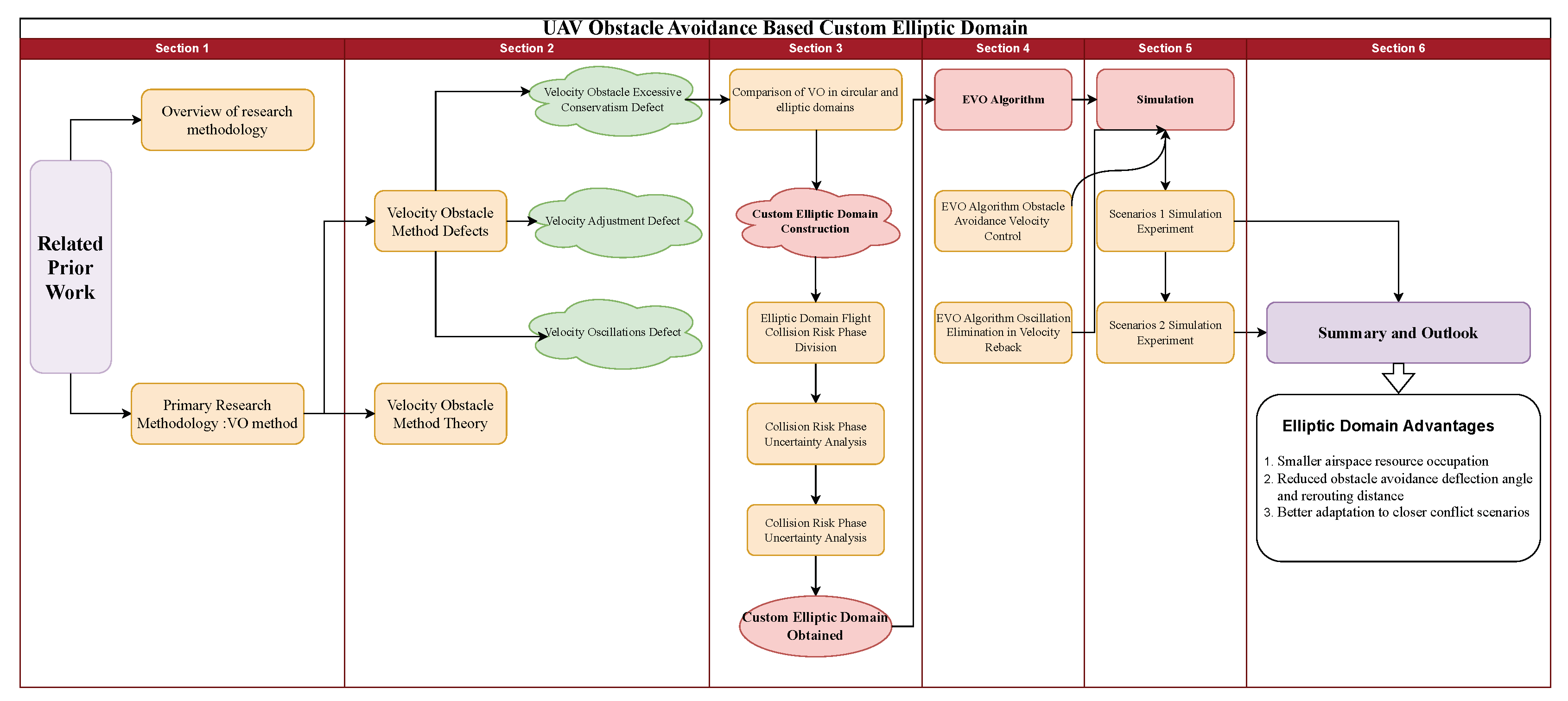
As unmanned aerial vehicles (UAVs) are widely used in various fields such as road traffic planning, military reconnaissance, agricultural production, and logistics distribution, the demand for low-altitude UAVs in segregated or integrated airspace will gradually increase in the foreseeable future. The operational safety of UAVs in low-altitude airspace and urban inter-traffic connections will be particularly important. A prominent issue in this regard is the collision avoidance problem of UAVs. There have been significant research achievements in addressing the collision avoidance problems of UAVs (or unmanned surface vessels, robots) in different research fields. The solutions can be categorized into global optimization control methods and local real-time avoidance methods.

The global optimal control method is based on the idea of mathematical optimization, and the required UAV navigation environment and flight state information is more complete, which can usually be planned to obtain a collision-free global navigation route under the specified constraints. Fu [1] utilized the additional flight distance of unmanned aerial vehicles as the maneuvering cost function. Initially, they computed the feasible solutions for initial collision avoidance using stochastic parallel gradient descent (SPGD) and then employed sequential quadratic programming (SQP) to determine the optimal collision avoidance heading. Sarim [2] proposed a combined solution based on A* mixed integer linear programming for the initial path planning of multiple unmanned aerial vehicles with individual task requirements and dynamic constraints. Sunberg [3] converted the multi-UAV conflict resolution problem into an approximate dynamic programming problem to solve. In addition, heuristic algorithms such as particle swarm optimization (PSO) and the genetic algorithm (GA) have considerable potential applications due to their efficient search capabilities in complex scenarios. Phung [4] effectively explored the configuration space of unmanned aerial vehicles by establishing corresponding relationships between particle positions and the UAV’s speed, turning angle, and climb/descent angles. They utilize PSO to find the optimal path that minimizes the cost function. Pehlivanoglu [5] integrated GA, Voronoi diagrams, and clustering methods, proposing an initial population enhancement approach to accelerate the convergence process, thereby obtaining feasible optimal paths in a short time. The starting point of the above global optimization control methods is based on the entire process of aircraft conflict, aiming to satisfy the optimization goal of minimizing a certain cost payment. However, they suffer from poor real-time performance and limited operability. These methods are difficult to apply when the complete global aircraft flight data are unknown and the conflict positions are uncertain. Moreover, the challenge of solving large-scale problems with slow convergence speeds persists.

On the other hand, local real-time path planning methods do not optimize the entire flight path of the aircraft but rather focus on conflict detection and avoidance. The main methods include artificial potential field (APF) and velocity obstacle (VO). APF has the advantage of a short response time and small problem-solving scale but often fails to produce a flight trajectory directed towards the target point. By setting virtual targets, this issue can be addressed, allowing for the correct navigation of the drone to avoid obstacles and reach the target point [6,7]. Pan [8] also introduced a rotational potential field to help the drone escape local minima and oscillation phenomena, facilitating the navigation of drone formations and clusters. The VO method, originally proposed by Paolo Fiorini [9], is a prominent obstacle avoidance strategy that converts the positional collision potential in the motion space of an agent into the velocity vector space [10]. This method delineated the entire set of velocities that could lead to a collision with an obstacle within a finite time as the ‘velocity obstacle space’ (VO space). By assigning the UAV a new linear velocity vector outside this defined set, the method ensured that the UAV can circumnavigate the obstacle within a permissible time frame, thereby eliminating collision risks. The method has excellent geometric intuition and does not require a complex modeling process. The 2D VO theoretical model simplified the UAV as a circle domain; this geometric central symmetry significantly eases the calculation of the ‘VO space’. However, this circle assumption uniformly scaled the conflict risk in all flight directions, potentially rendering conflict resolution schemes as overly conservative [10]. This could lead to operational failures in scenarios with high conflict numbers or dense UAV flights. For the same obstacle avoidance problem, there were also differences in whether or not to collide under circle protection domains with different radius scales, and if so, in the direction of the chosen resolution.

Current research on UAV obstacle avoidance using the VO method typically employs an empirical or artificially assigned fixed-radius circle protection domain [11,12,13,14,15]. Commonly, this radius is set by default as the UAV’s detection range; when another UAV enters this range, a potential collision is presumed to have occurred. This radius of this protection domain was not determined by the specific obstacle avoidance capabilities of the UAV, which compromises its scientific validity. Such an approach unnecessarily reduces the available free space—the area not occupied by the UAV’s flight path—potentially leading to suboptimal utilization of the navigable airspace.

From the perspective of minimizing the spatial size of the protection domain while ensuring sufficient safe space for UAV operation, substituting the circle domain with an elliptical domain is a practical option. This change not only maintains the smooth continuity of the boundary of the protection domain but also reflects the physical form of the intelligent agents more accurately. Circles tend to overestimate the necessary protection space for bodies that do not exhibit radial symmetry, while ellipses can more closely conform to the actual boundaries of the intelligent bodies. This adaptation was particularly beneficial in specific obstacle scenarios, such as navigating near walls, where circle domains may unnecessarily increase the detour distance [16,17]. Moreover, the geometric properties of elliptical domains offer broader applicability—circles are merely special cases of ellipses. Most agents, including ships and humanoid robots, do naturally conform to a elliptic boundary. Furthermore, the application of elliptical domains in the fields of pedestrian locomotion [18] and biomechanics [19] has demonstrated that ellipses provide a more accurate approximation of human movement.

In obstacle avoidance research utilizing the VO method, many researchers are aware of the drawbacks of circular domains but still compromise because of the simplicity of the computation. Still, several scholars had adopted an elliptical boundary domain. Lee [20] tackled the local obstacle avoidance problem for elliptical robots by approximating both the robots and obstacles with a minimum area boundary ellipse, implementing VO in two stages: acquiring a new linear velocity and correcting the angular velocity. Wang noted the substantial difference between longitudinal and transverse velocities in ground vehicle operations and designed an elliptical lattice boundary based on the vehicle’s travel direction, velocity, minimum safe distance, and lane width to model the motion of connected automated vehicle (CAV) clusters [21]. Furthermore, various studies [22,23,24] on unmanned surface vehicles (USVs) hved adopted elliptic domains. Liu and Bucknall [25] also suggested a circular shape for slow-moving obstacles and elliptical shapes for fast-moving obstacles. Additionally, elliptical boundary agents have been applied to research on obstacle avoidance using potential field theory [26] and limit cycle theory [27].

In contrast, the development of elliptic domains has not been exploited in the field of UAV obstacle avoidance. Similar to the conclusions in the literature [21,25], UAVs also characteristically exhibit a significantly higher longitudinal velocity compared to their transverse velocity. Current VO obstacle avoidance studies typically only establish a circle protection domain whose size substantially exceeds that of the individual UAV, leading to notable issues of spatial redundancy and unscientifically set initial values for the radius. We investigated the obstacle avoidance flight process of UAVs in head-on conflict scenarios and innovatively proposed a customized elliptical domain structure related to the separation distance and flight performance of the conflicting UAV pairs. We conducted a qualitative comparison of the velocity obstacles for circular and elliptical domains, validating the advantages of the elliptical domain in simulations that achieve the same safety distance requirements for obstacle avoidance.

1.2. Organization

The remainder of this paper is structured as follows: Section 2 reviews the basic principles and related defects of the VO method. In light of these defects, we articulate the main contributions of our work. In Section 3, we explore the feasibility of elliptical domains and propose designing an elliptic domain size linked to the UAVs’ flight state (velocity direction, velocity magnitude, angular velocity, and spatial distance), resulting in a custom elliptic domain. Section 4 introduces the elliptical velocity obstacles (EVO) method tailored for the boundaries of elliptic domains, establishing the elliptical absolute velocity obstacles (EAVO) as the core of our obstacle avoidance strategy. We also develop a velocity recovery rule to prevent one-sided velocity oscillations in Section 4. In Section 5, we validate our approach using MATLAB simulation experiments. Our results demonstrate that the EAVO’s resolution strategy addresses the over-conservative velocity and space wastage issues prevalent in circle domain VO applications, offering a smaller spatial footprint, a broader range of potential velocity directions, and robust resolution performance, particularly in flight scenarios with narrow separation distances. Finally, the results are discussed and summarized, and studies to improve the method are proposed in Section 6. The research process and architecture of this study are shown in Figure 1.

2. Review of Velocity Obstacle Method

2.1. Velocity Obstacle Method Theory

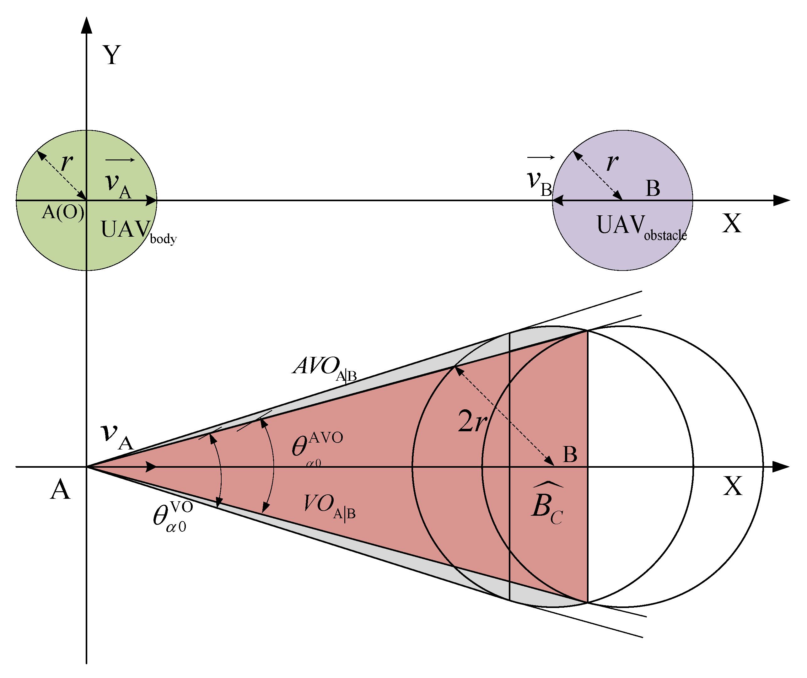
2.1.1. Minkowski Sum

The Minkowski sum serves as the mathematical foundation of VO theory and is integral to forming the velocity obstacle space. Essentially, a computational geometry operation, the Minkowski sum in Euclidean spaces is calculated by adding each vector from two non-empty sets, ‘A’ and ‘B’. Typically, this operation is defined as follows:

$$A\oplus B=\left\{a+b|a\in A,b\in B\right\}$$

(1)

where ⊕ is Minkowski sum notation.

Equation (1) delineates that for each vector in set ‘A’ and each vector in set ‘B’ a new vector in the Minkowski sum can be formed by their addition. This computation is straightforward for convex polygons. Non-convex challenges are often transformed into convex ones for resolution, lending the method broad applicability. In two dimensions, if ‘A’ and ‘B’ are polygons, their Minkowski sum results in a new polygon that encapsulates all possible combinations of their relative positions.

The Minkowski sum also provides a geometrically intuitive representation within the method. It is visualized as the area swept by set ‘A’ as it traces the perimeter of set ‘B’ combined with the area of set ‘B’ itself. If the elements of sets ‘A’ and ‘B’ within an algebraic system adhere to the properties of an Abelian group, the Minkowski sum also complies with the commutative law ($A\oplus B=B\oplus A$), reflecting the interchangeability of the summands. It is evident that the Minkowski sum is commutative within a two-dimensional real vector space. To clearly differentiate the research subjects in this paper, we define $A\oplus B$ to denote the Minkowski sum imposed by set ‘A’ on set ‘B’. This symbolization helps define the construction of the velocity obstacle space in the region where set ‘B’ is affected. For two methods on the computation of convex polygonal Minkowski sums, see Appendix A.1.

2.1.2. Velocity Obstacle Cone Construction

The velocity obstacle method was developed with a focus on circle robots and obstacles whose instantaneous states are measured or known. This approach allows for the simplification that disregards the computational discrepancies caused by the rotation of objects and their varying orientations [9]. For ease of description, this paper not only uses A and B to denote the two UAVs but also to represents the circle or elliptical protection domains in which A and B are located. The collision cone $C_{A,B}$ is defined in the literature [9] as the set of relative velocities that could lead to collisions between A and B. Superimposing $C_{A,B}$ onto the velocity of B defines the avoidance space in terms of B’s absolute velocity. This can be denoted as follows:

$$\left\{\begin{array}{cc}\hfill C_{A,B}& =\left\{v_{A,B}|{\lambda }_{A,B}\cap \widehat{\mathrm{B}}\ne \varnothing \right\}\hfill \\ \hfill VO& =C_{A,B}\oplus v_B\hfill \end{array}\right.$$

(2)

where $v_{A,B}$ is the velocity of A with respect to B, and ${\lambda }_{A,B}$ is the line on which vector $v_{A,B}$ lies. A ‘collapses’ to a point $\widehat{\mathrm{A}}$, and B ‘expands’ to $\widehat{\mathrm{B}}$, a circle region of twice the original radius. We prove this concisely in Appendix A.2. Equation (2) represents the region where relative velocity intersects with the velocity obstacle, forming a velocity obstacle cone. By superimposing the speed of Drone B, we can obtain the absolute velocity obstacle cone for Drone A.

The original definition of the velocity obstacle method involves adjusting the velocity of UAV-A outside the VO to avoid collisions. By integrating this classical VO definition and incorporating a time slice $\tau$, the VO and EVO models are summarized and redefined into three expressions in this paper:

$$\left\{\begin{array}{c}\widehat{B_C}=A\oplus B\hfill \\ V{O}_{A|B}^{\tau }=\left\{v_{A,B}|\exists t\in \left[0,\tau \right]::t{v}_{A,B}\cap \widehat{B_C}\ne \varnothing \right\}\hfill \\ AV{O}_{A|B}^{\tau }=V{O}_{A|B}^{\tau }\oplus v_B\hfill \end{array}\right.\left(circledomain\right)$$

(3)

$$\left\{\begin{array}{c}\widehat{B_E}=A\oplus B\hfill \\ EV{O}_{A|B}^{\tau }=\left\{v_{A,B}|\exists t\in \left[0,\tau \right]::t{v}_{A,B}\cap \widehat{B_E}\ne \varnothing \right\}\hfill \\ EAV{O}_{A|B}^{\tau }=EV{O}_{A|B}^{\tau }\oplus v_B\hfill \end{array}\right.\left(ellipticdomain\right)$$

(4)

For clarity of presentation, we made $V{O}_{A|B}^{\tau },EV{O}_{A|B}^{\tau }$ represent $C_{A,B}$ in the original definition of the velocity obstacle method. At each time interval $\tau$, the velocity obstacle cone for the drone can be obtained at each detection moment during the obstacle avoidance process, allowing for discrete conflict monitoring based on the calculated results.

The three variables above on the left side of Equations (3) and (4) are named the velocity obstacle set, the relative velocity obstacle cone, and the absolute velocity obstacle cone, respectively. The variable ‘t’ represents time. According to the definitions used in this paper, the VO for circle domains with equal radii at any location is illustrated in Figure 2. The elliptic domain Minkowski sums $\widehat{B_E}$ cannot be generated directly from the superposition of the geometric radius; thus, we require specially designed algorithms for implementation.

2.2. Velocity Obstacle Method Defects

2.2.1. Velocity Obstacle Excessive Conservatism Defect

The previous research related to the VO of the assumption of circle and elliptic domains has been briefly described in Section 1. Despite the computational benefits, we know the use of circles for multi-agent navigation results in many challenges. In many cases, a circle overestimates the actual profile of the robots that it represents [10]. In scenarios where the geometric appearance of agents closely resembles an ellipse, using an elliptical protection domain is a logical choice. The adoption of geometrical bodies that more closely resemble the appearance of the study subjects simplifies the obstacle avoidance modeling process. Essentially, this idea tends to ensure that the simulation results of abstract geometric bodies are more aligned with the actual movement of intelligent agents, eliminating redundant and unnecessary protection domains. From this perspective, assuming a circular radar range as the protective domain for UAVs is undeniably overly conservative. For a pair of UAVs in head-on conflict, if there is no interference, collisions would invariably occur in the direction of the velocity. Therefore, it is sensible to provide ample protection space in the direction of the velocity and reduce the protection space in unnecessary directions.

2.2.2. Velocity Adjustment Defect

The velocity obstacle method assumes that UAVs adjust their velocity states instantaneously upon detecting conflict risks, requiring highly sensitive sensors and efficient control algorithms for devising obstacle avoidance strategies [11]. If the length of time for velocity adjustment is considered, the VO space will be transformed into an area where the relative velocity obstacle cone sweeps through this length of time, necessitating greater velocity changes and occupying more space, which is disadvantageous for navigation in tight spaces. Moreover, the assumption that velocity changes instantaneously is not applicable when obstacle velocities are nonlinear, as the direction and magnitude of obstacle speeds can change at any moment, complicating the obstacle space dynamics. The discrete-time nonlinear velocity obstacle method (NLVO) [28,29,30,31] offers an effective solution for these challenges.

2.2.3. Velocity Oscillation Defects

Another notable problem is the oscillation of velocity selection. This issue arises when two conflicting entities simultaneously choose velocities for the next moment that are deemed collision-free. New velocities can lead to misjudgments about collision risks, prompting a return to original velocities. This cycle repeats, with each subsequent velocity adjustment reintroducing the potential for collisions. This phenomenon typically occurs due to a default preference for a higher-priority velocity direction $v_{prefer}$, often the initial velocity. As soon as a collision is detected or disappears, the velocity is approached toward $v_{prefer}$ immediately at the next moment.

To address this common problem in VO applications, Van Den Berg [32] proposed the reciprocal velocity obstacle (RVO) method, where the original VO is shifted by a specified time–displacement distance by translating it along $\left(v_A+v_B\right)/2$. By referring to the newly defined obstacle cone, one can effectively judge and mitigate collisions and oscillations among autonomous agents. This approach implies that both conflicting parties equally share the responsibility for collision avoidance. The RVO method has been extensively utilized in research on obstacle avoidance and safe navigation for dynamic agents [33,34,35]. Nonetheless, challenges persist due to disagreements and desynchronization over navigation preferences [36], potentially leading to ineffective collaboration and a reciprocal dance of avoidance [37]. To address this issue, Jamie [38] proposed the hybrid reciprocal velocity obstacle (HRVO) method, which modifies the passive avoidance approach in RVO by basing the future trajectory of robots on more than just a simple estimation of the current velocity [39].

2.3. Our Contributions

In response to the drawbacks identified in the VO methods outlined above, we have made specific improvements. For the issue of overly conservative circular domain structures, we aim to establish an elliptical domain that adequately protects UAVs while reducing the redundancy of the circular domain. Furthermore, to mitigate the adverse effects of sudden velocity shifts on obstacle avoidance decisions, we analyzed the UAV’s positional errors under tiny time deflection assumptions. By incorporating this positional uncertainty into the elliptical domain structure, we can continue to generate obstacle avoidance velocities through the absolute velocity obstacle cone (Section 3). Concurrently, due to the computational costs associated with precisely solving the Minkowski sum of the elliptical domain, we propose a discretized elliptical boundary accelerated algorithm using convex polygons (Section 4).

As for addressing velocity oscillations, RVO has already been widely adopted. This article is different from the above research on the fully autonomous obstacle avoidance mode of one or more agents. We provides a solution to the velocity oscillations of UAVs with motion priority. Unlike the previous assumption that both conflicting agents share responsibility for collision avoidance [32], this model designates only one UAV in the conflict as being responsible for adjusting its velocity to avoid potential obstacles, while the other UAV maximizes the usage of its original flight path, maintaining a steady course (Section 5). This approach could be particularly relevant in future urban logistics scenarios where, for example, delivery UAVs tasked with off-site deliveries may be given higher priority over UAVs returning for landing, reflecting typical head-on conflict characteristics. Additionally, the integration of UAVs actively avoiding manned aircrafts in fusion airspace is also a potential application scenario.

3. Custom Elliptic Domain Construction

In this part, we refine the original uniform circle protection domain structure with a fixed radius used in the VO method, replacing it with a custom elliptical domain structure that adapts to the UAV’s flight state. It is shown that a circular domain with a given radius may be redundant, and the actual elliptical domain based on the UAV’s flight conditions is much more accurate and still ensures that the UAV can avoid obstacles while satisfying the flight performance. To avoid the complexities present in initial studies, we continue to focus on the interaction between two UAVs flying in opposite directions, designated as A and B.

3.1. Comparison of VO in Circular and Elliptic Domains

Based on the review of the theoretical basis and fundamental principles of the velocity obstacle method, we can derive the following basic conclusions:

• The mathematical principle of the velocity obstacle space is the Minkowski sum of the boundary curves of two spatial objects. Geometrically, the Minkowski sum of two colliding entities represents the region swept by object A along the boundary of object B as it moves continuously for one revolution, combined with object B.
• When both objects are circles, their Minkowski sum is a circle with a radius equal to the sum of the radii of the two objects. For circles of the same size, their Minkowski sum is a circle with twice the radius.
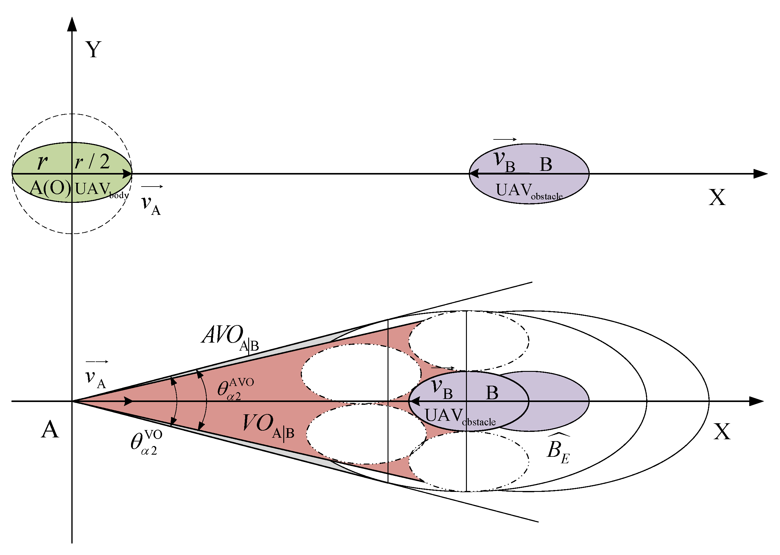
• Based on the proof that the Minkowski sum of two circles remains a circle, it can be anticipated that the precise calculation of the Minkowski sum and velocity obstacle cone for two elliptical objects will be more difficult. The reason for this is that in Equation (A1), the radius ‘r’ becomes the non-uniform semi-axis of the ellipse, making it challenging to simplify the computation of the maximum value. The distances from any point on ellipse A to the farthest point from the center of ellipse B obtained through iterative calculations will vary, indicating that the boundary of the Minkowski sum of two ellipses may not possess simple geometric characteristics. Therefore, further algorithmic solutions are required to address the velocity obstacle for elliptical boundaries.

3.1.1. Description of UAV Collision Stations

By approximating the obstacle boundary with the translation of the ellipse, a qualitative comparison of the velocity obstacle between circular and elliptic domains can be conducted. A and B are a pair of UAVs flying in opposite directions at the same altitude. If no avoidance measures are taken, they will collide at some point in the future. We set A’s spatial position at the coordinate origin, with the line connecting A and B along the horizontal axis (X-axis) and the vertical direction to the X-axis representing the Y-axis, thereby establishing a two-dimensional Cartesian coordinate system. Four types of protective domain combinations were constructed as comparative scenarios, denoted as ${\alpha }_0,{\alpha }_1,{\alpha }_2,{\alpha }_3$. The structural relationships and collision schematic diagrams for these four scenarios are illustrated in Figure 3, Figure 4, Figure 5 and Figure 6. Among these, the velocity obstacle spaces generated within the elliptical domains in stations ${\alpha }_2$ and ${\alpha }_3$ are approximate calculations, while the results in stations ${\alpha }_0$ and ${\alpha }_1$ are completely precise.

Station ${\alpha }_0$: Assuming the protective domain of the UAV is a circle of equal size, let A represent the obstacle-avoiding UAV and B represent the obstacle UAV. The velocity obstacle set between A and B forms a large circle with a radius of $2r$. By drawing a tangent line to this large circle from an external point at the origin, we obtain a conical region known as the relative velocity obstacle cone. By translating this relative velocity obstacle cone using the velocity vector, we derive the absolute velocity obstacle cone of A with respect to B. This cone represents the set of velocities that A must avoid in order to evade B.

Station ${\alpha }_1$: Keeping the state information of A and B unchanged in Station ${\alpha }_0$, we double the radius of B’s protective domain to obtain a velocity obstacle set represented by a circular area with a radius of $3r$ after the ‘expansion’.

Station ${\alpha }_2$: Assuming the UAV’s protective domain is an elliptic area, with A and B being isomorphic, the elliptic domain is contained within the initial circular domain. By geometrically describing the approximate velocity obstacles of both entities, we can simply translate UAV A’s elliptic domain several times until it is tangent to the boundary of B. We then envelop several tangential ellipses with a larger elliptic boundary, using this large ellipse to approximate the relative velocity obstacle set of A concerning B. Similarly, by approximating the tangent lines, we obtain the relative velocity obstacle cone, which, after translation, forms the absolute velocity obstacle cone.

The UAV’s protective domain is an elliptical area, with A and B being isomorphic. The elliptical domain encompasses the initial circular domain, with a short semi-axis of r and a long semi-axis of $1.5r$, while all other assumptions remain unchanged.

3.1.2. Comparison of UAV Collision Stations

• Comparison of station ${\alpha }_0$ and station ${\alpha }_1$: A and B both have circular protective domains. In the same collision scenario, the double protective domain of B in station ${\alpha }_1$ will cause a significantly larger velocity obstacle space compared to station ${\alpha }_0$. The target avoidance velocity obtained in station ${\alpha }_1$ will require a greater angular deviation. Therefore, a critical issue in applying the velocity obstacle principle to ensure collision-free operation for UAVs is determining the appropriate range of these protective domains. It is clear that avoidance decisions and outcomes are sensitive to the initial radius of this area. If the protective domain is too large, it compresses the available free space, leading to increased avoidance costs. Conversely, if the protective domain is too small, the performance requirements for the UAV during avoidance maneuvers increase, along with associated safety risks. Exploring a suitable and safe structure for the protective domain is a primary focus of this research.
• Comparison of station ${\alpha }_0$ and station ${\alpha }_2$: While maintaining a constant protective distance in the direction of the speed, the protective distance in the normal direction of the speed is reduced. Consequently, the absolute speed obstacle angle is also decreased. This indicates that constructing a collision-free zone in the shape of an elliptical domain with a short axis can not only ensure safe obstacle avoidance but also minimize the utilization of airspace resources.
• Comparison of station ${\alpha }_0$ and station ${\alpha }_3$: In station ${\alpha }_3$, the elliptical domain completely encompasses the circular domain from station ${\alpha }_0$, resulting in a velocity obstacle space that also covers the velocity obstacle space obtained from the circular domain. In station ${\alpha }_3$, the protective distance in the normal direction of the speed remains at r, while the protective distance in the velocity direction increases by $0.5r$. As a result, the velocity obstacle angle also increases accordingly. This demonstrates that both axes of the ellipse have an impact on the calculated results of the velocity obstacle space.

Based on the comparison above, it is evident that the elliptical structure in station ${\alpha }_2$, while maintaining the original protective space in the direction of speed, has corrected the overly conservative circular domain by reducing the size in the normal direction of speed. If there are established safety distance requirements, this dimension should be fixed along the major axis of the ellipse. For the same drone collision event, the avoidance velocity sets calculated from the different protective domain structures in station ${\alpha }_0,{\alpha }_1,{\alpha }_2,{\alpha }_3$ vary accordingly. Therefore, our objective is to design an elliptical protection domain that ensures the safe flight of the drone while providing a certain degree of redundancy. To the greatest extent possible, we provide a larger protective domain space in the collision direction while minimizing unnecessary dimensions in non-collision directions. Theoretically, this approach can offer the drone a more diverse selection of obstacle avoidance velocity options.

3.2. Elliptic Domain Flight Collision Risk Phase Division

A Cartesian coordinate system was established with the initial position of UAV-A as the origin. The size of the elliptical protection domain is related to the UAV’s flight state, ensuring that the geometrical structure can still be relieved, even under the least ideal conditions conditions. The model is configured as follows:

In this study, we configure the UAV to update the detection of its surroundings every $\tau$ seconds. Upon detecting an obstacle, the UAV will initiate an avoidance maneuver. It is important to note that throughout this research, adjusting the direction of velocity has been consistently used as the primary means of obstacle avoidance. This approach aligns with the ideal collision resolution under the VO principle. An adjustment that alters only the magnitude of the velocity, without changing its direction, may put off the conflict into a subsequent time period, especially when UAV-B is in linear motion. After detecting an obstacle and identifying a new velocity target orientation, the UAV most at risk of collision has approximately $\tau$ seconds—excluding the time spent computing the obstacle cone and selecting a new velocity—to reorient towards the target. Consequently, the maximum possible deflection achievable by the UAV within $\tau$ seconds sets the minimum threshold necessary for collision avoidance.

Assuming that the maximum deflection angle of the UAV per one second is $\phi$ (rad), the minimum threshold on the deflection that can be made within $\tau$ is ${\phi }_{inf}=\tau \phi$. In scenarios where UAVs encounter head-on conflicts, if both UAVs simultaneously maneuver to the right with the same constant angular velocity towards a predetermined target direction, the collision can be avoided if their protective domains do not overlap. The entire obstacle avoidance process is divided into two phases: ‘Phase 1: Conflict risk phase’ and ‘Phase 2: Conflict risk elimination phase’. Phase 1 is a deflection flight process, while Phase 2 is a directional process. The active avoidance maneuvers occur during Phase 1. A schematic diagram illustrating this is provided below, where $p_{link}$ is the two-phase transition node. UAV-A and UAV-B have equal elliptic domains.

In the second phase, where the velocities of the two UAVs are parallel but not collinear, overlaps in the protective domains can occur if the steering adjustments from the first phase are inadequate. This overlap might stem from higher longitudinal velocities or smaller intervals between obstacle detections. As illustrated in Figure 7, when both UAVs employ the same avoidance strategy, their directions align at any given moment, and the major and minor axes of their elliptical domains remain parallel, with UAV-B consistently positioned above UAV-A. Therefore, potential overlaps during Phase 1 could manifest as one of three types: frontside, backside, or topside intrusions, as depicted in Figure 8.

When analyzing the three relative positional relationships, collisions can be averted in each scenario as long as the distance between the centers of the two ellipses, when projected along the direction of the minor axis, remains greater than the length of the minor axis (2b) throughout Phase 1.

3.3. Collision Risk Phase Uncertainty Analysis

3.3.1. Collision Risk Phase Uncertainty Assumptions

At the critical moment when a UAV anticipates a collision risk using the VO principle, the essence of obstacle avoidance lies in adjusting the velocity direction to fall outside the VO. According to the VO method, the velocity is presumed constant within the interval $\tau$, changing only at the moment a decision is made to avoid an obstacle. This necessitates frequent sensor refreshes [11], which can lead to discrepancies between the actual flight position and the VO theoretical one. This means that at every moment, the actual position of the drone deviates from the estimated position. Such endpoint location uncertainty may continuously accumulate, potentially impacting the design of the elliptical protection domain size. Therefore, we categorize the deflection process into three assumptions and discuss them below.

• Assumption 1: Segmented Multiple Tiny Deflections
  Assume that the drone’s directional adjustments are linearly varied over each time interval. Segmented, multiple, tiny deflections provide a smoother representation of the actual flight process. This method suggests that the angular velocity during the deflection process remains constant throughout each tiny time interval. The UAV produces consistent angles of deflection over identical, short periods, with the cumulative deflection angle increasing incrementally. Simply put, Assumption 1 is a gradual deflection process, which corresponds to the blue line in Figure 9.
• Assumption 2: Deflection Along the Average Deflection Angle
  Deflection along the average deflection angle means that the UAV is oriented towards the target with the average angle $\overline{\theta }$ of Assumption 1. The endpoint of the blue line in Figure 9 represents the flight position obtained from Assumption 1, and the heading angle towards this endpoint from the initial position is denoted as $\overline{\theta }$. The UAV will fly along this direction instantly when the risk of collision is detected, which corresponds to the red dashed line in the middle of Figure 9.
• Assumption 3: Deflected Along the Target Deflection Angle
  This assumption is the default assumption of the VO method. It specifies that upon detecting a collision threat, the UAV will immediately navigate in the direction of a velocity selected outside the AVO, which is named as the target deflection angle. In simple terms, the drone initially adjusts its heading to fly along the final flight angle defined by Assumption 1, which corresponds to the red dashed line at the bottom of Figure 9.
  The flight process for a given time interval $\tau$ under the three assumptions is demonstrated in Figure 9. It is obvious that the flight endpoints are different across the three different assumptions.

3.3.2. Collision Risk Phase Error Expression Derivation

The line velocity of the UAV deflection process is constant in magnitude. Only the direction of the velocity changes, discretizing the UAV deflection process into n linear deflection microelements. The time step within each microelement is $\tau /n$, and the displacement distance is $v\tau /n$. Thus, one UAV will produce a total displacement during the time interval $\tau$:

$$s=\Sigma {\displaystyle \frac{v\tau }{n}}+\cdots +{\displaystyle \frac{v\tau }{n}}=v\tau$$

(5)

The UAV can be deflected by $\phi \tau /2$ at a maximum angular velocity during $\tau$. The UAV deflection angles form an arithmetic progression with time microelements. The formula for the general term of the arithmetic series is $a_n\left(n=1,2,\cdots ,n\right)$, the common difference is $d\theta =\phi \tau /2n$, and the sum of the first n terms is $S_n$, where n denotes the number of microelements. Then, the construction shown in Figure 9 will form an n + 1 sided polygon. The average deflection angle can be expressed as follows:

$$\overline{\theta }=a_1+{\displaystyle \frac{\left(n+1-2\right)\pi -\left(n-1\right)\left(\pi -d\theta \right)}{2}}=a_1+{\displaystyle \frac{\left(n-1\right)d\theta }{2}}$$

(6)

Since the deflection from the horizontal is 0 degrees, there is essentially $a_1=d\theta$. Thus, the above equation can be simplified to:

$$\overline{\theta }={\displaystyle \frac{n+1}{2}}d\theta$$

(7)

which is exactly the mean of the sum of the n terms of the angular equidistant series:

$$\overline{S_n}={\displaystyle \frac{S_n}{n}}={\displaystyle \frac{n\left[a_1+a_1+\left(n-1\right)d\theta \right]}{2n}}=a_1+{\displaystyle \frac{(n-1)d\theta }{2}}=\overline{\theta }$$

(8)

Therefore, $\overline{\theta }={\displaystyle \frac{\mathrm{n}+1}{2}}·{\displaystyle \frac{\phi \tau }{2n}}={\displaystyle \frac{n+1}{4n}}\phi \tau \Rightarrow {lim}_{n\to \infty }\overline{\theta }={\displaystyle \frac{\phi \tau }{4}}$

Next, it is proved that the displacement endpoints obtained under Assumptions 1 and 2 have small errors. Decompose the velocity in each microelement in both the horizontal and vertical directions and accumulate these to obtain the displacement distance in both directions in $\tau$:

$$\left\{\begin{array}{c}\mathit{\Delta }x=v\underset{n\to \infty }{lim}\sum _{i=1}^{n}cos({\displaystyle \frac{\phi \tau }{2}}·{\displaystyle \frac{i}{n}})·{\displaystyle \frac{\tau }{n}}=v\tau \underset{0}{\overset{1}{\int }}cos({\displaystyle \frac{\phi \tau }{2}}·x)dx={\displaystyle \frac{2v}{\phi }}sin{\displaystyle \frac{\phi \tau }{2}}\hfill \\ \mathit{\Delta }y=v\underset{n\to \infty }{lim}\sum _{i=1}^{n}sin({\displaystyle \frac{\phi \tau }{2}}·{\displaystyle \frac{i}{n}})·{\displaystyle \frac{\tau }{n}}=v\tau \underset{0}{\overset{1}{\int }}sin({\displaystyle \frac{\phi \tau }{2}}·y)dy={\displaystyle \frac{2v}{\phi }}\left(1-cos{\displaystyle \frac{\phi \tau }{2}}\right)\hfill \end{array}\right.$$

(9)

Then, generate a joint displacement: $s_1=\sqrt{\mathit{\Delta }{x}^2+\mathit{\Delta }{y}^2}={\displaystyle \frac{2v}{\phi }}\sqrt{2\left(1-cos{\displaystyle \frac{\phi \tau }{2}}\right)}$

For UAV-A, the coordinates of the end point of the flight by $\overline{\theta }$ are $(\mathit{\Delta }{x}^{\prime },\mathit{\Delta }{y}^{\prime })$:

$$\left\{\begin{array}{c}\mathit{\Delta }{x}^{\prime }=v\tau cos{\displaystyle \frac{\phi \tau }{4}}\hfill \\ \mathit{\Delta }{y}^{\prime }=v\tau sin{\displaystyle \frac{\phi \tau }{4}}\hfill \end{array}\right.$$

(10)

Then, generate a joint displacement: $s_2=\sqrt{{\left(\mathit{\Delta }{x}^{\prime }\right)}^2+{\left(\mathit{\Delta }{y}^{\prime }\right)}^2}=\tau v$

Align the displacements x and y along the $\overline{\theta }$. The displacement deviation $\mathit{\Delta }s$ can be expressed as a function of the UAV flight speed v, deflection avoidance time interval $\tau$, and deflection angle per unit time $\phi$. $\mathit{\Delta }s$ is defined as follows:

$$\mathit{\Delta }s\left(v,\phi ,\tau \right)=\left|s_1-s_2\right|=\left|{\displaystyle \frac{2}{\phi }}\sqrt{2\left(1-cos{\displaystyle \frac{\phi \tau }{2}}\right)}-\tau \right|·v$$

(11)

The mean value of the displacement deviation is defined as follows:

$$\mathit{\Delta }{s}^{\prime }={\displaystyle \frac{1}{n}}\sum _{i=1}^{n}v\left|{\displaystyle \frac{2}{{\phi }_i}}\sqrt{2\left(1-cos{\displaystyle \frac{{\phi }_i·dt}{2}}\right)}-dt\right|\left({\phi }_i={\displaystyle \frac{\pi }{3}},{\displaystyle \frac{\pi }{3}}+d\theta ,\cdots ,2\pi \right)$$

(12)

If the UAV is flying in the direction of the target from the beginning, there is also a distance difference $d_e$ between the endpoints of the displacements in Assumptions 2 and 3. We used the law of cosines in the red isosceles triangle in Figure 9 and obtained the following:

$$d_e\left(v,\phi ,\tau \right)=v\tau \sqrt{2\left(1-cos{\displaystyle \frac{\phi \tau }{4}}\right)}$$

(13)

3.3.3. Collision Risk Phase Error Analysis

When the UAV detection time scale is small, the UAV flight endpoint error $\mathit{\Delta }s$ about Assumptions 1 and 2 is small compared to the actual displacement scale, while the error $d_e$ about Assumptions 2 and 3 is much larger. Based on the expressions derived in Section 3.3.2 for $\mathit{\Delta }s$ and $d_e$, we plot the changes in their associated variables in Figure 10.

Figure 10a shows the variation in the function $\mathit{\Delta }s$ on $\left[0,2\pi \right]$. Figure 10b shows the projections of the two variables $\phi ,\tau$ on their corresponding axis planes, respectively. It can still be observed qualitatively without exact partial derivatives that the $\mathit{\Delta }s$ in a certain range around ‘0’ are low (Figure 10a). This indicates that the value of error $\mathit{\Delta }s$ is not significant when both $\phi$ and $\tau$ are small. Fixing one of the variables, taking several discrete values for the other variable, and changing their errors, we can see that all four curves are increasing (Figure 10c). This indicates that the partial derivative of the other variable is positive at its corresponding value. The purple and red curves grow slowly (corresponding to $\tau$ fixed), while the yellow and green curves grow fast (corresponding to $\phi$ fixed), so that time $\tau$ has a more pronounced effect on $\mathit{\Delta }s$ than the deflection angle $\phi$. This reveals that we prioritize the control shortening time. The error distance $\mathit{\Delta }s$ about Assumptions 1 and 2 will be lower.

By analyzing the functional relationship for $d_e$ over the same range of independent variables (see Figure 10d–f), we can obtain similar conclusions to $\mathit{\Delta }s$, except that most of the same independent variables $\phi ,\tau$ correspond to $d_e$ greater than $\mathit{\Delta }s$ (see Figure 10g–i). Hence, under Assumption 3 of the VO method, the position UAV-A reaches after executing the redirection maneuver may not align with its actual position, potentially encroaching into the VO space occupied by UAV-B. Our discussion of this part of the error is similar to the starting point of the NLVO [28,29,30,31].

In this paper, we address the fact that our UAV’s protection domain is neither pre-determined nor fixed. Consequently, the uncertainty error introduced by this linear assumption can be incorporated into the design of the protection domain. Equivalently, this displacement deviation is added to the original protection domain space so that the we can continue to adjust the UAV under Assumption 3 [11], simplifying the calculations and skipping the complex flight details of Assumption 1.

3.4. Elliptic Domain Size Construction Considering Uncertainty Errors

In Phase 1, as established in this paper, the average displacement deflection angle consistently remains smaller than the target deflection angle. Thus, under Assumption 3, the distance between the endpoints of UAVs A and B along the minor axis direction is invariably greater than that observed under Assumption 2. The minor axis defined under Assumption 3 contains the length of the error $d_e$. Upon analyzing the geometric logic, we conclude the following:

$$\left\{\begin{array}{c}{d}_b^i=d_{v\tau }^i·sin{\theta }_b^i\approx d_{\overline{\theta }}^i·sin{\theta }_b^i+2d_e\hfill \\ d_{v\tau }^i=\sqrt{{\left(y_{\mathrm{B}}^{{\tau }_i}-y_{\mathrm{A}}^{{\tau }_i}\right)}^2+{\left(x_{\mathrm{B}}^{{\tau }_i}-x_{\mathrm{A}}^{{\tau }_i}\right)}^2}\hfill \\ {\theta }_b^i={\beta }_{\tau }^i+{\displaystyle \frac{\phi \tau }{2}}·i-{\displaystyle \frac{\pi }{2}}\hfill \\ {\beta }_{\tau }^i=\mathrm{arc}tan\left({\displaystyle \frac{y_{\mathrm{B}}^{{\tau }_i}-y_{\mathrm{A}}^{{\tau }_i}}{x_{\mathrm{B}}^{{\tau }_i}-x_{\mathrm{A}}^{{\tau }_i}}}\right)\hfill \end{array}\right.$$

(14)

In the above equation, $d_b^i$ denotes the projected distance between the two ellipses in the direction of the minor axis at the moment ${\tau }_i$; $d_{v\tau }^i$, $d_{\overline{\theta }}^i$ denote the distance between the endpoints of the two UAV displacements under Assumptions 2 and 3 at each time step $\tau$, respectively; ${\beta }_{\tau }^i$ indicates the inclination of the terminal line under Assumption 3; ${\beta }_{\tau }^i$ indicates the angle between the displacement endpoint line and the direction of the normal velocity under Assumption 3. Since it has been proved in the previous section that $\mathit{\Delta }s$ is obviously smaller than $d_e$, ignoring $\mathit{\Delta }s$, the above equation is approximately equal.

If UAVs A and B are deflected to avoid obstacles at the initial moment under Assumption 3, the spatial position at the end of each time ${\tau }_i$ can be expressed as follows:

$$\begin{array}{c}\hfill \left\{\begin{array}{c}{x}_{\mathrm{A}}^{{\tau }_i}=x_{\mathrm{A}}^{{\tau }_0}+\sum _{i=1}^{n}v\tau ·cos\left({\displaystyle \frac{\phi \tau }{2}}·i\right)\hfill \\ y_{\mathrm{A}}^{{\tau }_i}=y_{\mathrm{A}}^{{\tau }_0}-\sum _{i=1}^{n}v\tau ·sin\left({\displaystyle \frac{\phi \tau }{2}}·i\right)\hfill \end{array}\right.\&\left\{\begin{array}{c}{x}_{\mathrm{B}}^{{\tau }_i}=x_{\mathrm{B}}^{{\tau }_0}-\sum _{i=1}^{n}v\tau ·cos\left({\displaystyle \frac{\phi \tau }{2}}·i\right)\hfill \\ y_{\mathrm{B}}^{{\tau }_i}=y_{\mathrm{B}}^{{\tau }_0}+\sum _{i=1}^{n}v\tau ·sin\left({\displaystyle \frac{\phi \tau }{2}}·i\right)\hfill \end{array}\right.\left(i\in N^{+}\right)\end{array}$$

(15)

To ensure that the UAV can effectively avoid collisions upon detecting a risk during Phase 1, within the constraints of its physical capabilities, the value of the length of the minor semi-axis of the ellipse (2b) must not exceed the minimum separation distance. We define this minimum value as the distance projection along the minor axis direction before the velocities of UAVs A and B are deflected to $\pi /2$. This is recorded as follows:

$$b_{min}^{\tau }=min\{d_b^i/2\}\left(i\in \lfloor {\displaystyle \frac{\pi }{2\phi \tau }}\rfloor \&i\in N^{+}\right)$$

(16)

Based on this, we anticipate that the lateral distance will also be sufficiently large to minimize the possibility of the collision scenarios depicted in Figure 8. Consequently, within each time step $\tau$, we have the following:

$$l_{v\tau }^i=\left(x_{\mathrm{B}}^{{\tau }_i}-x_{\mathrm{A}}^{{\tau }_i}\right)·cos\left({\displaystyle \frac{\phi \tau }{2}}·i\right)>0$$

(17)

Similarly,

$$a_{min}^{\tau }=min\{l_{v\tau }^i\}/2\left(i\in \lfloor {\displaystyle \frac{\pi }{2\phi \tau }}\rfloor \&i\in N^{+}\right)$$

(18)

Since A and B are generally asynchronous in reaching the minimum value, the equation $a_{min}^{\tau }>b_{min}^{\tau }$ does not necessarily hold. To avoid ambiguity, when $a_{min}^{\tau }<b_{min}^{\tau }$, we assign $a_{min}^{\tau }=1.5b_{min}^{\tau }$. In summary, the custom elliptic domain structure is given by the following constraints:

$$a_{min}^{\tau }>b_{min}^{\tau }:\left\{\begin{array}{cc}\hfill a_{min}^{\tau }& ={\displaystyle \frac{min\left\{l_{v\tau }^i\right\}}{2}}\hfill \\ \hfill b_{min}^{\tau }& ={\displaystyle \frac{min\left\{d_b^i\right\}}{2}}\hfill \end{array}\right.\left(i\in N^{+}\right)$$

(19)

$$a_{min}^{\tau }\le b_{min}^{\tau }:\left\{\begin{array}{cc}\hfill a_{min}^{\tau }& =1.5b_{min}^{\tau }\hfill \\ \hfill b_{min}^{\tau }& ={\displaystyle \frac{min\left\{d_b^i\right\}}{2}}\hfill \end{array}\left(i\in N^{+}\right)\right.$$

(20)

For a given velocity–position state, the values calculated above represent the elliptical domain sizes for the pair of reversed conflict UAVs, which are simplified as follows:

$$a=a_{min}^{\tau };b=b_{min}^{\tau }$$

(21)

The elliptic domain structure we constructed maps the ellipse’s major and minor semi-axes to the UAV speed, velocity direction, angular velocity performance, hostile UAV spacing distance, and UAV detection frequency. It has adaptability associated with the real-time status of the UAV. In Phase 1, if equation $d_b^i<2b$ is satisfied, they will intrude on each other at a certain moment; otherwise, they will never intrude. The projected distance in the minor-axis direction reflects the closest distance between the two in subsequent flights in the non-intrusive state and reflects the extent of mutual invasion between the two in the intrusive state.

4. EVO Algorithm-Based Custom Elliptic Domains

As elliptic domains no longer have the simplicity of calculating the VO space compared to the circle domains, the exact calculation of the Minkowski sum for the elliptic domains in which A and B are located involves either calculating the boundary convolution curves [40,41,42] or employing the close-form implicit equations [43] with more expensive computational costs. The computation of the tangent line at a point outside the non-circle domain will also become complicated. Lee and Beom H. [20] have accurately derived and computed the VO space and obstacle cones for the minimum area boundary ellipse approximation of obstacles with a high degree of complexity. The conservative linear computational method proposed by Best [10] is more efficient and has been validated under multi-obstacle experimental conditions. In addition to applying the VO method for obstacle avoidance in elliptical agents, Boolean operations on elliptical boundaries have also been utilized to address conflict scenarios in multi-ship encounters [31,44]. In this section, we approximate the boundary of the elliptical domain as a convex polygon, allowing for rapid computation of the VO space. The tangents of this space are efficiently estimated, too.

4.1. EVO Algorithm Preparations

This part discretizes the elliptic boundary in any axial direction to form a convex polygonal structure. According to the obtained custom elliptic domain size, the standard elliptic equation located at the coordinate origin is as follows:

$${\displaystyle \frac{x^2}{a^2}}+{\displaystyle \frac{y^2}{b^2}}=1$$

(22)

We take the center of the ellipse where UAV-A is located as the coordinate origin and the major and minor semi-axes as the direction of the X- and Y-axes coordinate system. Without a loss of generality, any axial UAV-B ellipse exists in this coordinate system with inclination angle $o_{\mathrm{B}}$ and center spacing distance $d_{\mathrm{AB}}$.

We discretize the boundary of the ellipse on which UAV-A is located by taking the ${\theta }_m$ angle. As a result, there will be $2\pi /{\theta }_m$ discrete points. Elliptic protected domains are transformed into convex polygons. Each discrete coordinate point can be represented as follows:

$$\left\{\begin{array}{cc}\hfill x_A^i& =acos{\theta }_i=acosi\ast {\theta }_m(i=1,\cdots ,2\pi /{\theta }_m)\hfill \\ \hfill y_A^i& =bsin{\theta }_i=bsini\ast {\theta }_m(i=1,\cdots ,2\pi /{\theta }_m)\hfill \end{array}\right.$$

(23)

where ${\theta }_i$ is the angle corresponding to every interval ${\theta }_m$, with 0 degrees in the positive direction of the x-axis and a positive counterclockwise rotation. With UAV-A as a reference, the discretized boundary points of B at any position and axial direction in this coordinate system are equivalent to two transformations of the boundary discretization points sought by A. Rotation transformation first and then translation transformation is equivalent to translation transformation first and then rotation transformation. If we rotate first using the clockwise rotation matrix Turn, the mapping is applied accordingly.

$$Turn=\left[\begin{array}{cc}cos{o}_{\mathrm{B}}& -sin{o}_{\mathrm{B}}\\ sin{o}_{\mathrm{B}}& cos{o}_{\mathrm{B}}\end{array}\right]$$

(24)

$$\left\{\begin{array}{cc}\hfill x_{B1}^i& =acosi\ast \overline{\theta }·Turn(i=1,\cdots ,2\pi /{\theta }_m)\hfill \\ \hfill y_{B1}^i& =bsini\ast \overline{\theta }·Turn(i=1,\cdots ,2\pi /{\theta }_m)\hfill \end{array}\right.$$

(25)

where $o_{\mathrm{B}}$ is the angle of rotation of B with reference to the direction of the major axis of A. After the rotation is completed, the coordinate points are translated to the location of B to obtain the discrete boundary points of B in the coordinate system:

$$\left\{\begin{array}{c}{x}_{B2}^i=x_B=x_{B1}^i+d_{AB}cos{o}_{\mathrm{B}}\hfill \\ y_{B2}^i=y_B=y_{B1}^i+d_{AB}sin{o}_{\mathrm{B}}\hfill \end{array}\right.$$

(26)

At this point, we have discretized the two elliptical protection domains corresponding to UAVs A and B into convex polygons and established coordinate correspondences for each node. Therefore, we obtain a set of discrete points on the boundaries of the elliptical domains of A and B:

$$\left\{\begin{array}{cc}\hfill Boundar{y}_A& =\left\{x_A^i,y_A^i\right\}\hfill \\ \hfill Boundar{y}_B& =\left\{x_{B2}^i,y_{B2}^i\right\}\hfill \end{array}\right.(i=1,\cdots ,2\pi /{\theta }_m)$$

(27)

4.2. EVO Algorithm Steps

Taking UAV-A as the subject of obstacle avoidance and evaluating the EAVO imposed on UAV-B, the following algorithm steps are executed:

• Step 1: Computation of Minkowski sum and convex hull boundary points

We considered the discrete convex polygons of UAVs A and B. The Minkowski sum, imposed by A on B, is calculated. Using Method 1 as described in Appendix A.1 of this paper, we employ the convex polygon convex hull algorithm to derive the convex boundary from the results of the discrete point summation:

$${\Omega }_{A\oplus B}=convhull\left\{Boundar{y}_A+Boundar{y}_B\right\}$$

(28)

We can obtain the convex hull structure by extracting the boundary point index. The 2D convex hull boundary is EVO space ($\widehat{B_E}$). This is the set of velocities we need to satisfy disjointness for obstacle avoidance. The discrete points on the convex hull boundary are marked as $Boundar{y}_{\widehat{B}}=\left\{p_i,i=\left(1,\cdots ,n\right)\right\}$, and it may be an elliptical-like structure.

• Step 2: Finding the approximate EVO space tangent line

Since the convex packet boundary is not smooth, the left and right derivatives of each discrete boundary point are not equal to each other. If it is not differentiable, the slope does not exist. Owing to the abundance of discrete boundary nodes and the small intervals between them, we efficiently utilize data from the convex hull algorithm by approximating the slope at any point within the discrete boundary set by using the slope of the line connecting the adjacent front and back nodes:

$$k_i={\displaystyle \frac{\mathit{\Delta }{y}_i}{\mathit{\Delta }{x}_i}}={\displaystyle \frac{y_{i+1}-y_{i-1}}{x_{i+1}-x_{i-1}}}$$

(29)

Then, we look for a point (where A is located) outside the convex hull tangent to it. We do this to find any point on the convex hull and the point where the slope of the line connecting A is consistent with $k_i$. We connect the boundary discrete points with position A, where the linear direction function is expressed in the slope as follows:

$$k_i^{\prime }={\displaystyle \frac{y_A-y_i}{x_A-x_i}}$$

(30)

The absolute errors of these slopes can be found for a series of discrete points:

$${\epsilon }_i=\left|k_i-k_i^{\prime }\right|\times 100\%$$

(31)

• Step 3: Return EVO space tangent points

Because more than one discrete point is close to the true tangent points within the error allowance, there is a risk of double-counting the tangent points. Therefore, the minimum and maximum slope values within this error range (${\epsilon }_{\mathrm{agree}}$) should be considered as the two approximate tangent points of the convex hull at that moment:

$$\left\{\begin{array}{c}{p}_{con}^1=\arg max\left(\mathrm{arc}tan{k}_i^{\prime }\right)=\left(x_{con}^1,y_{con}^1\right)\hfill \\ p_{con}^2=\arg min\left(\mathrm{arc}tan{k}_i^{\prime }\right)=\left(x_{con}^2,y_{con}^2\right)\hfill \end{array}\right.foreach{\epsilon }_i<{\epsilon }_{\mathrm{agree}}$$

(32)

where $p_{con}^1$ and $p_{con}^2$ are the two tangent points we computed.

The denser the discrete points, the smaller the error. Accordingly, ${\epsilon }_{\mathrm{agree}}$ can be set smaller. The approximation of the tangent line is closer to the true value, but the calculation becomes more time-consuming as a result.

• Step 4: Computation of EAVO

Translate all convex packet boundary points along $\overrightarrow{v_B}$ in $\tau$. The set of convex packet boundary points after translation is $Boundar{y}_{\widehat{B}}\oplus \overrightarrow{v_B}·\tau$. The position of the tangent points after translation is $p_{con}^1=(x_{con}^1,y_{con}^1)\oplus \overrightarrow{v_B}·\tau ,p_{con}^2=(x_{con}^2,y_{con}^2)\oplus \overrightarrow{v_B}·\tau$. We connect the translational tangent points $p_{con}^1$ and $p_{con}^2$ to the UAV-A coordinates to construct EAVO at a given moment in time: $EAV{O}_{A|B}^{\tau }=\left\{v|v\notin EV{O}_{A|B}^{\tau }\oplus v_B\right\}$.

4.3. EVO Algorithm Obstacle Avoidance Velocity Control

After determining the custom elliptic domain for the UAV, it is essential to establish a control scheme to adjust the velocity for obstacle avoidance. Additionally, we must address potential velocity oscillations that could arise during this process to prevent the UAV from entering a repetitive loop of obstacle avoidance maneuvers and course corrections. To streamline the process and minimize the time and complexity involved, this paper fixes the major and minor semi-axes under the initial ${\tau }_0$ computation as the ellipse size based on the analysis and discussion in Section 3. This eliminates the need for recalculating the ellipse size with each obstacle encounter.

We utilize the EAVO as the basis for obstacle avoidance. UAV-B has a higher navigational priority compared to A. We adjust only the direction of UAV-A’s velocity while keeping UAV-B’s heading unchanged. The EAVO for UAV-A is recalculated at the end of each time step ${\tau }_i$. If UAV-A’s velocity falls within the EAVO at point ${\tau }_{i-1}$, the heading of UAV-A is then adjusted accordingly. It is worth noting that we cannot always regard the boundary velocity of the cone as the adjusted orientation because of the limitations of UAV physical deflection capabilities. Additionally, the accuracy of the tangent line determination is influenced by the number of discrete boundary points, introducing some discrepancies between the actual position and the results of the approximation algorithm. To ensure adequate safety, in scenarios where only a minor deflection is necessary for obstacle avoidance, we deflect A into $\left[\phi \tau /2,\phi \tau \right]$. Therefore, there are three situations:

$$\stackrel{{\tau }_{i+1}}{new}=\left\{\begin{array}{c}\left\{\begin{array}{c}{o}_A^{{\tau }_i}-\phi \tau /2,o_A^{{\tau }_i}\in EAV{O}_{{\tau }_i}\&0<\left|o_{EAVO}^{{\tau }_i}-o_A^{{\tau }_i}\right|\le \phi \tau /2\Rightarrow \mathrm{Collision}\hfill \\ -\left|o_{EAVO}^{{\tau }_i}\right|,o_A^{{\tau }_i}\in EAV{O}_{{\tau }_i}\&\phi \tau /2<\left|o_{EAVO}^{{\tau }_i}-o_A^{{\tau }_i}\right|\le \phi \tau \Rightarrow \mathrm{Collision}\hfill \end{array}\right.\hfill \\ \left\{o_A^{{\tau }_i}-\phi \tau ,o_A^{{\tau }_i}\in EAV{O}_{{\tau }_i}\&\left|o_{EAVO}^{{\tau }_i}\right|>\phi \tau \Rightarrow \mathrm{Collision}\right.\hfill \\ \left\{o_A^{{\tau }_i},o_A^{{\tau }_i}\notin EAV{O}_{{\tau }_i}\Rightarrow \mathrm{No}\mathrm{Collision}\right.\hfill \end{array}\right.$$

(33)

When $o_A^{{\tau }_i}\in EAV{O}_{{\tau }_i}\&0<\left|o_{EAVO}^{{\tau }_i}-o_A^{{\tau }_i}\right|\le \phi \tau /2$, we do not have to deflect at the upper deflection limit to avoid obstacles. When $o_A^{{\tau }_i}\in EAV{O}_{{\tau }_i}\&\left|o_{EAVO}^{{\tau }_i}\right|>\phi \tau$, at most, we can only deflect $\phi \tau$ based on the current velocity. When $o_A^{{\tau }_i}\notin EAV{O}_{{\tau }_i}$, a collision will not occur, and we maintain the UAV at its current velocity. It is worth noting that because of the default clockwise deflection, as long as the obstacle is avoided more than once before ${\tau }_i$, $o_A^{{\tau }_i}$ must be the fourth quadrant angle, with one negative value.

4.4. EVO Algorithm Oscillation Elimination in Velocity Reback

In practical applications, after the UAV adjusts its velocity direction to EVO space, it deviates from the established route of the original flight mission. Therefore, the UAV needs to adjust its velocity one or more times to gradually fly towards the target point. Nevertheless, if velocity reback is performed as soon as $o_A^{{\tau }_i}\notin EAV{O}_{{\tau }_i}$ is detected, the UAV will generate velocity oscillations (Section 2.2.3). In the RVO approach, the velocity vectors of UAVs A and B are averaged as a standard translation relative to the apex of the velocity obstacle cone, ensuring the adjusted velocity remains within the feasible velocity intersection of A and B. However, this paper intends not to alter the direction of UAV-B’s velocity, allowing it to continue as much as possible on its original course, while UAV-A actively performs avoidance maneuvers. Consequently, the velocity oscillations are transferred primarily to UAV-A, rendering the traditional RVO method inapplicable in this scenario. There are two solutions for this problem we consider:

• Solution 1: Find an optimal position at which UAV-A initiates obstacle avoidance to ensure safety. Concurrently, UAVs A and B pass each other, ensuring that subsequent conditions satisfy $o_A^{{\tau }_i}\notin EAV{O}_{{\tau }_i}$. This approach prevents the occurrence of velocity oscillations. However, determining this optimal position introduces another layer of complexity, which this article will not explore in detail at this time.
• Solution 2: We impose a constraint on UAV-A to continue moving in the direction of the avoidance velocity until UAVs A and B have passed each other, after completing the avoidance maneuver. This approach simplifies the management of UAV trajectories, ensuring that the avoidance maneuver results in a successful and stable transition. Therefore, we have the constraint $d_{v\tau }^i<d_{v\tau }^{i+1}$ of mutual passing. After completing the initial obstacle avoidance, UAV-A’s velocity direction is continuously adjusted towards the endpoint, ensuring a smooth flight without the need for secondary obstacle avoidance maneuvers. The adjustment processes still need to satisfy the limit of deflection:

  $$\mathrm{when}{o}_{new}^{{\tau }_{i+1}}=o_A^{{\tau }_i}=\left\{\begin{array}{c}{o}_A^{{\tau }_i}{d}_{v\tau }^i>d_{v\tau }^{i+1}\hfill \\ o_{target}^i=\mathrm{arc}tan{\displaystyle \frac{y_{goal}-y_{\mathrm{A}}^{{\tau }_i}}{x_{goal}-x_{\mathrm{A}}^{{\tau }_i}}}{d}_{v\tau }^i<d_{v\tau }^{i+1}\hfill \\ o_A^{{\tau }_i}+\phi \tau ,d_{v\tau }^i<d_{v\tau }^{i+1}\&o_{target}^i-o_A^{{\tau }_i}>\phi \tau \hfill \end{array}\right.$$

  (34)

These are the rules for adjusting and rebacking the velocity of UAV-A throughout the obstacle avoidance process. We will verify their validity in two scenarios in Section 5.

5. Simulation

5.1. VO and EVO Obstacle Avoidance Evaluation Indicators

In order to distinguish and validate the differences in the resolutions of UAVs in different protection domains for the same conflict scenario, some of the process indicators and overall indicators in obstacle avoidance are selected as evaluation indicators. The details of the indicators and what they represent are shown in

Table 1. Evaluation indicators for VO and EVO obstacle avoidance models.

Evaluation Indicators	Implication
Process Indicators	Indicators of Changes over Time with the Flight Process
VO space	VO in elliptic domains or circular domains
Flight distance	Distance between UAVs during flight
Occupied area	AVO-occupied area in 2D space
Angle of velocity direction	Change in velocity direction throughout the flight of the UAVs
Detour distance	Detour distance in $\tau$ compared to the original flight direction
Overall Indicators	Indicators for the Entire Flight
Total detour distance	Detour distance + remaining distance
Single obstacle avoidance time	Average time per calculation of obstacle avoidance direction for UAV-A

.

5.2. UAV Simulation Parameters

We simulate and analyze a pair of head-on conflict UAVs, A and B. Their flight endpoints are each other’s initial locations. We set two collision scenarios for validating the obstacle avoidance performance of the elliptic domains in congested situations, and we refer to the parameter information of the DJI Air 2S UAV to set up an initial state. The parameter information is shown in

Table 2. UAV state parameters of simulation experiments.

Parameters of UAV	UAV	v	$\mathit{\theta }$	o	$\left({\mathit{x}}_0,{\mathit{y}}_0\right)$	$\mathit{\tau }$	${\mathit{\theta }}_{\mathit{m}}$	$\mathit{\phi }$
Scenario 1	A	20	0	0	$\left(0,0\right)$	0.2	$\pi /360$	$\pi /3$
	B	20	$-\pi$	$-\pi$	$\left(500,0\right)$	0.2	$\pi /360$	$\pi /3$
Scenario 2	A	20	0	0	$\left(0,0\right)$	0.2	$\pi /360$	$\pi /2$
	B	20	$-\pi$	$-\pi$	$\left(200,0\right)$	0.2	$\pi /360$	$\pi /2$

.

From left to right, the parameters in the table represent the initial state, i.e., the UAV flight velocity (m/s), the direction of the UAV velocity (rad), the direction of the UAV elliptic domain (rad), the horizontal and vertical coordinate positions in the absolute coordinate system of A and B (m), the time slice interval (s), the center angular interval of the discrete boundary point (rad), and the maximum angular velocity (rad/s), respectively.

It is worth noting the small geometric size of the DJI Air/Mavic series UAVs, which is around 1 ${\mathrm{dm}}^3$. At the same time, to ensure the effectiveness of obstacle avoidance, the distance between the A and B intervals should not be set too far, and $\phi$ should not be too large. Otherwise, it will lead to the completion of obstacle avoidance in a fraction of a second. $\phi$ is taken as the DJI Air 2S Normal Gear $\pi /2$ and Smooth Gear $\pi /3$ values in Scenarios 1 and 2, respectively.

5.3. Simulations and Conclusions

At the initial moment ${\tau }_0$, the initial ellipse domain dimensions under the model of Section 3.3 were calculated under the parameters set in Scenarios 1 and 2.

$$\mathrm{Scenarios}1:\left\{\begin{array}{c}a=39.2\mathrm{m}\hfill \\ b=26.2\mathrm{m}\hfill \end{array}\right.\mathrm{Scenarios}2:\left\{\begin{array}{c}a=23.5\mathrm{m}\hfill \\ b=15.6\mathrm{m}\hfill \end{array}\right.$$

(35)

To verify the reliability of the entire constructed AVO/EAVO algorithm described above, the absolute velocity obstacle cone of UAV B at the initial moment in scenario 1 was drawn (Figure 11). It shows that the elliptic domain tangent is essentially accurate, and that the AEVO is enclosed in the AVO. All the calculations and simulations were completed in Matlab R2022a using a 13th Gen Intel(R) Core(TM) i5-13500H 2.60 GHz processor.

Obstacle avoidance can be ensured by selecting a velocity other than the AVO/EAVO at the end of each time slice. Evidently, the elliptic domain offers a range of obstacle avoidance velocities with reduced inclination angles compared to the circle domain.

In the simulation experiments, the existing method of expanding the velocity obstacle space is applied to circular structures to derive the corresponding velocity obstacle cones, while the EVO algorithm proposed in Section 4.1 and Section 4.2 of this paper is used for elliptical structures. We simulate the flight process of head-on UAVs A and B according to the obstacle avoidance and velocity reback adjustment strategies in Section 4.3 and Section 4.4. The following obstacle avoidance results can be obtained.

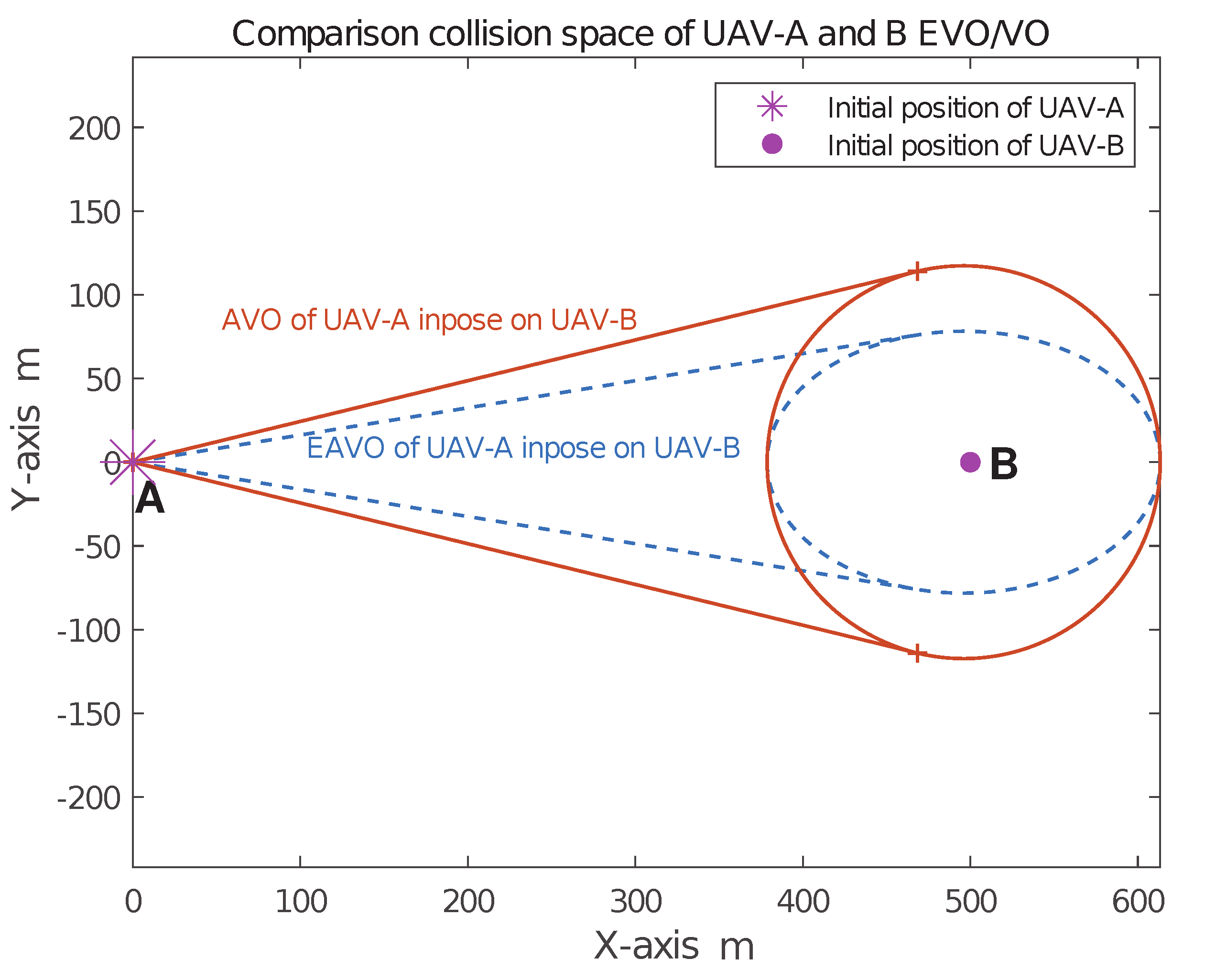
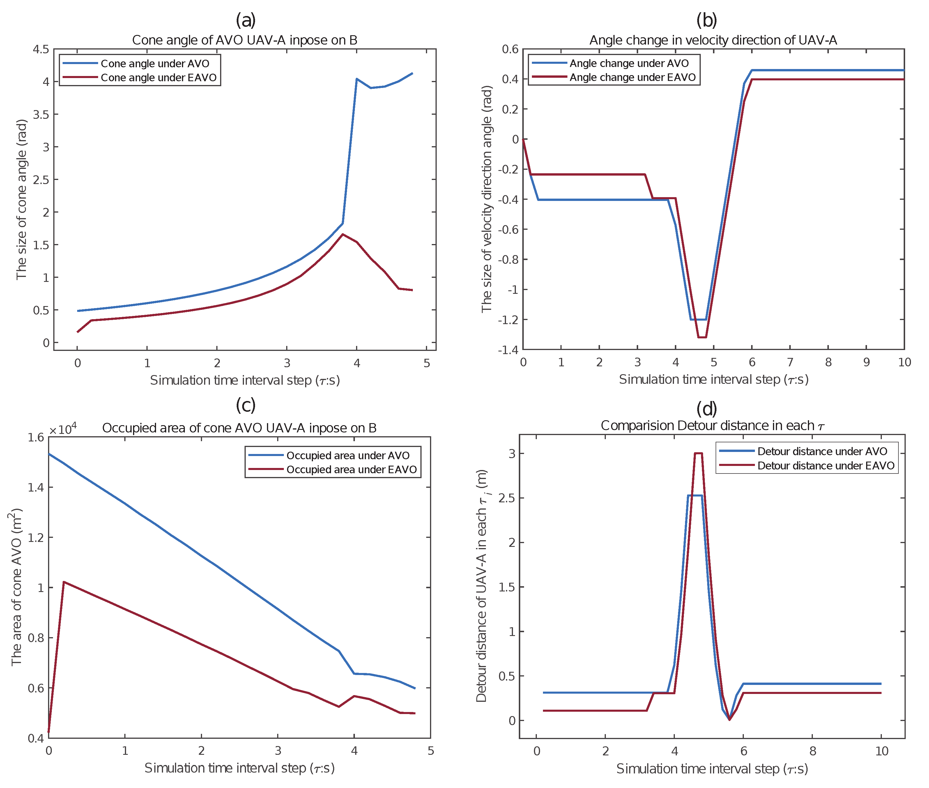
5.3.1. Scenarios 1 Simulation Experiment

It can be seen that both protection domain assumptions achieve obstacle avoidance resolution for this pair of UAVs (Figure 12a,b). The flight trajectory of UAV-A under the elliptical assumption is smoother (Figure 12c,d). Based on the distance between A and B throughout the flight (Figure 13a,b), it is clear that the closest distance between the two is much closer under the elliptic domain assumption. Since the length of protection is the same in all circle domain directions, a separation distance of nearly ‘2a’ between drones is actually more dangerous. For the elliptic assumption, as the orientation of UAV-A changes, the elliptic protection domain also changes, and the actual distance between A and B is less than ‘2a’ but still outside the elliptic domain (Figure 13a green dashed line). Therefore, the result for the circle domain is clearly more conservative.

It can be seen that the cone angle of the VO of the circle domain assumption is always above the elliptic domain assumption (Figure 14a), indicating that using the circle domain assumption requires a larger angle of deflection to complete the unwinding. The VO of the circle domain assumption occupies a larger area of the space and squeezes more of the free space, while the elliptic domain contributes more of the non-conflicting space (Figure 14c). Since the deflection angle of A under the circle domain assumption is greater (Figure 14b), the resulting detour distance in each simulation interval $\tau$ is also larger (Figure 14d). Additionally, it is evident that UAV-A’s velocity adjustment does not enter an oscillatory loop. It merely executes a few obstacle avoidance maneuvers before resuming a stable flight. It then continues to monitor for collision risks, making adjustments successively as necessary (Figure 14b).

The observed results stem from the smaller velocity obstacle space within the elliptical domain, which provides a broader range of optional velocities. This additional velocity selection, which would be unfeasible under the circle domain assumption, will become feasible under the elliptical domain, often requiring only small adjustments. In contrast, under the circle domain hypothesis, a significant portion of the potential obstacle avoidance directions might be prematurely excluded due to the larger space and the greater angle at the top of the obstacle cone.

5.3.2. Scenarios 2 Simulation Experiment

Next, the distance between A and B was adjusted to 200 m. We repeated the procedure according to the experimental conditions in Scenario 2. In Scenario 2, where the spacing is more constrained, the effectiveness of the velocity adjustments by UAV-A within the elliptical domain assumption becomes more apparent. This setup allows UAV-A to avoid obstacles with smaller angular deflections as it approaches UAV-B. However, Figure 15a–d confirms that the purple and green elliptical domains do not overlap at any point, which is facilitated by the lack of inherent arbitrary rotational symmetry to ellipses. Figure 16a,b in the spacing distance curve shows that under the elliptical assumption, UAVs A and B are closer together compared to when operating under the circle domain assumption, falling between the lengths of the major and minor axes. Meanwhile, the circle domain maintains a constant safety interval of 2a at all times, ensuring the distance between A and B remains above this threshold, which necessitates a larger detour.

The overall indicators for Scenarios 1 and 2 are summarized in

Table 3. Overall indicators and velocity reback moment.

Pre-Set Scenario	Domain Hypothesis	Total Detour Distanc (m)	Single Obstacle Avoidance Time (s)	Velocity Reback Moment (s)
Scenario 1	Elliptic domain	54.37	0.0016	${\tau }_{\mathrm{reback}}=61\tau =12.2$
	Circle domain	69.29	0.00056	${\tau }_{\mathrm{reback}}=62\tau =12.4$
Scenario 2	Elliptic domain	44.96	0.0043	${\tau }_{\mathrm{reback}}=13\tau =2.6$
	Circle domain	56.65	0.0014

. It can be seen that under the scenarios with different distance scales, the total detour distance of the UAV structured in the elliptic domain is smaller than that in the circle domain throughout the obstacle avoidance process. In terms of the time efficiency of a single resolution, although the VO space computation of the elliptic domain is much more complicated than that of the circle domain, the method of calling the convhull function for discrete elliptic boundary nodes proposed in this paper does not significantly lag behind. And, both of them almost reach the critical reback moment when A and B pass by each other at the same time.

Based on Figure 17a–d, we can obtain similar conclusions in Scenario 1. The results of obstacle avoidance under the elliptic domain structure are more superior in Scenario 2, which is reflected in the compression of the total detour distance and the improvement of the computational efficiency in Table 3. Because the initial A and B separation distance is reduced from 500 m to 200 m, the ellipse assumption still saves about 10 m of extra detours.

We can foresee that when the two UAVs are closer together and the size of the protection domain obtained in Section 3.3 is smaller than the protection domain required by the actual physical properties of the UAVs, a situation may occur where the circle protection domain is unable to avoid obstacles, while the elliptical domain can avoid obstacles. Assuming that this minimum physical protection domain is a = 20 m, b = 10 m, we test it when the distance between UAVs A and B is 80 or 100 m, and the other parameters are consistent with Scenario 2. The actual experiments demonstrated that when the protection domain fixed the UAV’s velocity in the direction of the major axis, it was not effective for obstacle avoidance. The circular domain structure also failed in the 80m scenario. On the contrary, interchanging the values of a and b yields the desired results (Figure 18a–f). This suggests that timely changes in the axial orientation of the elliptic domain are needed to better accommodate narrow scenarios of obstacle avoidance.

5.4. Defects of Custom Elliptic Domains for Proximity UAVs

When the drones are in close proximity, the custom elliptic domain we proposed will also become trapped in a dilemma during obstacle avoidance. During the experimental phase, both elliptic and circle domains produced mutual intrusions at 100 and 80 m. Figure 18 indicates that with the movement of the UAV, our aim to provide a larger protection domain for the velocity direction gradually became inapplicable, and the relative positional relationship between the two should be considered in real time. When swapping the values of a and b in the elliptic domains, the UAV’s obstacle avoidance performance in tight scenarios aligned with our expectations for an elliptic domain (Figure 18). This indicates that the elliptic domain, which depends only on the state of conflict at the initial moment and fixes the direction of the velocity as the major axis of the ellipse, will no longer be applicable as the relative positions of the two UAVs change. Therefore, the ideal elliptic domain should be a dynamic protection domain that constantly changes with the relative positions of the conflicting individuals and should always provide a major-axis protection field for the most significant direction of the conflict.

6. Summary and Outlook

This paper explored the types of protective domains that can scientifically achieve safe obstacle avoidance during UAV flight. Fixed-size circle domains often lead to redundancy, which may be feasible when airspace resources are abundant and conflict scales are small. However, in scenarios where UAVs face limited space for maneuvering or when there are numerous conflicting UAVs, large circle domains with a preset radius may prove ineffective. Consequently, this paper investigated elliptic domains and their algorithms to develop a more generalized and efficient protection framework, enhancing safety in complex or crowded flight environments. For unmanned aerial vehicles (UAVs) in head-on conflict scenarios with a specified separation distance, the size of the preset elliptical protection domain can be determined based on the corresponding UAV performance parameters. The obstacle avoidance turning angles can be calculated according to the elliptical domain, allowing the UAVs to return to their flight paths and navigate towards the target point after the conflict risk has been eliminated.

Based on the results obtained, in Scenario 1, where the distance between A and B was large, there were some differences between the circle and elliptical domains in terms of the detour distance. In UAV navigation, the circle domain assumption resulted in a larger velocity obstacle area and more conservatively adjusted velocities. In contrast, the elliptic domain occupies less space and lacks the central symmetry of a circle, causing each deflection to alter the shape of the subsequent velocity obstacle. This alteration affects the uniformity of tangential velocity changes, thereby eliminating the conservatism of the circle domain assumption. In Scenario 2, where the proximity between UAVs A and B was less, the elliptical domain still achieved obstacle avoidance with a decreased detour distance. Moreover, due to the less demanding computation times, the time consumed approached that of the circle domain.

To improve the research process in this paper, we plan to explore and solve these technical problems in the future:

• Custom protection domains for arbitrary flight scenarios

In this paper, we simplified the flight process and reduced the complexity of calculating parameters such as ellipse distance and projection length by setting a research scenario where two UAVs collide head-on while simultaneously dodging in the same deflection velocity direction. This scenario restricts the applicability of the derived ellipse protection domain sizes to head-on collisions only. For collisions at varying angles, the complexity of motion and rotation within the elliptic structure may significantly increase. It requires us to develop a design algorithm that is suitable for more general scenarios and fast enough for planning.

• The lower limit of the elliptic protection domain

In this paper, the size of the custom elliptic domain was determined based on interval distance between UAVs A and B, the actual velocity, and the angular velocity. As the interval distance decreases, the model-derived protection domain may become excessively small, suggesting the need for a minimum protection domain size based on the actual physical properties of the UAVs. If the domain size falls below this threshold, the UAVs may disrupt each other’s flight stability due to airflow interference. Due to the high costs associated with actual UAV field test flights, this paper had not established a lower limit for the protection domain, which presents certain limitations.

• Exploring elliptical domain applications in more complex experimental scenarios

This study is limited to the examination of head-on collision risks for drones in a two-dimensional scenario. The rationale for this foundational assumption is that collisions between drones flying directly toward each other are deterministic and that their collision points are easily identifiable. This ensures that critical conditions for avoiding collisions can be readily derived, facilitating the analysis of the obstacle avoidance flight process using elliptical domains. It allows for easier consideration of nonlinear velocity adjustments during the deflection process of the velocity obstacle method and the resulting endpoint errors in obstacle avoidance flight positions. In contrast, establishing a quantitative functional relationship between the size of the elliptical protection domain and the obstacle avoidance process for drones in arbitrary flight states, such as non-collinear uniform linear motion or variable speed curve flights, poses significant challenges. Therefore, more complex obstacle environments, such as multiple static obstacles, drones following arbitrary curved flight paths, and multiple drones engaged in obstacle avoidance, have not been addressed in this paper.

Moreover, in real-world flight scenarios for drones, especially those with smaller geometric dimensions, they are highly susceptible to spatial gusts. When considering wind factors, the navigation of the drone may need to satisfy various constraints related to kinematics, dynamics, communication connectivity, and obstacle avoidance. Wind disturbances require the planning process to continuously update and generate new trajectories. Control barrier functions (CBFs) are used to assist in collision avoidance in the face of wind disturbances while alleviating the need to continually recalculate the motion plans [45]. Additionally, Phadke [46] established a disruption model considering obstacles and wind factors across multiple scenarios, and its experimental results provide important insights for assessing whether drones can navigate safely amid environmental disturbances. In this paper, if external factors such as wind are taken into account, assessing the degree of spatial positional uncertainty or increased collision risk level due to wind, quantifying it into the spatial extent of a customized ellipsoidal domain, and superimposing it on an existing ellipsoidal domain is a research direction that can be explored.

In the future, we plan to further improve and refine the elliptic domain setting algorithm to correlate with the real-time relative positions of the conflicting objects with respect to the above two problems. In addition, we plan to explore the best obstacle avoidance position eliminating velocity oscillations and verify the superior conflict resolution performance of the elliptic domains in narrower or crowded multi-UAV situations.

References

1. Fu, Q.; Liang, X.; Zhang, J.; Hou, Y. Cooperative conflict detection and resolution for multiple UAVs using two-layer optimization. Harbin Gongye Daxue Xuebao/J. Harbin Inst. Technol. 2020, 52, 74–83. [Google Scholar]
2. Sarim, M.; Radmanesh, M.; Dechering, M.; Kumar, M.; Pragada, R.; Cohen, K. Distributed detect-and-avoid for multiple unmanned aerial vehicles in national air space. J. Dyn. Syst. Meas. Control 2019, 141, 071014. [Google Scholar] [CrossRef]
3. Sunberg, Z.N.; Kochenderfer, M.J.; Pavone, M. Optimized and trusted collision avoidance for unmanned aerial vehicles using approximate dynamic programming. In Proceedings of the 2016 IEEE International Conference on Robotics and Automation (ICRA), Stockholm, Sweden, 16–21 May 2016; IEEE: New York, NY, USA, 2016; pp. 1455–1461. [Google Scholar]
4. Phung, M.D.; Ha, Q.P. Safety-enhanced UAV path planning with spherical vector-based particle swarm optimization. Appl. Soft Comput. 2021, 107, 107376. [Google Scholar] [CrossRef]
5. Pehlivanoglu, Y.V.; Pehlivanoglu, P. An enhanced genetic algorithm for path planning of autonomous UAV in target coverage problems. Appl. Soft Comput. 2021, 112, 107796. [Google Scholar] [CrossRef]
6. Hao, G.; Lv, Q.; Huang, Z.; Zhao, H.; Chen, W. UAV Path Planning Based on Improved Artificial Potential Field Method. Aerospace 2023, 10, 562. [Google Scholar] [CrossRef]
7. Liu, Y.; Zhao, Y. A virtual-waypoint based artificial potential field method for UAV path planning. In Proceedings of the 2016 IEEE Chinese Guidance, Navigation and Control Conference (CGNCC), Nanjing, China, 12–14 August 2016; IEEE: New York, NY, USA, 2016; pp. 949–953. [Google Scholar]
8. Pan, Z.; Zhang, C.; Xia, Y.; Xiong, H.; Shao, X. An Improved Artificial Potential Field Method for Path Planning and Formation Control of the Multi-UAV Systems. IEEE Trans. Circuits Syst. II Express Briefs 2022, 69, 1129–1133. [Google Scholar] [CrossRef]
9. Fiorini, P.; Shiller, Z. Motion planning in dynamic environments using velocity obstacles. Int. J. Robot. Res. 1998, 17, 760–772. [Google Scholar] [CrossRef]
10. Best, A.; Narang, S.; Manocha, D. Real-time reciprocal collision avoidance with elliptical agents. In Proceedings of the 2016 IEEE International Conference on Robotics and Automation (ICRA), Stockholm, Sweden, 16–21 May 2016; IEEE: New York, NY, USA, 2016; pp. 298–305. [Google Scholar]
11. Guo, H.; Guo, X. Local path planning algorithm for UAV based on improved velocity obstacle method. Hangkong Xuebao/Acta Aeronaut. et Astronaut. Sin. 2023, 44, 327586. [Google Scholar]
12. Bi, K.; Wu, M.; Zhang, W.; Wen, X.; Du, K. Modeling and analysis of flight conflict network based on velocity obstacle method. Xi Tong Gong Cheng Yu Dian Zi Ji Shu/Syst. Eng. Electron. 2021, 43, 2163–2173. [Google Scholar]
13. Zhang, H.; Gan, X.; Li, A.; Gao, Z.; Xu, X. UAV obstacle avoidance and track recovery strategy based on velocity obstacle method. Xi Tong Gong Cheng Yu Dian Zi Ji Shu/Syst. Eng. Electron. 2020, 42, 1759–1767. [Google Scholar]
14. Yang, W.; Wen, X.; Wu, M.; Bi, K.; Yue, L. Three-Dimensional Conflict Resolution Strategy Based on Network Cooperative Game. Symmetry 2022, 14, 1517. [Google Scholar] [CrossRef]
15. Peng, M.; Meng, W. Cooperative obstacle avoidance for multiple UAVs using spline_VO method. Sensors 2022, 22, 1947. [Google Scholar] [CrossRef]
16. Adouane, L.; Benzerrouk, A.; Martinet, P. Mobile robot navigation in cluttered environment using reactive elliptic trajectories. IFAC Proc. Vol. 2011, 44, 13801–13806. [Google Scholar] [CrossRef]
17. Braquet, M.; Bakolas, E. Vector field-based collision avoidance for moving obstacles with time-varying elliptical shape. IFAC-PapersOnLine 2022, 55, 587–592. [Google Scholar] [CrossRef]
18. Gérin-Lajoie, M.; Richards, C.L.; McFadyen, B.J. The negotiation of stationary and moving obstructions during walking: Anticipatory locomotor adaptations and preservation of personal space. Mot. Control 2005, 9, 242–269. [Google Scholar] [CrossRef]
19. Chraibi, M.; Seyfried, A.; Schadschneider, A. Generalized centrifugal-force model for pedestrian dynamics. Phys. Rev. E 2010, 82, 046111. [Google Scholar] [CrossRef] [PubMed]
20. Lee, B.H.; Jeon, J.D.; Oh, J.H. Velocity obstacle based local collision avoidance for a holonomic elliptic robot. Auton. Robot. 2017, 41, 1347–1363. [Google Scholar] [CrossRef]
21. Wang, G.; Liu, M.; Wang, F.; Chen, Y. A novel and elliptical lattice design of flocking control for multi-agent ground vehicles. IEEE Control Syst. Lett. 2022, 7, 1159–1164. [Google Scholar] [CrossRef]
22. Du, Z.; Li, W.; Shi, G. Multi-USV Collaborative Obstacle Avoidance Based on Improved Velocity Obstacle Method. ASCE-ASME J. Risk Uncertain. Eng. Syst. Part A Civ. Eng. 2024, 10, 04023049. [Google Scholar] [CrossRef]
23. Mao, S.; Yang, P.; Gao, D.; Bao, C.; Wang, Z. A Motion Planning Method for Unmanned Surface Vehicle Based on Improved RRT Algorithm. J. Mar. Sci. Eng. 2023, 11, 687. [Google Scholar] [CrossRef]
24. Singh, Y.; Sharma, S.; Sutton, R.; Hatton, D.; Khan, A. A constrained A* approach towards optimal path planning for an unmanned surface vehicle in a maritime environment containing dynamic obstacles and ocean currents. Ocean Eng. 2018, 169, 187–201. [Google Scholar] [CrossRef]
25. Liu, Y.; Bucknall, R. Path planning algorithm for unmanned surface vehicle formations in a practical maritime environment. Ocean Eng. 2015, 97, 126–144. [Google Scholar] [CrossRef]
26. Munasinghe, S.R.; Oh, C.; Lee, J.J.; Khatib, O. Obstacle avoidance using velocity dipole field method. In Proceedings of the International Conference on Control, Automation, and Systems, ICCAS, Budapest, Hungary, 26–29 June 2005; pp. 1657–1661. [Google Scholar]
27. Abdallaoui, S.; Aglzim, E.H.; Kribeche, A.; Ikaouassen, H.; Chaibet, A.; Abid, S.E. Dynamic and Static Obstacles Avoidance Strategies Using Parallel Elliptic Limit-Cycle Approach for Autonomous Robots. In Proceedings of the 2023 11th International Conference on Control, Mechatronics and Automation (ICCMA), Agder, Norway, 1–3 November 2023; IEEE: New York, NY, USA, 2023; pp. 133–138. [Google Scholar]
28. Shiller, Z.; Large, F.; Sekhavat, S. Motion planning in dynamic environments: Obstacles moving along arbitrary trajectories. In Proceedings of the 2001 ICRA. IEEE International Conference on Robotics and Automation (Cat. No. 01CH37164), Seoul, Republic of Korea, 21–26 May 2001; IEEE: New York, NY, USA, 2001; Volume 4, pp. 3716–3721. [Google Scholar]
29. Large, F.; Laugier, C.; Shiller, Z. Navigation among moving obstacles using the NLVO: Principles and applications to intelligent vehicles. Auton. Robot. 2005, 19, 159–171. [Google Scholar] [CrossRef]
30. Chen, P.; Huang, Y.; Mou, J.; Van Gelder, P. Ship collision candidate detection method: A velocity obstacle approach. Ocean Eng. 2018, 170, 186–198. [Google Scholar] [CrossRef]
31. Chen, P.; Huang, Y.; Papadimitriou, E.; Mou, J.; van Gelder, P. An improved time discretized non-linear velocity obstacle method for multi-ship encounter detection. Ocean Eng. 2020, 196, 106718. [Google Scholar] [CrossRef]
32. Van den Berg, J.; Lin, M.; Manocha, D. Reciprocal velocity obstacles for real-time multi-agent navigation. In Proceedings of the 2008 IEEE International Conference on Robotics and Automation, Pasadena, CA, USA, 19–23 May 2008; IEEE: New York, NY, USA, 2008; pp. 1928–1935. [Google Scholar]
33. Van Den Berg, J.; Guy, S.J.; Lin, M.; Manocha, D. Reciprocal n-body collision avoidance. In Robotics Research: The 14th International Symposium ISRR; Springer: Berlin/Heidelberg, Germany, 2011; pp. 3–19. [Google Scholar]
34. Han, R.; Chen, S.; Wang, S.; Zhang, Z.; Gao, R.; Hao, Q.; Pan, J. Reinforcement learned distributed multi-robot navigation with reciprocal velocity obstacle shaped rewards. IEEE Robot. Autom. Lett. 2022, 7, 5896–5903. [Google Scholar] [CrossRef]
35. Giese, A.; Latypov, D.; Amato, N.M. Reciprocally-rotating velocity obstacles. In Proceedings of the 2014 IEEE International Conference on Robotics and Automation (ICRA), Hong Kong, China, 31 May–7 June 2014; IEEE: New York, NY, USA, 2014; pp. 3234–3241. [Google Scholar]
36. JEON, J.D. A Velocity-Based Local Navigation Approach to Collision Avoidance of Elliptic Robots. Ph.D. Thesis, Seoul National University, Seoul, Republic of Korea, 2017. [Google Scholar]
37. Feurtey, F. Simulating the Collision Avoidance Behavior of Pedestrians; The University of Tokyo, School of Engineering, Department of Electronic Engineering: Tokyo, Japan, 2000. [Google Scholar]
38. Snape, J.; Van Den Berg, J.; Guy, S.J.; Manocha, D. The hybrid reciprocal velocity obstacle. IEEE Trans. Robot. 2011, 27, 696–706. [Google Scholar] [CrossRef]
39. Snape, J.; Van Den Berg, J.; Guy, S.J.; Manocha, D. Independent navigation of multiple mobile robots with hybrid reciprocal velocity obstacles. In Proceedings of the 2009 IEEE/RSJ International Conference on Intelligent Robots and Systems, St. Louis, MO, USA, 11–15 October 2009; IEEE: New York, NY, USA, 2009; pp. 5917–5922. [Google Scholar]
40. Kavraki, L.E. Computation of configuration-space obstacles using the fast Fourier transform. IEEE Trans. Robot. Autom. 1995, 11, 408–413. [Google Scholar] [CrossRef]
41. Lee, I.K.; Kim, M.S.; Elber, G. Polynomial/rational approximation of Minkowski sum boundary curves. Graph. Model. Image Process. 1998, 60, 136–165. [Google Scholar] [CrossRef]
42. Wein, R. Exact and efficient construction of planar Minkowski sums using the convolution method. In European Symposium on Algorithms; Springer: Berlin/Heidelberg, Germany, 2006; pp. 829–840. [Google Scholar]
43. Yan, Y.; Chirikjian, G.S. Closed-form characterization of the Minkowski sum and difference of two ellipsoids. Geom. Dedicata 2015, 177, 103–128. [Google Scholar] [CrossRef]
44. Cheng, Z.; Chen, P.; Mou, J.; Chen, L. Multi-ship Encounter Situation Analysis with the Integration of Elliptical Ship Domains and Velocity Obstacles. TransNav. Int. J. Mar. Navig. Saf. Od Sea Transp. 2023, 17, 895–902. [Google Scholar] [CrossRef]
45. Abichandani, P.; Lobo, D.; Muralidharan, M.; Runk, N.; McIntyre, W.; Bucci, D.; Benson, H. Distributed Motion Planning for Multiple Quadrotors in Presence of Wind Gusts. Drones 2023, 7, 58. [Google Scholar] [CrossRef]
46. Phadke, A.; Medrano, F.A.; Chu, T.; Sekharan, C.N.; Starek, M.J. Modeling Wind and Obstacle Disturbances for Effective Performance Observations and Analysis of Resilience in UAV Swarms. Aerospace 2024, 11, 237. [Google Scholar] [CrossRef]
Figure 1. Schematic of research process and architecture.
Drones 08 00397 g001
Figure 2. Schematic of AVO between equal-radius circle domains.
Drones 08 00397 g002
Figure 3. Station α 0 : Two of the same circular domain collisions.
Drones 08 00397 g003
Figure 4. Station α 1 : Two different circular domain collisions.
Drones 08 00397 g004
Figure 5. Station α 2 : Two of the same internal elliptical collisions.
Drones 08 00397 g005
Figure 6. Station α 3 : Two of the same external elliptical collisions.
Drones 08 00397 g006
Figure 7. Schematic of UAV conflict risk phase and conflict risk elimination phase flights.
Drones 08 00397 g007
Figure 8. Schematic illustration of possible collisions during the UAVs’ conflict risk phase.
Drones 08 00397 g008
Figure 9. Schematic of flight endpoints under the three assumptions in the conflict risk phase.
Drones 08 00397 g009
Figure 10. Schematic of displacement endpoint errors Δ s and d e analysis.
Drones 08 00397 g010
Figure 11. Initial moment AVO, EAVO in scenarios 1.
Drones 08 00397 g011
Figure 12. EAVO/AVO space and flight position in scenario 1.
Drones 08 00397 g012
Figure 13. Comparison of flight distances in scenario 1.
Drones 08 00397 g013
Figure 14. Comparison of process indicators in scenario 1.
Drones 08 00397 g014
Figure 15. EAVO/AVO space and flight position in scenario 2.
Drones 08 00397 g015
Figure 16. Comparison of flight distances in scenario 2.
Drones 08 00397 g016
Figure 17. Comparison of process indicators in scenario 2.
Drones 08 00397 g017
Figure 18. Comparison of protection domain obstacle avoidance results at 100 and 80 m.
Drones 08 00397 g018