Pseudospectral-Based Rapid Trajectory Planning and Feedforward Linearization Guidance

Abstract

A trajectory-based guidance strategy is proposed for the three-dimensional terminal return task of an uncrewed space vehicle (USV). The overall guidance scheme consists of reference trajectory planning and robust trajectory tracking modules. The trajectory planning algorithm involves determining the motion of the USV to achieve a prescribed target under multiple constraints. The altitude-domain-based USV model is firstly proven to be differentially flat utilizing the dynamic pressure and position of the USV as flat outputs. The original trajectory planning problem is reformulated in a lower-dimensional flat output space. The discretization of the planning problem is then achieved using the pseudospectral method, based on which an initial guess technique is designed in order to accelerate the solving speed of the planning algorithm. Subsequently, a feedforward linearization-based trajectory tracking guidance law is designed using the differential flatness property of the altitude-domain model. Simulation results in different scenarios show that the proposed guidance strategy provides a satisfactory guidance solution.

1. Introduction

With the increasing demand for space exploration and transportation, the reusable uncrewed space vehicle (USV) was developed, which has great potentials in reducing costs and increasing flexibility [1,2]. Re-entry flight is one of the crucial technologies for a safe return, which largely determines the reusable capability of a USV [3,4]. A re-entry flight usually consists of three stages, including the initial re-entry (IRE) phase, terminal area energy management (TAEM) phase, and approach and landing (A&L) phase [5]. The IRE phase is a hypersonic phase from an altitude of 400 kft to a TAEM entry point around 100 kft. In the TAEM phase, the USV flies from an altitude of around 100 kft with the velocity of Mach 2.5 down to the TAEM terminal point with 10 kft and Mach 0.5. Then, the A&L phase completes the final re-entry task from Mach 0.5 down to runway touch point [6,7]. Of the three flight stages, the TAEM phase faces some different challenges than the other two phases. For example, large lateral maneuver is required for the USV to dissipate the high energy of the USV since the velocity and altitude are still high at the end of the IRE phase. On the other hand, the USV is generally unpowered (i.e., without thrust) at the TAEM phase in order to carry more payloads to perform exploration missions. This asks for high requirements in terms of the guidance reliability. In addition, at the end of a TAEM flight, the USV should align with the runway in high precision for the convenience of the following A&L phase. This means that high terminal guidance accuracy is required.

The first TAEM guidance system was proposed for the Space Shuttle program, where the trajectory was designed with a ground track composed of several separate sub-phases, including S-turn, acquisition, a heading alignment cylinder (HAC), and a pre-final approach [8]. This method is essentially a decoupling strategy. The guidance performance in terms of operational flexibility, the terminal guidance precision, and robustness to disturbance needs to be further enhanced. To address these issues, some improved guidance strategies have been studied. A three-dimensional trajectory planning algorithm is presented in [9]. A dynamic pressure profile was designed to meet the longitudinal constraints, and a correction method was used to adjust the lateral position of the USV. In [10], a TAEM guidance method with a predicted ground track profile is proposed. A feasible gliding trajectory is obtained by optimizing three parameters. Subsequently, a decoupling PID guidance law is used to track the trajectory. On this basis, the optimal trajectory is selected in [11]. In [12], a TAEM trajectory optimization algorithm is designed, and a global optimal solution can be achieved based on the proposed interval analysis approach. In [13], the capability of energy management during the terminal phase of the USV is analyzed, and the best HAC position can be obtained using the energy-tube-based planning algorithm. In [14,15], the offline longitudinal trajectories are predesigned, and the online correction strategy is then used to adjust the lateral trajectory. In [16], a guidance parameter iteration strategy is designed to obtain the optimal TAEM trajectory. In [17], the gliding range of the USV during the TAEM phase is calculated with consideration of different initial flight states. In [18], the longitudinal trajectory is designed considering constraints on the Mach number, and the lateral states are corrected using numerical techniques. Changes in the initial conditions are considered in [17,18]. But other types of deviations, such as atmospheric or aerodynamic uncertainties, are not taken into account. In [19], a new ground track for TAEM phase is designed combining the heading alignment cylinder (HAC) with an energy dissipation circle. In [20], a longitudinal profile is designed based on the requirements of the flight path angle. In [21], an HAC radius adjustment algorithm is designed to meet the requirement of the terminal energy of the USV.

Various degrees of success have been achieved by the discussed studies. Nevertheless, they follow the design routine of the Shuttle to a large extent. Complicated geometric ground track segments are utilized. This might lead to low flexibility and poor robustness in the presence of large uncertainties, such as aerodynamic deviations, terminal entry errors, etc. Hence, advanced guidance technology, which can adapt appropriately to unfavorable varying circumstances and handle large parametric uncertainties, is needed to improve mission flexibility and operation autonomy for a USV. With the rapid development in computational power and numerical algorithms, optimization-based trajectory planning and adaptive guidance strategies have drawn increasing attention in various fields of the flight vehicle, such as in the A&L phase of the reusable USV [22], IRE phase of the reusable USV [3,23,24,25], reconnaissance task of an aeroassisted vehicle [26], recovery task of the USV [27], vertical landing task of the rocket [28,29], maneuvering trajectory of aircraft [30,31], and so on. Among them, the differential flatness-based planning method is a new solution for the optimization-based trajectory optimization, which has advantages in reducing the optimization dimension and improving efficiency. In [32], a trajectory planning algorithm is proposed for a hypersonic glide vehicle during a hypersonic re-entry phase (skipping gliding phase) based on differential flatness theory and the mapped Chebyshev pseudospectral method. In [33], a trajectory optimization approach is proposed for a reusable launch vehicle based on differential flatness and direct transcription. In [34], the flatness theory with a B-Spline discretization strategy is designed for the trajectory planning of a USV.

But few three-dimensional trajectory planning-based guidance strategies have been used for the TAEM task due to the fact that complex constraints should be considered during the return. In this paper, a new pseudospectral-based rapid trajectory planning and feedforward linearization guidance strategy is presented for the TAEM phase. The guidance precision and robustness are substantially enhanced since multiple constraints are counted for the trajectory design together with a robust tracking law.

The main contributions of the paper lie in three aspects. (1) The gliding dynamic of an unpowered USV is transformed into the domain of altitude to extract the main characteristic in the TAEM phase. A set of flat outputs can thereby be determined. Based on this treatment, trajectory planning is handled in a lower-dimensional space. Furthermore, this brings in the benefit that the variable to be optimized is directly related to the requirement of the TAEM task, while the final flight time, which is commonly an optimization variable, is removed. And the objective function can also be flexibly designed according to the specific task. (2) The optimal control-based TAEM trajectory planning problem is transformed into a nonlinear programming problem using flat outputs at discrete nodes as decision variables. Meanwhile, a new initial guess strategy is proposed by integrating the advantage of the pseudospectral method. The generated trajectory can satisfy the multiple constraints for the TAEM flight. (3) A feedforward linearization and extended proportional–integral–derivative (PID) guidance law is designed based on the differential flatness property. This strategy can provide adaptation to model uncertainties using only part of the system states.

The rest of this paper is organized as follows. Section 2 describes the mathematical model of a USV and statement of the TAEM guidance problem. Section 3 presents the overall structure of the proposed TAEM guidance strategy. In Section 4, an altitude-domain motion equation is first derived, followed by an extension of the flatness property. In Section 5, the trajectory planning problem is established based on the new guidance model and its differential flatness. It is then discretized using the pseudospectral method. In Section 6, the problem is solved with an initialization strategy. Section 7 develops a trajectory tracking law via feedforward linearization and extended PID techniques. Section 8 demonstrates the performance of the proposed guidance scheme considering different flight scenarios. Section 9 concludes this paper.

2. Preliminaries

In this section, the gliding dynamic model of the USV is presented, followed by the problem description of the USV terminal gliding phase.

2.1. Mathematical Model of Reusable USV in TAEM Phase

With the assumption that the Earth is flat and the USV is unpowered, the model capturing the gliding dynamics of a USV can be represented as follows [6]:

$$\mathrm{d}x/\mathrm{d}t=Vcos\gamma cos\chi ,$$

(1)

$$\mathrm{d}y/\mathrm{d}t=Vcos\gamma sin\chi ,$$

(2)

$$\mathrm{d}h/\mathrm{d}t=Vsin\gamma ,$$

(3)

$$\mathrm{d}V/\mathrm{d}t=-D/m-gsin\gamma ,$$

(4)

$$\mathrm{d}\gamma /\mathrm{d}t=Lcos\mu /\left(mV\right)-gcos\gamma /V,$$

(5)

$$\mathrm{d}\chi /\mathrm{d}t=Lsin\mu /\left(mVcos\gamma \right),$$

(6)

where x and y represent the down-track and cross-track position, respectively. h is the altitude of the USV. V is the velocity of the USV. $\gamma$ and $\chi$ are the flight path and heading angle, respectively. $\mu$ is the bank angle. m is the vehicle mass. g is the gravitational acceleration. L and D denote the lift and drag force, respectively, which are computed by multiplying the dynamic pressure q by the reference area S and the aerodynamic coefficients $C_L$ and $C_D$, respectively:

$$L=qS{C}_L,$$

(7)

$$D=qS{C}_D,$$

(8)

with

$$q=0.5\rho V^2,$$

(9)

where $\rho$ is the atmospheric density. In addition, $C_L$ and $C_D$ can be expressed by the angle of attack $\alpha$ and Mach number M using polynomial approximations as below:

$$C_L=a_0\left(M\right)+a_1\left(M\right)\alpha +a_2\left(M\right){\alpha }^2,$$

(10)

$$C_D=b_0\left(M\right)+b_1\left(M\right)\alpha +b_2\left(M\right){\alpha }^2+k\left(M\right)\delta ,$$

(11)

where $a_j(j=0,1,2)$ and $b_j(j=0,1,2)$ are the polynomial parameters obtained by fitting several sets of discrete data including the values of the aerodynamic coefficients and Mach numbers. For different Mach numbers within the range of $[0.5,2.5]$, the polynomial function coefficients are different. $k\left(M\right)$ indicates how much the speedbrake $\delta$ influences the drag coefficient $C_D$. The detailed coefficients can be found in [35].

In the above mathematical model of the USV, it can be observed that $\alpha$, $\mu$, and $\delta$ are the inputs. The model can be written in the nonlinear ordinary differential equation form of

$${\dot{\mathit{x}}}_{\mathit{t}}\mathbf{=}{\mathit{f}}_{\mathit{t}}\mathbf{(}{\mathit{x}}_{\mathit{t}}\mathbf{,}\mathit{u}\mathbf{)}\mathbf{,}$$

(12)

where the input vector u =${[\alpha ,\mu ,\delta ]}^T$ and the system state $x_t={[x,y,h,V,\gamma ,\chi ]}^T$.

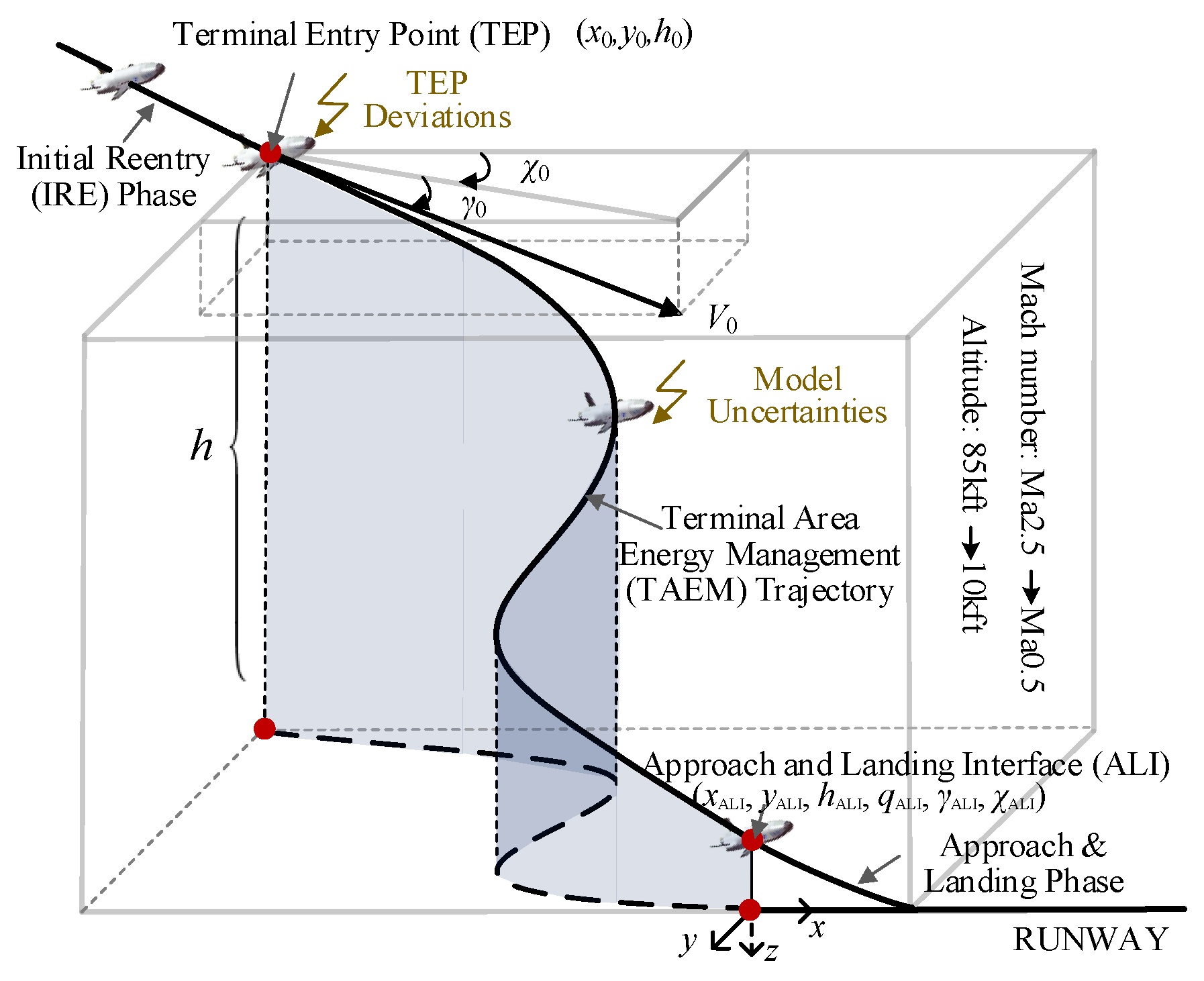
2.2. Description of the TAEM Guidance Problem

The goal of the guidance task in the TAEM phase is to drive the unpowered USV from the terminal entry point (TEP) to the approach and landing interface (ALI), as depicted in Figure 1. Note that the traditional notion of a segmented trajectory [8,15] for the TAEM phase is avoided in this paper. Instead, a consecutive trajectory is expected to be generated.

At the ALI, the energy of the USV is required to be dissipated to a lower desired value, which can be expressed using the altitude and velocity (or dynamic pressure) in terms of $h_{\mathrm{ALI}}$ and $q_{\mathrm{ALI}}$. And it is demanded to align the USV with the runway in order for safe approach and landing flight hereafter. That is, the final kinematic state of the USV should satisfy certain constraints ($x_{\mathrm{ALI}},y_{\mathrm{ALI}},{\chi }_{\mathrm{ALI}},{\gamma }_{\mathrm{ALI}}$). The initial conditions at the TEP might suffer from deviations induced by the error at the end of the IRE phase. This situation together with the model uncertainties should be considered in the TAEM guidance design. On the other hand, during the TAEM flight, the USV must satisfy the vehicle constraints on the dynamic pressure considering the gliding capability and vehicle structural constraint, which can be described by $q\in [q_{min},q_{max}]$. All these constraints are presented in

Table 1. TAEM guidance constraints.

Types	Variables	Constraints
State	Dynamic pressure $q,psf$	$[q_{min},q_{max}]$
Terminal energy	Altitude $h_f,ft$	$h_{\mathrm{ALI}}$
	Dynamic pressure $q_f,psf$	$q_{\mathrm{ALI}}$
Terminal task	Cross-track position $x_f,ft$	$x_{\mathrm{ALI}}$
	Down-track position $y_f,ft$	$y_{\mathrm{ALI}}$
	Heading angle ${\chi }_f,deg$	${\chi }_{\mathrm{ALI}}$
	Flight path angle ${\gamma }_f,deg$	${\gamma }_{\mathrm{ALI}}$

.

3. TAEM Guidance Strategy Design

In the proposed TAEM guidance strategy, two modules are included: reference trajectory generation and robust tracking law design, as illustrated in Figure 2.

The first module is used to develop a reference trajectory generator. In this paper, the trajectory planning problem is formulated as an optimal control problem (OCP) with consideration of task requirements and flight dynamics. The OCP is reformulated in a lower-dimensional space based on the differential flatness property of the altitude-domain motion equation. Then, through the pseudospectral method, the OCP is discretized to be a nonlinear programming problem. It is then solved by a sequential quadratic programming (SQP)-based solver. By these means, the constrained TAEM trajectory can be obtained in terms of the flat outputs, which will be regarded as the reference signals of the trajectory tracking module.

The second module is used to design a trajectory tracking law to produce the corresponding guidance commands, aiming to accommodate disturbances including model uncertainties and external disturbances, such as atmospheric disturbances. In this step, the altitude-domain model is firstly used for guidance law design. Then, to evaluate the validation and performance of the proposed guidance strategy, the time-domain model, which represents the real USV gliding dynamics, is used. The generated guidance commands are transferred to the USV time-domain model obtaining the real-time USV flight states.

The altitude-domain motion equation and its flatness property is used as the foundation of the proposed method. Therefore, in Section 4, the altitude-domain-based model is firstly formulated for the USV, followed by the proof of the differential property.

4. Altitude-Domain Motion Equation and Its Flatness Property

To construct the optimal control problem in the lower-dimensional space, in this section, the altitude-domain motion equation of the USV is first derived. Then, the flatness property of the equations is derived.

4.1. Altitude-Domain-Based Model of USV in TAEM Phase

For the USV return task including the TAEM phase, the flight time is usually not a variable of concern. On the contrary, the main variables of concern are altitude, dynamic pressure, etc. Hence, in this paper, the altitude is regarded as an independent variable in guidance law development instead of time. And another crucial variable dynamic pressure is rearranged as the system state. To this end, by taking the derivative of Equation (9) with respect to altitude, one can obtain

$$\mathrm{d}q/\mathrm{d}h=(V^2/2)(\mathrm{d}\rho /\mathrm{d}h)+\rho V(\mathrm{d}V/\mathrm{d}t)(\mathrm{d}t/\mathrm{d}h)$$

(13)

Then, substituting Equations (3), (4), and (9) into Equation (13) achieves

$$\mathrm{d}q/\mathrm{d}h=\left(\mathrm{d}\rho /\left(\rho \mathrm{d}h\right)-\rho S{C}_D/\left(msin\gamma \right)\right)q-\rho g,$$

(14)

During the flight of the TAEM phase, the altitude of the USV keeps decreasing. In considering this fact, a virtual altitude $\overline{h}=h_0-h$ is used to obtain a monotonically increasing format for the independent variable in the ordinary differential equation instead of the real altitude h. Similar transformations can be made to Equations (1), (2), (5), and (6). The new sets of dynamic equations in the domain of altitude are obtained as follows:

$$\mathrm{d}x/\mathrm{d}\overline{h}=-cos\chi /tan\gamma ,$$

(15)

$$\mathrm{d}y/\mathrm{d}\overline{h}=-sin\chi /tan\gamma ,$$

(16)

$$\mathrm{d}q/\mathrm{d}\overline{h}=\left(\mathrm{d}\rho /\left(\rho \mathrm{d}\overline{h}\right)+\rho S{C}_D/\left(msin\gamma \right)\right)q+\rho g,$$

(17)

$$\mathrm{d}\gamma /\mathrm{d}\overline{h}=-\rho /\left(2sin\gamma \right)\left(S{C}_{L}cos\mu /m-gcos\gamma /q\right),$$

(18)

$$\mathrm{d}\chi /\mathrm{d}\overline{h}=-\left(\rho S{C}_{L}sin\mu \right)/\left(msin2\gamma \right),$$

(19)

where the range of $\overline{h}$ is $[{\overline{h}}_0,{\overline{h}}_f]=[0,h_0-h_{\mathrm{ALI}}]$ for the TAEM phase.

Remark 1.

With respect to trajectory propagation issues, a monotonically independent parameter is usually necessary. Time is normally used in many cases since it is linear and steadily increasing. But the total flight time is not the crucial factor for the TAEM phase. On the other hand, for the trajectory optimization problem, an initial solution is a necessity for the algorithm. If a time-domain model is used, it is often hard to set a reasonable initial solution, since the time range is unknown. To overcome this problem, the time is usually normalized. But this strategy induces an additional parameter (i.e., the final time) to be designed which further increases the complexity of the optimization problem. Hence, in this paper, altitude is used as the independent variable. The potential advantage is that no additional parameter is added for the optimization problem, and this might be more convenient for the initialization of the optimization problem. Note that this strategy works for the situation that the altitude is monotonically changing, such as in the TAEM phase and A&L phase. But it is not suitable for the IRE phase where the skipping entry strategy is usually used with a non-monotonically changed altitude.

The transformed model in Equations (15)–(19) will be applied to the TAEM guidance strategy development. For simplicity of notation, the derivative of the state variable with respect to $\overline{h}$ (e.g., ${\displaystyle \frac{\mathrm{d}x}{\mathrm{d}\overline{h}}}$) will be abbreviated as $x\prime$. In choosing system states as $x={[x,y,q,\gamma ,\chi ]}^T$, the altitude-domain model is described in the form of

$$\mathit{x}\mathbf{\prime }\left(\overline{\mathit{h}}\right)=\mathit{f}(\mathit{x}\left(\overline{\mathit{h}}\right),\mathit{u}\left(\overline{\mathit{h}}\right)).$$

(20)

4.2. Flatness Property of Altitude-Domain Model

The altitude-domain model is also used in [9,14]. Nonetheless, only longitudinal dynamics are considered in iteration algorithms, since time consumption is too high and a feasible trajectory solution might be hard to obtain when lateral dynamics are taken into account simultaneously. This paper focuses on generating the trajectories considering all the corresponding flight dynamics including both lateral and longitudinal dynamics. To ensure that the planning problem is solvable and the efficiency can be enhanced, the differential flatness property is excavated for the altitude-domain model, which allows for characterizing the USV dynamics using fewer states.

Differential flatness is essentially a structural property of a system [36]. Recently, it has drawn much attention in different research areas, such as aerial-towed cable systems [37], underactuated rigid spacecraft [38], quadrotor uncrewed aerial vehicles [39,40,41,42,43,44], and planetary planning systems [45]. A system is called flat if a set of outputs can be found, equal in number to the number of inputs, such that all states and inputs can be expressed in terms of those outputs and their derivatives [37,38]. The definition of differential flatness is given [39,41] by the following.

Definition 1.

The nonlinear system

$$\mathit{x}\mathbf{\prime }\mathbf{=}\mathit{f}\mathbf{(}\mathit{x}\mathbf{,}\mathit{u}\mathbf{)}\mathbf{,}\mathit{x}\mathbf{\in }{\mathit{R}}^{\mathit{n}}\mathbf{,}\mathit{u}\mathbf{\in }{\mathit{R}}^{\mathit{m}}\mathbf{(}\mathit{m}\mathbf{\le }\mathit{n}\mathbf{)}\mathbf{,}$$

(21)

is called differentially flat if there exists an m-tuple Φ of functions:

$$\mathit{z}\mathbf{=}\mathbf{\Phi }\mathbf{(}\mathit{x}\mathbf{,}\mathit{u}\mathbf{,}\mathit{u}\mathbf{\prime }\mathbf{,}\mathbf{\dots }\mathbf{,}{\mathit{u}}^{\mathbf{\left(}\mathit{\sigma }\mathbf{\right)}}\mathbf{)}\mathbf{,}$$

(22)

whose components are differentially independent, such that

$$\mathit{x}\mathbf{=}{\mathbf{\Psi }}_{\mathit{x}}\mathbf{(}\mathit{z}\mathbf{,}\mathit{z}\mathbf{\prime }\mathbf{,}\mathbf{\dots }\mathbf{,}{\mathit{z}}^{\mathbf{\left(}\mathit{\eta }\mathbf{\right)}}\mathbf{)}\mathbf{,}$$

(23)

$$\mathit{u}\mathbf{=}{\mathbf{\Psi }}_{\mathit{u}}\mathbf{(}\mathit{z}\mathbf{,}\mathit{z}\mathbf{\prime }\mathbf{,}\mathbf{\dots }\mathbf{,}{\mathit{z}}^{\mathbf{(}\mathit{\eta }\mathbf{+}\mathbf{1}\mathbf{)}}\mathbf{)}\mathbf{,}$$

(24)

where σ and η denote the maximum-order derivative of u in z and z in x. Note that the maximum-order derivative of z in u is $\eta +1$. $z\in {\mathbb{R}}^m$ are called system flat outputs. Based on Definition 1, the following proposition can be achieved.

Proposition 1.

The altitude-domain model of Equations (15)–(19) is flat by choosing down-track position x, cross-track position y, and dynamic pressure q as flat outputs.

Proof. 

Consider the model of Equations (15)–(19). Selecting $x,y$, and q as the flat outputs and denoting them by $z:=(z_1,z_2,z_3)$, respectively, one can obtain

$$\begin{array}{c}\hfill x=z_1,\end{array}$$

(25)

$$\begin{array}{c}\hfill y=z_2,\end{array}$$

(26)

$$\begin{array}{c}\hfill q=z_3.\end{array}$$

(27)

Then, adding the squares of Equations (15) and (16) provides the flight path angle representation in flat outputs:

$$\gamma =-arctan\sqrt{1/(z_1^{\prime 2}+z_2^{\prime 2})},$$

(28)

and dividing Equation (16) by Equation (15) gives the description of the heading angle in terms of the flat outputs:

$$\chi =arctan\left(z_2^{\prime }/z_1^{\prime }\right).$$

(29)

Equations (25)–(29) denote that system states can then be expressed by flat outputs and their derivatives as follows:

$$\mathit{x}={\mathbf{\Psi }}_{\mathit{x}}(\mathit{z},\mathit{z}\mathbf{\prime }).$$

(30)

where

$${\mathbf{\Psi }}_{\mathit{x}}:=\left[\begin{array}{c}{\mathbf{\Psi }}_{\mathit{x}\mathbf{1}}\\ {\mathbf{\Psi }}_{\mathit{x}\mathbf{2}}\\ {\mathbf{\Psi }}_{\mathit{x}\mathbf{3}}\\ {\mathbf{\Psi }}_{\mathit{x}\mathbf{4}}\\ {\mathbf{\Psi }}_{\mathit{x}\mathbf{5}}\end{array}\right]=\left[\begin{array}{c}{\mathit{z}}_{\mathbf{1}}\\ {\mathit{z}}_{\mathbf{2}}\\ {\mathit{z}}_{\mathbf{3}}\\ -\mathbf{arctan}\sqrt{\mathbf{1}/({\mathit{z}}_{\mathbf{1}}^{\prime \mathbf{2}}+{\mathit{z}}_{\mathbf{2}}^{\prime \mathbf{2}})}\\ \mathbf{arctan}\left({\mathit{z}}_{\mathbf{2}}^{\prime }/{\mathit{z}}_{\mathbf{1}}^{\prime }\right)\end{array}\right]$$

(31)

Moreover, the state derivatives with respect to $\overline{h}$ are calculated according to the above description as follows:

$$x\prime =z_1^{\prime },$$

(32)

$$y\prime =z_2^{\prime },$$

(33)

$$q\prime =z_3^{\prime },$$

(34)

$$\gamma \prime =(z_1^{\prime }{z}_1^{″}+z_2^{\prime }{z}_2^{″})/\left((z_1^{\prime 2}+z_2^{\prime 2}+1)\sqrt{z_1^{\prime 2}+z_2^{\prime 2}}\right),$$

(35)

$$\chi \prime =\left(z_1^{\prime }{z}_2^{″}-z_2^{\prime }{z}_1^{″}\right)/\left(z_1^{\prime 2}+z_2^{\prime 2}\right).$$

(36)

Next, the control inputs are expected to be explicated by the flat outputs. To this end, the bank angle $\mu$ is extracted by solving Equations (18) and (19):

$$\mu =arctan\left(\left(2q\chi \prime sin\gamma \right)/\left(2q\gamma \prime tan\gamma -\rho g\right)\right).$$

(37)

Then, using Equations (27), (28), (35), and (36) gives the expression of bank angle $\mu$ in terms of the flat outputs and their derivatives as follows:

$$\mathit{\mu }\mathbf{=}{\mathbf{\Psi }}_{\mathit{u}\mathbf{2}}\mathbf{(}\mathit{z}\mathbf{,}\mathit{z}\mathbf{\prime }\mathbf{,}\mathit{z}\mathbf{″}\mathbf{)}\mathbf{.}$$

(38)

On the other hand, by solving Equations (18) and (19), one can also render

$$C_L=m\sqrt{{(\chi \prime sin2\gamma )}^2+{\left(\left(\rho gcos\gamma \right)/q-2\gamma \prime sin\gamma \right)}^2}/\left(\rho S\right).$$

(39)

Recalling the lift coefficient representation gives

$$C_L=f_{CL}(\alpha ,M),$$

(40)

where the Mach number is determined by the altitude and dynamic pressure. Hence, in combining Equations (39) and (40) and replacing ${\chi }^{\prime }$ with Equation (36) and ${\gamma }_{\prime }$ with Equation (35), a function of angle of attack $\alpha$ can be obtained:

$$\mathit{\alpha }\mathbf{=}{\mathbf{\Psi }}_{\mathit{u}\mathbf{1}}\mathbf{(}\mathit{z}\mathbf{,}\mathit{z}\mathbf{\prime }\mathbf{,}\mathit{z}\mathbf{″}\mathbf{)}\mathbf{.}$$

(41)

As can be observed from Equation (41), the angle of attack is expressed in terms of the flat outputs and their derivatives. At last, to deal with the third input, speedbrake, drag coefficient $C_D$ is obtained by re-ordering Equation (17):

$$C_D=\left(\left(q\prime -\rho g\right)/q+\left({\rho }_h\right)/\rho \right)msin\gamma /\rho S.$$

(42)

Note that $C_D$ is a function of $\alpha$, M, and $\delta$, as shown in Equation (11). Hence, replacing $C_D$ with Equation (11) and combining it with Equation (42) leads to

$$\begin{array}{c}\hfill b_0\left(M_i\right)+b_1\left(M_i\right)\alpha +b_2\left(M_i\right){\alpha }^2+k\left(M_i\right)\delta \\ \hfill =\left(\left(q\prime -\rho g\right)/q+{\rho }_h/\rho \right)msin\gamma /\rho S.\end{array}$$

(43)

Next, in replacing $\alpha$ with Equation (41), the speedbrake can be written as

$$\mathit{\delta }\mathbf{=}{\mathbf{\Psi }}_{\mathit{u}\mathbf{3}}\mathbf{(}\mathit{z}\mathbf{,}{\mathit{z}}^{\mathbf{\prime }}\mathbf{,}\mathit{z}\mathbf{″}\mathbf{)}\mathbf{.}$$

(44)

Hence, as expressed by Equations (38), (41), and (44), inputs u can be described by

$$\mathit{u}\mathbf{=}{\mathbf{\Psi }}_{\mathit{u}}\mathbf{(}\mathit{z}\mathbf{,}\mathit{z}\mathbf{\prime }\mathbf{,}\mathit{z}\mathbf{″}\mathbf{)}\mathbf{.}$$

(45)

where ${\mathrm{\Psi }}_u={[{\mathrm{\Psi }}_{u1},{\mathrm{\Psi }}_{u2},{\mathrm{\Psi }}_{u3}]}^T$.

So far, all states and inputs of the altitude-domain model can be described by functions of the flat outputs and a finite number of their derivatives, as described by Equations (30) and (45). Therefore, the altitude-domain model given by Equations (15)–(19) is flat, which completes the proof.   □

Remark 2.

Note that the negative value of γ is selected in Equation (28) since a negative flight path angle is always expected during the gliding motion of a vehicle. As for the computation of $C_L$, it is solved by combining Equations (18) and (19), as shown in Equation (39). The advantage of this strategy is that the possibility of a singular value caused by the bank angle ($\mu =0^{\circ }$ results in $sin\mu =0$, or $\mu ={90}^{\circ }$ results in $cos\mu =0$) can be avoided effectively.

Remark 3.

Since the behavior of a flat system is merely determined by the flat outputs, the system trajectory can be firstly optimized in the space of flat outputs with a lower dimension, and then mapped to the real space with a higher dimension. Consequently, the trajectory propagation efficiency would be increased.

5. Trajectory Planning Problem Formulation

The trajectory planning problem is established in this section based on the new gliding model of the USV and its differential flatness characteristic. Then, the planning problem is discretized using the pseudospectral method.

5.1. OCP Problem Formulation

For the TAEM phase of an unpowered USV, the trajectory planning problem aims at finding a control history $u\left(\overline{h}\right)$ driving the USV with initial conditions $x_0:={[x_0,y_0,q_0,{\gamma }_0,{\chi }_0]}^T$ to a designated ALI position with required conditions $x_{\mathrm{ALI}}:={[x_{\mathrm{ALI}},y_{\mathrm{ALI}},q_{\mathrm{ALI}},{\gamma }_{\mathrm{ALI}},{\chi }_{\mathrm{ALI}}]}^T$ and with an optimized cost function J. During this procedure, the USV dynamics in Equation (20) and endpoints constraints are considered. The above task is formulated as the following optimal control problem.

Problem 1.

$$\begin{array}{ccc}min\hfill & J={\int }_{{\overline{h}}_0}^{{\overline{h}}_f}F(x\left(\overline{h}\right),u\left(\overline{h}\right))d\overline{h}\hfill & \\ s.t.\hfill & x\prime \left(\overline{h}\right)=f(x\left(\overline{h}\right),u\left(\overline{h}\right)),\overline{h}\in [{\overline{h}}_0,{\overline{h}}_f]\hfill & ,\hfill \\ \hfill & x\left({\overline{h}}_0\right)=x_0\hfill & \\ \hfill & x\left({\overline{h}}_f\right)=x_{\mathrm{ALI}}\hfill \end{array}$$

(46)

with the scalar function $F(·)$ formed as follows:

$$\mathit{F}\mathbf{(}\mathit{x}\mathbf{,}\mathit{u}\mathbf{)}\mathbf{=}{\mathbf{[}\mathit{q}\mathbf{\left(}\overline{\mathit{h}}\mathbf{\right)}\mathbf{-}{\mathit{q}}_{\mathit{ref}}\mathbf{\left(}\overline{\mathit{h}}\mathbf{\right)}\mathbf{]}}^{\mathbf{2}}\mathbf{.}$$

(47)

where $q_{\mathrm{ref}}$ represents the predefined reference dynamic pressure profile. The reference dynamic pressure is designed using the same strategy in [6,15], which is constructed by two sub-polynomials with a constant middle value. The meaning of the J lies in minimizing the difference between the real dynamic pressure and a reference one; the dynamic pressure during the whole TAEM flight from ${\overline{h}}_0$ to ${\overline{h}}_f$ can be well constrained. Naturally, the key state q affecting the USV’s safety is guaranteed in this manner.

5.2. OCP Reformulation in a Lower-Dimensional Space Using Flat Outputs

Problem 1 can be recast into a lower-dimensional space, since the altitude-domain model is proven differentially flat by Proposition 1 in Section 4.2, and the flat outputs $(z_1,z_2,z_3)$ have been found. For ease of notation, denoting the flat outputs and their derivatives with respect to $\overline{h}$ by a vector achieves $\tilde{z}$ as follows:

$$\tilde{\mathit{z}}:=(\mathit{z},\mathit{z}\prime ,\mathit{z}″)=({\mathit{z}}_1,{\mathit{z}}_2,{\mathit{z}}_3,{\mathit{z}}_1^{\prime },{\mathit{z}}_2^{\prime },{\mathit{z}}_3^{\prime },{\mathit{z}}_1^{″},{\mathit{z}}_2^{″},{\mathit{z}}_3^{″}).$$

(48)

Through an appropriate substitution of Equations (25)–(29), (38), (41), and (44) in Problem 1, F and x are rewritten to be functions with $\tilde{z}$ as an independent variable, expressed by E and ${\mathrm{\Psi }}_z$, respectively. Considering that Equations (28) and (29) are not convenient for further analysis, they are transformed to be

$$z_1^{\prime 2}+z_2^{\prime 2}=1/{tan}^2\gamma ,$$

(49)

$$z_2^{\prime }/z_1^{\prime }=tan\chi .$$

(50)

Using these modifications, Problem 1 can be transformed into Problem 2.

Problem 2.

$$\begin{array}{ccc}min\hfill & J={\int }_{{\overline{h}}_0}^{{\overline{h}}_f}E\left(\tilde{z}\left(\overline{h}\right)\right)d\overline{h}\hfill & \\ s.t.\hfill & {\mathbf{\Psi }}_{\mathit{z}}\mathbf{\left(}\tilde{\mathit{z}}\mathbf{\left(}{\overline{\mathit{h}}}_{\mathbf{0}}\mathbf{\right)}\mathbf{\right)}\mathbf{=}\mathit{P}\mathbf{\left(}{\mathit{x}}_{\mathbf{0}}\mathbf{\right)}\hfill & \\ \hfill & {\mathbf{\Psi }}_{\mathit{z}}\mathbf{\left(}\tilde{\mathit{z}}\mathbf{\left(}{\overline{\mathit{h}}}_{\mathit{f}}\mathbf{\right)}\mathbf{\right)}\mathbf{=}\mathit{P}\mathbf{\left(}{\mathit{x}}_{\mathit{ALI}}\mathbf{\right)}\hfill \end{array},$$

(51)

where

$$E\left(\tilde{z}\right)={[z_3-q_{\mathrm{ref}}]}^2,$$

(52)

$${\mathbf{\Psi }}_{\mathit{z}}\mathbf{\left(}\tilde{\mathit{z}}\mathbf{\right)}\mathbf{=}{\mathbf{[}{\mathit{z}}_{\mathbf{1}}\mathbf{,}{\mathit{z}}_{\mathbf{2}}\mathbf{,}{\mathit{z}}_{\mathbf{3}}\mathbf{,}{\mathit{z}}_{\mathbf{1}}^{\mathbf{\prime }\mathbf{2}}\mathbf{+}{\mathit{z}}_{\mathbf{2}}^{\mathbf{\prime }\mathbf{2}}\mathbf{,}{\mathit{z}}_{\mathbf{2}}^{\mathbf{\prime }}\mathbf{/}{\mathit{z}}_{\mathbf{1}}^{\mathbf{\prime }}\mathbf{]}}^{\mathit{T}}\mathbf{,}$$

(53)

$$\mathit{P}\mathbf{\left(}\mathit{x}\mathbf{\right)}\mathbf{=}{\mathbf{[}\mathit{x}\mathbf{,}\mathit{y}\mathbf{,}\mathit{q}\mathbf{,}\mathbf{1}\mathbf{/}{\mathit{tan}}^{\mathbf{2}}\mathit{\gamma }\mathbf{,}\mathit{tan}\mathit{\chi }\mathbf{]}}^{\mathit{T}}\mathbf{.}$$

(54)

It is worth noting that the advantage of the re-formulated trajectory planning problem lies in not only the dimension reduction but also the constraint relaxation. This is achieved by the feature of differential flatness, where the differential equation constraint is naturally satisfied and, hence, is no longer a constraint [46,47].

5.3. NLP Problem Formulation Using Pseudospectral-Based Discretization Method

Generally, it is difficult to analytically solve continuous Problem 2 due to its high nonlinearity. In recent years, the pseudospectral method has been a promising numerical tool for solving a wide variety of nonlinear optimal control problems, as reported in [30,31,48,49,50]. In this paper, the Legendre pseudospectral method is employed as a discretization scheme. The flat outputs are parameterized using global polynomials at Legendre–Gauss–Lobatto (LGL) points, which are distributed in the interval $[-1,1]$. The LGL nodes are selected for problem discretization considering the fact that the endpoints of the interval are included. This is suitable for the studied optimization problem as constructed by Equation (51) where the flight states at the starting point and terminal point are constrained. Then, optimization Problem 2 can be converted into a nonlinear programming (NLP) problem. For a better understanding, some essential preliminaries on the pseudospectral method are given firstly.

5.3.1. The Pseudospectral Legendre Method

Defining $L_K\left(\tau \right)$ as Legendre polynomial of order K gives

$$L_K\left(\tau \right)={\displaystyle \frac{1}{2^{K}K!}}\left[{\displaystyle \frac{d^K}{d{\tau }^K}}{({\tau }^2-1)}^K\right].$$

(55)

Through solving the equation $({\tau }^2-1){\dot{L}}_K\left(\tau \right)=0$, the LGL discretized points ${\tau }_l$ can be obtained:

$${\tau }_l\in [-1,1],l=0,1,\cdots ,K.$$

(56)

Then, in considering a function $z\left(\tau \right)$ defined over $[-1,1]$, it can be approximated using the Lagrange global interpolation polynomials [48] as

$$z\left(\tau \right)=\sum _{l=0}^K{z}_l{\mathrm{\Phi }}_l\left(\tau \right),$$

(57)

where $z_l:=z\left({\tau }_l\right)$ are unknown coefficients and denote the values of z at ${\tau }_l$ as well. ${\mathrm{\Phi }}_l\left(\tau \right)$ are Lagrange interpolation polynomials of order K:

$${\mathrm{\Phi }}_l\left(\tau \right)={\displaystyle \frac{({\tau }^2-1){\dot{L}}_K\left(\tau \right)}{K(K+1)\left(\tau -{\tau }_l\right)L_K\left({\tau }_l\right)}},l=0,1,\cdots ,K,$$

(58)

And they satisfy

$${\mathrm{\Phi }}_l\left({\tau }_j\right)=\left\{\begin{array}{cc}1,& l=j\\ 0,& l\ne j\end{array}.\right.$$

(59)

Subsequently, differentiating Equation (57) gives the first- and second-order derivations of z as

$$\begin{array}{cc}& \dot{z}\left(\tau \right)={\sum }_{l=0}^K{z}_l{\dot{\mathrm{\Phi }}}_l\left(\tau \right),\end{array}$$

(60)

$$\begin{array}{cc}& \ddot{z}\left(\tau \right)={\sum }_{l=0}^K{z}_l{\ddot{\mathrm{\Phi }}}_l\left(\tau \right).\end{array}$$

(61)

By approximately estimating the above derivatives at the mth LGL points ${\tau }_m$, one can obtain

$$\begin{array}{cc}& \dot{z}\left({\tau }_m\right)={\sum }_{l=0}^K{D}_{1,ml}{z}_l,\end{array}$$

(62)

$$\begin{array}{cc}& \ddot{z}\left({\tau }_m\right)={\sum }_{l=0}^K{D}_{2,ml}{z}_l,\end{array}$$

(63)

where $D_{i,ml}(i=1,2;m=0,1,\dots ,K;l=0,1,\dots ,K)$ are the elements of differential matrix $D_i$ with the order of $(K+1)\times (K+1)$. The entries $D_{1,ml}$ of $D_1$ are given by [46]

$$D_{1,ml}=\left\{\begin{array}{cc}{\displaystyle \frac{L_K\left({\tau }_m\right)}{L_K\left({\tau }_l\right)}}{\displaystyle \frac{1}{{\tau }_m-{\tau }_l}},\hfill & m\ne l\hfill \\ -{\displaystyle \frac{K(K+1)}{4}},\hfill & m=l=0\hfill \\ {\displaystyle \frac{K(K+1)}{4}},\hfill & m=l=K\hfill \\ 0,\hfill & otherwise\hfill \end{array},\right.$$

(64)

Then, the first-order differential matrix $D_1$ can be obtained by

$${\mathit{D}}_{\mathit{1}}\mathbf{=}\left[\begin{array}{cccc}{\mathit{D}}_{\mathit{1}\mathbf{,}\mathit{00}}& {\mathit{D}}_{\mathit{1}\mathbf{,}\mathit{01}}& \mathbf{\dots }& {\mathit{D}}_{\mathit{1}\mathbf{,}\mathit{0}\mathit{K}}\\ {\mathit{D}}_{\mathit{1}\mathbf{,}\mathit{10}}& {\mathit{D}}_{\mathit{1}\mathbf{,}\mathit{11}}& \mathbf{\dots }& {\mathit{D}}_{\mathit{1}\mathbf{,}\mathit{1}\mathit{K}}\\ & & \mathbf{\ddots }& \\ {\mathit{D}}_{\mathit{1}\mathbf{,}\mathit{K}\mathit{0}}& {\mathit{D}}_{\mathit{1}\mathbf{,}\mathit{K}\mathit{1}}& \mathbf{\dots }& {\mathit{D}}_{\mathit{1}\mathbf{,}\mathit{K}\mathit{K}}\end{array}\right]\mathbf{.}$$

(65)

The second-order differential matrix $D_2$ is obtained by squaring $D_1$:

$${\mathit{D}}_{\mathbf{2}}\mathbf{=}{\mathit{D}}_{\mathbf{1}}\mathbf{\times }{\mathit{D}}_{\mathbf{1}}\mathbf{.}$$

(66)

Hence, derivations of z at the LGL points can be calculated by

$${\mathbf{[}\dot{\mathit{z}}\mathbf{\left(}{\mathit{\tau }}_{\mathbf{0}}\mathbf{\right)}\mathbf{,}\mathbf{\dots }\mathbf{,}\dot{\mathit{z}}\mathbf{\left(}{\mathit{\tau }}_{\mathit{K}}\mathbf{\right)}\mathbf{]}}^{\mathrm{T}}\mathbf{=}{\mathit{D}}_{\mathbf{1}}{\mathbf{[}\mathit{z}\mathbf{\left(}{\mathit{\tau }}_{\mathbf{0}}\mathbf{\right)}\mathbf{,}\mathbf{\dots }\mathbf{,}\mathit{z}\mathbf{\left(}{\mathit{\tau }}_{\mathit{K}}\mathbf{\right)}\mathbf{]}}^{\mathrm{T}}$$

(67)

$${\mathbf{[}\ddot{\mathit{z}}\mathbf{\left(}{\mathit{\tau }}_{\mathbf{0}}\mathbf{\right)}\mathbf{,}\mathbf{\dots }\mathbf{,}\ddot{\mathit{z}}\mathbf{\left(}{\mathit{\tau }}_{\mathit{K}}\mathbf{\right)}\mathbf{]}}^{\mathrm{T}}\mathbf{=}{\mathit{D}}_{\mathbf{2}}{\mathbf{[}\mathit{z}\mathbf{\left(}{\mathit{\tau }}_{\mathbf{0}}\mathbf{\right)}\mathbf{,}\mathbf{\dots }\mathbf{,}\mathit{z}\mathbf{\left(}{\mathit{\tau }}_{\mathit{K}}\mathbf{\right)}\mathbf{]}}^{\mathrm{T}}$$

(68)

According to the above preliminaries, if the values of function $z\left(\tau \right)$ at LGL points (i.e., $z\left({\tau }_l\right),l=0,\dots ,K$) are known, then the derivatives $\dot{z}\left({\tau }_l\right)$ and $\ddot{z}\left({\tau }_l\right)$ can be obtained using Equations (67) and (68). In addition, the Guass–Lobatto integration rule can be used to approximate the integral term ${\int }_{-1}^{1}g\left(z\left(\tau \right)\right)d\tau$ by

$${\int }_{-1}^{1}g\left(z\left(\tau \right)\right)d\tau \approx \sum _{i=0}^{K}g\left(z_i\right)w_i$$

(69)

where $w_i$ are the LGL weights [46]:

$$w_i={\displaystyle \frac{2}{K(K+1)}}{\displaystyle \frac{1}{{\left[L_K\left({\tau }_i\right)\right]}^2}},i=0,1,\dots ,K.$$

(70)

5.3.2. Disretization of Optimal Control Problem

The LGL points as shown in Equation (56) are defined in the interval $[-1,1]$. Hence, the independent variable of altitude-domain motion equation $\overline{h}\in [{\overline{h}}_0,{\overline{h}}_f]$ is scaled using the linear transformation, obtaining $\tau$ within the range of $[-1,1]$:

$$\tau =(2\overline{h}-{\overline{h}}_f-{\overline{h}}_0)/({\overline{h}}_f-{\overline{h}}_0)\in [-1,1].$$

(71)

Through discretizing Problem 2 at LGL points ${\tau }_i(i=0,\cdots ,K)$ based on the Legendre pseudospectral method, the following mathematical programming problem is obtained.

Problem 3.

Find the optimal decision variable

$$\mathit{Z}\mathbf{=}{\left[{\mathit{z}}_{\mathbf{10}}\mathbf{,}\mathbf{\cdots }\mathbf{,}{\mathit{z}}_{\mathbf{1}\mathit{K}}\mathbf{,}{\mathit{z}}_{\mathbf{20}}\mathbf{,}\mathbf{\cdots }\mathbf{,}{\mathit{z}}_{\mathbf{2}\mathit{K}}\mathbf{,}{\mathit{z}}_{\mathbf{30}}\mathbf{,}\mathbf{\cdots }\mathbf{,}{\mathit{z}}_{\mathbf{3}\mathit{K}}\right]}^{\mathit{T}}\mathbf{\in }{\mathit{R}}^{\mathbf{3}\mathbf{(}\mathit{K}\mathbf{+}\mathbf{1}\mathbf{)}}$$

(72)

that minimizes the objective function

$$\begin{array}{ccc}\hfill & J={\displaystyle \sum _{i=0}^K}{T}_h{[z_{3i}-q_{\mathrm{ref}}\left({\tau }_i\right)]}^2{w}_i\hfill & ,\hfill \\ s.t.\hfill & \mathrm{\Phi }\left(Z\right)=Q(x_0,x_{\mathrm{ALI}})\hfill & \end{array}$$

(73)

where $z_{ij}$ represents the value of the ith flat output at the $(j+1)$th LGL nodes, and $T_h=\mathrm{d}\overline{h}/\mathrm{d}\tau =\left({\overline{h}}_f-{\overline{h}}_0\right)/2$. Through discretizing the endpoint constraints in Problem 2, where the derivative of the flat output is achieved by Equation (67), Φ and Q are obtained as follows:

$$\begin{array}{cc}\mathrm{\Phi }=\hfill & [z_{10},z_{20},z_{30},\hfill \\ \hfill & \left\{{\left(\sum _{i=0}^K{D}_{1,0i}{z}_{1i}\right)}^2+{\left(\sum _{i=0}^K{D}_{1,0i}{z}_{2i}\right)}^2\right\}/T_h^2,\hfill \\ \hfill & \sum _{i=0}^K{D}_{1,0i}{z}_{2i}/\sum _{i=0}^K{D}_{1,0i}{z}_{1i},\hfill \\ \hfill & z_{1K},z_{2K},z_{3K},\hfill \\ \hfill & \left\{{\left(\sum _{i=0}^K{D}_{1,Ki}{z}_{1i}\right)}^2+{\left(\sum _{i=0}^K{D}_{1,Ki}{z}_{2i}\right)}^2\right\}/T_h^2,\hfill \\ \hfill & \sum _{i=0}^K{D}_{1,Ki}{z}_{2i}/\sum _{i=0}^K{D}_{1,Ki}{z}_{1i}{]}^T\hfill \end{array}$$

(74)

$$\begin{array}{cc}Q=\hfill & [x_0,y_0,q_0,1/{tan}^2{\gamma }_0,tan{\chi }_0,x_{\mathrm{ALI}},y_{\mathrm{ALI}},\hfill \\ \hfill & q_{\mathrm{ALI}},1/{tan}^2{\gamma }_{\mathrm{ALI}},tan{\chi }_{\mathrm{ALI}}{]}^T\hfill \end{array}$$

(75)

It is worth noting that the decision vector in Problem 2 is $\tilde{z}$, which consists of the flat outputs and their derivatives, as shown in Equation (48). But by the pseudospectral-based discretization method, the derivatives can be represented by flat outputs using Equations (67) and (68). Hence, in Problem 3, the decision vector Z is merely formulated by the flat outputs at certain LGL nodes.

Remark 4.

In Problem 3, the decision variables in Equation (72) have explicit physical interpretations, that is, the values of flat outputs at the LGL points. In integrating this advantage, the optimization variables can be initialized, which is much easier and more efficient. This feature sets the developed method apart from other discretization methods such as B-Spline [34,51]. In the B-Spline method, the optimization variables have nothing to do with the physical parameters, resulting in it being hard to effectively set initial guess values.

6. Trajectory Generation Algorithm

Problem 3 can be solved by software packages like SNOPT 7, which are based on the sequential quadratic programming (SQP) algorithm [52,53]. This is especially effective for large-scale optimization problems. But the SQP-based optimization algorithm is sensitive to the initial values of the decision variable. A good initial guess does improve the convergence rate, while a poor one might make the optimization problem difficult to solve. Hence, issues related to the initialization of the NLP problem are first discussed.

6.1. Initialization of Variables to be Optimized

In this paper, an easier and efficient strategy for initial guess is proposed thanks to the developed altitude-domain motion equation where altitude is regarded as an independent variable. The initial values of the flat outputs $(z_1,z_2,z_3):=(x,y,q)$ are in the form of the following polynomial functions:

$$x\left(h\right)=c_3{h}^3+c_2{h}^2+c_{1}h+c_0,$$

(76)

$$y\left(x\left(h\right)\right)=d_3{x}^3+d_2{x}^2+d_{1}x+d_0,$$

(77)

$$q\left(h\right)=k_3{h}^3+k_2{h}^2+k_{1}h+k_0,$$

(78)

where $c_i,d_i,k_i(i=0,1,2,3)$ are polynomial parameters that can be determined using the TAEM flight constraints. To this end, differentiating x and y with respect to h gives

$$\mathrm{d}x/\mathrm{d}h=3c_3{h}^2+2c_{2}h+c_1,$$

(79)

$${\displaystyle \frac{\mathrm{d}y}{\mathrm{d}h}}={\displaystyle \frac{\mathrm{d}y}{\mathrm{d}x}}{\displaystyle \frac{\mathrm{d}x}{\mathrm{d}h}}=(3d_3{x}^2+2d_{2}x+d_1)(3c_3{h}^2+2c_{2}h+c_1).$$

(80)

Meanwhile, based on Equations (15) and (16), the relationship between $(\chi ,\gamma )$ and $(x,y)$ can be described as

$$\begin{array}{c}tan\chi ={\displaystyle \frac{\mathrm{d}y}{\mathrm{d}x}}={\displaystyle \frac{\mathrm{d}y}{\mathrm{d}h}}{\displaystyle \frac{\mathrm{d}h}{\mathrm{d}x}}=3d_3{x}^2+2d_{2}x+d_1\hfill \end{array},$$

(81)

$$\begin{array}{c}{tan}^2\gamma ={\displaystyle \frac{1}{{\left(\frac{\mathrm{d}x}{\mathrm{d}h}\right)}^2+{\left(\frac{\mathrm{d}y}{\mathrm{d}h}\right)}^2}}={\displaystyle \frac{1}{{\left(\frac{\mathrm{d}x}{\mathrm{d}h}\right)}^2\left(1+{\left(\frac{\mathrm{d}y}{\mathrm{d}x}\right)}^2\right)}}={\displaystyle \frac{{cos}^2\chi }{{(3c_3{h}^2+2c_{2}h+c_1)}^2}}\end{array}.$$

(82)

If the terminal position fulfills $x_f=y_f=0$, from Equation (77), one can obtain $d_0=0$. On the other hand, since ${\chi }_f=0$, $d_1=0$ is obtained based on Equation (81).

In addition, given that the USV’s states at initial altitude $h_0$ are $x\left(h_0\right)=x_0,y\left(h_0\right)=y_0,\gamma \left(h_0\right)={\gamma }_0,$ and $\chi \left(h_0\right)={\chi }_0$ and at terminal altitude $h_f$ the states are $x\left(h_f\right)=x_f$ and $\gamma \left(h_f\right)={\gamma }_f$, using Equations (76), (77), (81), and (82) achieves the following equations:

$$\begin{array}{cc}\hfill & c_3{h}_f^3+c_2{h}_f^2+c_1{h}_f+c_0={\chi }_f\hfill \\ \hfill & 3c_3{h}_f^2+2c_2{h}_f+c_1=-1/|tan{\gamma }_f|\hfill \\ \hfill & c_3{h}_0^3+c_2{h}_0^2+c_1{h}_0+c_0=x_0\hfill \\ \hfill & d_3{x}_0^3+d_2{x}_0^2=y_0\hfill \\ \hfill & 3d_3{x}_0^2+2d_2{x}_0=tan{\chi }_0\hfill \\ \hfill & 3c_3{h}_0^2+2c_2{h}_0+c_1=-|cos{\chi }_0|/|tan{\gamma }_0|\hfill \end{array}$$

(83)

Using the above six equations, the six parameters can be obtained:

$$\begin{array}{cc}\hfill & d_3=(x_{0}tan{\chi }_0-2y_0)/x_0^3\hfill \\ \hfill & d_2=(y_0-d_3{x}_0^3)/x_0^2\hfill \\ \hfill & c_3={\displaystyle \frac{-2x_0+\left(\frac{1}{|tan{\gamma }_f|}+\frac{|cos{\chi }_0|}{|tan{\gamma }_0|}\right)\left(h_f-h_0\right)}{h_f-h_0}}\hfill \\ \hfill & c_2={\displaystyle \frac{c_3[(h_f^3-h_0^3)-3h_f^2(h_f-h_0)]+x_0-\frac{h_f-h_0}{|tan{\gamma }_f|}}{{(h_f-h_0)}^2}}\hfill \\ \hfill & c_1={\displaystyle \frac{-c_3(h_f^3-h_0^3)-c_2(h_f^2-h_0^2)-x_0}{h_f-h_0}}\hfill \\ \hfill & c_0=-c_3{h}_f^3-c_2{h}_f^2-c_1{h}_f\hfill \end{array}$$

(84)

With respect to the parameters in Equation (78), in using the initial and terminal constraints on dynamic pressure, defined by $q_0$ and $q_f$, respectively, as well as in letting ${\displaystyle \frac{\mathrm{d}q}{\mathrm{d}h}}\left(h_0\right)=0$ and ${\displaystyle \frac{\mathrm{d}q}{\mathrm{d}h}}\left(h_f\right)=0$, the parameters can be achieved as follows:

$$\begin{array}{cc}\hfill & k_3=-2(q_0-q_f)/{(h_0-h_f)}^3,\hfill \\ \hfill & k_2=-{\displaystyle \frac{3}{2}}{k}_3(h_0+h_f),\hfill \\ \hfill & k_1=-2k_2{h}_0-3k_3{h}_0^2,\hfill \\ \hfill & k_0=q_0-k_1{h}_0-k_2{h}_0^2-k_3{h}_0^3.\hfill \end{array}$$

(85)

By the above-mentioned strategy, the parameters in Equations (76)–(78) are all determined. Hence, through calculating Equations (76)–(78) at the ith altitude point $h_i=h_0-[{\tau }_i({\overline{h}}_f-{\overline{h}}_0)+{\overline{h}}_f+{\overline{h}}_0]/2(i=0,\cdots ,K)$, the initial value of decision variables can be obtained by

$${\mathit{Z}}_{\mathbf{0}}\mathbf{=}{\mathbf{[}\mathit{x}\mathbf{\left(}{\mathit{h}}_{\mathbf{0}}\mathbf{\right)}\mathbf{,}\mathit{y}\mathbf{\left(}{\mathit{h}}_{\mathbf{0}}\mathbf{\right)}\mathbf{,}\mathit{q}\mathbf{\left(}{\mathit{h}}_{\mathbf{0}}\mathbf{\right)}\mathbf{,}\mathbf{\dots }\mathbf{,}\mathit{x}\mathbf{\left(}{\mathit{h}}_{\mathit{K}}\mathbf{\right)}\mathbf{,}\mathit{y}\mathbf{\left(}{\mathit{h}}_{\mathit{K}}\mathbf{\right)}\mathbf{,}\mathit{q}\mathbf{\left(}{\mathit{h}}_{\mathit{K}}\mathbf{\right)}\mathbf{]}}^{\mathit{T}}$$

(86)

6.2. Trajectory Generation Algorithm Realization

Finally, the SNOPT solver is used to solve the above NLP problem. For using the SNOPT solver, the objective and constraint functions are required to be formed into one matrix H. Hence, for Problem 3,

$$\mathit{H}\mathbf{:}\mathbf{=}{\mathbf{[}\mathit{J}\mathbf{,}{\mathbf{\Phi }}^{\mathit{T}}\mathbf{]}}^{\mathit{T}}$$

(87)

is achieved. Here, J and $\mathrm{\Phi }$ are the objective function and the constraint function defined in Equations (73) and (74), respectively. Then, H has 11 elements, which can be denoted by ${[H_1,\dots ,H_{11}]}^T$. The Jacobian matrix of H is deduced by

$${\mathit{J}}_{\mathit{H}}\mathbf{=}{\left[{\mathit{J}}_{\mathit{i}\mathbf{,}\mathit{j}}\right]}_{\mathit{i}\mathbf{=}\mathbf{1}\mathbf{,}\mathbf{\dots }\mathbf{,}\mathbf{11}\mathbf{,}\mathit{j}\mathbf{=}\mathbf{1}\mathbf{,}\mathbf{\dots }\mathbf{,}\mathbf{3}\mathit{N}\mathbf{,}\mathit{N}\mathbf{=}\mathit{K}\mathbf{+}\mathbf{1}}$$

(88)

where the nonzero entries are

$$\begin{array}{cc}\hfill & J_{1,j}={\displaystyle \frac{\partial H_1}{\partial z_{3m}}}={\displaystyle \frac{\partial }{\partial z_{3m}}}\left(\sum _{l=0}^K{T}_h{\left[z_{3l}-q_{ref}\left({\tau }_l\right)\right]}^2{w}_l\right)\hfill \\ \hfill & =2{\omega }_m{T}_h\left[z_{3m}-q_{ref}\left({\tau }_m\right)\right]{|}_{j=2N+1,\cdots ,3N;m=j-\left(2N+1\right)}\hfill \\ \hfill & J_{2,1}={\displaystyle \frac{\partial H_2}{\partial z_{10}}}={\displaystyle \frac{\partial z_{10}}{\partial z_{10}}}=1\hfill \\ \hfill & J_{3,N+1}={\displaystyle \frac{\partial H_3}{\partial z_{20}}}={\displaystyle \frac{\partial z_{20}}{\partial z_{20}}}=1\hfill \\ \hfill & J_{4,2N+1}={\displaystyle \frac{\partial H_4}{\partial z_{30}}}={\displaystyle \frac{\partial z_{30}}{\partial z_{30}}}=1\hfill \\ \hfill & J_{5,j}{|}_{j=1,\cdots ,N}={\displaystyle \frac{\partial H_5}{\partial z_{1m}}}={\displaystyle \frac{\partial }{\partial z_{1m}}}\left\{{\displaystyle \frac{{\left({\sum }_{l=0}^K{D}_{1,0l}{z}_{1l}\right)}^2+{\left({\sum }_{l=0}^K{D}_{1,0l}{z}_{2l}\right)}^2}{T_h^2}}\right\}\hfill \\ \hfill & ={\displaystyle \frac{2D_{1,0m}}{T_h^2}}\sum _{l=0}^K{D}_{1,0l}{z}_{1l}{|}_{j=1,\cdots ,N;m=j-1}\hfill \\ \hfill & J_{5,j}{|}_{j=N+1,\cdots ,2N}={\displaystyle \frac{\partial H_5}{\partial z_{2m}}}={\displaystyle \frac{\partial }{\partial z_{2m}}}\left\{{\displaystyle \frac{{\left({\sum }_{l=0}^K{D}_{1,0l}{z}_{1l}\right)}^2+{\left({\sum }_{l=0}^K{D}_{1,0l}{z}_{2l}\right)}^2}{T_h^2}}\right\}\hfill \\ \hfill & ={\displaystyle \frac{2D_{1,0m}}{T_h^2}}\sum _{l=0}^K{D}_{1,0l}{z}_{2l}{|}_{j=N+1,\cdots ,2N,m=j-N-1}\hfill \\ \hfill & J_{6,j}{{|}_{j=1,\cdots ,N}={\displaystyle \frac{\partial H_6}{\partial z_{1m}}}={\displaystyle \frac{\partial }{\partial z_{1m}}}\left\{{\displaystyle \frac{{\sum }_{l=0}^K{D}_{1,0l}{z}_{2l}}{{\sum }_{l=0}^K{D}_{1,0l}{z}_{1l}}}\right\}=-{\displaystyle \frac{D_{1,0m}{\sum }_{l=0}^K{D}_{1,0l}{z}_{2l}}{{\left({\sum }_{l=0}^K{D}_{1,0l}{z}_{1l}\right)}^2}}|}_{j=1,\cdots ,N,m=j-1}\hfill \\ \hfill & J_{6,j}{{|}_{j=N+1,\cdots ,2N}={\displaystyle \frac{\partial H_6}{\partial z_{2m}}}={\displaystyle \frac{\partial }{\partial z_{2m}}}\left\{{\displaystyle \frac{{\sum }_{l=0}^K{D}_{1,0l}{z}_{2l}}{{\sum }_{l=0}^K{D}_{1,0l}{z}_{1l}}}\right\}={\displaystyle \frac{D_{1,0m}}{{\sum }_{l=0}^K{D}_{1,0l}{z}_{1l}}}|}_{j=N+1,\cdots ,2N,m=j-N-1}\hfill \\ \hfill & J_{7,1}={\displaystyle \frac{\partial H_7}{\partial z_{1K}}}={\displaystyle \frac{\partial z_{1K}}{\partial z_{1K}}}=1\hfill \\ \hfill & J_{8,N+1}={\displaystyle \frac{\partial H_8}{\partial z_{2K}}}={\displaystyle \frac{\partial z_{2K}}{\partial z_{2K}}}=1\hfill \\ \hfill & J_{9,2N+1}={\displaystyle \frac{\partial H_9}{\partial z_{3K}}}={\displaystyle \frac{\partial z_{2K}}{\partial z_{3K}}}=1\hfill \\ \hfill & J_{10,j}{|}_{j=1,\cdots ,N}={\displaystyle \frac{\partial H_{10}}{\partial z_{1m}}}={\displaystyle \frac{\partial }{\partial z_{1m}}}\left\{{\displaystyle \frac{{\left({\sum }_{l=0}^K{D}_{1,Kl}{z}_{1l}\right)}^2+{\left({\sum }_{l=0}^K{D}_{1,Kl}{z}_{2l}\right)}^2}{T_h^2}}\right\}\hfill \\ \hfill & ={\displaystyle \frac{2D_{1,Km}}{T_h^2}}\sum _{l=0}^K{D}_{1,Kl}{z}_{1l}{|}_{j=1,\cdots ,N,m=j-1}\hfill \\ \hfill & J_{10,j}{|}_{j=N+1,\cdots ,2N}={\displaystyle \frac{\partial H_{10}}{\partial z_{2m}}}={\displaystyle \frac{\partial }{\partial z_{2m}}}\left\{{\displaystyle \frac{{\left({\sum }_{l=0}^K{D}_{1,Kl}{z}_{1l}\right)}^2+{\left({\sum }_{l=0}^K{D}_{1,Kl}{z}_{2l}\right)}^2}{T_h^2}}\right\}\hfill \\ \hfill & ={\displaystyle \frac{2D_{1,Km}}{T_h^2}}\sum _{l=0}^K{D}_{1,Kl}{z}_{2l}{|}_{j=N+1,\cdots ,2N,m=j-N-1}\hfill \\ \hfill & J_{11,j}{{|}_{j=1,\cdots ,N}={\displaystyle \frac{\partial H_{11}}{\partial z_{1m}}}={\displaystyle \frac{\partial }{\partial z_{1m}}}\left\{{\displaystyle \frac{{\sum }_{l=0}^K{D}_{1,Kl}{z}_{2l}}{{\sum }_{l=0}^K{D}_{1,Kl}{z}_{1l}}}\right\}=-{\displaystyle \frac{D_{1,Km}{\sum }_{l=0}^K{D}_{1,Kl}{z}_{2l}}{{\left({\sum }_{l=0}^K{D}_{1,Kl}{z}_{1l}\right)}^2}}|}_{j=1,\cdots ,N,m=j-1}\hfill \\ \hfill & J_{11,j}{{|}_{j=N+1,\cdots ,2N}={\displaystyle \frac{\partial H_{11}}{\partial z_{2m}}}={\displaystyle \frac{\partial }{\partial z_{2m}}}\left\{{\displaystyle \frac{{\sum }_{l=0}^K{D}_{1,Kl}{z}_{2l}}{{\sum }_{l=0}^K{D}_{1,Kl}{z}_{1l}}}\right\}={\displaystyle \frac{D_{1,Km}}{{\sum }_{l=0}^K{D}_{1,Kl}{z}_{1l}}}|}_{j=N+1,\cdots ,2N,m=j-N-1}\hfill \end{array}$$

(89)

Through writing the nonzero entries into a vector, derivative vector G, the nonzero entries of $J_H$ can be obtained, and the corresponding indices are held in vectors $iG$ and $jG$. With the above settings, a flow chart of the trajectory planning algorithm is depicted in Figure 3.

Step 1. LGL points ${\tau }_{i,i=0,\dots ,K}$ in Equation (56) and matrix $D_{j,j=1,2}$ in Equations (65) and (66) are computed. The initial value of the decision variable Z is set using Equation (86).

Step 2. The objective and constraint functions in Problem 3 are formed into matrix H, as shown in Equation (87). The lower and upper bounds on H are ${[-\infty ,Q^T]}^T$ and ${[\infty ,Q^T]}^T$, respectively. The Jacobian matrix of H is deduced as depicted by $J_H$ in Equation (88). The nonzero entries in $J_H$ are extracted to construct a vector G, and the indices are also stored in vectors $iG$ and $jG$.

Step 3. In using the above data, Problem 3 is solved by the SQP-based SNOPT solver. A one-dimensional search is performed to obtain the next iteration point.

Step 4. The value of the objective function is computed, and the convergence accuracy is judged by comparing it with the last step. Then, judge if the accuracy meets the requirement or the maximum number of iterations is achieved. If not, execute Step 3; otherwise, continue.

Step 5. After the appropriate iterations, the optimal solutions of the flat outputs $(z_{1i},z_{2i},z_{3i})$ are obtained in LGL points ${\tau }_{i,i=0,\dots ,K}$. The corresponding first and second derivatives of the flat outputs are computed using Equations (67) and (68). The trajectory states and input signals are computed using Equations (30) and (45), respectively. Then, $(x_c,y_c,q_c,{\gamma }_c,{\chi }_c)$ and $({\alpha }_c,{\mu }_c,{\delta }_c)$ are obtained. These results are finally stored and would be used for trajectory tracking in the next section.

Remark 5.

The dimension reduction using the altitude-domain motion equation together with the initialization method significantly improves the efficiency of the reformulated nonlinear programming problem. Moreover, this method does not involve complex multiple sub-phases as utilized in the Shuttle TAEM-like methods [8,15,19]. Hence, the flexibility of the TAEM trajectory can be enhanced.

7. Robust Trajectory Tracking Law

In Section 5 and Section 6, a trajectory planning algorithm is presented to generate a feasible path for the unpowered USV during the TAEM phase. In this section, a guidance law is considered for tracking the reference trajectory. It has been demonstrated that a flat system is linearizable using a nominal feedforward approach if the initial condition is known [54,55]. This idea is used for the guidance law design. The proposed guidance law consists of two parts, a feedforward linearization part based on the advantage of the flatness property of the USV’s altitude-domain motion equation and an extended PID-like feedback part that takes the tracking error into account, as illustrated in Figure 4.

To design the tracking law, the altitude-domain model is firstly represented in Brunovsky form by selecting $u_v:={[u_{v1},u_{v2},u_{v3}]}^T={\left[C_D,{\displaystyle \frac{\mathrm{d}\gamma }{\mathrm{d}\overline{h}}},{\displaystyle \frac{\mathrm{d}\chi }{\mathrm{d}\overline{h}}}\right]}^T$ as a set of virtual system inputs. System (15)–(19) is transformed into the affine nonlinear form:

$${\left[\begin{array}{ccc}{\displaystyle \frac{\mathrm{d}q}{\mathrm{d}\overline{h}}},\hfill & {\displaystyle \frac{{\mathrm{d}}^{2}x}{\mathrm{d}{\overline{h}}^2}},\hfill & {\displaystyle \frac{{\mathrm{d}}^{2}y}{\mathrm{d}{\overline{h}}^2}}\hfill \end{array}\right]}^{\mathit{T}}=\mathit{A}\left(\tilde{\mathit{z}}\right)+\mathit{B}\left(\tilde{\mathit{z}}\right){\mathit{u}}_{\mathit{v}},$$

(90)

where

$$\mathit{A}\mathbf{\left(}\tilde{\mathit{z}}\mathbf{\right)}\mathbf{=}{\left[\mathbf{-}{\mathit{\rho }}_{\mathit{h}}\mathit{q}\mathbf{/}\mathit{\rho }\mathbf{+}\mathit{\rho }\mathit{g}\mathbf{,}\mathbf{0}\mathbf{,}\mathbf{0}\right]}^{\mathit{T}}\mathbf{,}$$

(91)

$$\mathit{B}\mathbf{\left(}\tilde{\mathit{z}}\mathbf{\right)}\mathbf{=}\left[\begin{array}{ccc}{\displaystyle \frac{\mathit{\rho }\mathit{S}\mathit{q}}{\mathit{m}\mathbf{sin}\mathit{\gamma }}}& \mathbf{0}& \mathbf{0}\\ \mathbf{0}& {\displaystyle \frac{\mathbf{cos}\mathit{\chi }}{{\mathbf{sin}}^{\mathbf{2}}\mathit{\gamma }}}& {\displaystyle \frac{\mathbf{sin}\mathit{\chi }}{\mathbf{tan}\mathit{\gamma }}}\\ \mathbf{0}& {\displaystyle \frac{\mathbf{sin}\mathit{\chi }}{{\mathbf{sin}}^{\mathbf{2}}\mathit{\gamma }}}& \mathbf{-}{\displaystyle \frac{\mathbf{cos}\mathit{\chi }}{\mathbf{tan}\mathit{\gamma }}}\end{array}\right]\mathbf{.}$$

(92)

In focusing on system (90), a guidance law is designed as

$${\mathit{u}}_{\mathit{v}}\mathbf{=}{\mathit{B}}^{\mathbf{-}\mathbf{1}}\mathbf{\left(}{\tilde{\mathit{z}}}^{\mathbf{*}}\mathbf{\right)}\left(\mathit{v}\mathbf{-}\mathit{A}\mathbf{\left(}{\tilde{\mathit{z}}}^{\mathbf{*}}\mathbf{\right)}\right)\mathbf{,}$$

(93)

with

$$\mathit{v}\mathbf{=}\left[\begin{array}{c}{\mathit{q}\mathbf{\prime }}^{\mathbf{*}}\mathbf{-}{\mathit{k}}_{\mathit{q}\mathbf{0}}\mathbf{(}\mathit{q}\mathbf{-}{\mathit{q}}^{\mathbf{*}}\mathbf{)}\\ {\mathit{x}}^{\mathbf{″}\mathbf{*}}\mathbf{-}{\mathit{k}}_{\mathit{x}\mathbf{0}}\mathbf{(}\mathit{x}\mathbf{-}{\mathit{x}}^{\mathbf{*}}\mathbf{)}\mathbf{-}{\mathit{k}}_{\mathit{x}\mathbf{1}}\mathbf{(}\mathit{x}\mathbf{\prime }\mathbf{-}{\mathit{x}\mathbf{\prime }}^{\mathbf{*}}\mathbf{)}\\ {\mathit{y}\mathbf{″}}^{\mathbf{*}}\mathbf{-}{\mathit{k}}_{\mathit{y}\mathbf{0}}\mathbf{(}\mathit{y}\mathbf{-}{\mathit{y}}^{\mathbf{*}}\mathbf{)}\mathbf{-}{\mathit{k}}_{\mathit{y}\mathbf{1}}\mathbf{(}\mathit{y}\mathbf{\prime }\mathbf{-}{\mathit{y}\mathbf{\prime }}^{\mathbf{*}}\mathbf{)}\end{array}\right]\mathbf{.}$$

(94)

where q, x, and y are the real-time states obtained from the time-domain model, while $(x\prime -{x\prime }^{*})$ and $(y\prime -{y\prime }^{*})$ are approximated by the difference using $(x-x^{*})/\mathrm{\Delta }h$ and $(y-y^{*})/\mathrm{\Delta }h$. Note that, in Equation (93), elements of matrix B and A are computed based on the reference signals obtained from the reference trajectory, where z, $z\prime$, and $z″$ are included. The real inputs can then be extracted from the virtual inputs $u_v$ using the relation $u=f_v\left(u_v\right)$ as follows:

$$\begin{array}{cc}\hfill & \mu =arctan\left({\displaystyle \frac{q{u}_{v2}sin2{\gamma }_c}{-\rho gcos{\gamma }_c+2q_c{u}_{v1}sin{\gamma }_c}}\right),\hfill \\ \hfill & \alpha =-{\displaystyle \frac{a_1}{2a_2}}+{\displaystyle \frac{1}{2a_2}}\sqrt{a_1^2-4a_2\left(a_0+{\displaystyle \frac{m{u}_{v2}sin2{\gamma }_c}{\rho Ssin\mu }}\right)},\hfill \\ \hfill & \delta =u_{v3}-(b_0+b_1\alpha +b_2{\alpha }^2)/k.\hfill \end{array}$$

(95)

Remark 6.

The proposed feedforward linearization guidance law, as shown in Equations (93) and (94), only uses the real-time signals of the flat outputs, i.e., the down-track position, cross-track position, and dynamic pressure. From the perspective of navigation, some sensors or a specific observer may be omitted since full state information is no longer required.

8. Numerical Simulations and Analysis

In this study, simulations were conducted to verify the proposed trajectory planning and tracking method. Regarding the demonstration of the performance of the trajectory planning strategy, several simulation results are given including comparison results with and without the initial guess strategy, comparison results with and without dimension reduction, results for different TAEM entry points, and results for different reference dynamic pressure profiles. Regarding the demonstration of the trajectory tracking strategy, closed-loop guidance results with consideration of model uncertainties are presented. At last, Monte Carlo simulation tests were conducted to evaluate the overall performance of the proposed guidance method. All simulations were conducted on MATLAB 2016b and ran on a desktop with Intel(R) Xeon(R) W-2123 CPU@3.60GHz.

8.1. USV Model Description

The mathematical model used for the simulations was a test vehicle X-34 [56]. The main features of this USV are given in

Table 2. Main feartures of the studied USV.

Feature	Value	Unit
Mass	560	slug
Wing chord	14.5	ft
Wing span	27.7	ft
Reference area	357.5	${\mathrm{ft}}^2$
Max $L/D$ ratio	[2, 8]	/

. The nominal initial altitude, cross-track position, down-track position, dynamic pressure, flight path angle, and heading angle were 85 kft, −300 kft, −300 kft, and 200 psf, −4 deg, and 60 deg, respectively. The designated conditions at the ALI were an altitude of 10 kft, down-track position of 0 ft, cross-track position of 0 ft, dynamic pressure of 255 psf, flight path angle of −10 deg, and heading angle of 0 deg, respectively, as indicated in

Table 3. Nominal TEP conditions and ALI constraints.

Nominal TEP Conditions	Value	ALI Constraints	Value
$h_0$, kft	85	$h_{\mathrm{ALI}}$, kft	10
$q_0$, psf	200	$q_{\mathrm{ALI}}$, psf	255
$x_0$, kft	$-300$	$x_{\mathrm{ALI}}$, ft	0
$y_0$, kft	$-300$	$y_{\mathrm{ALI}}$, ft	0
${\gamma }_0$, deg	$-4$	${\chi }_{\mathrm{ALI}}$, deg	0
${\chi }_0$, deg	60	${\gamma }_{\mathrm{ALI}}$, deg	$-10$

.

8.2. Comparison Results with and without Initial Guess Strategy

In this subsection, the proposed initialization strategy (IS) is demonstrated through a comparison with the simulation where the initialization strategy was not used. The comparison results are shown in Figure 5. The optimized results using the proposed initialization strategy are shown by the blue line. The optimized results using a different initialization strategy are depicted with a gray dashed line, where the initial values of cross-track and down-track are not continuous with certain randomicity, while the initial dynamic pressure is an ideal value with the same shape as the reference one. As can be observed from Figure 5, the trajectory obtained by the algorithm without the proposed initialization strategy shows discontinuity in the flight states such as in the flight path angle and heading angle, which are hard to use directly for the following trajectory tracking task.

8.3. Comparison Results with and without Dimension Reduction

In this study, the traditional method without the differential flatness-based dimension reduction strategy was simulated for comparison with the proposed method. For the traditional method, the optimization problem was constructed based on the gliding motion equations of Equations (15)–(19). The objective function and constraint equations were designed the same as Equation (46). The discretization strategy is used by the same pseudospectral Legendre method introduced in Section 5.3.1. The solving software was SNOPT 7 as described in Section 6. Then, in the traditional method, the decision variables were $x,y,q,\gamma ,\chi ,\alpha ,\mu ,$ and $\delta$ at the ith LGL collocation points ($i=1,\dots ,N$). That is, $x_1,\dots ,x_N$, $y_1,\dots ,y_N$, $q_1,\dots ,q_N$,${\gamma }_1,\dots ,{\gamma }_N$, ${\chi }_1,\dots ,{\chi }_N$, ${\alpha }_1,\dots ,{\alpha }_N$, ${\mu }_1,\dots ,{\mu }_N$, and ${\delta }_1,\dots ,{\delta }_N$ are totally $8N$ decision variables. The number of constraint equations after discretization is $10+5N$. The number of nonzero entries of the gradient matrix reaches $5N^2+14N+10$, while the number of the proposed method is only $9N+6$, as described in Equation (89).

The comparison results are presented in Figure 6, where the blue line is the results obtained from the proposed method, the green line is from the traditional method, and the orchid line is the initial values for the traditional method. Note that in Figure 6a,b, the blue line and the orchid line coincide with each other. It can be observed that even the well-shaped initial value (which was adopted from [6]) was fed to the traditional method, but the planning results do not align with the anticipated expectations. The potential reason behind this is likely the abundance of nonlinear constraints, which makes it difficult for the solver to attain satisfactory solutions.

8.4. Results for Different TAEM Entry Points

An important feature of a USV is its autonomy that determines the capacity for recovering from unexpected conditions. In this section, this capacity will be tested. In considering that the initial re-entry phase might end at the TAEM entry point with errors in-flight, the guidance system should be able to rapidly respond to the abnormal event. Thus, a fast trajectory planning algorithm is a necessity to generate commands that can be well tracked by the follow-up closed-loop guidance laws.

To this end, 100 simulation tests with consideration of initial condition variations were conducted to examine the feasibility of the trajectory planning algorithm. In the simulation runs, the initial condition of the altitude was fixed at 85 kft. The nominal initial cross-track position, down-track position, and dynamic pressure were $-300$ kft, $-300$ kft, and 200 psf, respectively. The ranges of the perturbations were set to $[-30,30]$ kft, $[-30,30]$ kft, and $[-20,20]$ psf, corresponding to the initial cross-track position, down-track position, and dynamic pressure, respectively. The terminal ALI conditions were the same as indicated in Table 3.

For the TAEM phase, the proposed trajectory planning algorithm takes about 18.7244 s on average, as shown in Figure 7, where the blue stem denotes the time to solve the trajectory problem for the each trial. The generated trajectories from an arbitrary starting point are presented in Figure 8, where the blue line is the trajectory without initial condition variations, while the others are with the variations. Figure 8a displays the lateral variations in initial positions, as the green circle shows, spreading over a circular area with a radius of 30 kft. The target flight point is marked by a red round spot, while the nominal initial point is labeled as a red cross. Although the initial position changes, Figure 8a shows that the proposed algorithm can achieve the finial position with excellent accuracy. Figure 8b illustrates the dynamic pressure profiles with respect to altitude for these 100 cases. It can be observed that the proposed trajectory planning algorithm can generate appropriate dynamic pressure profiles with high accuracy in the presence of large initial perturbations. In addition, the final constraints on the flight path angle and heading angle are met precisely, as shown in Figure 8c,d. Figure 8e–g show the optimal open-loop trajectory commands including the $\alpha$, $\mu$, and $\delta$ that are required for driving the USV to the ALI.

Note that the proposed trajectory planning method can currently be used for off-line TAEM trajectory generation. The trajectories considering different position and dynamic pressure are pre-planned. If the TAEM entry point meets the pre-store trajectory states, one specific trajectory is selected as a reference trajectory to be tracked by the designed closed-loop guidance law.

8.5. Results for Different Reference Dynamic Pressure Profiles

In this study, the reference dynamic pressure profile in the objective function was changed to verify the effectiveness of the proposed method. The shape of the reference dynamic pressure is the same as in [6], where the middle of the dynamic pressure was fixed. The changing range of the middle value of the dynamic pressure was $[150,400]$ psf. In changing the dynamic pressure every 25 psf, 11 cases were conducted in total. In addition, the initial dynamic pressure linearly varies in the range of $[200,260]$ psf and the initial down-track position linearly varies in the range of $[-390,-300]$ kft. The results are presented in Figure 9, where the blue line is the boundary of the trajectory corresponding to the minimum and maximum dynamic pressure. It can be observed that even though the reference dynamic pressure changes largely, the planning method can obtain timely satisfactory trajectories.

8.6. Closed-Loop Guidance Results with Consideration of Model Uncertainties

Ideally, if the generated guidance commands, such as in Figure 9e–g, act on the time-domain USV model, the same trajectory results can be obtained. However, because of the uncertainties on the USV model, the USV would fly gradually away from planned trajectory and eventually miss the ALI target if only a nominal guidance command is used. In this section, the model uncertainties are considered and the closed-loop guidance scheme was tested, as shown in Figure 2, in order to examine the robustness of the proposed guidance scheme.

The initial and terminal conditions were set as in the nominal case in Section 8.1. The uncertainties on lift coefficients, drag coefficients, atmospheric density, and vehicle mass were included in the simulation. In the first case, the perturbations were $\mathrm{\Delta }{C}_L=-15\%C_L$, $\mathrm{\Delta }{C}_D=15\%C_D$, $\mathrm{\Delta }\rho =10\%\rho$, and $\mathrm{\Delta }m=10\%m$, respectively. In the second case, the perturbations were $\mathrm{\Delta }{C}_L=15\%C_L$, $\mathrm{\Delta }{C}_D=-15\%C_D$, $\mathrm{\Delta }\rho =10\%\rho$, and $\mathrm{\Delta }m=10\%m$, respectively. Note that the positive deviation in $C_L$ and minus one of $C_D$ were set to reach a large deviation in the lift-to-drag ratio $(L/D)$, which can significantly affect the glide capability of a USV. The parameters of the trajectory tracking law in Equation (94) were set as follows: $k_{q0}=1\times {10}^{-2}$, $k_{x0}=1\times {10}^{-3}$, $k_{x1}=2\times {10}^{-2}$, $k_{y0}=1\times {10}^{-3}$, and $k_{y1}=2\times {10}^{-2}$.

Figure 10, Figure 11, Figure 12 and Figure 13 present the guidance results over the whole TAEM phase. The solid black line presents the results using the nominal commands obtained from the proposed trajectory planning method as the input of the time-domain dynamic model without model uncertainties. The dashed blue line and dashed green line present the guidance results using only the nominal commands, but uncertainties in the two cases were injected to the USV model. It can be observed that the small perturbation in the dynamic model has a negative effect on the guidance precision, leading to large errors in terminal position and dynamic pressure, as shown in Figure 10 and Figure 11b, if no effective closed-loop guidance law is used.

The dotted red line and dashed magenta line in Figure 10, Figure 11, Figure 12 and Figure 13 show the results using the proposed closed-loop guidance law when the model uncertainties are injected. It can be observed from Figure 10 and Figure 11 that the terminal position and terminal dynamic pressure are well restricted and the profiles are close to the nominal ones labeled by the solid dark line. This indicates that the guidance precision can be well ensured by adjusting the inputs of the USV dynamic model, as shown in Figure 13, with the assistance of the proposed closed-loop guidance law. Furthermore, Figure 12 displays the history of the USV states, including flight path angle, heading angle, and Mach number, during the whole TAEM phase. The fluctuation in the open-loop result is presented. By contrast, in the case of the closed-loop guidance, the final constraints on the flight path angle, heading angle, and Mach number can be met successfully, as depicted in the dotted red lines and dashed magenta lines of Figure 12.

The simulation result shows that the closed-loop guidance command given by the angle of attack, bank angle, and speedbrake can precisely drive the USV to the ALI. It is able to deal with large in-flight uncertainties.

8.7. Monte Carlo Simulation Test

To further verify the performance of the proposed method, a Monte Carlo simulation with 300 trails was conducted. The model parameter uncertainties were assumed to be the random variation in the ranges of $\mathrm{\Delta }{C}_L\in [-15\%,15\%]C_L$, $\mathrm{\Delta }{C}_D\in [-15\%,15\%]C_D$, $\mathrm{\Delta }\rho \in [-10\%,10\%]\rho$, and $\mathrm{\Delta }m\in [-10\%,10\%]m$, respectively. The initial cross-track and down-track positions randomly change, both in the range of $[-30,30]$ kft. The initial dynamic pressure randomly changes in the range of $[-20,20]$ psf. All other conditions were the same with those provided in the above section. In each simulation, the TAEM guidance task was completed once the altitude of the USV decreases to 10 kft.

Figure 14 and Figure 15 present the final errors and the flight states for the Monte Carlo test, where the blue dot is the error values for 300 trials and the blue line is the flight states for 300 trials. From Figure 14a,b, it can be observed that the maximum final errors for the down-track and cross-track positions were less than 60 ft and $0.1$ ft. Compared with the guidance method in [8], where the terminal constraints were $|\mathrm{\Delta }{x}_f|$ of 1000 ft and $|\mathrm{\Delta }{y}_f|$ of 300 ft, the terminal guidance precision is significantly improved.

The errors for the flight path angle and heading angle at the end of the TAEM phase are plotted in Figure 14c,d, respectively, which show that they meet the predefined constraints very well. The terminal error of the dynamic pressure is presented in Figure 14e. The max value of the error is less than 4 psf. Although the error exists, it is acceptable, since the corresponding Mach number only has a quite small deviation from the respected terminal Mach of 0.5, as depicted in Figure 14f.

Overall, according to the analysis of the simulation results, the proposed guidance scheme provides good robustness in the presence of model parameter uncertainties, and the USV can be guided to the desired terminal point within the allowable tolerance.

9. Conclusions

A trajectory-based guidance strategy is proposed for an unpowered gliding USV in the terminal flight regime below an altitude of 100 kft. The guidance scheme consists of trajectory planning and onboard tracking. The altitude-domain equations were firstly derived for the unpowered gliding motion to capture the main feature, and the flatness property was proved, allowing for depicting the gliding characteristics in a lower-dimensional space. Then, in focusing on trajectory planning, an optimization problem for trajectory planning with lower dimension was constructed. A discretization strategy was developed using the pseudospectral method. Dimension reduction together with the initialization method significantly improve the efficiency and feasibility of the reformulated nonlinear programming problem. The simulation results successfully demonstrate that this algorithm can design feasible trajectories and generate corresponding guidance commands over a range of initial conditions. At last, a differential flatness-based trajectory tracking law was developed. This makes the guidance scheme highly adaptable to unexpected off-nominal conditions experienced during flight, such as atmospheric disturbances and poor aerodynamics. The robustness was demonstrated through a series of tests in the presence of random disturbances on the system model.

Although good results are achieved by the proposed guidance strategy, the limitation of the proposed method is that it relies largely on the precision of the navigation system. The guidance capability in the presence of the sensor error of the navigation system is another topic worth studying.

In addition, the guidance adaptation to off-nominal entry conditions and system uncertainties is considered in this paper. However, further research is needed to improve the fault tolerance capability of the guidance scheme. In fact, due to size, weight, and cost restrictions, a minimal suite of control surfaces are typically used in a USV. Hence, one actuator failure might dramatically degrade the vehicle’s control authority and gliding capability. In some cases, control reconfiguration will be sufficient to maintain stability and some tracking performance. However, if this changes significantly, the desired touchdown conditions may be unachievable without altering the reference trajectory commands that drive the inner-loop control law. Hence, a reshaped trajectory in response to the vehicle’s degraded maneuvering capabilities is necessary, which will be discussed in our future research.

References

1. Acquatella, P.; Briese, L.E.; Schnepper, K. Guidance command generation and nonlinear dynamic inversion control for reusable launch vehicles. Acta Astronaut. 2020, 174, 334–346. [Google Scholar] [CrossRef]
2. Jo, B.U.; Ahn, J. Optimal staging of reusable launch vehicles for minimum life cycle cost. Aerosp. Sci. Technol. 2022, 127, 107703. [Google Scholar] [CrossRef]
3. Tian, B.L.; Fan, W.R.; Su, R.; Zong, Q. Real-time trajectory and attitude coordination control for reusable launch vehicle in reentry phase. IEEE Trans. Ind. Electron. 2015, 62, 1639–1650. [Google Scholar] [CrossRef]
4. Mu, L.X.; Wang, X.M.; Xie, R.; Zhang, Y.M.; Li, B.; Wang, J. A survey of the hypersonic flight vehicle and its guidance and control technology. J. Harbin Inst. Technol. 2019, 51, 1–14. [Google Scholar]
5. Yao, J.; Xin, M. Finite-horizon near-optimal approach and landing planning of reusable launch vehicles. J. Guid. Control. Dyn. 2023, 46, 571–580. [Google Scholar] [CrossRef]
6. Mu, L.X.; Xie, G.; Yu, X.; Wang, B.; Zhang, Y.M. Robust guidance for a reusable launch vehicle in terminal phase. IEEE Trans. Aerosp. Electron. Syst. 2022, 58, 1996–2011. [Google Scholar] [CrossRef]
7. Zhou, H.; Wang, X.; Cui, N. Glide guidance for reusable launch vehicles using analytical dynamics. Aerosp. Sci. Technol. 2020, 98, 105678. [Google Scholar] [CrossRef]
8. Moore, T.E. Space sHuttle Entry Terminal Area Energy Management; Technical Report NASA TM-104744; NASA Lyndon B. Johnson Space Center: Houston, TX, USA, 1991. [Google Scholar]
9. Barton, G.H.; Grubler, A.C.; Dyckman, T.R. New methodologies for onboard generation of TAEM trajectories for autonomous RLVs. In Proceedings of the 2002 Core Technologies for Space Systems Conference, Colorado Springs, CO, USA, 19–21 November 2002. [Google Scholar]
10. Horneman, K.; Kluever, C. Terminal area energy management trajectory planning for an unpowered reusable launch vehicle. In Proceedings of the AIAA Atmospheric Flight Mechanics Conference and Exhibit, Seattle, WA, USA, 16–19 August 2004; pp. 5183–5201. [Google Scholar]
11. Kluever, C.; Horneman, K. Terminal trajectory planning and optimization for an unpowered reusable launch vehicle. In Proceedings of the AIAA Guidance, Navigation, and Control Conference and Exhibit, Honolulu, HI, USA, 18–21 August 2005; pp. 6058–6081. [Google Scholar]
12. Salgueiro, F.N.R.; de Weerdt, E.; van Kampen, E.; Chu, Q.P.; Mulder, J.A. Terminal Area Energy Management Trajectory Optimization Using Interval Analysis. In Proceedings of the AIAA Guidance, Navigation, and Control Conference, Chicago, IL, USA, 10–13 August 2009; pp. 5768–5788. [Google Scholar]
13. De Ridder, S.; Mooij, E. Terminal area trajectory planning using the energy-tube concept for reusable launch vehicles. Acta Astronaut. 2011, 68, 915–930. [Google Scholar] [CrossRef]
14. Mu, L.X.; Yu, X.; Zhang, Y.M.; Li, P.; Wang, X.M. Trajectory Planning for Terminal Area Energy Management Phase of Reusable Launch Vehicles. IFAC-PapersOnLine 2016, 49, 462–467. [Google Scholar] [CrossRef]
15. Mu, L.X.; Yu, X.; Zhang, Y.M.; Li, P.; Wang, X.M. Onboard guidance system design for reusable launch vehicles in the terminal area energy management phase. Acta Astronaut. 2018, 143, 62–75. [Google Scholar] [CrossRef]
16. Kluever, C.A. Terminal guidance for an unpowered reusable launch vehicle with bank constraints. J. Guid. Control. Dyn. 2007, 30, 162–168. [Google Scholar] [CrossRef]
17. Ridder, S.D.; Mooij, E. Optimal longitudinal trajectories for reusable space vehicles in the terminal area. J. Spacecr. Rockets 2011, 48, 642–653. [Google Scholar] [CrossRef]
18. Morani, G.; Cuciniello, G.; Corraro, F.; Di Vito, V. On-line guidance with trajectory constraints for terminal area energy management of re-entry vehicles. Proc. Inst. Mech. Eng. Part J Aerosp. Eng. 2011, 225, 631–643. [Google Scholar] [CrossRef]
19. Lan, X.J.; Liu, L.; Wang, Y.J. Online trajectory planning and guidance for reusable launch vehicles in the terminal area. Acta Astronaut. 2016, 118, 237–245. [Google Scholar] [CrossRef]
20. Liang, Z.X.; Li, Q.D.; Ren, Z. Onboard planning of constrained longitudinal trajectory for reusable launch vehicles in terminal area. Adv. Space Res. 2016, 57, 742–753. [Google Scholar] [CrossRef]
21. Kluever, C.A. Simple analytical terminal area guidance for an unpowered reusable launch vehicle. J. Guid. Control Dyn. 2022, 45, 740–747. [Google Scholar] [CrossRef]
22. Kluever, C.A.; Neal, D.A. Approach and landing range guidance for an unpowered reusable launch vehicle. J. Guid. Control Dyn. 2015, 38, 2057–2066. [Google Scholar] [CrossRef]
23. Sana, K.S.; Weiduo, H. Hypersonic reentry trajectory planning by using hybrid fractional-order particle swarm optimization and gravitational search algorithm. Chin. J. Aeronaut. 2021, 34, 50–67. [Google Scholar] [CrossRef]
24. Zhang, Y.L.; Chen, K.J.; Liu, L.H.; Tang, G.J.; Bao, W.M. Entry trajectory planning based on three-dimensional acceleration profile guidance. Aerosp. Sci. Technol. 2016, 48, 131–139. [Google Scholar] [CrossRef]
25. Sarkar, R.; Mukherjee, J.; Patil, D.; Kar, I.N. Re-entry trajectory tracking of reusable launch vehicle using artificial delay based robust guidance law. Adv. Space Res. 2021, 67, 557–570. [Google Scholar] [CrossRef]
26. Chai, R.; Tsourdos, A.; Savvaris, A.; ChaiI, S.; Xia, Y. High-fidelity trajectory optimization for aeroassisted vehicles using variable order pseudospectral method. Chin. J. Aeronaut. 2021, 34, 237–251. [Google Scholar] [CrossRef]
27. Cheng, G.; Jing, W.; Gao, C. Recovery trajectory planning for the reusable launch vehicle. Aerosp. Sci. Technol. 2021, 117, 106965. [Google Scholar] [CrossRef]
28. Zhao, J.; He, X.; Li, H.; Lu, L. An adaptive optimization algorithm based on clustering analysis for return multi-flight-phase of VTVL reusable launch vehicle. Acta Astronaut. 2021, 183, 112–125. [Google Scholar] [CrossRef]
29. Li, Y.; Wei, C.; He, Y.; Hu, R. A convex approach to trajectory optimization for boost back of vertical take-off/vertical landing reusable launch vehicles. J. Frankl. Inst. 2021, 358, 3403–3423. [Google Scholar] [CrossRef]
30. Yakimenko, O.A. Direct method for rapid prototyping of near-optimal aircraft trajectories. J. Guid. Control Dyn. 2000, 23, 865–875. [Google Scholar] [CrossRef]
31. Basset, G.; Xu, Y.; Yakimenko, O. Computing short-time aircraft maneuvers using direct methods. J. Comput. Syst. Sci. Int. 2010, 49, 481–513. [Google Scholar] [CrossRef]
32. Wang, J.; Liang, H.; Qi, Z.; Ye, D. Mapped Chebyshev pseudospectral methods for optimal trajectory planning of differentially flat hypersonic vehicle systems. Aerosp. Sci. Technol. 2019, 89, 420–430. [Google Scholar] [CrossRef]
33. Poustini, M.J.; Esmaelzadeh, R.; Adami, A. A new approach to trajectory optimization based on direct transcription and differential flatness. Acta Astronaut. 2015, 107, 1–13. [Google Scholar] [CrossRef]
34. Morio, V.; Cazaurang, F.; Falcoz, A.; Vernis, P. Robust terminal area energy management guidance using flatness approach. IET Control Theory Appl. 2010, 4, 472–486. [Google Scholar] [CrossRef]
35. Bryan, J.A. Maximum-Range Trajectories for an Unpowered Reusable Launch Vehicle. Master’s Thesis, University of Missouri, Columbia, MI, USA, 2011. [Google Scholar]
36. Sira Ramirez, H.; Agrawal, S.K. Differentially Flat Systems; Marcel Dekker: New York, NY, USA, 2004. [Google Scholar]
37. Williams, P.; Sgarioto, D.; Trivailo, P.M. Constrained path-planning for an aerial-towed cable system. Aerosp. Sci. Technol. 2008, 12, 347–354. [Google Scholar] [CrossRef]
38. Zhuang, Y.F.; Ma, G.F.; Huang, H.B.; Li, C.J. Real-time trajectory optimization of an underactuated rigid spacecraft using differential flatness. Aerosp. Sci. Technol. 2012, 23, 132–139. [Google Scholar] [CrossRef]
39. Chamseddine, A.; Zhang, Y.M.; Rabbath, C.A.; Theilliol, D. Trajectory planning and replanning strategies applied to a quadrotor unmanned aerial vehicle. J. Guid. Control Dyn. 2012, 35, 1667–1671. [Google Scholar] [CrossRef]
40. Chamseddine, A.; Zhang, Y.M.; Rabbath, C.A.; Join, C.; Theilliol, D. Flatness-based trajectory planning/replanning for a quadrotor unmanned aerial vehicle. IEEE Trans. Aerosp. Electron. Syst. 2012, 48, 2832–2848. [Google Scholar] [CrossRef]
41. Chamseddine, A.; Theilliol, D.; Zhang, Y.M.; Join, C.; Rabbath, C.A. Active fault-tolerant control system design with trajectory re-planning against actuator faults and saturation: Application to a quadrotor unmanned aerial vehicle. Int. J. Adapt. Control Signal Process. 2015, 29, 1–23. [Google Scholar] [CrossRef]
42. Sun, S.; Romero, A.; Foehn, P.; Kaufmann, E.; Scaramuzza, D. A comparative study of nonlinear mpc and differential-flatness-based control for quadrotor agile flight. IEEE Trans. Robot. 2022, 38, 3357–3373. [Google Scholar] [CrossRef]
43. Tal, E.; Karaman, S. Accurate tracking of aggressive quadrotor trajectories using incremental nonlinear dynamic inversion and differential flatness. IEEE Trans. Control Syst. Technol. 2020, 29, 1203–1218. [Google Scholar] [CrossRef]
44. Yu, X.; Zhou, X.; Guo, K.; Jia, J.; Guo, L.; Zhang, Y. Safety flight control for a quadrotor UAV using differential flatness and dual-loop observers. IEEE Trans. Ind. Electron. 2021, 69, 13326–13336. [Google Scholar] [CrossRef]
45. Desiderio, D.; Lovera, M. Guidance and control for planetary landing: Flatness-based approach. IEEE Trans. Control Syst. Technol. 2013, 21, 1280–1294. [Google Scholar] [CrossRef]
46. Ross, I.M.; Fahroo, F. Pseudospectral methods for optimal motion planning of differentially flat systems. IEEE Trans. Autom. Control 2004, 49, 1410–1413. [Google Scholar] [CrossRef]
47. Fliess, M.; Lévine, J.; Martin, P.; Rouchon, P. Flatness and defect of non-linear systems: Introductory theory and examples. Int. J. Control 1995, 61, 1327–1361. [Google Scholar] [CrossRef]
48. Elnagar, G.; Kazemi, M.A.; Razzaghi, M. The pseudospectral Legendre method for discretizing optimal control problems. IEEE Trans. Autom. Control 1995, 40, 1793–1796. [Google Scholar] [CrossRef]
49. Garg, D.; Hager, W.W.; Rao, A.V. Pseudospectral methods for solving infinite-horizon optimal control problems. Automatica 2011, 47, 829–837. [Google Scholar] [CrossRef]
50. Chai, D.; Fang, Y.W.; Wu, Y.L.; Xu, S.H. Boost-skipping trajectory optimization for air-breathing hypersonic missile. Aerosp. Sci. Technol. 2015, 46, 506–513. [Google Scholar] [CrossRef]
51. Milam, M.B. Real-Time Optimal Trajectory Generation for Constrained Dynamical Systems. Ph.D. Thesis, California Institute of Technology, Pasadena, CA, USA, 2003. [Google Scholar]
52. Gill, P.E.; Murray, W.; Saunders, M.A. SNOPT: An SQP algorithm for large-scale constrained optimization. SIAM Rev. 2005, 47, 99–131. [Google Scholar] [CrossRef]
53. Philip, E.; Murray, W.; Saunders, M.A. User’s Guide for SNOPT Version 7: Software for Large-Scale Nonlinear Programming; UCSD: San Diego, CA, USA, 2015. [Google Scholar]
54. Hagenmeyer, V.; Delaleau, E. Exact feedforward linearization based on differential flatness. Int. J. Control 2003, 76, 537–556. [Google Scholar] [CrossRef]
55. Hagenmeyer, V.; Delaleau, E. Robustness analysis with respect to exogenous perturbations for flatness-based exact feedforward linearization. IEEE Trans. Autom. Control 2010, 55, 727–731. [Google Scholar] [CrossRef]
56. Pamadi, B.N.; Brauckmann, G.J.; Ruth, M.J.; Fuhrmann, H.D. Aerodynamic characteristics, database development, and flight simulation of the X-34 vehicle. J. Spacecr. Rocket. 2001, 38, 334–344. [Google Scholar] [CrossRef]
Figure 1. Illustration of the TAEM phase, where ( x 0 , y 0 , h 0 , V 0 , γ 0 , χ 0 ) is the initial state at TAEM phase of USV, ( x ALI , y ALI , h ALI , q ALI , γ ALI , χ ALI ) is the final state at TAEM phase of USV.
Drones 08 00371 g001
Figure 2. Overview of the TAEM guidance architecture for the USV.
Drones 08 00371 g002
Figure 3. TAEM trajectory generation algorithm, where τ i , i = 0 , , K is LGL points in Equation (56), Z 0 is decision variable in Equation (86); D j , j = 1 , 2 is the first or second order differential matrix in Equations (65) and (66), H is a combination function defined in Equation (87), G is derivative vector, i G and j G is the indices of the nonzero entries, z is flat output.
Drones 08 00371 g003
Figure 4. Scheme of guidance law for the USV in TAEM phase, where * denotes the reference signals, z ˜ * is reference signals of the flat output and its derivatives, u v is the designed tracking law of virtual control, u is the real tracking law for USV, Λ ( e ) is the combination of error signals.
Drones 08 00371 g004
Figure 5. Simulation results for initial guess strategy. (a) x-y track, (b) q-h profile, (c) γ -h profile, (d) χ -h profile, (e) α -h profile, (f) μ -h profile, (g) δ -h profile, (h) V-h profile, (i) M a -h profile.
Drones 08 00371 g005
Figure 6. Comparison results with the traditional method. (a) x-y track, (b) q-h profile, (c) γ -h profile, (d) χ -h profile, (e) α -h profile, (f) μ -h profile, (g) δ -h profile.
Drones 08 00371 g006
Figure 7. Time cost of the proposed trajectory planning algorithm.
Drones 08 00371 g007
Figure 8. Results for different TAEM entry points. (a) x-y track, (b) q-h profile, (c) γ -h profile, (d) χ -h profile, (e) α -h profile, (f) μ -h profile, (g) δ -h profile.
Drones 08 00371 g008
Figure 9. Results for different reference dynamic pressure profiles. (a) x-y track, (b) q-h profile, (c) γ -h profile, (d) χ -h profile, (e) α -h profile, (f) μ -h profile, (g) δ -h profile.
Drones 08 00371 g009
Figure 10. USV trajectories with consideration of system uncertainties. (a) x-y track, (b) x-y-h trajectory.
Drones 08 00371 g010
Figure 11. USV outputs with consideration of system uncertainties. (a) h-t profile, (b) q-t profile.
Drones 08 00371 g011
Figure 12. USV states with consideration of system uncertainties. (a) γ -t profile, (b) χ -t profile, (c) M a -t profile.
Drones 08 00371 g012
Figure 13. USV inputs with consideration of system uncertainties. (a) α -t profile, (b) μ -t profile, (c) δ -t profile.
Drones 08 00371 g013
Figure 14. Final errors of terminal point. (a) final error for down-track, (b) final error for cross-track, (c) final error for flight path angle, (d) final error for heading angle, (e) final error for dynamic pressure, (f) final error for Mach number.
Drones 08 00371 g014
Figure 15. Monte Carlo simulation results. (a) x-y track, (b) x-y-h trajectory, (c) h-t profile, (d) q-t profile, (e) γ -t profile, (f) χ -t profile.
Drones 08 00371 g015