Addressing Launch and Deployment Uncertainties in UAVs with ESO-Based Attitude Control

Abstract

This paper describes the design and implementation of a novel three-axis attitude control autopilot scheme for tube-launched, air-deployed UAVs. In early flight tests, various factors, such as model uncertainties during launch, aerodynamic uncertainties, geometric parameter changes during deployment, and significant uncertainties in booster rocket installation, exceeded the control capabilities of the attitude autopilot, causing flight instability. In order to address these issues, a numerical simulation model of the full launch process considering deviations was established based on early flight tests. A cascade attitude controller was then designed using an extended state observer (ESO), and the boundedness of control errors under unknown bounded disturbances was theoretically proven, providing requirements for the parameter tuning of the cascade controller. Comparative experiments and a second flight test both demonstrate that the ESO-based cascade attitude controller exhibits strong feedforward disturbance compensation under high-uncertainty conditions, effectively achieving stable control within the flight envelope.

1. Introduction

Unmanned aerial vehicles (UAVs) represent a ripe area of technology that could expand current capabilities for aerial missions such as patrols, searches, and rescues. The renowned tubo-launched UAV, American Switchblade, and Russian Leng-2 weigh 10–40 kg and fly at around 100 km/h [1]. In addition to land-launched UAVs, submarine-launched variants have also attracted significant attention. These use a similar approach, with folding wings stored in the launch mechanism. The weight of such submarine-launched UAVs is typically under 20 kg [2]. As the performance demands for tubo-launched UAVs increase and their flight envelopes expand, their increasing weights and speeds amplify nonlinear flight dynamics. This creates severe challenges for the robustness of autopilot systems.

Figure 1 presents the main components and the body co-ordinate system for the high-speed tube-launched UAV researched in this paper. The UAV includes foldable main wings, a V-tail, a rocket booster, a separator, a turbojet engine, and other essential components. This UAV features a wing-body configuration with a V-tail layout and a rocket booster mounted in the rear fuselage. The wings and V-tail are designed to fold and fit neatly inside the launch tube. Detailed parameters of the UAV are provided in

Table 1. Nominal airframe parameters.

Notation	Definition	Value
m	UAV mass	$76\left(\mathrm{kg}\right)$
$S_r$	Reference area	$0.35\left({\mathrm{m}}^2\right)$
$\overline{c_r}$	Mean aerodynamic chord	$0.15\left(\mathrm{m}\right)$
$I_y$	Y axis moment of inertia	$45(\mathrm{kg}·{\mathrm{m}}^2)$
$I_{x1}$	X axis moment of inertia (fold closed)	$0.5(\mathrm{kg}·{\mathrm{m}}^2)$
$I_{x2}$	X axis moment of inertia (fold open)	$1.6(\mathrm{kg}·{\mathrm{m}}^2)$
$X_{cg1}$	X axis c.g. with rocket	$1.65\left(\mathrm{m}\right)$
$X_{cg2}$	X axis c.g. without rocket	$1.4\left(\mathrm{m}\right)$
V	Cruise speed	$70(\mathrm{m}/\mathrm{s})$

. Deploying the wings in flight induces significant rigid body motion and elastic deformation, resulting in highly time-varying and nonlinear disturbances [3]. Many parameters, such as the mass center, aerodynamic center, moments of inertia, and aerodynamic forces/moments, undergo substantial force during deployment. Grant [4,5] analyzed how the deployment trajectory of such a munition affects aircraft dynamics, noting that large transient inertial terms cannot be neglected. Seigler [6] highlighted the necessity of modeling the aerodynamics and dynamics under these deformation conditions. Another complication is that rocket-assisted launch is a form of zero-length launch where stability during the launch phase is influenced by multiple factors [7]. Prior studies [7,8,9,10] have demonstrated that the rocket installation angle, trajectory, exhaust characteristics, eccentricity, and alignment all impact launch stability to varying degrees. In summary, the launch process of UAVs represents a highly perturbed and strongly nonlinear control problem.

Current research focuses primarily on the overall design of folding-wing aircraft and the mechanical structure design of wing deployment. Voskuijl [11] conducted a comprehensive analysis of the design and theoretical performance of loitering munitions based on publicly available data and provided an overview of current performance characteristics. Sayıl [12] designed a folding and deploying actuation mechanism that utilizes different control algorithms to regulate the deployment process. However, they did not perform a joint simulation with an aircraft model, so an analysis of in-flight deployment effects was lacking. Cheng [13] compared simulation results under various initial deployment conditions and proposed a wing deployment scheme to minimize flight stability impact but did not provide integrated conclusions with a controller. Finigian [14] designed a flight experiment to verify the functionality of the folding mechanism. Overall, research focusing solely on the control problem associated with this type of folding-wing UAV is relatively limited in the publicly available literature. Generally, UAV autopilots can be categorized into linear and nonlinear controllers. Traditional nonlinear control methods, such as backstepping [15] and dynamic inversion [16], rely heavily on models that may not be suitable for addressing the highly uncertain control problems encountered in this work. Methods of robust control have also attracted significant attention, including the $H_{\infty }$ method [17], $\mathsf{\mu }$ synthesis [18], sliding mode control [19], linear quadratic Gaussian/loop transfer recovery (LQG/LTR) [20], and robust model predictive control (RMPC) [21]. Another common approach involves using fixed linear controllers for autopilot design purposes. Some methods incorporate nonlinear concepts into traditional controller designs, such as fuzzy control [22], neural network control [23,24], and adaptive control [25]. Among these, adaptive control has garnered significant attention and achieved widespread application in autopilot schemes due to its versatility. The extended state observer (ESO) is a disturbance observer that can estimate real-time total/lumped disturbance with relatively low model parameter requirements. It is a well-established method, both theoretically and practically. Combining the ESO observer with other methods has led to novel solutions for control problems. Shen [26] proposed a fuzzy backstepping control design method based on an extended state (FBS-ESO) to address the impact of rotor tilt motion and gust disturbances on tiltrotor UAV control. Shen [27] integrated an adaptive radial basis function (RBF) neural network with ESO, enhancing the capability of unmanned helicopters to achieve high-precision trajectory tracking control. The traditional structure of ESO has proven to be effective in autopilot schemes as well. Talole [28] introduced an ESO-based linear quadratic regulator for tactical missile roll autopilots. Yu [29] applied the ESO scheme to automatic carrier landing systems, demonstrating its superior performance compared to traditional schemes. Hu and Yunlong [30] employed the ESO scheme for the multi-body separation composite control of spacecraft to enhance robustness during separation processes. The ESO controller has also found wide application in quadrotor UAV controllers [31,32]. It can be seen that ESO has practical significance in the autopilot control domain.

Based on this context, this paper proposes a robust controller based on an ESO specifically designed for boost-launched and aerial wing UAVs. To the best of our knowledge, there is limited available research on ESO-based robust control schemes for this type of vehicle. First, we establish a reliable high-fidelity model encompassing the entire launch process. Second, we present a design methodology based on an ESO while proving closed-loop stability. Finally, we verify the robustness and stability of the controller through simulations and engineering flight tests. The key contributions of the control scheme proposed in this paper can be summarized as follows:

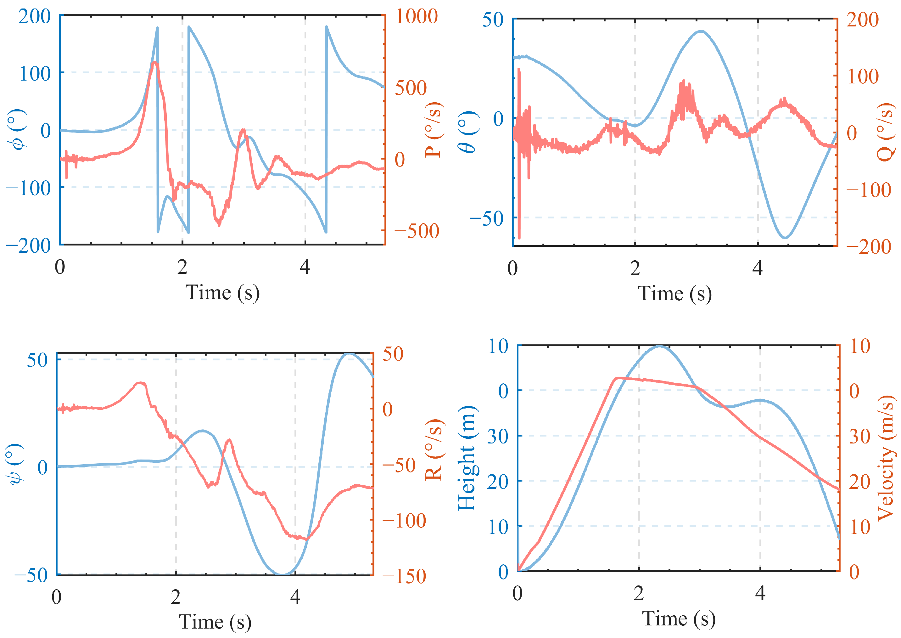
• We develop a comprehensive numerical simulation model for UAVs with rocket-assisted tube launch and wing deployment after launch. The model accounts for lumped disturbances, including model uncertainties and external disturbances. The accuracy of the model is thoroughly validated using data from an initial test flight.
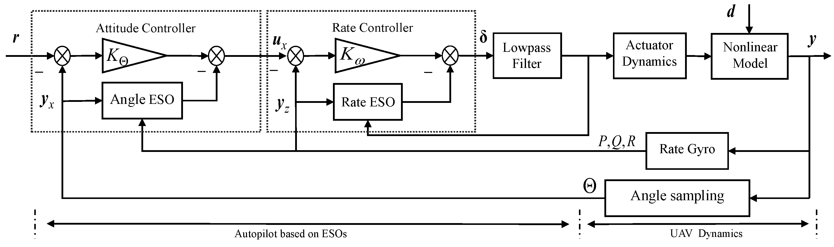
• An autopilot is designed for the UAVs based on the ESO disturbance observer. We prove the boundedness of the control error using Lyapunov stability theory and provide an upper bound estimate for the error.
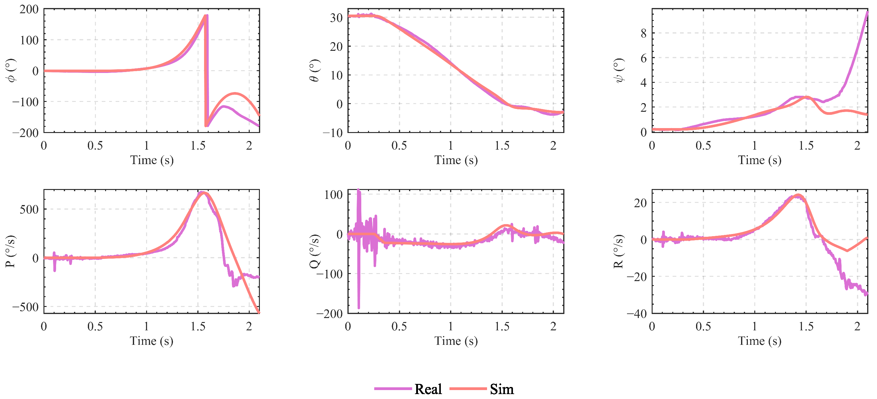
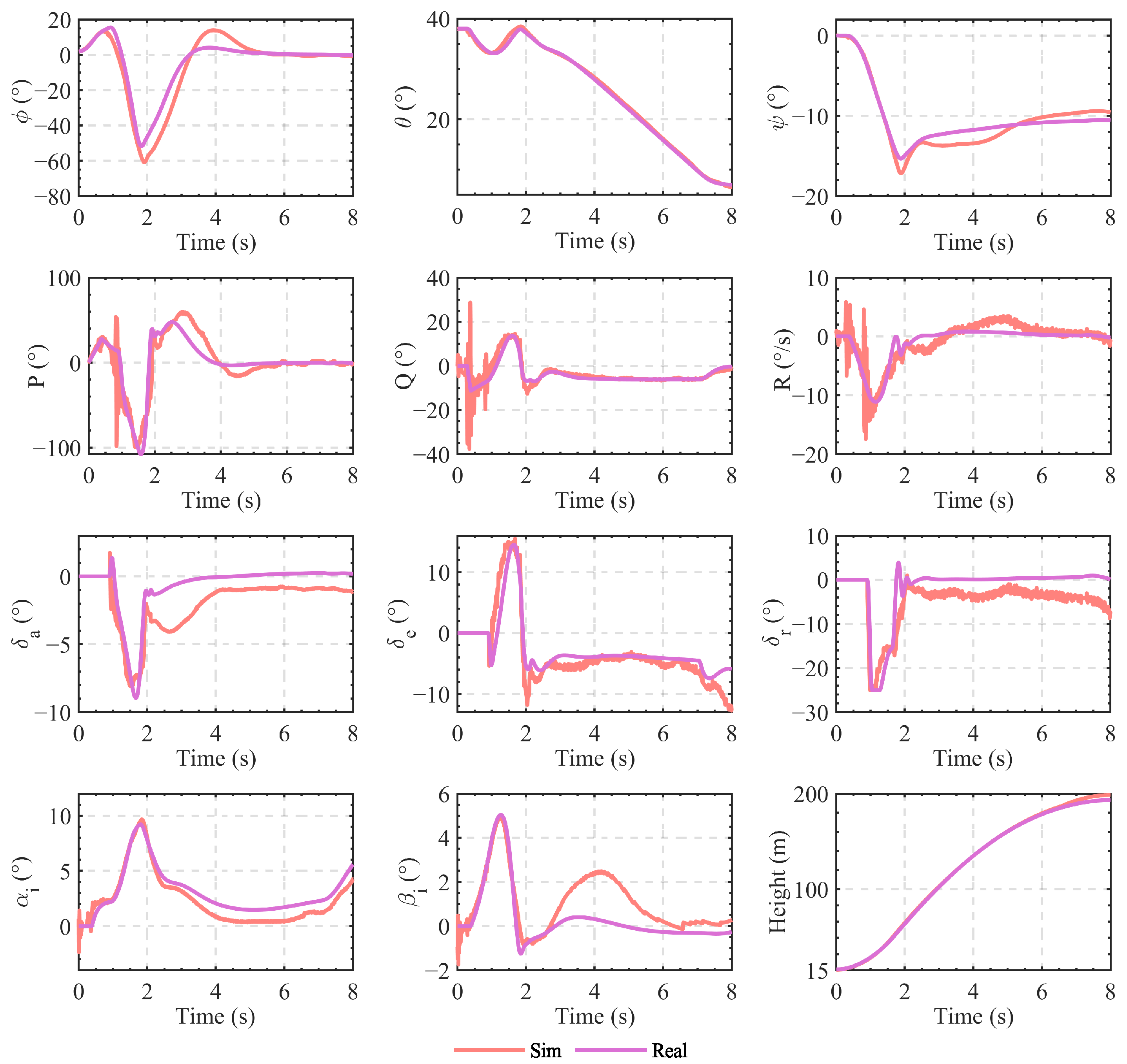
• Successful engineering implementation is demonstrated through comparative experiments and experimental data analysis, highlighting the strong robustness and anti-disturbance capabilities of the controller under high-disturbance launch conditions. This provides a widely applicable approach for implementing such UAVs with rocket-assisted tube launch and wing deployment after launch.

The remaining sections of the paper are structured as follows: Section 2 provides an analysis of flight instability sources based on previous test flight experiments, focusing on the main control challenges encountered during the launch process. In Section 3, we present a comprehensive six-degrees-of-freedom nonlinear model for rocket-assisted tube launch and wing deployment, including models for rocket propulsion, tube launch dynamics, wing deployment, and actuator dynamics. Section 4 proposes a robust control algorithm utilizing an ESO to ensure stability against disturbances during the launch process. Comparative experiments with traditional PID [33] methods under specific bias conditions and Monte Carlo simulations are presented in Section 5, along with new experimental flight data obtained using our proposed method. Finally, the key conclusions and future prospects are outlined in Section 6.

2. Problem Formulation

The launch method used in this paper is based on trainable launchers, which are pointed in the target’s direction together with the projectile [34]. As shown in Figure 2, the vehicle is initially set to a heading angle of 270°, indicating that it is oriented directly west. Additionally, the launch elevation is set to 30°, indicating the vehicle is launched at an angle 30° above horizontal. A booster rocket with a thrust-to-weight ratio of 6 and an effective boost time of approximately 1.7 s is used. The launch phase mainly involves the deployment of the tail fins and wings and booster separation. The actuation method is a programmed time sequence control (launch sequence). The program time for each stage in the first test flight experiment is shown in Figure 2.

In July 2023, we conducted a launch experiment following the timing sequence depicted in Figure 2. The launch site photos can be seen in Figure 3. According to the predesigned plan, once the main wings are fully deployed, the PID controller, as shown in Figure 4, has a stabilized pitch angle of approximately 7°, causing the UAV to climb up. The roll and heading angles were stabilized around 0° and 270°. However, the experimental results exceeded the expectations from the preliminary Monte Carlo simulations. Detailed data are presented in Figure 5.

The first experiment had a flight time of around 5 s, a maximum relative altitude of 25 m, and a maximum ground speed of 85.6 m/s.

At approximately 0.4 s, the amplitudes of the angular velocities along all three axes decreased. This indicates that the UAV successfully exited the launch tube, where the noise from factors such as combustion and friction was reduced. After exiting, the UAV experienced an unexpected rapid descent, with the pitch rate reaching a maximum of −30°/s, which we later analyzed to be caused by an additional pitching moment due to gravity. At 0.5 s, the V-tail deployment command was executed. Following this, the roll rate gradually increased, peaking at 600°/s, and the roll angle reached 180°, nearly putting the UAV in an inverted flight state. Once the wings were fully deployed, the controller began operating, bringing the roll angle back near 0°, although a roll rate oscillation of about 30°/s persisted. At the same time, in the pitch channel, the positive pitch moment from the lift after wing deployment was replaced by the negative pitch rate due to sensor lag. This caused a full deflection of the elevator in the negative direction, producing an additional positive pitch moment. As a result, the pitch angle increased from −2.4° to 44° between 2.1 and 3 s. At this point, the aerodynamic angle of attack of the UAV far exceeded the design point. The large angle of attack reduced the effective windward area of the V-tail, thereby diminishing aerodynamic stability. In this state, the control effectiveness of the ailerons and V-tail became unpredictable. Flight attitude remains uncontrolled at full-fin deflection, leading to a rapid decrease in speed and altitude. Consequently, the UAV crashed upon impact with the ground after 2 s. During the experiment, the flight became unstable due to attitude divergence mainly due to three factors. First, the angle of attack and sideslip angle in the second half of the flight far exceeded the design point, leading to instability. Second, the effective windward area of the V-tail becomes limited at a large angle of attack, making it prone to aerodynamic separation. This results in reduced control effectiveness or even adverse control effects. Third, the UAV studied in this paper utilizes a fuselage fuel tank, which is more than 20% of the weight when full of fuel. The dynamics of the center of gravity due to the violent shaking of the tank become unpredictable, thereby complicating the assessment of their impact on overall flight stability. Therefore, it is important to design the controller as much as possible to avoid large attitude states in flight due to uncertainty. An analysis of the experiment suggests the following issues in the launch phase:

• The short ejection time results in an insufficient initial velocity, causing the relatively heavy UAV to immediately enter the programmed turn after ejection. This reduces the aerodynamic stabilization effect and exacerbates the adverse influence of gravity on the pitch channel.
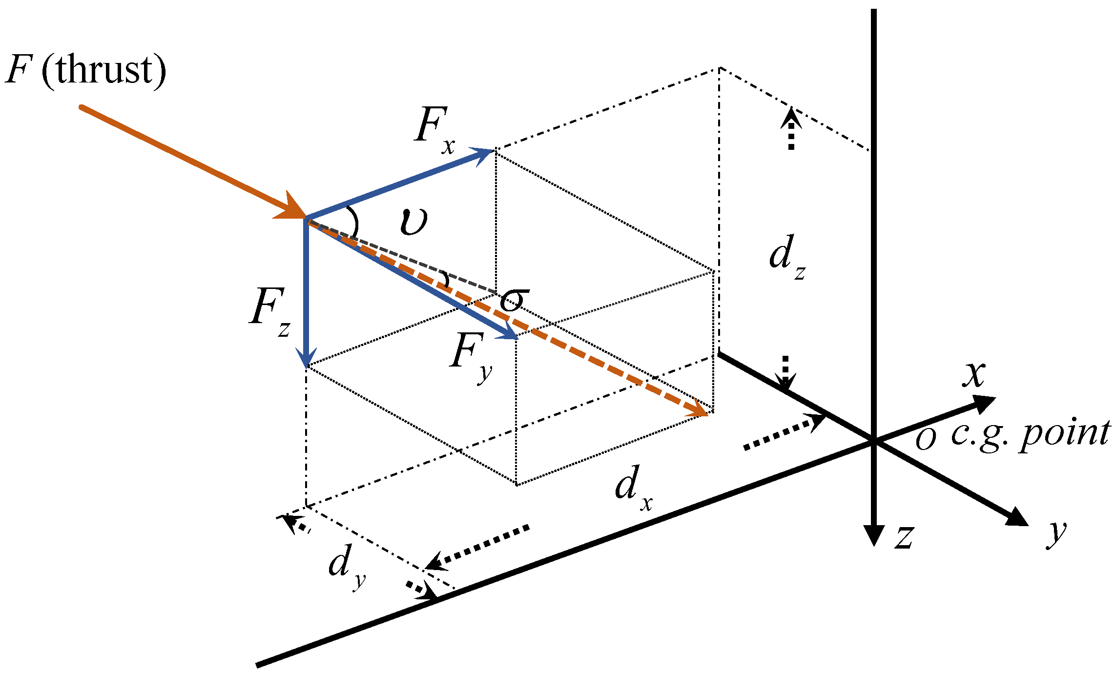
• Disturbances from installation errors and thrust deviations in the booster rocket can lead to side and normal forces, resulting in force and torque disturbances.
• Asynchronous tail fin deployment at high speeds (over 50 m/s) can induce additional aerodynamic moments, further deteriorating the roll rate.
• Abrupt changes in the center of gravity during wing deployment and booster separation cause variations in the aerodynamic forces, control forces, and stability.

The launch conditions are complex and highly nonlinear, especially at the critical points of ejection, tail fin deployment, wing deployment, and booster separation. Traditional control designs based on fixed coefficients have limited disturbance rejection capabilities. This paper focuses on establishing a reliable mathematical model based on flight test data, optimizing the launch solution, and designing a robust attitude control system using an extended state observer.

3. Materials and Methods

3.1. Reliable Mathematical Model

The mathematical model for UAVs is the basis of the control system design and simulations. Generally, UAV motion can be abstracted as a six-degrees-of-freedom rigid body motion, which can be described as a 12-state differential equation. The UAV is supported in the tube by two sets of sliders in the front and rear, with a 2–3 mm gap in the lateral and normal directions. The simplified mathematical model of the motion in the tube is given by

$$\left\{\begin{array}{c}\mathbf{a}=\left[\begin{array}{c}{F}_{roc}/m-gsin{\theta }_0\\ {\mathbf{0}}_{2\ast 1}\end{array}\right]\hfill \\ {\left[p,q,r\right]}^T={\mathbf{0}}_{3\ast 1}\hfill \end{array}\right.$$

(1)

where $\mathbf{a}$ denotes body-axis acceleration, $F_{roc}$ denotes the rocket thrust, g is the acceleration due to gravity, ${\theta }_0$ denotes the launch elevation, and $p,q,r$ are the UAV body angular rates. When the front slider is out of the tube but the rear slider is not, the UAV body rotates around the support point of the rear slider, and the main rotational driving force is gravity. A simplified rotation model is given by

$$\dot{q}=mgcos{\theta }_0\left(L_b-X_{cg}\right)+d_q$$

(2)

where $L_b$ and $X_{cg}$ denote the distance of the rear slider and the center of gravity in the geometric co-ordinate system of the airframe, respectively, and $d_q$ denotes the pitch perturbation.

Remark 1.

This analysis neglects factors such as friction support during the internal motion within the canister. However, in this 0.38 s stage, even with strong disturbances in the flight process, the changes in the state variables can be considered small perturbations within a finite time. The worst-case scenario at ejection is obtained by superimposing the disturbance extremes on the short-period variables at the moment of ejection. This ensures the stability of the subsequent flight.

According to reference [35], the rigid body dynamics model in air is described by the following six nonlinear ordinary differential equations:

$$\left\{\begin{array}{c}\dot{\varphi }=p+tan\theta (qsin\varphi +rcos\varphi )+d_{\varphi }\hfill \\ \dot{\theta }=qcos\varphi -rsin\varphi +d_{\theta }\hfill \\ \dot{\psi }={\displaystyle \frac{1}{cos\theta }}(qsin\varphi +rcos\varphi )+d\psi \hfill \\ \dot{p}=\overline{q}{S}_r[b_r{C}_l-(z_{cg}+\Delta z_{cg})C_y+(y_{cg}+\Delta y_{cg})C_z]/J_x\hfill \\ +(M_{xr}+M_{xp})/J_x+(J_y-J_x)qr/J_x+d_p\hfill \\ \dot{q}=\overline{q}{S}_r[c_r{C}_m-(x_{cg}+\Delta x_{cg})C_z+(z_{cg}+\Delta z_{cg})C_x]/J_y\hfill \\ +(M_{yr}+M_{yp})/J_y+(J_z-J_x)qr/J_y+d_q\hfill \\ \dot{r}=\overline{q}{S}_r[b_r{C}_n-(y_{cg}+\Delta y_{cg})C_x-(x_{cg}+\Delta x_{cg})C_y]/J_z\hfill \\ +(M_{zr}+M_{zp})/J_z+(J_x-J_y)pq/J_z+d_r\hfill \\ a_x=(\overline{q}{S}_r{C}_x+F_{xr}\left(t\right)+F_{xp}\left({\delta }_{eng}\right))/(m_0+\Delta m)-gsin\theta +d_{ax}\hfill \\ a_y=(\overline{q}{S}_r{C}_y+F_{yr}\left(t\right)+F_{yp}\left({\delta }_{eng}\right))/(m_0+\Delta m)+gcos\theta sin\varphi +d_{ay}\hfill \\ a_z=(\overline{q}{S}_r{C}_z+F_{zr}\left(t\right)+F_{zp}\left({\delta }_{eng}\right))/(m_0+\Delta m)+gcos\theta cos\varphi +d_{az}\hfill \end{array}\right.$$

(3)

where $\varphi ,\theta ,\psi$ denote the Euler angle, and $p,q,r$ are the body angular rates. $\overline{q}=0.5\rho V^2$ is the dynamic pressure, where $\rho$ is the air density. $d_i\left(i=\varphi ,\theta ,\psi ,p,q,r,a_x,a_{y,}{a}_z\right)$ represent external disturbances. V is the UAV velocity. $J_x=(1+{\eta }_x)J_{x0}$, $J_y=(1+{\eta }_y)J_{y0}$ and $J_z=(1+{\eta }_z)J_{z0}$ with ${\eta }_i,i=(x,y,z))$ are the parametric percentage errors of inertia. $x_{cg},y_{cg},z_{cg}$ indicate the center of gravity of the UAV, which has different values in different forms. $\Delta m,\Delta x_{cg},\Delta y_{cg},\Delta z_{cg}$ are the mass uncertainty and the center of gravity position uncertainties, respectively. $M_{ij}[(i=x,y,z),j=(r,p)]$ denotes the triaxial moment generated by the rocket thrust and the engine thrust. $F_{ij}[i=(x,y,z),j=(r,p)]$ denotes the fuselage axial component force generated by the rocket thrust and the engine thrust. Here, ${\delta }_{eng}\in \left[0,1\right]$ denotes the percentage of throttle for the turbojet engine. The schematic diagram of the additional torques generated by engine and rocket thrusts is depicted in Figure 6. By performing an orthogonal decomposition of the thrust forces and the distances from the thrust lines to the center of gravity, the following equations can be written:

$$\left\{\begin{array}{c}{F}_{xj}=F_j\cos ({\upsilon }_j\left)\cos \right({\sigma }_j)\hfill \\ F_{yj}=F_{j}sin\left({\sigma }_j\right)\hfill \\ F_{zj}=F_{j}sin\left({\upsilon }_j\right)cos\left({\sigma }_j\right)\hfill \\ M_{xj}=-F_{yj}{d}_{zj}+F_{zj}{d}_{yj}\hfill \\ M_{yj}=-F_{zj}{d}_{xj}+F_{xj}{d}_{zj}\hfill \\ M_{zj}=-F_{xj}{d}_{yj}+F_{yj}{d}_{xj}\hfill \end{array}\right.$$

(4)

where $\upsilon ,\sigma$ denote the angles between the thrust line and the planes $xoy,yoz$, respectively, and $d_{ij}[(i=x,y,z),j=(r,p)]$ denotes the distance from the thrust application point to the center of gravity. According to reference [36,37], in Equation (3), the dimensionless aerodynamic coefficients $C_i(i=x,y,z,l,m,n)$ depend on $V,\alpha ,\beta$ and the fin deflections $\delta ={\left[{\delta }_e,{\delta }_a,{\delta }_r\right]}^T$ and different folding states, which may be written as

$$\left\{\begin{array}{c}{C}_{\mathrm{l}}=(1+{\mu }_l)[C_l^0\left(\lambda \right)+C_l^{\beta }\left(\lambda \right)\beta +{\displaystyle \frac{b}{2V}}(C_l^r\left(\lambda \right)r+C_l^p\left(\lambda \right)p)]\hfill \\ +(1+{\xi }_l)(C_l^{{\delta }_a}\left(\lambda \right){\delta }_a+C_l^{{\delta }_r}\left(\lambda \right){\delta }_r)\hfill \\ C_m=(1+{\mu }_l)[C_m^0\left(\lambda \right)+C_m^{\alpha }\left(\lambda \right)\alpha +{\displaystyle \frac{c}{2V}}(C_m^q\left(\lambda \right)q+C_m^{\dot{\alpha }}\left(\lambda \right)\dot{\alpha })]\hfill \\ +(1+{\xi }_m)\left(C_l^{{\delta }_e}\left(\lambda \right){\delta }_e\right)\hfill \\ C_n=(1+{\mu }_n)[C_n^0\left(\lambda \right)+C_n^{\beta }\left(\lambda \right)\beta +{\displaystyle \frac{b}{2V}}(C_n^r\left(\lambda \right)r+C_n^p\left(\lambda \right)p)]\hfill \\ +(1+{\xi }_n)(C_n^{{\delta }_a}\left(\lambda \right){\delta }_a+C_n^{{\delta }_r}\left(\lambda \right){\delta }_r)\hfill \\ C_x=(1+{\mu }_x)[C_x^0\left(\lambda \right)+C_x^{\alpha }\left(\lambda \right)\alpha +{\displaystyle \frac{c}{2V}}(C_x^q\left(\lambda \right)q+C_x^{\dot{\alpha }}\left(\lambda \right)\dot{\alpha })]\hfill \\ +(1+{\xi }_x)\left(C_x^{{\delta }_a}\left(\lambda \right){\delta }_a\right)\hfill \\ C_y=(1+{\mu }_y)[C_y^0\left(\lambda \right)+C_y^{\alpha }\left(\lambda \right)\alpha +{\displaystyle \frac{b}{2V}}(C_y^r\left(\lambda \right)r+C_y^p\left(\lambda \right)p)]\hfill \\ +(1+{\xi }_y)\left(C_y^{{\delta }_e}\left(\lambda \right){\delta }_e\right)\hfill \\ C_z=(1+{\mu }_z)[C_z^0\left(\lambda \right)+C_z^{\alpha }\left(\lambda \right)\alpha +{\displaystyle \frac{c}{2V}}(C_z^q\left(\lambda \right)q+C_z^{\dot{\alpha }}\left(\lambda \right)\dot{\alpha })]\hfill \\ +(1+{\xi }_z)\left(C_z^{{\delta }_r}\left(\lambda \right){\delta }_r\right)\hfill \end{array}\right.$$

(5)

where $\lambda =[V,\alpha ,\beta ,\Lambda ]$ and $\Lambda$ denote the different folding states. $\alpha$ and $\beta$ are the angle of attack and the sideslip angle, respectively, which are unmeasurable. ${\delta }_e,{\delta }_a,{\delta }_r$ are the aileron deflection, elevator deflection, and rudder deflection, respectively. ${\mu }_i,{\xi }_j(i,j=x,y,z,l,m,n)$ are the aerodynamic uncertainties. $C_i^0(i=x,y,z,l,m,n)$ are dimensionless aerodynamic differential coefficients in the basic state and $C_i^{\beta },C_i^{\alpha }...$ are dimensionless aerodynamic differential derivative coefficients.

3.2. Model Reliability Verification

Before the first flight, we performed numerous Monte Carlo simulations, but the experimental results still exceeded expectations. This suggests that either the experimental conditions had unexpected variations or there were errors in the model. In fact, aerodynamic data and the six-degrees-of-freedom flight model are inherently based on actual physical models and possess a certain degree of maturity and reliability. The aerodynamic state point calculated in this paper is at 0.2 Ma. While this may not be as accurate for high Mach number scenarios, the aerodynamic data still hold significant reference values and should not significantly deviate from the actual situation. Prior to the experiment, we meticulously recorded the conditions, such as the center of gravity deviation, wind conditions at the time of flight, flight mass, and actual launch angle. Under the constraints of these conditions, we aim to reproduce the experiment as closely as possible to enhance the accuracy of the model and identify issues. As shown in Figure 7, the booster rocket exhibited a noticeable downward deviation. Unfortunately, this offset was immeasurable in this experiment.

By adjusting the deflection setting of the booster rocket and ensuring all recorded experimental measurement conditions were met, we obtained simulation results that closely matched the actual experimental data. We measured the center of gravity using the instrument shown in Figure 8. When compared with the ideal center of gravity point, we determined the center of gravity error to be $\Delta x_{cg}=0.005$ m, $\Delta y_{cg}=0.002$ m, and $\Delta z_{cg}=-0.001$ m, and the ground headwind was measured to be 4 m/s before the experiment. Simulations were conducted under these conditions and with $\upsilon =9\prime ,\sigma =-5\prime$, and the resulting data are shown in Figure 9.

Prior to 1.2 s, the flight states remain within the aerodynamic database envelope. The absolute value of $\theta ,\psi$ errors do not exceed 2°, and the $\psi$ errors do not exceed 10°. At 1.6 s, $\varphi$ exceeds 180°, and the maximum P exceeds 670°/s. This is approaching the edge of the aerodynamic database, which indicates the limits of the simulation’s accuracy. Although the simulation data exhibit a certain degree of similarity to the flight test data, simulation errors increase. Furthermore, the relatively small roll inertia amplifies the $\varphi$ error, with the maximum absolute value of the P error reaching 400°/s. The simulation results not only demonstrate that the model established in this paper has a certain degree of accuracy but also indicate that the deviation of the booster rocket is one of the main causes of the experimental failure.

4. Robust Observer and Controller Design

4.1. Scheme Iteration

During the first test, from 1 s to 1.6 s, the UAV exhibited a state in which the tail fins were fully deployed while the main wings remained undeployed and the booster rocket was still attached. In this stage, the uncontrolled tail fins led to an increased roll rate of 670°/s. Simultaneously, due to the nondeployment of the main wings, minimal lift was generated by the airframe, resulting in a forward center of gravity and a primarily nose-down moment produced by the tail fins. This caused a drop in pitch angle to −6°, further deteriorating the control window for subsequent controller activation. In order to address this issue, an optimized launch scheme was proposed that involves the earlier deployment of the main wings for enhanced attitude stabilization control. We advance the open tail to 0.8 s and the open winding to 0.9 s. This allows us to activate the attitude controller at 0.9 s, and boost separation can be advanced to 2.1 s.

The analysis above indicates that the aerodynamic changes during the deployment process are severe. Therefore, it is crucial to minimize the disturbances to the forces and moments caused by wing deployment and booster separation. On the one hand, we can control attitude by deploying the wing pairs as early as possible, and on the other hand, we can directly control the aerodynamic angle of attack and the sideslip angle to directly suppress strong aerodynamic changes. However, measuring the angle of attack presents certain challenges. When the flight speed decreases, the difference between the inertial angle of attack in the wind field and the actual angle of attack becomes significant, making direct feedback from the angle of attack unfeasible. By taking these factors into account, this paper adopts a segmented control approach. During phases 3 and 4, the control object is the inertial angle of attack. After phase 4, a control scheme based on the pitch angle is used, with the control objects being the pitch angle, roll angle, and inertial sideslip stabilization. The inertial angle of attack and inertial sideslip angle are given by

$$\left\{\begin{array}{c}sin{\beta }_i=cos\gamma \left[sin\varphi sin\theta cos\left(\psi -\chi \right)-cos\varphi sin\left(\psi -\chi \right)\right]\hfill \\ -sin\gamma sin\varphi cos\theta \hfill \\ sin{\alpha }_i=\left\{cos\gamma \left[cos\varphi sin\theta cos\left(\psi -\chi \right)+sin\varphi sin\left(\psi -\chi \right)\right]\right\}/cos{\beta }_i\hfill \\ -sin\gamma cos\varphi cos\theta /cos{\beta }_i\hfill \end{array}\right.$$

(6)

where $\gamma$ and $\chi$ denote the path and azimuth angles, respectively, which can be derived by converting the velocity measurements from the GPS. ${\alpha }_i$ and ${\beta }_i$ are the inertial angle of attack and inertial sideslip angle, respectively.

4.2. Disturbance Models

The nonlinear dynamic model in Equation (3) can be rewritten as

$$\left\{\begin{array}{c}\dot{\mathbf{\Theta }}=\mathbf{\Gamma }\left(\mathbf{\omega }\right)+{\mathbf{f}}_{\mathbf{\Theta }}\hfill \\ \dot{\mathbf{\omega }}=-{\mathbf{J}}^{-1}\mathbf{\omega }\otimes \mathit{J}\mathbf{\omega }+\mathbf{g}(\mathbf{J},\mathbf{\omega },\mathit{\delta })+{\mathbf{\tau }}_{\mathbf{e}}+{\mathbf{f}}_{\mathbf{\omega }}\hfill \\ \mathbf{y}=\mathbf{c}(\mathbf{\omega },\mathbf{\Theta },{\mathbf{f}}_{\mathbf{y}})\hfill \end{array}\right.$$

(7)

where $\mathbf{\Gamma },\mathbf{g},\mathbf{c}$ are twice continuously differentiable functions. Here, $\mathbf{\Theta }={\left[\varphi ,{\alpha }_0,{\beta }_0\right]}^T$, $\mathbf{\omega }={\left[p,q,r\right]}^T$ are the state vectors, $\mathit{\delta }={\left[{\delta }_a,{\delta }_e,{\delta }_r\right]}^T$ are the control input vectors, and ${\mathbf{y}}_{6\times 1}={[\mathbf{\Theta },\mathbf{\omega }]}^T$ is the controlled output vector that must track the control commands. ${\mathbf{J}}_{3\times 3}$ is the inertia matrix. $\mathbf{g}$ denotes the nonlinear control surface effectiveness, which is a function of the vehicle’s folding configuration, dynamic pressure, and angle of attack. ${\mathbf{\tau }}_{\mathbf{e}}={\mathbf{M}}_{\mathbf{r}}+{\mathbf{M}}_{\mathbf{p}}({\mathbf{\tau }}_{\mathbf{e}}\in {\mathbb{R}}^3)$ denotes moment interference from the boost and turbojet engines. ${\mathbf{f}}_{\mathbf{\Theta }},{\mathbf{f}}_{\mathbf{\omega }},{\mathbf{f}}_{\mathbf{y}}\in {\mathbb{R}}^3$ are the unmeasured disturbances (e.g., booster separation, mechanism deployment, sensor noise, and wind variations). Consequently, for a specified equilibrium point, the nonlinear model in Equation (7) is linearized and written in the following form:

$$\left\{\begin{array}{c}{\dot{\mathbf{x}}}_1={\mathbf{\Gamma }}^{\prime }{\mathbf{z}}_1+{\mathbf{d}}_1\hfill \\ {\dot{\mathbf{z}}}_1=\mathbf{A}{\mathbf{z}}_1+\mathbf{Bu}+{\mathbf{d}}_2\hfill \\ \mathbf{y}={\mathbf{C}}_1{\mathbf{x}}_1+{\mathbf{C}}_2{z}_1+\mathbf{D}{\mathbf{d}}_0\hfill \end{array}\right.$$

(8)

where ${\mathbf{x}}_1=\mathbf{\Theta }, {\mathbf{z}}_1=\mathbf{\omega }$, ${\mathbf{d}}_1={\mathbf{f}}_{\mathbf{\Theta }}, {\mathbf{d}}_0={\mathbf{f}}_{\mathbf{y}}$. ${\mathbf{B}}_{3\times 3}={\displaystyle \frac{\partial \mathbf{g}}{\partial \mathit{\delta }}}, {\mathbf{\Gamma }}^{\prime }={\displaystyle \frac{\partial \mathbf{\Gamma }}{\partial {\mathbf{z}}_1}}$, ${\mathbf{C}}_1={\displaystyle \frac{\partial \mathbf{c}}{\partial \mathbf{x}}}, {\mathbf{C}}_2={\displaystyle \frac{\partial \mathbf{c}}{\partial \mathbf{z}}},\mathbf{D}={\displaystyle \frac{\partial \mathbf{c}}{\partial {\mathbf{d}}_0}}$, with all Jacobian matrices of suitable dimensions evaluated. $\mathbf{A}\in {\mathbb{R}}^3\times {\mathbb{R}}^3$ is an angular velocity aerodynamic damping term. ${\mathbf{d}}_2=-{\mathbf{J}}^{-1}\mathbf{\omega }\otimes \mathit{J}\mathbf{\omega }+{{\mathit{f}}^{\prime }}_{\omega }+{\mathbf{\tau }}_{\mathbf{e}}$ denotes the total body torque disturbances, including the extra torque generated by neglecting the transformation of the co-ordinate system, the higher-order derivative terms of the fins effect function, the higher-order terms of the aerodynamic function, the extra torque generated by the turbojet engine and rocket boost, the mechanism deployment, and the boost drop disturbance torque.

Assumption 1. ${\mathbf{d}}_0,{\mathbf{d}}_1,{\mathbf{d}}_1$ denote uncertainties, including the model uncertainty, aerodynamic uncertainty, wing deployment uncertainty, and environmental uncertainty, which are unknown. From the results of the first test flight, ${\mathbf{\tau }}_{\mathbf{e}}\gg -{\mathbf{J}}^{-1}\mathbf{\omega }\otimes \mathit{J}\mathbf{\omega }+{{\mathit{f}}^{\prime }}_{\omega }$, ${\mathbf{\tau }}_{\mathbf{e}}$ makes up the majority of the uncertainty. We define $\eta =({\delta }_{{\tau }_e}-{\delta }_{trim})/{\delta }_{total}$, where ${\delta }_{{\tau }_e}$ denotes the trim fins with ${\tau }_e$ at different aerodynamic points, ${\delta }_{trim}$ denotes the inherent trim fins, and ${\delta }_{total}$ is all the available fins. Figure 10 shows $\eta$ values under extreme rocket boost conditions. The deviation of the trim fins does not exceed 35% of the total rudder deviation, so all the uncertainties can also be considered credible.

4.3. ESO-Based Controller Design

In the cascade attitude control framework, the ESO expands the system’s dimensions. The extended state represents the total disturbance of the system. In the angular dynamics Equation (8), the disturbance can be expressed as follows:

$$\left\{\begin{array}{c}\dot{{\mathbf{x}}_{\mathbf{1}}}={\mathbf{B}}_{x0}{\mathbf{z}}_1+{\mathbf{x}}_2\hfill \\ {\mathbf{x}}_2=({\mathbf{\Gamma }}^{\prime }-{\mathbf{B}}_{x0}){\mathbf{z}}_1+{\mathbf{d}}_1\hfill \end{array}\right.$$

(9)

where ${\mathbf{B}}_{x0}$ is the best available estimate of ${\mathbf{\Gamma }}^{\prime }$. In linear space, the angular dynamics Equation (9) can be further rewritten as

$$\left\{\begin{array}{c}\dot{\overline{\mathbf{x}}}={\overline{\mathbf{A}}}_x\overline{\mathbf{x}}+{\overline{\mathbf{B}}}_{x0}{\overline{\mathbf{u}}}_x+{\overline{\mathbf{K}}}_x{\mathbf{h}}_x\hfill \\ {\overline{\mathbf{y}}}_x={\overline{\mathbf{C}}}_x\overline{\mathbf{x}}+{\overline{\mathbf{D}}}_x{\mathbf{d}}_x\hfill \end{array}\right.$$

(10)

where $\overline{\mathbf{x}}={[{\mathbf{x}}_1,{\mathbf{x}}_2]}^T$, ${\mathbf{h}}_x={\dot{\mathbf{x}}}_2$, ${\overline{\mathbf{A}}}_x={\left[\begin{array}{cc}\mathbf{0}& {\mathbf{I}}_3\\ \mathbf{0}& \mathbf{0}\end{array}\right]}_{6\times 6}$, ${\overline{\mathbf{B}}}_{x0}={\left[\begin{array}{c}{\mathbf{B}}_{x0}\hfill \\ \mathbf{0}\hfill \end{array}\right]}_{6\times 3}$, and ${\overline{\mathbf{u}}}_x=\mathbf{\omega }$ is taken as the virtual input. The coupling terms and higher-order effects are lumped into ${\mathbf{d}}_1$. ${\overline{\mathbf{K}}}_x={\left[\begin{array}{c}\mathbf{0}\hfill \\ {\mathbf{I}}_3\hfill \end{array}\right]}_{6\times 3}$, ${\overline{\mathbf{C}}}_x={\left[{\mathbf{I}}_3,\mathbf{0}\right]}_{3\times 6}$, ${\overline{\mathbf{C}}}_x={\left[{\mathbf{I}}_3,\mathbf{0}\right]}_{3\times 6}$, ${\overline{\mathbf{D}}}_x={\mathbf{I}}_3$, ${\overline{\mathbf{y}}}_x$ denotes the angle output. ${\mathbf{d}}_x\in {\mathbb{R}}^3$ is measurement noise and other direct perturbations to the output ${\overline{\mathbf{y}}}_x$.

The state observer is constructed for the extended system (11):

$$\left\{\begin{array}{c}\dot{\widehat{\mathbf{x}}}={\overline{\mathbf{A}}}_x\widehat{\mathbf{x}}+{\overline{\mathbf{B}}}_{x0}{\overline{\mathbf{u}}}_x+{\mathbf{L}}_x({\overline{\mathbf{y}}}_x-{\widehat{\mathbf{y}}}_x)\hfill \\ \widehat{\mathbf{y}}={\overline{\mathbf{C}}}_x\widehat{\mathbf{x}}\hfill \end{array}\right.$$

(11)

where $\widehat{\mathbf{x}}={[{\widehat{\mathbf{x}}}_1,{\widehat{\mathbf{x}}}_2]}^T$, $\widehat{\mathbf{y}}$ are the estimated values of ${\overline{\mathbf{y}}}_x$ and $\overline{\mathbf{x}}$. ${\mathbf{L}}_x={\mathbf{I}}_6{\mathbf{\lambda }}_{6\times 1}$ is the observer gain matrix. The state estimation error vector is defined as ${\mathbf{e}}_{xo}=\overline{\mathbf{x}}-\widehat{\mathbf{x}}$. By combining Equations (10) and (11), we can obtain the error dynamics equation as follows:

$${\dot{\mathbf{e}}}_{xo}=\dot{\overline{\mathbf{x}}}-\dot{\widehat{\mathbf{x}}}=({\overline{\mathbf{A}}}_x-{\mathbf{L}}_x{\overline{\mathbf{C}}}_x){\mathbf{e}}_{xo}+{\overline{\mathbf{K}}}_x{\mathbf{h}}_x-{\overline{\mathbf{D}}}_x{\mathbf{d}}_x$$

(12)

From Equation (12), we can see that the observer error always converges if the observer’s gain matrix is sufficiently large. Without considering system disturbances, the observer converges exponentially. Moreover, the ESO does not require explicit expressions for the system’s state or input matrices. This allows unmodeled uncertainties, higher-order nonlinearities that are ignored in modeling, and external disturbances to be minimally considered. Hence, within the permissible bandwidth range, the ESO is insensitive to system parameters and nonlinear characteristics, providing the control system with strong robustness.

Remark 2.

A high gain in the ESO can increase the speed of error convergence. However, a high-gain observer can also reduce the closed-loop bandwidth. In practical situations, noise means that an excessively large gain matrix may amplify the noise, potentially causing the closed-loop system to become unstable. Therefore, it is important to strike a balance between the observer gain and the closed-loop performance to ensure the stability and robustness of the system.

Similarly, by expanding the angular velocity dynamics system (13), we have

$$\left\{\begin{array}{c}{\dot{\mathbf{z}}}_1={\mathit{B}}_{\delta 0}\mathit{\delta }+{\mathbf{z}}_2\hfill \\ {\mathbf{z}}_2=\mathbf{A}{\mathbf{z}}_1+({\mathit{B}}_{\delta }-{\mathit{B}}_{\delta 0})\mathit{\delta }+{\mathbf{d}}_2,\hfill \end{array}\right.$$

(13)

where ${\mathbf{B}}_{\delta 0}$ is the best available estimate of ${\mathit{B}}_{\delta }$. The dynamic equations of the entire system can be further written in the following form:

$$\left\{\begin{array}{c}\dot{\overline{\mathbf{z}}}={\overline{\mathbf{A}}}_{\mathbf{z}}\overline{\mathbf{z}}+{\overline{\mathit{B}}}_{\mathit{\delta }\mathbf{0}}\mathit{\delta }+{\overline{\mathbf{K}}}_{\mathbf{z}}{\mathbf{h}}_{\mathbf{z}}\hfill \\ {\overline{\mathbf{y}}}_{\mathbf{z}}={\overline{\mathbf{C}}}_{\mathbf{z}}\overline{\mathbf{z}}+{\overline{\mathbf{D}}}_{\mathbf{z}}{\mathbf{d}}_{\mathbf{z}}\hfill \end{array}\right.$$

(14)

where $\overline{\mathbf{z}}=\left[{\mathbf{z}}_1,{\mathbf{z}}_2\right]$, ${\mathbf{h}}_z={\dot{\mathbf{z}}}_2$, ${\overline{\mathbf{y}}}_z$ denote the angle rate output, ${\overline{\mathbf{A}}}_z={\left[\begin{array}{cc}\mathbf{0}& {\mathbf{I}}_{\mathbf{3}}\\ \mathbf{0}& \mathbf{0}\end{array}\right]}_{6\times 6}$, ${\overline{\mathit{B}}}_{\delta 0}={\left[\begin{array}{c}{\mathit{B}}_{\mathit{\delta }\mathbf{0}}\hfill \\ \mathbf{0}\hfill \end{array}\right]}_{\mathbf{6}\times \mathbf{3}}$, ${\overline{\mathbf{K}}}_z={\left[\begin{array}{c}\mathbf{0}\hfill \\ {\mathbf{I}}_{\mathbf{3}}\hfill \end{array}\right]}_{\mathbf{6}\times \mathbf{3}}$, ${\overline{\mathbf{C}}}_{\mathbf{z}}={\left[{\mathbf{I}}_{\mathbf{3}},\mathbf{0}\right]}_{\mathbf{3}\times \mathbf{6}}$, ${\overline{\mathbf{D}}}_{\mathbf{z}}={\mathbf{I}}_{\mathbf{3}}$ and ${\mathbf{d}}_z\in {\mathbb{R}}^3$ is direct perturbations to the angle rat output ${\overline{\mathbf{y}}}_z$. The angle rate ESO can be constructed as (15)

$$\left\{\begin{array}{c}\dot{\widehat{\mathbf{z}}}={\overline{\mathbf{A}}}_z\widehat{\mathbf{z}}+{\overline{\mathbf{B}}}_{\delta 0}\mathit{\delta }+{\mathbf{L}}_z({\overline{\mathbf{y}}}_z-{\widehat{\mathbf{y}}}_z)\hfill \\ {\widehat{\mathbf{y}}}_z={\overline{\mathbf{C}}}_z\widehat{\mathbf{z}}\hfill \end{array}\right.$$

(15)

where ${\mathbf{L}}_z={\mathbf{I}}_6{\mathrm{\Omega }}_{6\times 1}$ is the observer gain matrix. The observer error dynamics of the angle rate ESO are described as (16)

$${\dot{\mathbf{e}}}_{zo}=\dot{\overline{\mathbf{z}}}-\dot{\widehat{\mathbf{z}}}=({\overline{\mathbf{A}}}_z-{\mathbf{L}}_z{\overline{\mathbf{C}}}_z){\mathbf{e}}_{zo}+{\overline{\mathbf{K}}}_z{\mathbf{h}}_z-{\overline{\mathbf{D}}}_z{\mathbf{d}}_z$$

(16)

The overall system observer consists of an angle ESO and an angular velocity ESO. In the cascade system, the virtual input of the angle loop is designed as the command for the angular velocity loop. The attitude controller based on the cascade ESO can be summarized as follows:

$$\left\{\begin{array}{c}{\mathbf{u}}_x={\mathbf{K}}_{\mathbf{\Theta }}\left(\mathbf{r}-{\mathbf{y}}_x\right)-{\mathbf{B}}_{x0}^{-1}{\widehat{\mathbf{x}}}_2,\hfill \\ \mathit{\delta }={\mathbf{K}}_{\omega }\left({\mathbf{u}}_x-{\mathbf{y}}_z\right)-{\mathbf{B}}_{\delta 0}^{-1}{\widehat{\mathbf{z}}}_2,\hfill \end{array}\right.$$

(17)

where ${\mathbf{K}}_{\mathbf{\Theta }},{\mathbf{K}}_{\omega }$ are the autopilot angle error gain matrix and angular rate feedback gain matrix, respectively, and $\mathbf{r}$ is the reference input. The closed-loop autopilot’s control structure is depicted in Figure 11. Both the attitude and angular velocity controllers include a proportional term and a term for compensating the perturbations identified by the ESO. The control signal $\mathit{\delta }$ for the fins, generated by the cascade controller, is low-pass filtered to produce the final control signal, which is low-pass filtered to get the final output. This control framework is designed to compensate for the effects of the uncertainty perturbations, denoted as d, on the nonlinear model dynamics.

In the ESO-based controller proposed in this paper, we have the following adjustable parameters: ${\mathbf{L}}_x,{\mathbf{L}}_z,{\mathbf{K}}_{\mathbf{\Theta }},{\mathbf{K}}_{\omega },{\mathbf{B}}_{x0},{\mathbf{B}}_{\delta 0}$. The observer gains are designed in the linear observer form, as given in Ref. [38]. ${\mathbf{L}}_x=\left[2{\mathbf{\omega }}_x,{\mathbf{\omega }}_x^2\right], {\mathbf{L}}_z=\left[2{\mathbf{\omega }}_z,{\mathbf{\omega }}_z^2\right]$, where ${\mathbf{\omega }}_x=diag\left({\mathbf{\omega }}_{\varphi },{\mathbf{\omega }}_{\alpha },{\mathbf{\omega }}_{\beta }\right),{\mathbf{\omega }}_z=diag\left({\mathbf{\omega }}_p,{\mathbf{\omega }}_q,{\mathbf{\omega }}_r\right)$ are the observer’s bandwidth. The values of these gains are limited by factors such as the physical characteristics of the UAV, the sensor data acquisition frequency, and the control computation frequency. In this paper, a fixed observer gain method is adopted, defined by ${\mathbf{\omega }}_x=diag\left(2,2,2\right),{\mathbf{\omega }}_z=diag\left(5,5,3\right)$. The parameters ${\mathbf{B}}_{x0}$ and ${\mathbf{B}}_{\delta 0}$ are the best available estimates of ${\mathbf{\Gamma }}^{\prime }$ and ${\mathbf{B}}_{\delta }$. In the dynamic equation, they have a clear physical meaning. They are defined as

$$\left\{\begin{array}{c}{\mathbf{B}}_{x0}=diag\left(1,1,-1\right)\hfill \\ {\mathbf{B}}_{\delta 0}=diag\left({\displaystyle \frac{\overline{q}{S}_r{b}_r}{J_{x0}}}{C}_l^{{\delta }_a\ast }\left(\lambda \right),{\displaystyle \frac{\overline{q}{S}_r{c}_r}{J_{y0}}}{C}_m^{{\delta }_r\ast }\left(\lambda \right),{\displaystyle \frac{\overline{q}{S}_r{b}_r}{J_{z0}}}{C}_n^{{\delta }_r\ast }\left(\lambda \right)\right),\hfill \end{array}\right.$$

(18)

where $C_l^{{\delta }_a\ast },C_m^{{\delta }_r\ast },C_n^{{\delta }_r\ast }$ represent the dimensionless aerodynamic derivatives of the fins. These values do not need to be adjusted for different flight conditions and only need to be adjusted based on the flight altitude and velocity. The dynamic pressure, $\overline{q}$, can be calculated using the measurable airspeed and altitude. Therefore, for different operating points, the values are explicit and require no tuning. This means that only two parameters, ${\mathbf{K}}_{\Theta }=diag\left(k_{\varphi },k_{\alpha },k_{\beta }\right),{\mathbf{K}}_{\omega }=diag\left(k_p,k_q,k_r\right)$, are left to be tuned. They can be chosen in the following form:

$$\left\{\begin{array}{c}{\mathbf{K}}_{\Theta }={\mathbf{B}}_{x0}^{-1}diag\left(k_{\varphi 0},k_{\alpha 0},k_{\beta 0}\right),\hfill \\ {\mathbf{K}}_{\omega }={\displaystyle \frac{\overline{q}}{{\overline{q}}_0}}{\mathbf{B}}_{\delta 0}^{-1}diag\left(k_{p0},k_{q0},k_{r0}\right),\hfill \end{array}\right.$$

(19)

where $k_{\varphi 0},k_{\alpha 0},k_{\beta 0},k_{p0},k_{q0},k_{r0}$ could be constants at most operating points. ${\overline{q}}_0$ is the dynamic pressure at the operating point.

Remark 3.

The model described by Equation (3) is a highly nonlinear system. However, considering that the speed variation during flight is minimal, within the range of 55–75 m/s, the abrupt change in the center of gravity before and after booster separation causes differences in the model. Therefore, this paper presents designs for controllers for the states before and after booster separation to achieve stabilization control throughout the entire flight phase.

4.4. Closed-Loop Stability Analysis

For a reference input, $\mathbf{r}$, we can obtain the error between the system input and output, $\mathbf{e}=\left[\begin{array}{c}{\mathbf{e}}_{\mathbf{\Theta }}\hfill \\ {\mathbf{e}}_{\omega }\hfill \end{array}\right]={\left[\begin{array}{c}\mathbf{r}-{\overline{\mathbf{y}}}_x\hfill \\ {\mathbf{u}}_x-{\overline{\mathbf{y}}}_z\hfill \end{array}\right]}_{6\times 1}$. This results in the closed-loop system:

$$\left\{\begin{array}{c}{\dot{\mathbf{e}}}_{\Theta }=\dot{\mathbf{r}}-{\overline{\mathbf{D}}}_x{\dot{\mathbf{d}}}_x-{\overline{\mathbf{C}}}_x{\mathbf{B}}_{x0}{\mathbf{K}}_{\Theta }{\mathbf{e}}_{\Theta }-{\overline{\mathbf{C}}}_x\mathbf{Q}{\mathbf{e}}_{xo}\hfill \\ {\dot{\mathbf{e}}}_{\omega }={\dot{\mathbf{u}}}_x-{\overline{\mathbf{D}}}_z{\dot{\mathbf{d}}}_z-{\overline{\mathbf{C}}}_z{\mathbf{B}}_{z0}{\mathbf{K}}_{\omega }{\mathbf{e}}_{\omega }-{\overline{\mathbf{C}}}_z\mathbf{Q}{\mathbf{e}}_{zo}\hfill \end{array}\right.$$

(20)

where $\mathbf{Q}=\left[\mathbf{0},{\mathbf{I}}_{\mathbf{3}}\right]$, ${\dot{\mathbf{u}}}_x={\mathbf{K}}_{\Theta }\left(\dot{\mathbf{r}}-{\dot{\mathbf{y}}}_x\right)-{\mathbf{B}}_{x0}^{-1}{\dot{\widehat{\mathbf{x}}}}_2$. The error can be further written as (21)

$$\left\{\begin{array}{c}{\dot{\mathbf{e}}}_{\Theta }=-{\overline{\mathbf{C}}}_x{\mathbf{B}}_{x0}{\mathbf{K}}_{\Theta }{\mathbf{e}}_{\Theta }-{\overline{\mathbf{C}}}_x\mathbf{Q}{\mathbf{e}}_{xo}+\dot{\mathbf{r}}-{\overline{\mathbf{D}}}_x{\dot{\mathbf{d}}}_x\hfill \\ {\dot{\mathbf{e}}}_{\omega }=-{\overline{\mathbf{C}}}_z{\mathbf{B}}_{z0}{\mathbf{K}}_{\omega }{\mathbf{e}}_{\omega }-{\overline{\mathbf{C}}}_z\mathbf{Q}{\mathbf{e}}_{zo}-{\overline{\mathbf{C}}}_x{\mathbf{B}}_{x0}{\mathbf{K}}_{\Theta }^2{\mathbf{e}}_{\Theta }\hfill \\ -\left[{\mathbf{K}}_{\Theta }{\overline{\mathbf{C}}}_x\mathbf{Q}+{\mathbf{B}}_{x0}^{-1}\mathbf{Q}({\overline{\mathbf{A}}}_x-{\mathbf{L}}_x{\overline{\mathbf{C}}}_x)\right]{\mathbf{e}}_{xo}+\mathbf{N}\hfill \end{array}\right.$$

(21)

where $\mathbf{N}=-{\mathbf{B}}_{x0}^{-1}\mathbf{Q}\left({\overline{\mathbf{K}}}_z{\mathbf{h}}_z-{\overline{\mathbf{D}}}_z{\mathbf{d}}_z\right)+{\mathbf{K}}_{\Theta }\left(\dot{\mathbf{r}}-{\overline{\mathbf{D}}}_x{\dot{\mathbf{d}}}_x\right)-{\overline{\mathbf{D}}}_z{\dot{\mathbf{d}}}_z$. By rewriting Equation (21), we can further establish the following system (22)

$$\dot{\mathbf{e}}=\mathbf{Ae}+\mathbf{d}$$

(22)

where $\mathbf{e}={\left[\begin{array}{cccc}{\mathbf{e}}_{\Theta }& {\mathbf{e}}_{xo}& {\mathbf{e}}_{\omega }& {\mathbf{e}}_{zo}\end{array}\right]}^T$,

$\mathbf{d}={\left[\begin{array}{cccc}\dot{\mathbf{r}}-{\overline{\mathbf{D}}}_x{\dot{\mathbf{d}}}_x& {\overline{\mathbf{K}}}_x{\mathbf{h}}_x-{\overline{\mathbf{D}}}_x{\mathbf{d}}_x& \mathbf{N}& {\overline{\mathbf{K}}}_z{\mathbf{h}}_z-{\overline{\mathbf{D}}}_z{\mathbf{d}}_z\end{array}\right]}^T$, $\mathbf{A}={\left[\begin{array}{cccc}{\mathbf{A}}_1& {\mathbf{A}}_2& {\mathbf{A}}_3& {\mathbf{A}}_4\end{array}\right]}^T=\left[\begin{array}{cccc}-{\overline{\mathbf{C}}}_x{\mathbf{B}}_{x0}{\mathbf{K}}_{\Theta }& -{\overline{\mathbf{C}}}_x\mathbf{Q}& \mathbf{0}& \mathbf{0}\\ \mathbf{0}& {\overline{\mathbf{A}}}_x-{\mathbf{L}}_x{\overline{\mathbf{C}}}_x& \mathbf{0}& \mathbf{0}\\ -{\overline{\mathbf{C}}}_x{\mathbf{B}}_{x0}{\mathbf{K}}_{\Theta }^2& -{\mathbf{K}}_{\Theta }{\overline{\mathbf{C}}}_x\mathbf{Q}-{\mathbf{B}}_{x0}^{-1}\mathbf{Q}({\overline{\mathbf{A}}}_x-{\mathbf{L}}_x{\overline{\mathbf{C}}}_x)& -{\overline{\mathbf{C}}}_z{\mathbf{B}}_{z0}{\mathbf{K}}_{\omega }& -{\overline{\mathbf{C}}}_z\mathbf{Q}\\ \mathbf{0}& \mathbf{0}& \mathbf{0}& {\overline{\mathbf{A}}}_z-{\mathbf{L}}_z{\overline{\mathbf{C}}}_z\end{array}\right]$.

Theorem 1.

With Assumption 1 satisfied, the system in Equation (7) under the proposed control law in Equation (17) has input-to-state stability if $\dot{\mathbf{r}}$ and $\mathbf{d}$ are bounded and the observer gain ${\mathbf{L}}_x$, ${\mathbf{L}}_z$ in Equations (15) and (10) and the feedback control gains ${\mathbf{K}}_{\Theta }$ and ${\mathbf{K}}_{\omega }$ in Equation (17) are selected accordingly.

Proof .

The Gershgorin circle [39] theorem shows the following: Assume $\mathbf{A}$ is an $n\times n$ matrix with complex entries. For each $i=1,2,3\cdots n$, define $R_i={\displaystyle \sum _{j\ne i}}\left|a_{ij}\right|$, where $a_{ij}$ denotes the (i,j)-th entry of the matrix $\mathbf{A}$. Each eigenvalue $\lambda$ of $\mathbf{A}$ satisfies $D_i=\left\{{\lambda }_i\in \mathbb{C}:\left|{\lambda }_i-a_{ii}\right|\le R_i\right\}$. Thus, the eigenvalues of $\mathbf{A}$ are $\mathbf{\lambda }=\left\{{\mathbf{\lambda }}_1,{\mathbf{\lambda }}_2,{\mathbf{\lambda }}_3,{\mathbf{\lambda }}_4\right\}$. The values of ${\mathbf{\lambda }}_2,{\mathbf{\lambda }}_4$ are determined as ${\overline{\mathbf{A}}}_i-{\mathbf{L}}_i{\overline{\mathbf{C}}}_i(i=x,z)$. The gain matrix ${\mathbf{L}}_i$ is adjusted so that ${\mathbf{\lambda }}_2,{\mathbf{\lambda }}_4$ are distributed in negative values. Adjusting the feedback gain matrices ${\mathbf{K}}_{\Theta }$ and ${\mathbf{K}}_{\omega }$ so that $-{\overline{\mathbf{C}}}_x{\mathbf{B}}_{x0}{\mathbf{K}}_{\Theta }$, means that $-{\overline{\mathbf{C}}}_z{\mathbf{B}}_{z0}{\mathbf{K}}_{\omega }$ are the row representative elements and ${\mathbf{\lambda }}_1,{\mathbf{\lambda }}_3$ are negative as well. That means it is easy to make the matrix, $\mathbf{A}$, satisfy the Hurwitz stability criterion by adjusting the gain matrix ${\mathbf{K}}_{\Theta }$ and ${\mathbf{K}}_{\omega }$ of the feedback calibration and the observer bandwidth ${\mathbf{L}}_x$, ${\mathbf{L}}_z$.

According to the results in [40], we have the following:

• The result from Theorem 4.14: Let $f\left(x\right)$ be a local Lipschitz function defined over a domain $\mathbf{D}\subset R^n;0\in \mathbf{D}$ if the origin is an exponentially stable of $\dot{x}=f\left(x\right),\forall x\left(0\right)<r$. Then, there is a function, $V\left(x\right)$, that satisfies the following inequalities:

  $$\left\{\begin{array}{c}{c}_1{∥x∥}^2\le V\left(x\right)\le c_2{∥x∥}^2\hfill \\ \dot{V}\left(x\right)\le -c_3{∥x∥}^2\hfill \\ ∥{\displaystyle \frac{\partial V}{\partial x}}∥\le c_4∥x∥\hfill \end{array}\right.$$

  (23)

  where $c_1,c_2,c_3,c_4,r$ are positive constants.
• The result from Theorem 4.18: Let $D\subset R^n$ be a domain and $V:\left[0,\infty \right)\times D_0\to R$ be a function such that

  $$\left\{\begin{array}{cc}\hfill & {\alpha }_1\left({∥x∥}^2\right)\le V(t,x)\le {\alpha }_2{∥x∥}^2\hfill \\ \hfill & {\displaystyle \frac{\partial V}{\partial t}}+{\displaystyle \frac{\partial V}{\partial x}}f(t,x)\le -W_3\left(x\right),\forall ∥x∥\ge \mu >0\hfill \end{array}\right.$$

  (24)
  $\forall t\ge 0$ and $\forall x\in D$, where ${\alpha }_1,{\alpha }_2$ are class $\kappa$ functions and $W_3\left(x\right)$ is a continuous positives definite function. Take $r>0$ such that $B_r\subset D$ and suppose that $\mu <{\alpha }_2^{-1}\left({\alpha }_1\left(r\right)\right)$; then, there exists a class $\kappa$ function $\beta$, and for any initial state, $x\left(t_0\right)$, satisfying $\beta ={\alpha }_1^{-1}\left({\alpha }_2\left(\mu \right)\right)$, there exists a time, $T\ge 0$, such that the solution of the system satisfies

  $$\left\{\begin{array}{c}∥x\left(t\right)∥\le \beta (∥x\left(t_0\right)∥,t-t_0),\forall t_0\le t\le t_0+T\hfill \\ ∥x\left(t\right)∥\le {\alpha }_1^{-1}\left({\alpha }_2\left(\mu \right)\right),\forall t\ge t_0+T\hfill \end{array}\right.$$

  (25)

For linear systems, $\dot{\mathbf{e}}=\mathbf{Ae}$ has an exponentially stable equilibrium at the origin. As previously commented, by applying Theorem 4.14 [40], $V_0\left(\mathbf{e}\right)$ can be written as a continuously differentiable function such that

$$\left\{\begin{array}{c}{\lambda }_{min}\left(\mathbf{P}\right){∥\mathbf{e}∥}^2\le V_0\left(\mathbf{e}\right)\le {\lambda }_{max}\left(\mathbf{P}\right){∥\mathbf{e}∥}^2\hfill \\ {\dot{V}}_0\le c_3{∥\mathbf{e}∥}^2,∥{\displaystyle \frac{\partial V_0}{\partial e}}∥\le c_4∥\mathbf{e}∥\hfill \end{array}\right.\forall \mathbf{e}\in B_r=\left\{∥\mathbf{e}∥<r\right\}$$

(26)

where ${\lambda }_{min}(\cdot )$ and ${\lambda }_{max}(\cdot )$ denote the minimum and maximum eigenvalues of a matrix, with $\mathbf{P}$ satisfying the Lyapunov equation $\mathbf{PA}+{\mathbf{A}}^T\mathbf{P}=-\mathbf{Q}$. r, $c_3$, and $c_4$ are positive constants. $V_0\left(\mathbf{e}\right)$ is used to investigate the ultimate boundedness of the perturbed system $\dot{\mathbf{e}}=\mathbf{Ae}+\mathbf{d}$. Assume that $sup\left(∥\mathbf{d}∥\right)\le \delta ,\forall t\ge 0,e\in B_r$. $V:\left[0,\infty \right)\times D_0\to R$ is then defined so that

$$\begin{array}{cc}\hfill & \dot{V}\le -c_3{∥e∥}^2+∥{\displaystyle \frac{\partial V}{\partial e}}∥∥d∥\hfill \\ \hfill & \le -c_3{∥e∥}^2+c_4\delta ∥e∥\hfill \\ \hfill & =-(1-\theta )c_3{∥e∥}^2-\theta c_3{∥e∥}^2+c_4\delta ∥e∥\hfill \\ \hfill & \le -(1-\theta )c_3{∥e∥}^2,\forall ∥e∥\ge {\displaystyle \frac{\delta c_4}{\theta c_3}},\theta \in (0,1),\hfill \end{array}$$

(27)

where $\mu ={\displaystyle \frac{\delta c_4}{\theta c_3}}$. Theorem 4.18 [40] and Equation (26) are applied:

$\left\{\begin{array}{cc}& \mu <{\alpha }_2^{-1}\left({\alpha }_1\left(r\right)\right)\iff {\displaystyle \frac{\delta c_4}{\theta c_3}}<r\sqrt{{\displaystyle \frac{{\lambda }_{min}\left(P\right)}{{\lambda }_{max}\left(P\right)}}}\iff \delta <{\displaystyle \frac{c_3}{c_4}}\sqrt{{\displaystyle \frac{{\lambda }_{min}\left(P\right)}{{\lambda }_{max}\left(P\right)}}}\theta r\hfill \\ & b={\alpha }_1^{-1}\left({\alpha }_2\left(\mu \right)\right)\iff b=\mu \sqrt{{\displaystyle \frac{{\lambda }_{max}\left(P\right)}{{\lambda }_{min}\left(P\right)}}}\iff b={\displaystyle \frac{\delta c_3}{\theta c_4}}\sqrt{{\displaystyle \frac{{\lambda }_{max}\left(P\right)}{{\lambda }_{min}\left(P\right)}}}\hfill \end{array}\right.$. Therefore, for all $∥e\left(t_0\right)∥\le r\sqrt{{\displaystyle \frac{{\lambda }_{min}\left(P\right)}{{\lambda }_{max}\left(P\right)}}}$, the overall closed-loop system (19) is input-to-state stable to bounded ${\displaystyle \frac{\delta c_3}{\theta c_4}}\sqrt{{\displaystyle \frac{{\lambda }_{max}\left(P\right)}{{\lambda }_{min}\left(P\right)}}}$. □

Remark 4.

For system (8), linearization is always valid in the neighborhood around the operating point. If the initial disturbance does not exceed a certain threshold and the initial error range is within limits, the nonlinear system controlled by the controller will ultimately be uniformly bounded. The upper bound is determined by the gains of the controller and the observer.

5. Simulation Results

In practical engineering, the PID controller is the classic controller with representative significance. Therefore, a PID controller is selected as the baseline controller in this experiment. During the launch stage, the same controlled object is selected, and the PID controller parameters are determined through classical control theory.

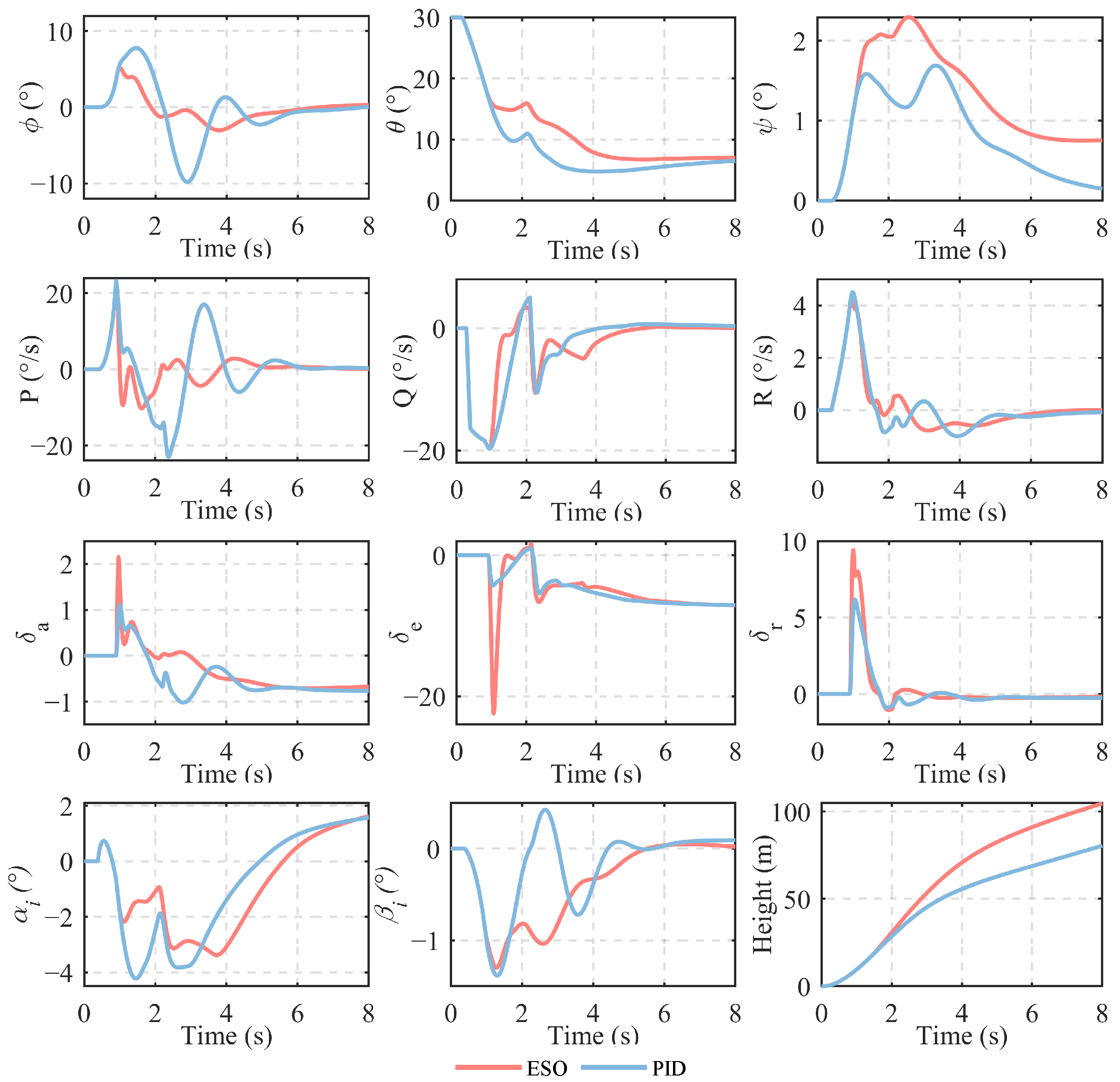
5.1. The Case of Fixed Operating Points

The dynamic performance of the controllers and the flight status in the time domain are evaluated under disturbance conditions. This analysis provides insights into the behavior and efficacy of the two control approaches when faced with external perturbations during flight. Before boost separation, we set the command $\left[{\alpha }_{icmd},{\varphi }_{cmd},{\beta }_{icmd}\right]=\left[-1,0,0\right]$. At an angle of attack of −1°, the longitudinal stability is high, and the angle of attack is close to the required 0° for separation. After separation, an attitude adjustment is performed, and the attitude command is maintained $\left[{\theta }_{cmd},{\varphi }_{cmd},{\beta }_{cmd}\right]=\left[7,0,0\right]$. The proposed ESO controller and PID simulation are compared in Figure 12.

Overall, both the PID and ESO-based controllers achieve stable flight, showing significant improvement compared to the first flight test. However, there are notable differences in their steady-state indices and dynamic performance. At the activation moment of 0.9 s, the control surfaces respond more sensitively to the ESO-based controller than the PID controller, resulting in smaller oscillations in the roll and sideslip angles. At 2.1 s, when the booster drops, the change in the center of gravity affects the three-axis angular velocities to varying degrees. The pitch and yaw rates show more pronounced changes under these deviations. The data indicate that the ESO-based controller responds more noticeably to disturbances at 2.1 s than the PID controller, maintaining a stable attitude after the rocket drops. In terms of steady-state accuracy, the ESO-based controller has a shorter adjustment time and faster convergence speed. We define $J=\underset{t_0}{\overset{t}{\int }}\left|R-S\right|dx$, where R denotes the command and S denotes the state variable. The results are listed in

Table 2. The control performance statistics under the two methods.

Notation	${\mathit{J}}_{{\mathit{\alpha }}_{\mathit{i}}}$ / ${\mathit{J}}_{\mathit{\theta }}$	${\mathit{J}}_{{\mathit{\beta }}_{\mathit{i}}}$	${\mathit{J}}_{\mathit{\varphi }}$	${\mathbf{J}}_{\mathbf{P}}$	${\mathbf{J}}_{\mathbf{Q}}$	${\mathbf{J}}_{\mathbf{R}}$
ESO	22.1120	47.0476	15.6231	132.4590	110.3229	25.8892
PID	45.4432	104.3141	12.8780	/	/	/

.

Table 2 shows that the instruction tracking error index of the ESO-based controller is smaller, with the longitudinal and roll channels being nearly half those of the PID controller. The simulation data indicate that the ESO-based controller has better control over the folding wings than the PID controller, with superior command tracking, robustness, and disturbance rejection.

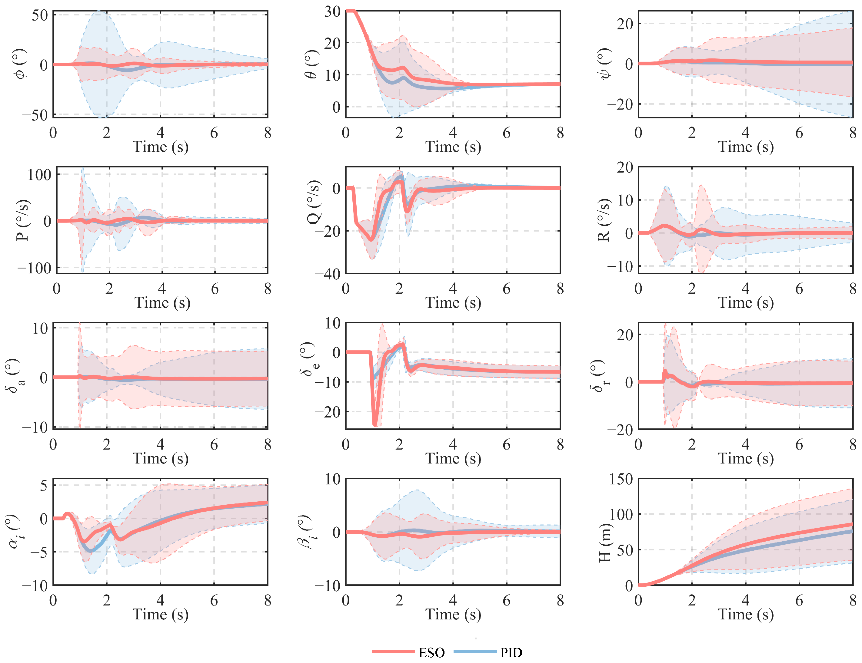
5.2. Monte Carlo Analysis

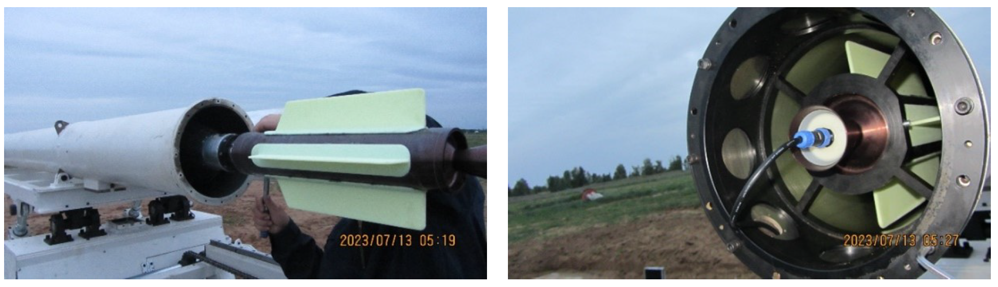
Both control schemes underwent 1000 Monte Carlo simulations during the launch phase, with environmental wind and uncertainties in the drag coefficient, the lift coefficient, the aerodynamic moment coefficient, the control surface effectiveness, atmospheric density, engine thrust, thrust line (deflection, eccentricity, and vehicle mass), center of gravity, and inertia taken into account. All uncertainties followed a Gaussian distribution. The wind model was a random process, with the wind components modeled as Gaussian distributions, with the local average wind speed as the mean and 3$\sigma$ of 20%. Random deviations in the lift coefficient, drag coefficient, aerodynamic moment coefficient, control surface effectiveness, air density, engine thrust, and mass also followed a zero-mean Gaussian distribution with 3$\sigma$ values of 10%, 20%, 10%, 20%, 5%, 10%, and 3 kg, respectively. Notably, the worst combination of these parameters could change the aerodynamic acceleration by 15%. Thrust deflection and eccentricity can cause force and moment disturbances, affecting guidance and attitude control systems. Their deviations were defined as normal distributions with means of −2° and 20 mm and 3$\sigma$ values of 10%. Crosswind and booster deflection deviations are the most likely causes of significant roll during flight. The results of the 1000 simulations are shown in Figure 13, with the shaded areas representing the 3$\sigma$ bounds during the simulation. In a steady state, both the PID and ESO controllers eventually converge, but the PID controller’s roll and sideslip channels converge more slowly. The clusters of the ESO are more concentrated, with the pitch angle lower bound improved by 4°. At 1.8 s, when the booster shuts down, the pitch angle lower bound improves by 6°. The roll angle variance decreases by 12.8°. In terms of altitude, the mean altitude of the ESO is higher by 10 m. The ESO controller is more energy efficient and superior to the PID controller.

6. Flight Tests

In August 2023, the second flight test was conducted with a launch angle of 38° and a headwind of 3 m/s. The total flight time was approximately 120 s. The results of the 1000 Monte Carlo simulations and the flight test data are shown in Figure 14. The red curve represents the mean of the Monte Carlo simulations, and the shaded area indicates the error band. The flight test data largely fall within the envelope of the preliminary simulations. Specifically, the pitch angle converges to 7° at 8 s. During launch, the maximum roll angle was −61° at 1.9 s, and the maximum roll rate was −100°/s at 1.4 s. The controller activated at 0.9 s, with the elevator reaching a maximum of 15°, the aileron 8°, and the rudder 25°, hitting the surface limits. The control performance was good, and the data show that the proposed controller can handle the complex conditions of the launch phase.

The test flight data still show a certain discrepancy with the nominal value of the pre-simulation. Some of the flight data are beyond the range of 3$\sigma$, which means that the boundaries of the bias settings are not accurately estimated. Alternatively, it might indicate that some other biases have not been accounted for. For this reason, we adjusted the bias size or added other biases according to the actual situation in order to make the simulation data as consistent as possible with the test flight data. The set of bias parameter settings that best fit the actual situation, making the simulation data most similar to the flight data, are shown in

Table 3. Bias parameter setting to best match the simulation data with the test flight data.

Notation	Wind	${\mathbf{X}}_{\mathbf{cg}}$	${\mathbf{Y}}_{\mathbf{cg}}$	${\mathbf{Z}}_{\mathbf{cg}}$	$\mathit{\upsilon }$
Bias	$-6$ m/s	0.1 m	4 mm	5 mm	2’
Notation	$\mathit{\sigma }$	${\mathit{C}}_{\mathit{m}}^{\mathit{\alpha }}$	${\mathit{C}}_{\mathit{n}}^{\mathit{\beta }}$	${\mathit{C}}_{\mathit{m}}^{{\mathit{\delta }}_{\mathit{e}}}$	${\mathit{\tau }}_{\mathit{\varphi }}$
Bias	3’	50%	70%	60%	35 $\mathrm{N}·\mathrm{m}$

.

${\tau }_{\varphi }$ denotes the unexpected roll moment in the launch phase. The simulation results are shown in Figure 15. Unexpectedly, most of these deviations are beyond the deviation range of the Monte Carlo simulation, in which the extra roll moment in the launch phase is 35 N · m. The pitch angle changes from 38° to 7° during the launch process, which results in the forward and backward movement of the fuel volume in the tank, causing a change in the center of gravity and making the forward center of gravity backward. The airborne firing of the turbojet engine is not considered in the pre-modeling. The uncertainty in the airborne ignition of the turbojet engine is also not considered in the pre-modeling, but the attitude is very controllable in the experiments and meets the accuracy requirements thanks to the proposed controller.

7. Conclusions

This paper proposes an innovative autopilot control framework and a comprehensive numerical simulation model tailored for UAVs with rocket-assisted tube launch and wing deployment. The crux of this framework is an ESO-based attitude controller, which provides real-time estimation of external disturbances, high-order aerodynamic coupling terms, and model uncertainties as generalized disturbances. The controller is theoretically proven to ensure the boundedness of control errors under unknown bounded disturbances, offering a robust solution for parameter tuning. This approach has been instrumental in enhancing the robustness and stability of the UAV during the critical launch phases. Comparative studies and Monte Carlo simulations showcased that the potential challenges of the launch phase have been successfully overcome by the strong robustness of the controller. Successful flight tests demonstrate that this method can replace traditional PID control and be widely accepted by engineering practitioners. Further work could introduce nonlinear features for different design points and incorporate nonlinear terms into the controller to enhance its adaptability further.

References

1. Zhang, Z.; Li, J.; Yang, Y.; Yang, C.; Mao, R. Research on Speed Scheme for Precise Attack of Miniature Loitering Munition. Math. Probl. Eng. 2020, 2020, 4963738. [Google Scholar] [CrossRef]
2. Yang, X.; Wang, T.; Liang, J.; Yao, G.; Liu, M. Survey on the Novel Hybrid Aquatic–Aerial Amphibious Aircraft: Aquatic Unmanned Aerial Vehicle (AquaUAV). Prog. Aerosp. Sci. 2015, 74, 131–151. [Google Scholar] [CrossRef]
3. Gao, L.; Zhu, Y.; Zang, X.; Zhang, J.; Chen, B.; Li, L.; Zhao, J. Dynamic Analysis and Experiment of Multiple Variable Sweep Wings on a Tandem-Wing MAV. Drones 2023, 7, 552. [Google Scholar] [CrossRef]
4. Chakravarthy, A.; Grant, D.T.; Lind, R. Time-Varying Dynamics of a Micro Air Vehicle with Variable-Sweep Morphing. J. Guid. Control. Dyn. 2012, 35, 890–903. [Google Scholar] [CrossRef]
5. Grant, D.T.; Abdulrahim, M.; Lind, R. Flight Dynamics of a Morphing Aircraft Utilizing Independent Multiple-Joint Wing Sweep. Int. J. Micro Air Veh. 2010, 2, 91–106. [Google Scholar] [CrossRef]
6. Seigler, T.M.; Neal, D.A.; Bae, J.S.; Inman, D.J. Modeling and Flight Control of Large-Scale Morphing Aircraft. J. Aircr. 2007, 44, 1077–1087. [Google Scholar] [CrossRef]
7. Liu, B.; Fang, Z.; Li, P.; Hao, C.C. Takeoff Analysis and Simulation of a Small Scaled UAV with a Rocket Booster. Adv. Mater. Res. 2011, 267, 674–682. [Google Scholar] [CrossRef]
8. Eymann, T.; Martel, J. Numerical investigation of launch dynamics for subscale aerial drone with Rocket Assisted Take-Off (RATO). In 2008 US Air Force T&E Days; American Institute of Aeronautics and Astronautics: Los Angeles, CA, USA, 2008; p. 1622. [Google Scholar] [CrossRef]
9. Martel, J.; Eymann, T. Numerical Investigation of Rail Influence on Initial Forces and Moments for Subscale Aerial Drone with Rocket Assisted Take-Off (RATO). In Proceedings of the 26th AIAA Applied Aerodynamics Conference, Honolulu, HI, USA, 18–21 August 2008. [Google Scholar] [CrossRef]
10. Martel, J.; Dudley, J. External Pitching Moment (EPM) Due to Turbine Engine Exhaust Impingement on Rocket Assisted Take Off (RATO) Bottle. In Proceedings of the 45th AIAA Aerospace Sciences Meeting and Exhibit, Reno, NV, USA, 8–11 January 2007. [Google Scholar] [CrossRef]
11. Voskuijl, M. Performance Analysis and Design of Loitering Munitions: A Comprehensive Technical Survey of Recent Developments. Def. Technol. 2022, 18, 325–343. [Google Scholar] [CrossRef]
12. Sayıl, A.; Erden, F.; Tüzün, A.; Baykara, B.; Aydemir, M. A Folding Wing System for Guided Ammunitions: Mechanism Design, Manufacturing and Real-Time Results with LQR, LQI, SMC and SOSMC. Aeronaut. J. 2024, 128, 788–811. [Google Scholar] [CrossRef]
13. Cheng, H.; Shi, Q.; Wang, H.; Shan, W.; Zeng, T. Flight Dynamics Modeling and Stability Analysis of a Tube-Launched Tandem Wing Aerial Vehicle during the Deploying Process. Proc. Inst. Mech. Eng. Part G J. Aerosp. Eng. 2022, 236, 262–280. [Google Scholar] [CrossRef]
14. Finigian, M.; Kavounas, P.A.; Ho, I.; Smith, C.C.; Witusik, A.; Hopwood, A.; Avent, C.; Ragasa, B.; Roth, B. Design and Flight Test of a Tube-Launched Unmanned Aerial Vehicle. Aerospace 2024, 11, 133. [Google Scholar] [CrossRef]
15. Li, C.Y.; Jing, W.X.; Gao, C.S. Adaptive Backstepping-Based Flight Control System Using Integral Filters. Aerosp. Sci. Technol. 2009, 13, 105–113. [Google Scholar] [CrossRef]
16. Lungu, R.; Lungu, M. Application of H 2 /H and Dynamic Inversion Techniques to Aircraft Landing Control. Aerosp. Sci. Technol. 2015, 46, 146–158. [Google Scholar] [CrossRef]
17. Doyle, J.; Glover, K.; Khargonekar, P.; Francis, B. State-Space Solutions to Standard H/Sub 2/ and H/Sub Infinity/Control Problems. IEEE Trans. Autom. Control 1989, 34, 831–847. [Google Scholar] [CrossRef]
18. Carter, L.H.; Shamma, J.S. Gain-Scheduled Bank-to-Turn Autopilot Design Using Linear Parameter Varying Transformations. J. Guid. Control. Dyn. 1996, 19, 1056–1063. [Google Scholar] [CrossRef]
19. Utkin, V. Variable Structure Systems with Sliding Modes. IEEE Trans. Autom. Control 1977, 22, 212–222. [Google Scholar] [CrossRef]
20. Moore, B. Principal Component Analysis in Linear Systems: Controllability, Observability, and Model Reduction. IEEE Trans. Autom. Control 1981, 26, 17–32. [Google Scholar] [CrossRef]
21. Altan, A.; Hacıoğlu, R. Model Predictive Control of Three-Axis Gimbal System Mounted on UAV for Real-Time Target Tracking under External Disturbances. Mech. Syst. Signal Process. 2020, 138, 106548. [Google Scholar] [CrossRef]
22. Chang, X.H.; Xiong, J.; Park, J.H. Fuzzy Robust Dynamic Output Feedback Control of Nonlinear Systems with Linear Fractional Parametric Uncertainties. Appl. Math. Comput. 2016, 291, 213–225. [Google Scholar] [CrossRef]
23. Jiang, B.; Li, B.; Zhou, W.; Lo, L.Y.; Chen, C.K.; Wen, C.Y. Neural Network Based Model Predictive Control for a Quadrotor UAV. Aerospace 2022, 9, 460. [Google Scholar] [CrossRef]
24. Altan, A.; Aslan, O.; Hacioglu, R. Real-Time Control Based on NARX Neural Network of Hexarotor UAV with Load Transporting System for Path Tracking. In Proceedings of the 2018 6th International Conference on Control Engineering & Information Technology (CEIT), Istanbul, Turkey, 25–27 October 2018; pp. 1–6. [Google Scholar] [CrossRef]
25. Altan, A.; Aslan, O.; Hacioglu, R. Model Reference Adaptive Control of Load Transporting System on Unmanned Aerial Vehicle. In Proceedings of the 2018 6th International Conference on Control Engineering & Information Technology (CEIT), Istanbul, Turkey, 25–27 October 2018; pp. 1–5. [Google Scholar] [CrossRef]
26. Shen, S.; Xu, J.; Xia, Q. A Fuzzy Backstepping Attitude Control Based on an Extended State Observer for a Tilt-Rotor UAV. Aerospace 2022, 9, 724. [Google Scholar] [CrossRef]
27. Shen, S.; Xu, J. Adaptive Neural Network-Based Active Disturbance Rejection Flight Control of an Unmanned Helicopter. Aerosp. Sci. Technol. 2021, 119, 107062. [Google Scholar] [CrossRef]
28. Talole, S.E.; Godbole, A.A.; Kolhe, J.P.; Phadke, S.B. Robust Roll Autopilot Design for Tactical Missiles. J. Guid. Control. Dyn. 2011, 34, 107–117. [Google Scholar] [CrossRef]
29. Yu, Y.; Wang, H.; Li, N.; Su, Z.; Wu, J. Automatic Carrier Landing System Based on Active Disturbance Rejection Control with a Novel Parameters Optimizer. Aerosp. Sci. Technol. 2017, 69, 149–160. [Google Scholar] [CrossRef]
30. Hu, Y.; Wu, M.; Zhao, K.; Song, J.; He, B. ADRC-Based Compound Control Strategy for Spacecraft Multi-Body Separation. Aerosp. Sci. Technol. 2023, 143, 108686. [Google Scholar] [CrossRef]
31. Ai, S.; Song, J.; Cai, G.; Zhao, K. Active Fault-Tolerant Control for Quadrotor UAV against Sensor Fault Diagnosed by the Auto Sequential Random Forest. Aerospace 2022, 9, 518. [Google Scholar] [CrossRef]
32. Zhu, W.; Wang, L.; Ren, Y.; Li, Y. Trajectory Tracking of UAVs Using Sigmoid Tracking Differentiator and Variable Gain Finite-Time Extended State Observer. Drones 2022, 6, 350. [Google Scholar] [CrossRef]
33. Åström, K.; Hägglund, T.; Hang, C.; Ho, W. Automatic Tuning and Adaptation for PID Controllers—A Survey. IFAC Proc. Vol. 1992, 25, 371–376. [Google Scholar] [CrossRef]
34. Głębocki, R.; Jacewicz, M. Sensitivity Analysis and Flight Tests Results for a Vertical Cold Launch Missile System. Aerospace 2020, 7, 168. [Google Scholar] [CrossRef]
35. Devaud, E.; Harcaut, J.P.; Siguerdidjane, H. Three-Axes Missile Autopilot Design: From Linear to Nonlinear Control Strategies. J. Guid. Control. Dyn. 2001, 24, 64–71. [Google Scholar] [CrossRef]
36. Lee, Y.; Kim, Y.; Moon, G.; Jun, B.E. Sliding-Mode-Based Missile-Integrated Attitude Control Schemes Considering Velocity Change. J. Guid. Control. Dyn. 2016, 39, 423–436. [Google Scholar] [CrossRef]
37. Lee, S.; Kim, Y.; Lee, Y.; Moon, G.; Jeon, B.E. Robust-Backstepping Missile Autopilot Design Considering Time-Varying Parameters and Uncertainty. IEEE Trans. Aerosp. Electron. Syst. 2020, 56, 4269–4287. [Google Scholar] [CrossRef]
38. Gao, Z. Scaling and Bandwidth-Parameterization Based Controller Tuning. In Proceedings of the 2003 American Control Conference, Denver, CO, USA, 4–6 June 2003; Volume 6, pp. 4989–4996. [Google Scholar] [CrossRef]
39. Chien, M.T.; Fang, S.T.; Su, Y.X. A Generalization of Gershorin Circles. Appl. Comput. Math. 2016, 15, 106–111. [Google Scholar]
40. Khalil, H.K. Nonlinear Systems, 3rd ed.; Prentice Hall: Upper Saddle River, NJ, USA, 2002. [Google Scholar]
Figure 1. The UAV configuration and co-ordinate system.
Drones 08 00363 g001
Figure 2. UAV launch scheme in the first test.
Drones 08 00363 g002
Figure 3. The stages of the first flight test.
Drones 08 00363 g003
Figure 4. Block diagram of the first flight’s autopilot.
Drones 08 00363 g004
Figure 5. Evolution of the state variables in the first flight test.
Drones 08 00363 g005
Figure 6. Diagram of additional torques due to thrust uncertainty.
Drones 08 00363 g006
Figure 7. Booster rocket state in the first flight test.
Drones 08 00363 g007
Figure 8. Center of mass measuring instrument.
Drones 08 00363 g008
Figure 9. A comparison of the first test and repeat simulation.
Drones 08 00363 g009
Figure 10. The fin deflection increment distribution under extreme flight conditions.
Drones 08 00363 g010
Figure 11. The control structure of the closed-loop autopilot.
Drones 08 00363 g011
Figure 12. Conditions were reproduced for the first test state and control variable profiles.
Drones 08 00363 g012
Figure 13. A comparative analysis of the control errors of the two methodologies.
Drones 08 00363 g013
Figure 14. Comparison of simulation results from 1000 Monte Carlo runs and the second flight test.
Drones 08 00363 g014
Figure 15. Comparative plots of the second flight test data and recreated simulation results.
Drones 08 00363 g015