Enhancing Mission Planning of Large-Scale UAV Swarms with Ensemble Predictive Model

Abstract

Target assignment and trajectory planning are two crucial components of mission planning for unmanned aerial vehicle (UAV) swarms. In large-scale missions, the significance of planning efficiency becomes more pronounced. However, existing planning algorithms based on evolutionary computation and swarm intelligence face formidable challenges in terms of both efficiency and effectiveness. Additionally, the extensive trajectory planning involved is a significant factor affecting efficiency. Therefore, this paper proposes a dedicated method for large-scale mission planning. Firstly, to avoid extensive trajectory planning operations, this paper suggests utilizing a machine learning algorithm to establish a predictive model of trajectory length. To ensure predictive accuracy, an ensemble algorithm based on Gaussian process regression (GPR) is proposed. Secondly, to ensure the efficiency and effectiveness of target assignments in large-scale missions, this paper draws inspiration from a greedy search and proposes a simple yet effective target assignment algorithm. This algorithm can effectively handle a large number of decision variables and constraints involved in large-scale missions. Finally, we validated the effectiveness of the proposed method through 15 simulated missions of different scales. Among the 10 medium- to large-scale missions, our method achieved the best results in 9 of them, demonstrating the competitive advantage of our method in large-scale missions. Comparative results demonstrate the advantage of the proposed methods from both prediction and mission planning perspectives.

1. Introduction

Mission planning is a critical component in ensuring the efficiency of a UAV swarm. [1,2,3]. In scenarios involving multiple targets and threat sources, the role of mission planning includes allocating suitable targets to UAVs (referred to as target assignment, TA) and planning trajectories to reach those targets (referred to as trajectory planning, TP). Clearly, TA and TP are two interdependent sub-problems within mission planning [4,5,6]. In TA, trajectory length is a key objective function, whose calculation requires TP. On the other hand, TP relies on TA to provide the starting and ending points for each trajectory. As a result, a competent mission planning method needs to address TA and TP simultaneously, although many studies have treated them separately [7,8,9,10].

In [11], the problem of coordinated target assignment and intercept is addressed for UAV systems. Three components, namely target manager, path planning, and intercept manager, are developed to work together to generate waypoint paths for each UAV. The target manager employs satisficing decision theory [12] to address the target assignment problem, where four typical objectives are considered. The path planner that employs a k-best paths graph search [13] of a Voronoi diagram aims to derive a set of waypoints and commanded velocity for each UAV. In [14], a four-stage method is proposed to address the problem of multi-target assignment and path planning for a group of UVAs. In the first two stages, a feasible set of path elements is generated on the Voronoi graph, through which short paths can be identified. In the third stage, a semi-greedy heuristic is used to divide tasks among UAVs equally. The initial assignment is finally refined using spatially constrained exchange of sub-paths in the fourth stage. In [15], the cooperation of task assignment and path planning of multiple UAVs for missions of suppression of enemy air defense is addressed. Timing constraints for simultaneous attacks and multiple consecutive tasks with specified time delays are applied in advanced missions. To find a feasible assignment that satisfies the time constraints, multiple candidate paths of various lengths are generated for each pair of UAVs and targets. The final assignment result is derived by the genetic algorithm. With the extra consideration of possible collisions between UAVs, the cooperation of target assignment and path planning with timing constraints is also addressed in [7]. The rationale of the proposed method is similar to that proposed in [15]. In [16,17], a hierarchical fuzzy logic controller is proposed to solve the assignment problem, ensuring that each team of UAVs is assigned to a unique target. Algorithm particle swarm optimization is then employed to solve the optimization problem formulated from path planning. To improve the performance in dynamic environments in terms of multi-UAV target assignment and path planning, a multi-agent reinforcement learning algorithm named multi-agent deep deterministic policy gradient is employed [18]. The reward structure is designed by combining travel distance and collision avoidance, which are key elements in target assignment and path planning, respectively.

Although these mission planning methods have taken into account both TA and TP, yielding promising experimental results, they have primarily focused on smaller-scale mission scenarios, raising concerns about their applications in large-scale missions. With the escalation of mission complexity, there is a discernible surge in the number of targets and threat sources, consequently driving the expansion of the UAV swarm scale and posing significant challenges to mission planning. First and foremost, as the mission scale increases, the number of decision variables in TA grows, resulting in an exponential expansion of the solution space. This significantly increases the difficulty of searching for the optimal solution. Furthermore, the number of constraints in TA also increases with the growth of mission scale. This leads to a significant reduction in the proportion of feasible solutions. Considering that TA falls under the category of discrete optimization, the difficulty of finding the optimal solution is further compounded.

Another common drawback of these mission planning methods is that they only consider static mission scenarios, which poses challenges to their computational efficiency in dynamic environments. While the reinforcement learning algorithm presented in [18] demonstrates good adaptability to dynamic environments, its training burden may limit its application in large-scale missions. In addition, its generalization performance in new scenarios still faces challenges. It is widely acknowledged that uncertainty is one of the prominent characteristics of complex missions. When mission information suddenly changes, the original planning result may lead to mission failure or significant performance degradation, necessitating mission replanning. Against this background, the computational efficiency of the mission planning method becomes crucial, as low efficiency can potentially result in mission failure.

Taking into account the shortcomings of existing mission planning methods, this paper proposes an efficient mission planning approach suitable for large-scale missions. Firstly, to address the challenges posed by a large number of decision variables and constraints in TA, this paper presents a simple yet effective greedy search algorithm tailored to the mission characteristics of UAVs. The computational complexity of this algorithm is linearly related to the number of decision variables, making it suitable for application in large-scale missions. While this algorithm cannot guarantee finding the globally optimal solution, it exhibits a clear advantage in terms of solution optimality compared to swarm intelligence algorithms in large-scale missions. Additionally, to further enhance the efficiency of mission planning, we propose a machine learning-based prediction model to estimate the trajectory length instead of employing actual TP algorithms. To the best of our knowledge, the introduction of machine learning algorithms for trajectory length prediction has not been considered by existing mission planning methods. It is important to note that the trajectory length mentioned here serves as an objective function for TA, and the actual trajectory generation still requires specific TP algorithms in subsequent steps. In the case of dynamic environments and new scenarios in large-scale missions, the proposed planning method is expected to provide an effective replanning result fast enough to assure the success of the mission.

In summary, the contribution of this paper is twofold:

(1)

By leveraging the greedy search, we propose a UAV swarm target assignment algorithm suitable for large-scale missions. This algorithm demonstrates a balanced combination of solving efficiency and effectiveness in large-scale missions.

(2)

We propose a machine learning-based approach to predict trajectory length, aiming to ensure the efficiency of the mission planning algorithm during replanning and, consequently, enhance mission success rates.

The remainder of this paper is organized as follows. In Section 2, we formulate the problem of mission planning into a constrained optimization problem. Details of the proposed mission planning method will be presented in Section 3. In Section 4, multiple simulated missions are generated to verify the proposed method. Finally, Section 5 draws some conclusions.

2. Problem Formulation

This paper focuses on the mission planning problem for UAV swarms. The mission requires that each target be visited by at least one UAV, and each UAV can only visit one target. Therefore, it is typically assumed that the number of available UAVs exceeds the number of targets. In addition, the information regarding targets, threats, and UAVs is known prior to mission planning. To achieve maximum mission utility, TA typically involves optimizing the total trajectory length, total trajectory safety, and total target value.

Given a trajectory t, the trajectory length can be represented as:

$$L\left(t\right)={\displaystyle \sum _{i=1}^{K-1}\sqrt{{\left(x_{i+1}-x_i\right)}^2+{\left(y_{i+1}-y_i\right)}^2}}$$

(1)

where K denotes the number of waypoints, and $\left(x_i,y_i\right)$ represent the coordinates of waypoint i in the trajectory t.

In general, the benefits generated by UAVs visiting different targets are typically different, often determined by the nature of the targets. In this paper, the value of a target is used to define the benefit of a trajectory. Consequently, the benefit B(t) of trajectory t is determined by the value of the target to which it is assigned.

In many studies, the safety of a trajectory is commonly represented by the distance between threat sources and the trajectory, where a greater distance indicates higher safety. However, in this paper, due to the predetermined threat regions, the trajectory planning algorithm can easily find a trajectory that balances both the length and avoidance of threat regions. In other words, no trajectory for any UAV to any target will enter a threat region. Therefore, this paper considers that there is no need to further consider the safety of trajectories during TA. It is worth emphasizing that we are not stating that safety is unimportant. Rather, due to the complete resolution of safety concerns during TP, there is no need to further consider it in TA.

By combining these three factors, we obtain a comprehensive objective function.

$$f\left(t\right)=\alpha \cdot L\left(t\right)-\left(1-\alpha \right)\cdot B\left(t\right)$$

(2)

where $\alpha \in \left(\mathrm{0,1}\right)$ is the parameter representing the weight of the length for trajectory t. $N_u$ and $N_t$ represent the number of UAVs and targets, respectively. Note that values of length and benefit are normalized before combination. Then, the objective function of TA is formulated as:

$$F={\displaystyle \sum _{i=1}^{N_u}{\displaystyle \sum _{j=1}^{N_t}\left[\alpha \cdot L\left(t_{ij}\right)-\left(1-\alpha \right)\cdot B\left(t_{ij}\right)\right]\cdot x_{ij}}}$$

(3)

where $x_{ij}$ denotes the decision variable. Its value is equal to 1 if the i-th UAV visits the j-th target and 0 if it does not. $t_{ij}$ denotes the corresponding trajectory. Finally, the problem of TA can be described as:

$$\begin{array}{ll}\hfill \min & F\hfill \\ \hfill s.t.& {\displaystyle \sum _{j=1}^{N_t}{x}_{ij}}=1, 1\le i\le N_u\hfill \\ & {\displaystyle \sum _{j=1}^{N_u}{x}_{ij}}\ge 1, 1\le i\le N_t\hfill \end{array}$$

(4)

Given a starting point, an endpoint, and threat regions, the objective of trajectory planning is to find the shortest trajectory from the starting point to the endpoint while ensuring avoidance of the threat regions [19]. Therefore, prior to TA, it is necessary to utilize a designated TP algorithm to obtain the trajectory for each UAV to reach each target. Only then can the specific trajectory length be calculated. The purpose of TA is to achieve the maximization of overall UAV swarm performance or efficiency.

3. Methodology

In solving the problem of mission planning for large-scale tasks, two key factors affect efficiency: generating trajectories for each UAV to each target and searching for the optimal solution for TA. While the former can be alleviated using efficient TP algorithms, its effectiveness may still be limited when dealing with large-scale tasks. On the other hand, the latter can only be addressed by proposing an efficient TA algorithm.

3.1. Ensemble Predictive Model of Trajectory Length

In TA, what we need is the length of each trajectory rather than the specific trajectories themselves. Therefore, generating all trajectories using a TP algorithm would be unnecessary and inefficient. The most straightforward solution is to use the Euclidean distance between the UAV and the target as the trajectory length between them. However, this approach can lead to significant estimation bias in large-scale complex missions, affecting the optimality of the solution of TA. To this end, this paper proposes using a machine learning algorithm to establish a predictive model of trajectory length. Establishing an accurate predictive model requires addressing two key issues: determining appropriate data features and utilizing an effective machine learning algorithm [20].

3.1.1. Feature Extraction

While estimating the trajectory length using the Euclidean distance may not be suitable, this distance is indeed the most important data feature for predicting the true trajectory length. This is because all trajectory planning algorithms strive to search for the shortest trajectory, and this distance represents the shortest distance in the absence of threat sources. For ease of reference, we define the straight line between each UAV and its target as the baseline of the corresponding trajectory. It is easy to understand that the presence of threat sources is the reason for the deviation introduced when using the baseline. When the baseline intersects a threat region, the true trajectory length experiences an increment. Therefore, we define the threat sources that intersect with the baseline as dominant threats. Clearly, the number and threat radius of dominant threats will have an impact on the increment. The greater the number or larger the radius, the larger the increment will be. Considering different scenarios where the number of dominant threats may vary, it is more appropriate to use the average value of threat radius. Nevertheless, for identical dominant threats, the resulting increment can vary based on the specific intersection points with the baseline. To account for this, we propose adjusting each threat radius with a coefficient.

$$\eta ={\displaystyle \frac{r-d}{r}}=1-{\displaystyle \frac{d}{r}}$$

(5)

where r and d represent the threat radius and the distance from the threat to the baseline, respectively.

In summary, we have concluded three data features, i.e., the length of baseline $l_B$, the number of dominant threats $n_{DT}$, and the adjusted averaging threat radius of dominant threats $r_{AR}$.

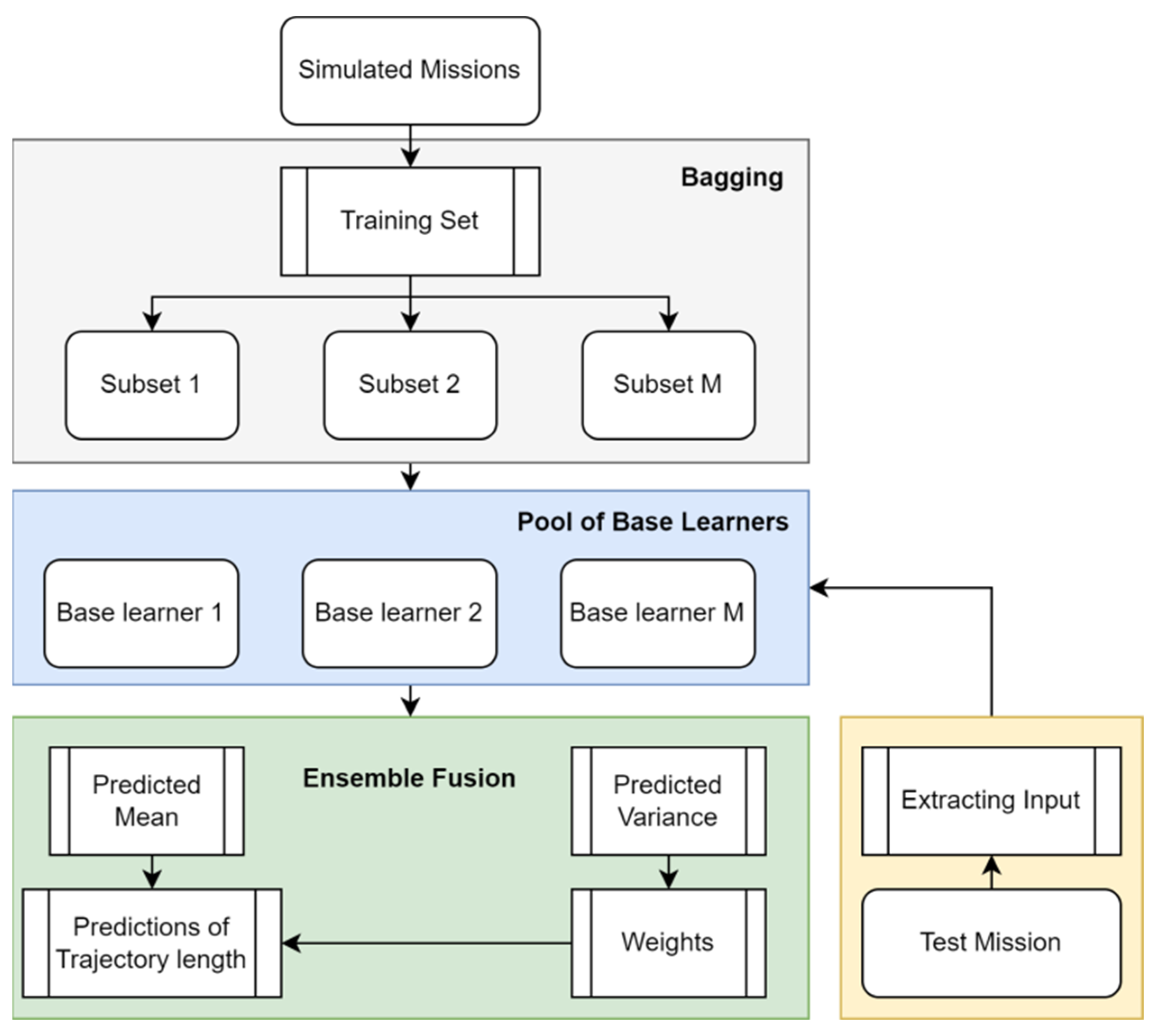
3.1.2. Ensemble of GPR

The prediction of trajectory length fundamentally falls within the domain of regression in machine learning. To ensure predictive performance, this paper proposes constructing an ensemble predictive model due to the excellent performance of ensemble learning in machine learning [21,22]. Using Bayesian nonparametric models as base learners in an ensemble model offers two advantages. First, the predicted results have statistical interpretations, providing a measure of uncertainty. Second, it facilitates the construction of an efficient ensemble model. Gaussian Process Regression (GPR) is chosen as the most typical and popular Bayesian nonparametric model for these reasons. Due to space limitations, this paper does not provide extensive details about GPR.

In order to ensure the training effectiveness, we have extracted ample training data by setting various simulated scenarios. For example, in one scenario involving N UAVs and M targets, we can extract $N\times M$ the training data, each relating to a trajectory from one UAV to one target. The ground truth labels of these data are generated by specific TP algorithms, such as A*. Note that the TP algorithm used for extracting training data remains consistent with the one used in mission planning. Figure 1 illustrates the training and testing processes of the proposed ensemble prediction model. Given the training set D, algorithm Bagging is used to generate M training subsets $\left\{D_1,\cdots ,D_M\right\}$ through bootstrapping, which is a sampling technique that involves randomly selecting data points with replacement. The main idea behind bagging is that by training multiple base learners on different subsets and combining their predictions, the ensemble model can reduce variance, improve generalization, and handle outliers or noisy data more effectively than a single model.

With $\left\{D_1,\cdots ,D_M\right\}$, corresponding base learners $\left\{l_1,\cdots ,l_M\right\}$ can trained independently with GPR. At the stage of prediction, given the mission information, we firstly extract the input data $d_{ij}$ associated with each trajectory $t_{ij}$. Then, all base learners can generate the predictions of trajectory length. Since GPR is used to train base learners, each prediction result is no longer a point prediction but a Gaussian distribution, which can be described as:

$$p\left(L_{ij}^m|D_m,d_{ij}\right)~N\left(L_{ij}^m|{\mu }_{ij}^m,v_{ij}^m\right)$$

(6)

where $p\left(L_{ij}^m|D_m,d_{ij}\right)$ represents the posterior of the predicted trajectory length of the base learner $l_m$. ${\mu }_{ij}^m$ and ${\nu }_{ij}^m$ denote the predicted mean and predicted variance, respectively.

Note that although GPR predicts a distribution for each input, a point-like prediction that is optimal in some sense can also be derived from the predictive distribution. To this end, a loss function that specifies the loss incurred by guessing the value is necessary. In practice, we often minimize the expected loss by averaging the predictions. Suppose that the input is $d_{ij}$ and the guessing value is $L_{ij}^g$, the expected loss can be:

$$L\left(L_{ij}^g|d_{ij}\right)=\int l\left(L_{ij}^m,L_{ij}^g\right)p\left(L_{ij}^m|{D_m,d}_{ij}\right)d{L}_{ij}^m$$

(7)

where $l\left(L_{ij}^m,L_{ij}^g\right)$ denotes the loss function that may be the absolute deviation or squared deviation. Thus, the best guess value can be obtained by minimizing the above-expected loss:

$$L_{ij}^B=\underset{L_{\mathit{ij}}^g}{\mathrm{argmin}}L\left(L_{ij}^g|d_{ij}\right)$$

(8)

It is observed that the best value is just the predicted mean ${\mu }_{ij}^m$ for both absolute and squared loss functions.

It is acknowledged that the predicted variance ${\nu }_{ij}^m$ reflects the confidence or uncertainty of the predicted result for input $d_{ij}$. A higher predicted variance indicates lower confidence in the prediction result, meaning the model is uncertain about the prediction at that point. On the other hand, a lower predicted variance indicates higher confidence in the prediction result, implying that the model is relatively certain about the prediction at that point. As a consequence, at the stage of ensemble fusion, the final trajectory length prediction of $t_{ij}$ can be derived by a dynamic weighting scheme.

$$\stackrel{\wedge }{L_{ij}}={\displaystyle \sum _{m=1}^M{\omega }_m\cdot {\mu }_{ij}^m}$$

(9)

where ${\omega }_m$ is the normalized weight of the base learner $l_m$. The calculation of ${\omega }_m$ is:

$${\omega }_m={\displaystyle \frac{1/v_{ij}^m}{{\displaystyle {\sum }_{m=1}^{M}1/v_{ij}^m}}}$$

(10)

3.2. Greedy Target Assignment

Given that $x_{ij}$ is the decision variable indicating whether the i-th UAV visits the j-th target, we define a decision matrix as:

$$DM=\left[\begin{array}{ccc}{x}_{11}& \cdots & x_{1N_t}\\ ⋮& \ddots & ⋮\\ x_{N_{u}1}& \cdots & x_{N_u{N}_t}\end{array}\right]$$

(11)

Then, the result of TA can be expressed by such a matrix. For the mission with $N_u$ UAVs and $N_t$ targets, the number of possible DM is $2^{N_u\times N_t}$, one of which can be the global optimal solution of TA. By analyzing the constraints in (4), we find that the proportion of solutions that satisfy these constraints is very low. This implies that feasible solutions become very sparse, posing significant challenges in finding the optimal solution. In addition, the exponential increase in the decision space poses another challenge to the TA algorithm regarding efficiency. Therefore, the strategy of this paper is to search for a suboptimal solution in a shorter time instead of spending numerous computations to search for the extremely elusive optimal solution. In light of this, the notion of greedy search is a good choice. The proposed method is referred to as GTA, which stands for Greedy Target Assignment.

To derive DM with GTA, we define a fitness matrix as:

$$FM=\left[\begin{array}{ccc}{f}_{11}& \cdots & f_{1N_t}\\ ⋮& \ddots & ⋮\\ f_{N_{u}1}& \cdots & f_{N_u{N}_t}\end{array}\right]$$

(12)

Note that the element in FM is calculated through (2). The trajectory length is predicted by the proposed ensemble model, and the benefit is determined by the target value. Figure 2 shows the flowchart of the GTA algorithm. Once the FM associated with the specific mission has been determined, GTA greedily selects the element $f^{*}$ with the minimum value in FM and sets the decision variable at the corresponding position to 1, indicating that this assignment is activated. Afterwards, GTA sets all elements in the row where $f^{*}$ is located to infinity, indicating that the other elements in that row will not be selected in subsequent assignments. The purpose of this operation is to satisfy the first set of constraints in (4). This operation is performed in a loop. Meanwhile, GTA sets an $N_t$-dimensional column vector to record the number of times each target has been visited. When the remaining number of UAVs ($N_u-N_v$) is equal to the number of unvisited targets ($N_{unv}$), GTA sets all elements in the columns where the visited targets are located to infinity and obtain FM*. The purpose of this operation is to ensure that all unvisited targets have a chance to be visited. Afterward, whenever the minimum value f** in FM* is found, the elements in both its row and column are set to infinity to ensure that all targets can be visited. Only by this can the second set of constraints in (4) be satisfied.

Unlike swarm intelligence algorithms and evolutionary algorithms, GTA does not iterate over the entire solution space. Instead, it greedily determines the values of elements in DM based on FM. During this process, specific operations are devised to gradually modify FM so that the constraints of TA problem can be satisfied.

4. Experiments and Analysis

4.1. Performance Analysis of GTA

To validate the effectiveness and efficiency of GTA, we design multiple simulated mission scenarios, which are identified by the number of UAVs, targets, and threats. A simple description is listed in

Table 1. Description of simulated missions.

# of Mission	${\mathit{N}}_{\mathit{u}}$	${\mathit{N}}_{\mathit{t}}$	${\mathit{N}}_{\mathit{t}\mathit{s}}$
S_1	30	10	10
S_2	30	15	10
S_3	30	20	10
S_4	30	25	10
S_5	30	30	10
M_1	60	20	15
M_2	60	30	15
M_3	60	40	15
M_4	60	50	15
M_5	60	60	15
L_1	100	20	20
L_2	100	40	20
L_3	100	60	20
L_4	100	80	20
L_5	100	100	20

. Note that these missions are classified into three categories (small, medium, and large) based on the number of UAVs. Within each category, five different missions are set based on the number of targets. Note that specific mission information, including UAVs, targets, and threats, is generated randomly. Note that the positions of both UAVs and threats in five missions of the same category keep identical. All the comparisons of TA algorithms are implemented using MATLAB 2023b.

Heuristic algorithms such as evolutionary algorithms and swarm intelligence algorithms are common methods for solving TA. In this paper, genetic algorithm (GA) and particle swarm optimization (PSO) are chosen as representatives of evolutionary algorithms and swarm intelligence algorithms, respectively. When dealing with constrained optimization, appropriate constraint-handling methods are crucial. In this paper, the penalty function and repair heuristic are chosen to be combined with the determined optimization algorithms. The basic principle of penalty function-based methods is to incorporate the constraints into the fitness function to handle them. The basic principle of the repair heuristic-based methods is to repair the infeasible individuals generated during the evolutionary process into feasible individuals. In summary, GTA will compare itself with the following competitors:

(1)

GA_P, stands for GA with penalty function as the constraint handling technique.

(2)

PSO_P, stands for PSO with penalty function as the constraint handling technique.

(3)

GA_AP, stands for GA with adaptive penalty function [23] as the constraint handling technique.

(4)

PSO_AP, stands for PSO with adaptive penalty function [23] as the constraint handling technique.

(5)

GA_RH, stands for GA with a repair heuristic [24] as the constraint handling technique.

(6)

PSO_RH, stands for PSO with a repair heuristic [24] as the constraint handling technique.

The fitness function defined in (3) is used as the performance metric for all the compared methods. Considering the stochastic nature of heuristic algorithms, each of the six competitors runs 10 times for each mission, and the best results are recorded for comparison.

In addition to the fitness value, two nonparametric statistical tests are employed to provide a statistical comparison. The first one is the Friedman ranking test, which checks if the assigned ranks are significantly different from assigning an average rank to each classifier via assessing the ranks of methods over all examined data sets. Under the null hypothesis that all the algorithms are equivalent, the Friedman statistic is:

$${{\chi }_F}^2={\displaystyle \frac{12N}{k\left(k+1\right)}}\left[\sum _j{R_j}^2-{\displaystyle \frac{k{\left(k+1\right)}^2}{4}}\right]$$

(13)

This statistic follows a ${{\chi }_F}^2$ distribution with $\left(k-1\right)$ degrees of freedom when $N$ and $k$ are large enough ($N>10,k>5$). $N$ and $k$ are the number of datasets and algorithms, respectively. $R_j$ is the average rank of algorithms for all the datasets. Generally, Friedman’s ${{\chi }_F}^2$ is undesirably conservative and a better statistic has been derived as:

$$F_F={\displaystyle \frac{\left(N-1\right){{\chi }_F}^2}{N\left(k-1\right)-{{\chi }_F}^2}}$$

(14)

This statistic follows an F-distribution with $\left(k-1,\left(k-1\right)\left(N-1\right)\right)$ degrees of freedom.

If the result of the Friedman test indicates statistical significance among the compared methods, we then use a post-hoc test, i.e., the Nemenyi test, to check whether the ranking difference between each pair of methods is significant or not. The performance of two algorithms is significantly different if the corresponding average ranks differ by at least the critical difference (CD):

$$CD=q_{\alpha }\sqrt{{\displaystyle \frac{k\left(k+1\right)}{6N}}}$$

(15)

The values of $q_{\alpha }$ for the Nemenyi test can be found in [25].

As the purpose of this experiment is to evaluate the performance of GTA to eliminate the influence of the proposed ensemble predictive model, all comparative methods utilize the proposed ensemble predictive model to derive trajectory length.

In GA_P, GA_AP, and GA_RH, the parameters regarding GA are set to the same configuration. Specifically, population size 100, roulette wheel selection, one-point crossover operator with a probability 0.8, probability of mutation 0.01, and maximum number of generations 300. Likewise, the parameters of PSO in PSO_P, PSO_AP, and PSO_RH are also identical. In addition, the population size and maximum number of generations remain the same as those of GA.

The comparative results in terms of fitness values are listed in

Table 2. Comparative result of TA methods in terms of fitness value.

	GA_P	PSO_P	GA_AP	PSO_AP	GA_RH	PSO_RH	GTA
S_1	−15.9623	−15.2346	−16.5111	−15.7414	−16.1472	−15.3825	−14.9387
S_2	−16.7131	−15.5826	−16.3602	−15.2327	−16.0523	−15.9094	−15.7745
S_3	−16.2092	−15.0937	−16.5651	−15.3886	−16.0423	−15.6635	−15.8704
S_4	−15.8224	−15.0747	−16.3782	−15.3046	−16.7391	−16.1253	−15.4985
S_5	−15.5172	−14.5837	−15.8661	−15.2165	−15.3773	−15.0106	−15.3234
M_1	−24.1685	−23.4417	−24.7343	−24.0426	−25.2892	−24.3974	−25.6881
M_2	−24.6015	−23.8827	−25.1373	−24.4866	−25.7102	−24.8914	−26.8931
M_3	−25.2245	−24.2966	−25.7833	−24.0057	−26.7611	−25.5544	−26.0242
M_4	−23.0195	−22.1907	−23.5654	−22.8206	−25.0142	−24.1473	−25.7831
M_5	−25.9614	−25.0367	−26.3012	−25.3416	−26.0073	−25.6855	−28.5541
L_1	−31.2375	−30.5017	−31.6904	−31.1256	−33.2262	−32.3853	−36.8371
L_2	−33.7554	−32.3676	−33.3085	−31.6317	−34.8702	−33.9603	−36.5741
L_3	−33.0467	−33.3195	−33.1916	−33.6214	−35.0252	−34.1583	−37.2971
L_4	−32.3204	−31.4027	−32.6735	−32.0906	−34.4342	−34.0273	−36.9001
L_5	−30.0897	−30.3606	−30.6465	−30.9244	−32.7052	−32.0043	−35.5631
Ave value	−24.433	−23.491	−24.580	−23.798	−25.293	−24.620	−26.235
Ave ranking	4.20	6.53	3.13	5.73	2.13	3.87	2.40

. The average values and average rankings of each algorithm across all missions are also shown. It is clear that GTA achieves the best result in terms of average values, but GA_RH outperforms it in terms of average rankings. In assessing the performance of GTA and GA_RH across missions of varying scales, it becomes apparent that GTA falls behind in terms of average rankings, primarily due to its underperformance in small missions, even reaching the lowest rank on S_1. However, GTA excels in medium-scale and large-scale missions, achieving the best average fitness value. It can be inferred from this comparison that the advantage of GTA over its competitor is expected to become increasingly evident as the mission scale grows.

Now, let us delve into a more detailed comparison. Among all 15 missions, GTA achieved the best result in 10 of them, 4 out of 5 medium-scale missions, and consistently excelled in all large-scale missions. Although the statistical tests conducted on the 15 missions do not demonstrate the significant superiority of GTA, the analysis of the statistical results on the 10 medium- to large-scale missions revealed a significant advantage of GTA over its competitors. By individually observing the rankings of algorithms across all missions, it can be observed that the rankings of the two algorithms (GA_RH and PSO_RH) utilizing the repair heuristic are relatively stable. This characteristic can be further identified by calculating the variance of the rankings of all algorithms. This phenomenon suggests that the constraint-handling technique employed by these two algorithms exhibits good robustness across mission scales.

By observing the performance of all algorithms in small-scale missions, it can be noted that GA_AP achieves the best result in three out of five missions, demonstrating its superiority in small-scale missions. However, further investigation is needed to determine whether the contribution comes from GA or adaptive penalty. Further comparison between GA_AP and PSO_AP reveals that although both utilize adaptive penalty functions for constraint handling, GA_AP exhibits superior performance compared to PSO_AP. Additionally, by comparing GA_P with PSO_P and GA_RH with PSO_RH, it can be observed that when using the same constraint handling technique, algorithms employing GA often outperform those using PSO. This systematic comparison suggests that GA is more suitable for addressing the target assignment problem discussed in this paper than PSO. In fact, existing literature also reports similar findings, highlighting that GA is better suited for handling discrete optimization problems. As the mission scale increases, the advantage of algorithms using penalty functions disappears. This phenomenon becomes even more pronounced, particularly in large-scale missions.

In order to analyze the performance of different algorithms across different mission scales more effectively, a more explicit presentation is provided in Figure 3. Given that GA generally outperforms PSO in this paper, we have only selected three GA algorithms in this set of comparisons. Firstly, it is evident that GTA exhibits superiority in large-scale missions. Secondly, in comparing the three constraint handling methods, adaptive penalty demonstrates an advantage in small-scale missions, while repair heuristics show an advantage in medium to large-scale missions. However, despite these observations, GA-based TA algorithms, compared to the proposed GTA algorithm in this paper, are not suitable for large-scale missions. The reason is that as the scale increases, the constraints become more complex, making it difficult to achieve good results regardless of the constraint handling method employed. In contrast, the GTA algorithm proposed in this paper, with its unique constraint handling mechanism, exhibits robustness in the face of a large number of constraints.

Finally, we compare the performance in terms of efficiency. Comparative result in terms of running time is listed in

Table 3. Comparative result in terms of running time (s).

	GA_P	PSO_P	GA_AP	PSO_AP	GA_RH	PSO_RH	GTA
Small	2.72	2.45	3.19	2.88	26.90	24.75	0.15
Medium	3.46	3.04	3.70	3.26	46.44	41.08	0.24
Large	5.53	5.17	5.62	5.43	73.22	70.37	0.36

. It can be found that GTA exhibits an absolute advantage in terms of efficiency. Even in large-scale missions, it is capable of delivering excellent allocation results within an extremely short time. In comparison, the computation time of four genetic algorithms increases as the mission scale grows larger. The efficiency of four penalty-based genetic algorithms is hardly affected by the penalty function, and their computation time is primarily determined by the population size and the number of iterations. However, the efficiency of two repair-based genetic algorithms is significantly influenced by the repair heuristic, and this impact becomes more pronounced as the mission scale increases. Compared to penalty functions, repair heuristics in GA and PSO perform repairs on infeasible individuals in each evolution. The time required for repairs depends on the population size and the complexity of the constraints. As the population size increases and the constraints become more complex, more individuals need to be repaired, resulting in increased repair time. It is worth noting that the specific repair mechanism used can also affect the overall repair time, although the details of specific repair mechanisms are beyond the scope of this discussion in this context.

4.2. Performance Analysis of Ensemble Predictive Model

4.2.1. Validation from a Regression Perspective

This experiment validates the performance of the proposed ensemble predictive model from the perspective of regression. The 15 simulated missions described in Section 4 are extracted into three test sets, corresponding to small, medium, and large scales. The small-scale test set consists of 150 samples, the medium-scale test set consists of 300 samples, and the large-scale test set consists of 500 samples. The true label for each test point is obtained using algorithm A*. Root mean square error (RMSE) is used as the performance metric. The proposed predictive model is referred to as EnGP_DW, which stands for ensemble GPR with the proposed dynamic weighting scheme. It will be compared with the following competitors.

(1)

SGP, stands for single GPR model.

(2)

EnGP_SB, stands for the single best base learner in the ensemble.

(3)

EnGP_AG, stands for ensemble GPR with averaging fusion method.

(4)

EnGP_SW, stands for ensemble GPR with a static weighting scheme. The specific weighting of base learners is derived from the training errors.

(5)

EnGP_DS, stands for ensemble GPR with a dynamic selection scheme [26].

All the comparisons of TA algorithms are implemented using MATLAB. During the training of all ensemble models, Bagging is used to generate 30 training subsets. The size of all training subsets is identical to the original training set. In each GPR model, the zero-mean function is used as the prior mean function, and the squared exponential kernel (Gaussian kernel) is used to derive the covariance function. To guarantee the efficiency of prediction, GPR uses the Gaussian likelihood function, through which the inference of predicted mean and variance can be achieved by simple matrix algebra.

The results of this experiment are listed in

Table 4. Comparative result of TA methods in terms of fitness value.

	SGP	EnGP_SB	EnGP_AG	EnGP_SW	EnGP_DS	EnGP_DW
S	0.056	0.048	0.044	0.031	0.021	0.025
M	0.092	0.082	0.088	0.080	0.067	0.064
L	0.115	0.095	0.092	0.094	0.071	0.073
Total	0.088	0.079	0.075	0.071	0.056	0.057

. The experimental result indicates that EnGP_DS and EnGP_DW exhibit very similar predictive performance and both outperform other models. Despite using the same base learners, the performance of four ensemble models varies due to the differences in the employed ensemble fusion algorithms. It is evident that ensemble models (EnGP_DS and EnGP_DW) utilizing dynamic fusion exhibit a significant advantage compared to the models (EnGP_AG and EnGP_SW) using static fusion. This is because dynamic fusion allows for the adjustment of the fusion mechanism with respect to each test point, enabling more effective utilization of base learners.

Indeed, these two dynamic fusion algorithms also have fundamental differences in their mechanisms. Specifically, the dynamic weighting scheme proposed in this paper fully utilizes the Bayesian nature of GPR, where the prediction variance represents the confidence in prediction. On the other hand, the dynamic fusion mechanism of EnGP_DS is based on the concept of dynamic selection, which evaluates the confidence of base learners by assessing their performance on training data similar to the test point. Although the experimental result shows that these two models have similar predictive accuracy, the computational complexity involved in EnGP_DS, which requires determining a validation set from the entire training set for evaluating base learners for each test data point, severely impacts the efficiency of the entire model. Therefore, EnGP_DS is not suitable for the real-time mission planning problem considered in this paper.

Another interesting phenomenon is that the predictive performance of four ensemble models is generally superior to that of two single models (SGP and EnGP_SB). Note that although EnGP_SB is a single model, it is often considered the baseline in the comparison of ensemble models because it represents the best individual within the ensemble. This comparison further confirms the effectiveness of ensemble learning in improving algorithm performance.

Finally, by observing the performance of each model on test sets of different scales, it can be found that the performance of each model deteriorates as the scale increases. The reason for this phenomenon is not necessarily due to the increased number of UAVs and targets but rather due to the increased number of threats. In general, as the number of threats increases, the trajectories of the UAVs become more complex, making it more challenging to predict the trajectory length accurately.

4.2.2. Validation from a Mission Planning Perspective

This experiment investigates the significance of the proposed ensemble predictive model in mission planning. In addition to the proposed GTA, GA is also used as a TA algorithm and combined with the predictive models to present more persuasive results. In the comparative experiments of Section 4.2.1, all competitors are developed on the basis of GPR. The experimental result has validated the effectiveness of the proposed ensemble model. In this experiment, we choose two other regression algorithms, i.e., linear regression (LR) and support vector regression (SVR), for comparison. Additionally, we define two models that are not based on machine learning: Euclidean distance (ED) and the true value of trajectory length. Since the true value is unknown, we refer to this model as Oracle. This experiment solely focuses on validating the performance of the task planning algorithm within large-scale missions. Consequently, in addition to the five previously utilized large-scale missions, an additional set of five large-scale missions was introduced. Notably, these new missions differ from the previous ones by incorporating five additional threats into their configurations.

The experimental result with respect to the fitness value is listed in

Table 5. Comparative result of different mission planning methods.

# of Mission	GTA					GA_RH
	ED	LR	SVR	EnGP	Oracle	ED	LR	SVR	EnGP	Oracle
1	−33.166	−35.214	−35.601	−36.540	−36.837	−31.202	−31.588	−31.588	−32.017	−33.226
2	−33.047	−35.333	−34.807	−36.190	−36.574	−31.409	−31.872	−32.018	−32.667	−34.870
3	−33.601	−35.239	−35.239	−37.067	−37.297	−31.184	−33.443	−32.670	−33.904	−35.025
4	−34.007	−35.287	−35.607	−36.453	−36.900	−30.150	−33.672	−33.672	−34.709	−34.434
5	−32.910	−34.270	−34.989	−35.971	−35.563	−30.022	−30.584	−30.823	−31.284	−32.705
6	−33.759	−35.920	−36.495	−38.004	−38.620	−33.294	−34.025	−34.025	−34.025	−34.928
7	−35.029	−35.029	−37.558	−39.205	−39.744	−32.004	−32.402	−33.827	−35.769	−35.769
8	−34.448	−36.290	−36.843	−37.550	−38.013	−30.982	−31.109	−33.004	−33.004	−33.658
9	−35.901	−37.282	−37.828	−37.828	−39.226	−32.183	−34.229	−34.772	−35.928	−35.440
10	−38.776	−40.189	−41.537	−42.000	−41.537	−32.374	−33.493	−34.021	−35.299	−37.251
Ave. value	−34.464	−36.005	−36.650	−37.681	−38.031	−31.480	−32.642	−33.042	−33.861	−34.731

. Irrespective of whether GTA or GA_RH is employed for TA when combined with Oracle, it achieves better results than the others on almost all missions. This outcome appears to be expected since Oracle always possesses knowledge of the true trajectory length. In contrast, all other predictive models inherently exhibit some degree of predictive bias. Such an advantage of Oracle highlights the direct impact of predictive accuracy on mission planning. However, we have found an intriguing phenomenon: EnGP can outperform Oracle in some missions (5 and 10 for GTA; 4, 7, and 9 for GA_RH). This situation may seem to undermine the significance of predictive accuracy. However, the fact is that such occurrences are extremely rare, and even when they do happen, they are purely coincidental. From our perspective, even though Oracle knows the true trajectory length, both GTA and GA_RH struggle to find the global optimum. Therefore, it is possible for a model with predictive errors to produce better mission planning results, albeit with a very low probability.

By separately observing the GTA group and GA_RH group, it can be found that EnGP outperforms all its competitors in almost all missions. This not only indicates that EnGP possesses better predictive accuracy but also highlights the significance of predictive accuracy in mission planning. By observing the results of other models, it can be noted that LR and SVR exhibit similar performance, both outperforming ED. This implies that directly using Euclidean distance as a substitute for trajectory length indeed impacts the effectiveness of mission planning. The poor performance of ED validates the correctness of constructing a predictive model in mission planning.

To elucidate the relationship between predictive accuracy and mission planning results clearly, we resort to the calculation of the Pearson correlation coefficient between the RMSE of predictive models and fitness deviation from Oracle.

$$cc={\displaystyle \frac{{\displaystyle \sum _{i=1}^n\left(r_i-\overline{r}\right)\cdot \left(\Delta f_i-\overline{f}\right)}}{\sqrt{{\displaystyle {\sum }_{i=1}^n{\left(r_i-\overline{r}\right)}^2\cdot {\displaystyle {\sum }_{i=1}^n{\left(\Delta f_i-\overline{f}\right)}^2}}}}}$$

(16)

where $r_i$ and ${\mathsf{\Delta }f}_i$ denote the RMSE and fitness deviation, $\overline{r}$ and $\overline{f}$ denote their corresponding mean value. With 10 missions and four predictive models, 40 data points can be obtained in either the GTA group or the GA_RH group. Finally, the values of the correlation coefficient for the GTA group and GA_RH group are 0.974 and 0.963, respectively. This outcome demonstrates a strong linear relationship between predictive accuracy and the effectiveness of mission planning, highlighting the significance of the proposed ensemble predictive model in this paper.

4.3. Simulation Platform for Visualization

To demonstrate the value of our mission planning method in engineering applications, we develop a visual simulation platform using QT and Visual Studio. Here, we assume that the UAVs in the swarm are point mass models. In addition, 2D simulation environment is considered. This platform comprises four components: mission information setting, offline mission planning, online mission replanning and visualization. Figure 4 uses a specific scenario to show the main interface, the left of which consists of the mission information contents regarding offline and online mission planning, while the right of which shows a visualized mission. The mission information includes the number and locations of UAVs, the number and locations of targets, and the number, locations, and radius of threat sources. Once the mission information has been confirmed, corresponding UAVs, targets, and threat sources will be visualized. Afterward, we can implement the TA mode and show the assigning result. Following TA, we can run the trajectory planning mode, and corresponding trajectories will be visualized.

During the online replanning phase, it is assumed all changes in mission information could be perceived in a timely manner. Three types of changes, i.e., new threats, new targets, and invalid UAVs, are considered in this platform. According to the updated mission information, the corresponding type of change can be identified and shown at the interface. Meanwhile, the updating mode judges whether it is necessary to update the current scheme. The decision and the possible new scheme will be displayed at the interface. We have set two buttons that transfer the permission to execute the new scheme to the operator. If the operator confirms the execute the new scheme, the results of TA and TP will be transferred to UAVs, and corresponding changes can be visualized; otherwise, the original scheme will be executed. Figure 5 shows the scenario of the new target where one target is missing. This information has been warned, and a new scheme has been derived.

4.4. Discussion

Although the experimental results demonstrate certain advantages of the proposed mission planning algorithm over competitors in terms of effectiveness and efficiency, there are several issues that require further investigation. Firstly, the considered scenarios for mission replanning in this study are relatively simple, with weak dynamic characteristics in the environment, making them manageable through replanning alone. In real-world scenarios, mission information may undergo frequent changes, presenting higher challenges to the adaptability and robustness of mission planning algorithms. Secondly, the simulation platform we developed only considers 2D experimental environments and makes assumptions about altitude information. Our future focus will be on developing 3D simulation environments. Lastly, the trajectory length prediction model proposed in this study only utilizes offline training. In real-world scenarios, real-time mission data contains more valuable information that can be utilized to continuously improve the performance of the prediction model. Therefore, future research will also emphasize the development of effective model management mechanisms.

5. Conclusions

To effectively address the mission planning problem in large-scale UAV swarms, this paper introduces a specialized ensemble predictive model and target assignment algorithm. The ensemble predictive model accurately predicts trajectory lengths, thereby avoiding the need for extensive trajectory planning operations. The proposed target assignment algorithm draws inspiration from greedy searches and can effectively handle a large number of decision variables and constraints. The combination of these two components results in a mission planning algorithm that exhibits high efficiency and effectiveness in large-scale tasks. In the experimental phase, we generate multiple simulation tasks of different types to validate the proposed methods. The experimental results demonstrate that the proposed target assignment algorithm outperforms algorithms based on evolutionary computation and swarm intelligence in terms of efficiency and effectiveness. Furthermore, the proposed ensemble predictive model exhibits significant advantages over its competitors, both from a regression perspective and a mission planning perspective.

However, the proposed methods still have some limitations. Firstly, the issue of kernel function selection in GPR of the proposed ensemble predictive model requires further validation. Secondly, it is necessary to explore more efficient algorithms for ensemble generation and ensemble fusion.

References

1. Fan, X.; Li, H.; Chen, Y.; Dong, D. UAV Swarm Search Path Planning Method Based on Probability of Containment. Drones 2024, 8, 132. [Google Scholar] [CrossRef]
2. Fan, X.; Li, H.; Chen, Y.; Dong, D. A Path-Planning Method for UAV Swarm under Multiple Environmental Threats. Drones 2024, 8, 171. [Google Scholar] [CrossRef]
3. Liu, B.; Wang, S.; Li, Q.; Zhao, X.; Pan, Y.; Wang, C. Task Assignment of UAV Swarms Based on Deep Reinforcement Learning. Drones 2023, 7, 297. [Google Scholar] [CrossRef]
4. Biswas, S.; Anavatti, S.G.; Garratt, M.A. Multiobjective mission route planning problem: A neural network-based forecasting model for mission planning. IEEE Trans. Intell. Transp. Syst. 2019, 22, 430–442. [Google Scholar] [CrossRef]
5. Bui, L.T.; Michalewicz, Z.; Parkinson, E.; Abello, M.B. Adaptation in dynamic environments: A case study in mission planning. IEEE Trans. Evol. Comput. 2011, 16, 190–209. [Google Scholar] [CrossRef]
6. Okumura, K.; Défago, X. Solving Simultaneous Target Assignment and Path Planning Efficiently with Time-Independent Execution. Artif. Intell. 2023, 321, 103946. [Google Scholar] [CrossRef]
7. Babel, L. Coordinated Target Assignment and UAV Path Planning with Timing Constraints. J. Intell. Robot. Syst. 2019, 94, 857–869. [Google Scholar] [CrossRef]
8. Jin, X.; Er, M.J. Cooperative path planning with priority target assignment and collision avoidance guidance for rescue unmanned surface vehicles in a complex ocean environment. Adv. Eng. Inform. 2022, 52, 101517. [Google Scholar] [CrossRef]
9. Christensen, C.; Salmon, J. An agent-based modeling approach for simulating the impact of small unmanned aircraft systems on future battlefields. J. Déf. Model. Simul. Appl. Methodol. Technol. 2022, 19, 481–500. [Google Scholar] [CrossRef]
10. Johnson, J. Artificial intelligence & future warfare: Implications for international security. Def. Secur. Anal. 2019, 35, 147–169. [Google Scholar]
11. Beard, R.; McLain, T.; Goodrich, M.; Anderson, E. Coordinated target assignment and intercept for unmanned air vehicles. IEEE Trans. Robot. Autom. 2002, 18, 911–922. [Google Scholar] [CrossRef]
12. Stirling, W.C.; Goodrich, M.A. Conditional preferences for social systems. In Proceedings of the 2001 IEEE International Conference on Systems, Man and Cybernetics. e-Systems and e-Man for Cybernetics in Cyberspace (Cat.No.01CH37236), Tucson, AZ, USA, 7–10 October 2001. [Google Scholar]
13. Eppstein, D. Finding the k Shortest Paths. SIAM J. Comput. 1998, 28, 652–673. [Google Scholar] [CrossRef]
14. Maddula, T.; Minai, A.A.; Polycarpou, M.M. Multi-Target Assignment and Path Planning for Groups of UAVs. In Recent Developments in Cooperative Control and Optimization; Butenko, S., Murphey, R., Pardalos, P.M., Eds.; Springer: Boston, MA, USA, 2004; pp. 261–272. [Google Scholar]
15. Eun, Y.; Bang, H. Cooperative Task Assignment/Path Planning of Multiple Unmanned Aerial Vehicles Using Genetic Al-gorithm. J. Aircr. 2009, 46, 338–343. [Google Scholar] [CrossRef]
16. Hafez, A.T.; Kamel, M.A. Cooperative Task Assignment and Trajectory Planning of Unmanned Systems Via HFLC and PSO. Unmanned Syst. 2019, 7, 65–81. [Google Scholar] [CrossRef]
17. Hafez, A.T.; Kamel, M.A.; Jardin, P.T.; Givigi, S.N. Task assignment/trajectory planning for unmanned vehicles via HFLC and PSO. In Proceedings of the 2017 International Conference on Unmanned Aircraft Systems (ICUAS), Miami, FL, USA, 13–16 June 2017; pp. 554–559. [Google Scholar]
18. Qie, H.; Shi, D.; Shen, T.; Xu, X.; Li, Y.; Wang, L. Joint Optimization of Multi-UAV Target Assignment and Path Planning Based on Multi-Agent Reinforcement Learning. IEEE Access 2019, 7, 146264–146272. [Google Scholar] [CrossRef]
19. Aggarwal, S.; Kumar, N. Path planning techniques for unmanned aerial vehicles: A review, solutions, and challenges. Comput. Commun. 2020, 149, 270–299. [Google Scholar] [CrossRef]
20. Khalid, S.; Khalil, T.; Nasreen, S. A survey of feature selection and feature extraction techniques in machine learning. In Proceedings of the Science and Information Conference (SAI), London, UK, 27–29 August 2014; pp. 372–378. [Google Scholar]
21. Yang, Y.; Lv, H.; Chen, N. A Survey on ensemble learning under the era of deep learning. Artif. Intell. Rev. 2023, 56, 5545–5589. [Google Scholar] [CrossRef]
22. Ganaie, M.A.; Hu, M.; Malik, A.K.; Tanveer, M.; Suganthan, P.N. Ensemble deep learning: A review. Eng. Appl. Artif. Intell. 2022, 115, 105151. [Google Scholar] [CrossRef]
23. Harrag, A.; Messalti, S. Adaptive GA-based reconfiguration of photovoltaic array combating partial shading conditions. Neural Comput. Appl. 2018, 30, 1145–1170. [Google Scholar] [CrossRef]
24. Salcedo-Sanz, S. A survey of repair methods used as constraint handling techniques in evolutionary algorithms. Comput. Sci. Rev. 2009, 3, 175–192. [Google Scholar] [CrossRef]
25. Demšar, J. Statistical comparisons of classifiers over multiple data sets. J. Mach. Learn. Res. 2006, 7, 1–30. [Google Scholar]
26. Wang, B.; Wang, W.; Meng, G.; Meng, T.; Song, B.; Wang, Y.; Guo, Y.; Qiao, Z.; Mao, Z. Selective Feature Bagging of one-class classifiers for novelty detection in high-dimensional data. Eng. Appl. Artif. Intell. 2023, 120, 105825. [Google Scholar] [CrossRef]
Figure 1. Diagram of the proposed ensemble predictive model.
Drones 08 00362 g001
Figure 2. Flowchart of the GTA algorithm.
Drones 08 00362 g002
Figure 3. Comparative average fitness values across different scales.
Drones 08 00362 g003
Figure 4. The main interface of the simulation platform.
Drones 08 00362 g004
Figure 5. Illustration of the scenario of online replanning (new threat).
Drones 08 00362 g005