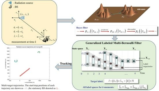
Generalized Labeled Multi-Bernoulli Filter-Based Passive Localization and Tracking of Radiation Sources Carried by Unmanned Aerial Vehicles

Abstract

This paper discusses a key technique for passive localization and tracking of radiation sources, which obtains the motion trajectory of radiation sources carried by unmanned aerial vehicles (UAVs) by continuously or periodically localizing it without the active participation of the radiation sources. However, the existing methods have some limitations in complex signal environments and non-stationary wireless propagation that impact the accuracy of localization and tracking. To address these challenges, this paper extends the $\delta$-generalized labeled multi-Bernoulli (GLMB) filter to the scenario of passive localization and tracking based on the random finite-set (RFS) framework and provides the extended Kalman filter (EKF) and unscented Kalman filter (UKF) implementations of the $\delta$-GLMB filter, which fully take into account the nonlinear motion of the radiation source. By modeling the “obstacle scenario” and the influence of external factors (e.g., weather, terrain), our proposed GLMB filter can accurately track the target and capture its motion trajectory. Simulation results verify the effectiveness of the GLMB filter in target identification and state tracking.

1. Introduction

The goal of passive localization and tracking is to continuously or periodically localize the target or radiation source without the active participation of the target or radiation source, thus obtaining the motion trajectory of the target or radiation source carried by unmanned aerial vehicles (UAVs) [1]. Passive localization and tracking of radiation sources is a critical technology used to determine the position and motion of wireless signal transmitters without active contact, which has a wide range of applications in various fields, such as wireless communications, radio frequency interference (RFI) monitoring, environmental surveillance, and military reconnaissance [2,3,4]. By analyzing the characteristics of received wireless signals, passive localization and tracking provide valuable insights into the spatial distribution of radiation sources, ensuring efficient spectrum management and enhancing situational awareness.

With the rapid proliferation of wireless devices and communication systems, the electromagnetic spectrum is becoming increasingly congested, leading to challenges in efficient spectrum utilization and interference management [5]. In such complex and dynamic electromagnetic environments, it becomes critical to precisely locate and track the radiation sources. Furthermore, passive techniques prove to be essential in situations where the active detection or engagement of the sources is not feasible or desirable. Also, they provide valuable information about the location and behavior of the radiation source, which enables effective monitoring, interference mitigation, and spectrum allocation.

Recently, researchers have proposed different methods for passive localization and tracking of radiation sources. These approaches can be broadly categorized as follows: (1) Time-of-arrival (TOA) techniques [6,7]—These methods estimate the source location based on the time difference between the arrival of the signal at multiple receivers. By calculating the delay time, the position of the transmitter can be deduced. (2) Angle-of-arrival (AOA) method [8]—The AOA method depends on the observation of the direction of arrival (DOA) of the signal at multiple receiving antennas. By triangulating the angle, the location of the transmitter can be determined. (3) Received-signal-strength (RSS, [6]) approaches—RSS-based methods utilize the strength of the received signal to estimate the distance between the source and the receiver. By combining distance measurements from multiple receivers, the location of the transmitter can be inferred. (4) Time-of-flight (TOF) measurements [9,10]—ToF ranging methods are bi-directional ranging techniques, which primarily use the time of flight of a signal traveling back and forth between two asynchronous transceivers (or reflected surfaces) to measure the distance between nodes. In line-of-sight (LOS) environments, ToF-based ranging methods can compensate for the shortcomings of RSSI-based methods.

However, the above methods have some limitations. Firstly, in a complex multipath signal environment or when there are obstacles between the target and the receiver (when the number of targets observed by the receiver is variable), the accuracy of localization and tracking may be compromised. Secondly, the non-ideal signal propagation results in an increased error, which affects the accuracy of localization and tracking. Finally, wireless signal propagation environments are usually non-stationary and impacted by factors such as weather, terrain, and other wireless devices. These variations may lead to a change in parameters such as propagation loss, multipath effect, etc., compromising the localization and tracking results. The random finite-set (RFS) method, as introduced by Mahler in [11], offers a solution to the multi-target tracking problem. Bayesian filtering based on RFS theory is adept at dynamically detecting the number of targets and their states, finding extensive applications in various domains [12,13,14,15,16,17,18].

Because of the multi-target Bayesian filter’s numerical complexity, some alternative approaches have been proposed, including the probability hypothesis density (PHD) [19,20,21], cardinality PHD (CPHD) [22,23], and multi-Bernoulli filter [24,25] methods. Nevertheless, these methods do not function as multi-target trackers since they lack the ability to track target trajectories and, consequently, cannot discern the identity information of the targets. Therefore, Vo et al. proposed the RFS-based generalized labeled multi-Bernoulli (GLMB) [26,27,28] and $\delta$-GLMB [29] filters, where the $\delta$-GLMB [29] filter yields stronger results compared to the GLMB filter and is more applicable to the multi-target tracking problem [30,31,32,33,34,35].

In this paper, we extend the $\delta$-GLMB [29] filter to the passive localization and tracking scenarios. The major contributions of this paper are as follows:

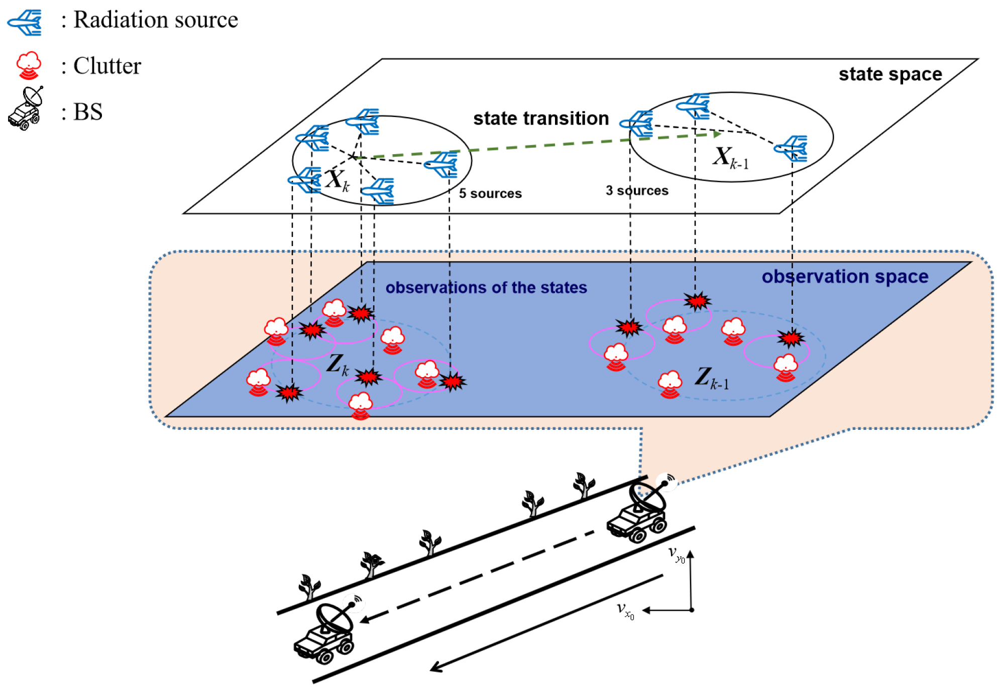
• For the complex electromagnetic environment, we model the “scenario with obstacles between the target and the receiver” as an RFS, in which both the state and the number of targets received by the receiver of the base station change during the observation time.
• The non-stationary wireless signal propagation environment is usually affected by weather, terrain, other wireless devices, etc. Therefore, we model external factors such as weather and terrain (which may impact the information received by the receiver) as a clutter RFS and identify that each clutter generates a false alarm (a false measurement). Our proposed filter is capable of accurately tracking targets of interest from clutter interference and capturing their trajectory onset remarkably well.
• We describe the extended Kalman filter (EKF) and unscented Kalman filter (UKF) implementations of the $\delta$-GLMB filter, which are able to accurately capture the target’s motion state. Moreover, we extend the PHD and CPHD filters to the scenarios of interest in this paper for comparison with the proposed method. Simulation tests verify the effectiveness of the $\delta$-GLMB filter for target number identification and state tracking.

This paper is structured as follows. In Section 2, we provide an overview of the relevant background, encompassing the dynamic physics model of a single target, measurement model, multi-target random finite-set (RFS) system model, Bayesian multi-target recursion, and $\delta$-GLMB filter. Section 3 presents a concise overview of the nonlinear recursive implementation of the $\delta$-GLMB filter for passive localization and tracking. Section 4 and Section 5 offer some numerical examples and conclusions, respectively. Additionally, Appendices Appendix A and Appendix B present some fundamental theories. We use upper-case (lower-case) bold characters to indicate matrices (vectors). Some symbols and their implications are given in Abbreviations.

2. Background

This section presents the background relevant to passive localization and tracking, including the dynamic physical model of the target radiation source, measurement model, multi-target random finite-set system model for time-varying multi-radiation source tracking, fundamental theories of Bayesian multi-target recursion, and $\delta$-GLMB filter. Additionally, some random finite-set fundamentals involved in this section are supplemented in Appendix B.

2.1. Dynamic Physics Model

Assume that the state of the n-th target is ${\mathbf{x}}_k^n={[x_k^n,{\dot{x}}_k^n,y_k^n,{\dot{y}}_k^n]}^T,n=1,2,\dots ,N_k$, where $x_k$ and $y_k$ are the Cartesian coordinates of the x and y positions, respectively; ${\dot{x}}_k^n$ and ${\dot{y}}_k^n$ denote the velocities in the x and y directions; and $N_k$ denotes the total number of radiation sources. The dynamic physics model (also known as the state equation) is given as follows:

$${\mathbf{x}}_k^n={\mathbf{F}}_k{\mathbf{x}}_{k-1}^n+{\mathbf{\omega }}_{k-1},$$

(1)

where ${\mathbf{F}}_k$ is the transfer matrix, and its type determines the kinematic model of the target ${\mathbf{x}}_{k-1}$ at time k. ${\mathbf{\omega }}_{k-1}$ denotes the state noise, which comes from the fact that there is a certain error between our physical model and the actual trajectory of the target, and this part of the error is denoted by ${\mathbf{\omega }}_{k-1}$. Since ${\mathbf{\omega }}_{k-1}$ is a random quantity, we generally describe it by its statistic. In this case, we describe it by the covariance matrix ${\mathbf{Q}}_{k-1}$ of ${\mathbf{\omega }}_{k-1}$. If the value of ${\mathbf{Q}}_{k-1}$ is smaller, we consider that the system model we built is closer to the actual target trajectory, i.e., at this point, we trust the predicted value obtained from the system model more than the measurement.

It is important to note that the value of ${\mathbf{Q}}_{k-1}$ is not as small as possible. There are two reasons for this: (1) the compatibility between the dynamic model and the actual motion trajectory of the target; and (2) whether the target is in nonlinear motion or not. This point is explained later in the simulations. Additionally, the state noise ${\mathbf{\omega }}_{k-1}$ is more accurately expressed as ${\Gamma }_k$ multiplied by ${\mathbf{v}}_{k-1}$. The process noise input matrix ${\Gamma }_k$ is given by

$${\Gamma }_k=\left[\begin{array}{cc}\Delta T^2/\phantom{\Delta T^{2}2}2& 0\\ \Delta T& 0\\ 0& \Delta T^2/\phantom{\Delta T^{2}2}2\\ 0& T\end{array}\right],$$

(2)

where $\Delta T$ is the time-sampling interval. Then, the dynamic physics model (Equation (1)) can be expressed as

$${\mathbf{x}}_k^n={\mathbf{F}}_k{\mathbf{x}}_{k-1}^n+{\Gamma }_k{\mathbf{v}}_{k-1},$$

(3)

where ${\mathbf{v}}_{k-1}={\left[{\delta }_x,{\delta }_y\right]}^T$ is the process noise and ${\mathbf{v}}_{k-1}\sim \mathcal{N}\left(\mathbf{0},{\mathbf{Q}}_{k-1}\right)$.

Remark 1.

In this paper, we introduce a labeled scheme for each source, assigning a unique label l to each source. This label is constructed as an ordered pair $(k,n)$, where n represents the index of targets that originated at time k. We define the labeled space for all targets up to time k as a disjoint union ${\mathbb{L}}_k={\bigcup }_{h=1}^k{\mathbb{B}}_h$, where ${\mathbb{B}}_h$ is the labeled space of targets born at time h (notably, ${\mathbb{L}}_k={\mathbb{L}}_{k-1}\cup {\mathbb{B}}_k$). Then, the states presented in Equation (1) can be denoted as labeled vectors ${\mathbf{x}}_k^n:=\left({\mathbf{x}}_k^n,l_k^n\right)$, where $l_k^n=\left(k,n\right)$.

2.2. Measurement Model

Figure 1 illustrates a two-dimensional passive localization model between a base station (BS) and multi-radiation sources, where both the base station and the radiation source are moving. Using the starting position of the base station $(x_0,y_0)$ as the reference point to build a two-dimensional plane rectangular coordinate system, the measurement information obtained by the BS at time k is

$${\mathbf{z}}_k={\left[{\theta }_k,{\dot{\theta }}_k,{\dot{f}}_k\right]}^T+{\mathbf{n}}_k,$$

(4)

with

$${\theta }_k=arctan\frac{y_k-y_{0k}}{x_k-x_{0k}},$$

(5)

$${\dot{\theta }}_k=\frac{\left({\dot{y}}_k-v_{y_0}\right)\left(x_k-x_{0k}\right)-\left({\dot{x}}_k-v_{x_0}\right)\left(y_k-y_{0k}\right)}{\sqrt{{\left(x_k-x_{0k}\right)}^2+{\left(y_k-y_{0k}\right)}^2}},$$

(6)

$${\dot{f}}_k=-\frac{{\left(\left({\dot{y}}_k-v_{y_0}\right)\left(x_k-x_{0k}\right)-\left({\dot{x}}_k-v_{x_0}\right)\left(y_k-y_{0k}\right)\right)}^2}{\lambda {\left({\left(x_k-x_{0k}\right)}^2+{\left(y_k-y_{0k}\right)}^2\right)}^{3/2}},$$

(7)

where ${\theta }_k$, ${\dot{\theta }}_k$, and ${\dot{f}}_k$ are the azimuth, angular velocity, and Doppler frequency change-rate measurements, respectively. $\lambda$ denotes the carrier wavelength. Appendix A provides the specific calculations of ${\theta }_k$, ${\dot{\theta }}_k$, and ${\dot{f}}_k$. $(x_{0k},y_{0k})$ is the position of the base station at time k with velocity $(v_{x_0},v_{y_0})$; ${\mathbf{n}}_k={\left[{\delta }_{{\theta }_k},{\delta }_{{\dot{\theta }}_k},{\delta }_{{\dot{f}}_k}\right]}^T$ denotes the measurement noise, where ${\delta }_{{\theta }_k}$, ${\delta }_{{\dot{\theta }}_k}$, and ${\delta }_{{\dot{f}}_k}$ are the azimuth error, angular velocity error, and Doppler frequency change-rate error that are independent of each other; and ${\mathbf{n}}_k\sim N\left(\mathbf{0},{\mathbf{R}}_k\right)$, with ${\mathbf{R}}_k=diag\left({\sigma }_{{\theta }_k}^2,{\sigma }_{{\dot{\theta }}_k}^2,{\sigma }_{{\dot{f}}_k}^2\right)$. ${\sigma }_{{\theta }_k}$, ${\sigma }_{{\dot{\theta }}_k}$, and ${\sigma }_{{\dot{f}}_k}$ are the (statistics) standard deviations of ${\delta }_{{\theta }_k}$, ${\delta }_{{\dot{\theta }}_k}$, and ${\delta }_{{\dot{f}}_k}$, respectively.

According to the geometric theory of kinematics, the distance $r_k$ between the base station $(x_{0k},y_{0k})$ and the target radiation source ${\mathbf{x}}_k$ can be expressed as

$$r_k=\frac{-\lambda {\dot{f}}_k}{{\dot{\theta }}_k^2},$$

(8)

with the above equation being the expression for passive ranging. Finally, the estimated position of the target radiation source is derived from the azimuth information

$$\left\{\begin{array}{c}{\tilde{x}}_k=x_{0k}+r_{k}cos{\theta }_k\hfill \\ {\tilde{y}}_k=y_{0k}+r_{k}sin{\theta }_k\hfill \end{array}.\right.$$

(9)

Remark 2.

Obviously, Equation (9) is over-idealized. In practical passive localization scenarios, two key issues need to be addressed: (1) the kinematic state of the target radiation sources and their number may be variable during the observation time; and (2) the interference signals from other uninterested targets (called clutter, as shown in Figure 1) can also be observed by the base station. The strength of the clutter signal affects the final tracking performance. Our task is to track the target location from a cluttered environment. In the next two subsections, we briefly describe the multi-target RFS system model and Bayesian multi-target recursion.

2.3. Multi-Target RFS System Model

Based on RFS theory [19], the multi-target state RFS ${\mathbf{X}}_k$ and observation RFS ${\mathbf{Z}}_k$ can be expressed as

$$\begin{array}{c}{\mathbf{X}}_k=\left\{{\mathbf{x}}_{k,1},\cdots ,{\mathbf{x}}_{k,N_k}\right\}\in \mathcal{F}\left(\mathcal{X}\right),\hfill \\ {\mathbf{Z}}_k=\left\{{\mathbf{z}}_{k,1},\cdots ,{\mathbf{z}}_{k,M_k}\right\}\in \mathcal{F}\left(\mathcal{Z}\right).\hfill \end{array}$$

(10)

where $N_k$ and $M_k$ are the number of targets and the measurements at time k, $\mathcal{X}\in {\mathbb{R}}^{n_x}$ denotes the state space, and $\mathcal{Z}\in {\mathbb{R}}^{n_z}$ is the measurement space.

Using RFS theory, it can be seen that $N_k$ and $M_k$ are time-varying, which enables us to construct the basic model of the problem we are aiming to solve. Given a random set of multi-target state ${\mathbf{X}}_{k-1}$ at time $k-1$, each state ${\mathbf{x}}_{k-1}\in {\mathbf{X}}_{k-1}$ either survives with probability $P_{S,k}\left({\mathbf{x}}_{k-1}\right)$ and travels along the kinematic density $f_{k|k-1}\left({\mathbf{x}}_{k-1}\right)$ to ${\mathbf{x}}_k$, or disappear with death probability $1-P_{S,k}\left({\mathbf{x}}_{k-1}\right)$. Moreover, there are also new targets that appear in the target state space with a newborn probability $P_{B,k}\left({\mathbf{x}}_{B,k}\right)$. Then, the multi-target RFS ${\mathbf{X}}_k$ is in the form of a union set

$${\mathbf{X}}_k=\left\{\bigcup _{{\mathbf{x}}_{k-1}\in {\mathbf{X}}_{k-1}}{\mathbf{S}}_{k|k-1}\left({\mathbf{x}}_{k-1}\right)\right\}\cup {\mathbf{B}}_k,$$

(11)

where ${\mathbf{B}}_k$ represents the multi-Bernoulli RFS of spontaneous newborn targets (provided in Appendix B) and ${\mathbf{S}}_{k|k-1}$ denotes the survival targets. The multi-target RFS integrates the target’s motion, including the appearance of new targets as well as their disappearance. It is assumed that the RFSs described by Equation (11) are independent of each other, i.e., ${\mathbf{X}}_k$ is the proposed multi-Bernoulli RFS based on ${\mathbf{X}}_{k-1}$.

At time k, for a given target ${\mathbf{x}}_k$ from the set ${\mathbf{X}}_k$, it follows one of two scenarios: either it is detected by the BS with a probability of $P_{D,k}\left({\mathbf{x}}_k\right)$ and produces a measurement ${\mathbf{z}}_k$ with likelihood $g_k\left({\mathbf{z}}_k\left|{\mathbf{x}}_k\right.\right)$, or it is undetected with probability $1-P_{D,k}\left({\mathbf{x}}_k\right)$. In other words, each state results in a Bernoulli RFS denoted as ${\Theta }_k\left({\mathbf{x}}_k\right)$, characterized by $r=P_{D,k}\left({\mathbf{x}}_k\right)$ and $p(·)=g_k\left(·\left|{\mathbf{x}}_k\right.\right)$. Additionally, the BS also encounters a collection of clutter represented as a Poisson RFS ${\mathbf{K}}_k$ with an intensity function ${\kappa }_k(·)$. Consequently, the multi-target measurement ${\mathbf{Z}}_k$ is

$${\mathbf{Z}}_k=\left\{\bigcup _{{\mathbf{x}}_k\in {\mathbf{X}}_k}{\Theta }_k\left(x_k\right)\right\}\cup {\mathbf{K}}_k,$$

(12)

where the RFSs comprising the union in (12) are independent of each other.

2.4. $\delta$-GLMB FILTER

The labeled RFS form of the multi-target state in Equation (10) is given in Appendix B.3, and the RFSs for $\delta$-GLMB are also given in Appendix B.4. For simplicity, let ${\mathbb{L}}_{+}\stackrel{\Delta }{=}\mathbb{L}\cup \mathbb{B}$, $\mathbb{L}\stackrel{\Delta }{=}{\mathbb{L}}_{0:k}$, $\mathbb{B}\stackrel{\Delta }{=}{\mathbb{L}}_{k+1}$, $\mathit{\pi }\stackrel{\Delta }{=}{\mathit{\pi }}_k$, ${\mathit{\pi }}_{+}\stackrel{\Delta }{=}{\mathit{\pi }}_{k+1|k}$, $g\stackrel{\Delta }{=}{g}_k$, $f\stackrel{\Delta }{=}{f}_{k+1|k}$, $\mathbf{X}\stackrel{\Delta }{=}{\mathbf{X}}_k$, $\mathbf{Z}\stackrel{\Delta }{=}{\mathbf{Z}}_k$.

The numerical implementation of the GLMB RFS becomes notably more challenging under Bayesian recursion. However, drawing insights from [26,29], the $\delta$-GLMB RFS (refer to Appendix B.4) emerges as a specialized variant of the GLMB RFS, offering a simplified numerical approach that is exceptionally well suited for multi-target tracking applications. Then, the $\delta$-GLMB prediction density at time $k+1$ is

$$\begin{array}{c}{\mathit{\pi }}_{+}\left({\mathbf{X}}_{+}\right)=\Delta \left({\mathbf{X}}_{+}\right)\times {\displaystyle \sum _{\left(I_{+},\vartheta \right)\in \mathcal{F}\left({\mathbb{L}}_{+}\right)\times \Xi }}{{\omega }_{+}}^{\left(I_{+},\vartheta \right)}{\delta }_{I_{+}}\left[\mathcal{L}\left({\mathbf{X}}_{+}\right)\right]{{\displaystyle \left[{p_{+}}^{\left(\vartheta \right)}\right]}}^{{\mathbf{X}}_{+}},\hfill \end{array}$$

(13)

where

$${{\omega }_{+}}^{\left(I_{+},\vartheta \right)}={\omega }_S^{\vartheta }\left(I_{+}\cap \mathbb{L}\right){\omega }_B\left(I_{+}\cap \mathbb{B}\right),$$

(14)

$${\omega }_S^{\vartheta }\left(L\right)={\left[{\eta }_S^{\left(\vartheta \right)}\right]}^L\sum _{L\subseteq I}{1}_I\left(L\right){\left[1-{\eta }_S^{\left(\vartheta \right)}\right]}^{I-L}{\omega }^{\left(I,\vartheta \right)},$$

(15)

$${\eta }_S^{\left(\vartheta \right)}\left(l\right)=\int 〈P_S\left(·,l\right)f\left(\mathbf{x}|·,l\right),p^{\left(\vartheta \right)}\left(·,l\right)〉d\mathbf{x},$$

(16)

$$p_{+}^{\left(\vartheta \right)}\left(\mathbf{x},l\right)=1_{\mathbb{L}}\left(l\right)p_{+,S}^{\left(\vartheta \right)}\left(\mathbf{x},l\right)+1_{\mathbb{B}}\left(l\right)p_B\left(\mathbf{x},l\right),$$

(17)

$$p_{+,S}^{\left(\vartheta \right)}\left(\mathbf{x},l\right)=\frac{〈P_S\left(·,l\right)f\left(\mathbf{x}|·,l\right),p^{\left(\vartheta \right)}\left(·,l\right)〉}{{\eta }_S^{\left(\vartheta \right)}\left(l\right)}.$$

(18)

In the above equations, the following notations are used:

• $I_{+}$ is a collection of predicted trajectory labels within the set $\mathcal{F}\left({\mathbb{L}}_{+}\right)$. Each tuple $\left(I_{+},\vartheta \right)\in \mathcal{F}\left({\mathbb{L}}_{+}\right)\times \Xi$ is a prediction hypothesis with probability ${{\omega }_{+}}^{\left(I_{+},\vartheta \right)}$. $\vartheta \stackrel{\Delta }{=}\left({\theta }_1,\cdots ,{\theta }_k\right)\in \Xi \stackrel{\Delta }{=}{\Theta }_1\times {\Theta }_2\times \cdots \times {\Theta }_k$ represents the historical association mapping.
• ${\omega }_B\left(I_{+}\cap \mathbb{B}\right)$ represents the weight associated with the newborn trajectory labels, where $I_{+}\cap \mathbb{B}\ne \varnothing$ and $\mathbb{B}$ denote the labeled space for newborn sources. $p_B\left(\mathbf{x},l\right)$ is the probability density function (PDF) for the newborn source $\mathbf{x}$ with label l. ${\omega }_S^{\vartheta }\left(L\right)$ is the weight of the survival label set.
• $p_{+}^{\left(\vartheta \right)}\left(\mathbf{x},l\right)$ is the prediction PDF, and $p^{\vartheta }\left(·,l\right)$ is the update PDF. $f\left(\mathbf{x}|·,l\right)$ denotes the transition kinematic density, and $P_S\left(·,l\right)$ represents the survival probability.

At time $k+1$, the multi-target prediction density adheres to the $\delta$-GLMB formulation, as defined in Equation (13). Then, the multi-target filtering (update) density is also a $\delta$-GLMB structure, i.e.,

$$\begin{array}{c}\pi \left(\mathbf{X}|\mathbf{Z}\right)\propto \Delta \left(\mathbf{X}\right){\displaystyle \sum _{\left(I,\vartheta \right)\in \mathcal{F}\left(\mathbb{L}\right)\times \Xi }}{\displaystyle \sum _{\theta \in \Theta \left(I\right)}}{\omega }^{\left(I,\vartheta ,\theta \right)}\left(\mathbf{Z}\right)\times {\delta }_I\left(\mathcal{L}\left(\mathbf{X}\right)\right){\left[p^{\left(\vartheta ,\theta \right)}\left(·|\mathbf{Z}\right)\right]}^{\mathbf{X}},\hfill \end{array}$$

(19)

where

$${\omega }^{\left(I,\vartheta ,\theta \right)}\left(\mathbf{Z}\right)\propto {\left[{\mu }_{\mathbf{Z}}^{\left(\vartheta ,\theta \right)}\right]}^I{\omega }^{\left(I,\vartheta \right)},$$

(20)

$${\mu }_{\mathbf{Z}}^{\left(\vartheta ,\theta \right)}\left(l\right)=〈p_{+}^{\left(\vartheta \right)}(·,l),{\psi }_{\mathbf{Z}}\left(·,l;\theta \right)〉,$$

(21)

$${\psi }_{\mathbf{Z}}\left(\mathbf{x},l;\theta \right)=\left\{\begin{array}{l}\begin{array}{c}\frac{P_D\left(\mathbf{x},l\right)g\left({\mathbf{z}}_{\theta \left(l\right)}|\mathbf{x},l\right)}{\kappa \left({\mathbf{z}}_{\theta \left(l\right)}\right)}, \theta \left(l\right)>0\end{array}\\ 1-P_D\left(\mathbf{x},l\right), \theta \left(l\right)=0\end{array}\right..$$

(22)

$$p^{\left(\vartheta ,\theta \right)}\left(\mathbf{x},l|\mathbf{Z}\right)=\frac{p_{+}^{\left(\vartheta \right)}\left(\mathbf{x},l\right){\psi }_{\mathbf{Z}}\left(\mathbf{x},l;\theta \right)}{{\mu }_{\mathbf{Z}}^{\left(\vartheta ,\theta \right)}\left(l\right)},$$

(23)

where $\Theta$ represents the measurement association mapping, denoted as $\theta :\mathbb{L}\to \left\{0,1,\cdots ,\left|\mathbf{Z}\right|\right\}$, and $\theta$ adheres to the condition that $\theta \left(i\right)=\theta \left(j\right)>0\Rightarrow i=j$. $\Theta \left(I\right)$ is the subset of the association mapping associated with I. $\left(I,\vartheta ,\theta \right)$ denotes the hypothesis when I possesses an association mapping history $\vartheta \stackrel{\Delta }{=}\left({\theta }_1,\cdots ,{\theta }_{k+1}\right)\in \Xi \stackrel{\Delta }{=}{\Theta }_1\times {\Theta }_2\times \cdots \times {\Theta }_{k+1}$, with ${\omega }^{\left(I,\vartheta ,\theta \right)}$ indicating the corresponding weight assigned to this hypothesis. $P_D\left(\mathbf{x},l\right)$ denotes the detection probability, and $g\left({\mathbf{z}}_{\theta \left(l\right)}|\mathbf{x},l\right)$ is the likelihood function of state $\mathbf{x}$.

3. Nonlinear $\mathbf{\delta }$-GLMB Filter for Passive Localization and Tracking

We explore the expansion of the $\delta$-GLMB filter to accommodate nonlinear target models. Specifically, we need to relax the state and observation process Equations (1) and (4) to incorporate the nonlinear model Equations (24) and (25), given by

$${\mathbf{x}}_k=f_k\left({\mathbf{x}}_{k-1},{\mathbf{v}}_{k-1}\right),$$

(24)

$${\mathbf{z}}_k=h_k\left({\mathbf{x}}_k,{\mathbf{n}}_k\right),$$

(25)

where $f_k$ and $h_k$ are the nonlinear functions and ${\mathbf{v}}_k$ and ${\mathbf{n}}_k$ denote the process and measurement noise, both with zero mean covariance ${\mathbf{Q}}_{k-1}$ and ${\mathbf{R}}_k$, respectively. The posterior density cannot be described in Gaussian form because of the nonlinearity presented by $f_k$ and $h_k$. Nevertheless, we can adjust the $\delta$-GLMB filter ([29]) to fit this nonlinear Gaussian model. For the nonlinear Gaussian model, we propose two nonlinear implementations (EKF and UKF) for the $\delta$-GLMB filter.

3.1. $\delta$-GLMB Prediction for Nonlinear Gaussian Model

The predicted density presented in Equation (13) is a compact form, but in Equation (20), it requires the summation of all supersets of L, and consequently, is more difficult to compute. To this end, [26] provided an equivalent version as follows:

$$\begin{array}{c}{\pi }_{+}\left({\mathbf{X}}_{+}\right)=\Delta \left({\mathbf{X}}_{+}\right){\displaystyle \sum _{\left(I,\vartheta \right)\in \mathcal{F}\left(\mathbb{L}\right)\times \Xi }}{\displaystyle \sum _{J\in \mathcal{F}\left(I\right)}}{\omega }_S^{\left(I,\vartheta \right)}\left(J\right){\displaystyle \sum _{L\in \mathcal{F}\left(\mathbb{B}\right)}}{\omega }_B\left(L\right){\delta }_{J\cup L}\left(\mathcal{L}\left({\mathbf{X}}_{+}\right)\right){\left[{p_{+}}^{\left(\vartheta \right)}\right]}^{{\mathbf{X}}_{+}},\hfill \end{array}$$

(26)

where $J\subseteq I,L\subseteq \mathbb{B}$. For the newborn radiation sources, the labeled multi-Bernoulli newborn model is used

$${\omega }_B\left(L\right)=\prod _{l\in \mathbb{B}}\left(1-r_B^{\left(l\right)}\right)\prod _{l\in L}\frac{1_{\mathbb{B}}\left(l\right)r_B^{\left(l\right)}}{\left(1-r_B^{\left(l\right)}\right)},$$

(27)

$$p_B\left(\mathbf{x},l\right):=p_B^{\left(l\right)}\left(\mathbf{x}\right),$$

(28)

where $r_B^{\left(l\right)}$ denotes the existence probability with newborn label l with PDF $p_B^{\left(l\right)}\left(\mathbf{x}\right)$. The weight ${\omega }_S^{(I,\vartheta )}\left(J\right)$ is the survival probability of the labels in J. Since the new label space $\mathbb{B}$ cannot contain any labels of the surviving target, then $I\cap \mathbb{B}=\varnothing$.

3.1.1. K-Shortest Path Algorithm

Given the hypothesis $(I,\vartheta )$, the surviving label set weight ${\omega }_S^{(I,\vartheta )}\left(J\right)$ is

$${\omega }_S^{(I,\vartheta )}\left(J\right)={\omega }^{\left(I,\vartheta \right)}{\left[1-{\mathit{\eta }}_S^{\left(\vartheta \right)}\right]}^I{\left[\frac{{\mathit{\eta }}_S^{\left(\vartheta \right)}}{1-{\mathit{\eta }}_S^{\left(\vartheta \right)}}\right]}^J.$$

(29)

Figure 2 shows the directed graph of the K-shortest path algorithm, and the detailed process can be found in [29]. By stretching the directed graph in Figure 2 to include survival and newborn nodes with appropriate costs, we can determine the total K-best components. However, the value of newborn weights ${\omega }_B\left(L\right)$ is often much smaller than the survival weights ${\omega }_S^{(I,\vartheta )}\left(L\right)$, leading to the discarding of many newborn components and making it challenging to detect newborn targets. In contrast, a much larger value of K is desirable to preserve the newborn hypothesis and prevent the rejection of new trajectories. Nevertheless, to mitigate computational complexity, the separated pruning strategy ensures that there exists a certain number of newborn hypothesis components exist to process the new trajectories with a high degree of parallelism.

3.1.2. Computing the Predicted Parameter Sets (EKF Implementation)

For the EKF approximation, the PDF $p^{\left(\vartheta \right)}(·,l)$ can be expressed as the Gaussian distribution parameter sets ${\left\{{\omega }_i^{\left(\vartheta \right)}\left(l\right),\mathcal{N}\left(\mathbf{x};{\mathbf{m}}_i^{\left(\vartheta \right)}\left(l\right),{\mathbf{P}}_i^{\left(\vartheta \right)}\left(l\right)\right)\right\}}_{i=1}^{J^{\left(\vartheta \right)}\left(l\right)}$, with mean ${\mathbf{m}}_i^{\left(\vartheta \right)}$ and covariance ${\mathbf{P}}_i^{\left(\vartheta \right)}\left(l\right)$, Then, we have

$${\eta }_S^{\left(\vartheta \right)}\left(l\right)=P_S\left(·,l\right),$$

(30)

$$\begin{array}{c}{p}_{+}^{\left(\vartheta \right)}(\mathbf{x},l)=1_{\mathbb{L}}\left(l\right){\displaystyle \sum _{i=1}^{J^{\left(\vartheta \right)}\left(l\right)}}{\omega }_i^{\left(\vartheta \right)}\left(l\right)\mathcal{N}\left(\mathbf{x};{\mathbf{m}}_{S,i}^{\left(\vartheta \right)}\left(l\right),{\mathbf{P}}_{S,i}^{\left(\vartheta \right)}\left(l\right)\right)+1_{\mathbb{B}}\left(l\right)p_B^{\left(l\right)}\left(\mathbf{x}\right),\hfill \end{array}$$

(31)

with

$${\mathbf{m}}_{S,i}^{\left(\vartheta \right)}\left(l\right)=f\left({\mathbf{m}}_i^{\left(\vartheta \right)}\left(l\right),\mathbf{0}\right),$$

(32)

$${\mathbf{P}}_{S,i}^{\left(\vartheta \right)}\left(l\right)={\tilde{\mathbf{F}}\left(l\right)\mathbf{P}}_i^{\left(\vartheta \right)}\left(l\right){\tilde{\mathbf{F}}\left(l\right)}^T+\Gamma \mathbf{Q}{\Gamma }^T,$$

(33)

$$\tilde{\mathbf{F}}\left(l\right)=\frac{\partial f\left(\mathbf{x},\mathbf{0}\right)}{\partial \mathbf{x}}\left|{ }_{\mathbf{x}={\mathbf{m}}_i^{\left(\vartheta \right)}\left(l\right)}\right..$$

(34)

3.1.3. Computing the Predicted Parameter Sets (UKF Implementation)

The UKF approximation proposes a recursive nonlinear approach to the $\delta$-GLMB filter, utilizing the unscented transform (UT). For the i-th Gaussian component $\mathcal{N}\left(\mathbf{x};{\mathbf{m}}_i^{\left(\vartheta \right)}\left(l\right),{\mathbf{P}}_i^{\left(\vartheta \right)}\left(l\right)\right)$, the UT is employed with mean ${\mathit{\mu }}_i^{\left(\vartheta \right)}\left(l\right)$ and covariance ${\mathbf{M}}_i^{\left(\vartheta \right)}\left(l\right)$ to provides the sigma points set ${\left\{{\mathbf{y}}_{i,g}^{\left(\vartheta \right)}\left(l\right),u_g\right\}}_{g=0}^G$, where

$${\mathit{\mu }}_i^{\left(\vartheta \right)}\left(l\right)=\left[{\mathbf{m}}_i^{\left(\vartheta \right)}\left(l\right);{\mathbf{0}}_{2\times 1}\right],$$

(35)

$${\mathbf{M}}_i^{\left(\vartheta \right)}\left(l\right)=diag\left({\mathbf{P}}_i^{\left(\vartheta \right)}\left(l\right),\mathbf{Q}\right),$$

(36)

and $u_g$ is the weight of g-th sigma point ${\mathbf{y}}_{i,g}^{\left(\vartheta \right)}\left(l\right)$. Then, these sigma points are divided into

$${\mathbf{y}}_{i,g}^{\left(\vartheta \right)}\left(l\right)=\left[{\mathbf{x}}_{i,g}^{\left(\vartheta \right)}\left(l\right);{\mathbf{v}}_{i,g}^{ }\left(l\right)\right]$$

(37)

for $g=1,\cdots ,G$, and the operations are performed as follows:

• Predict the sigma points: ${\tilde{\mathbf{x}}}_{i,g}^{\left(\vartheta \right)}\left(l\right)=f\left({\mathbf{x}}_{i,g}^{\left(\vartheta \right)}\left(l\right),{\mathbf{v}}_{i,g}^{ }\left(l\right)\right)$.
• Use the given approximation Equations (38) and (39) instead of Equations (32) and (33) in the EKF implementation:

  $${\mathbf{m}}_{S,i}^{\left(\vartheta \right)}\left(l\right)=\sum _{g=1}^G{u}_g{\tilde{\mathbf{x}}}_{i,g}^{\left(\vartheta \right)}\left(l\right),$$

  (38)

  $$\begin{array}{c}{\mathbf{P}}_{S,i}^{\left(\vartheta \right)}\left(l\right)={\displaystyle \sum _{g=1}^G}{u}_g\left({\tilde{\mathbf{x}}}_{i,g}^{\left(\vartheta \right)}\left(l\right)-{\mathbf{m}}_{S,i}^{\left(\vartheta \right)}\left(l\right)\right){\left({\tilde{\mathbf{x}}}_{i,g}^{\left(\vartheta \right)}\left(l\right)-{\mathbf{m}}_{S,i}^{\left(\vartheta \right)}\left(l\right)\right)}^T.\hfill \end{array}$$

  (39)

3.1.4. Pruning the Predicted Density

Given the $\delta$-GLMB filter density with parameter sets ${\left\{\left(I^{\left(h\right)},{\vartheta }^{\left(h\right)},{\omega }^{\left(h\right)},p^{\left(h\right)}\right)\right\}}_{h=1}^H$, where $H\in \mathbb{N}$ is the number of all hypotheses, $p^{\left(h\right)}\stackrel{\Delta }{=}{p}^{\left({\vartheta }^{\left(h\right)}\right)}$ and ${\omega }^{\left(h\right)}\stackrel{\Delta }{=}{\omega }^{\left(I^{\left(h\right)},{\vartheta }^{\left(h\right)}\right)}$. The predicted $\delta$-GLMB filter density (13) can be simplified to

$${\mathit{\pi }}_{+}\left({\mathbf{X}}_{+}\right)={\sum }_{h=1}^H{\mathit{\pi }}_{+}^{\left(h\right)}\left({\mathbf{X}}_{+}\right),$$

(40)

$$\begin{array}{c}{\mathit{\pi }}_{+}^{\left(h\right)}\left({\mathbf{X}}_{+}\right)=\Delta \left({\mathbf{X}}_{+}\right){\displaystyle \sum _{J\in I^{\left(h\right)}}}{\displaystyle \sum _{L\in \mathbb{B}}}{\omega }_S^{\left(I^{\left(h\right)},{\vartheta }^{\left(h\right)}\right)}\left(J\right)\times {\omega }_B\left(L\right){\delta }_{J\cup L}\left(\mathcal{L}\left({\mathbf{X}}_{+}\right)\right){\left[{p_{+}}^{\left({\vartheta }^{\left(h\right)}\right)}\right]}^{{\mathbf{X}}_{+}}.\hfill \end{array}$$

(41)

According to [36], the pruning version of the h-th filter density ${\mathit{\pi }}_{+}^{\left(h\right)}$ is

$$\begin{array}{c}{\tilde{\mathit{\pi }}}_{+}^{\left(h\right)}\left({\mathbf{X}}_{+}\right)=\Delta \left({\mathbf{X}}_{+}\right){\displaystyle \sum _{j=1}^{K_S^{\left(h\right)}}}{\displaystyle \sum _{b=1}^{K_B}}{\omega }_{+}^{\left(h,j,b\right)}{\delta }_{J^{\left(h,j\right)}\cup L^{\left(b\right)}}\left(\mathcal{L}\left({\mathbf{X}}_{+}\right)\right){\left[p_{+}^{\left(h\right)}\right]}^{{\mathbf{X}}_{+}},\hfill \end{array}$$

(42)

where

$${\omega }_{+}^{\left(h,j,b\right)}\stackrel{\Delta }{=}{\omega }_S^{\left(I^{\left(h\right)},{\vartheta }^{\left(h\right)}\right)}\left(J^{\left(h,j\right)}\right){\omega }_B\left(L^{\left(b\right)}\right),$$

(43)

$$p_{+}^{\left(h\right)}\stackrel{\Delta }{=}{p}_{+}^{\left({\vartheta }^{\left(h\right)}\right)}.$$

(44)

Remark 3.

The specific values for the required number of components $K_S^{\left(h\right)}$ and $K_B$ are generally determined by choosing $K_S^{\left(h\right)}=⌈{\omega }^{\left(h\right)}{J}_{max}⌉$, where $J_{max}$ is the total number of expected hypotheses. Additionally, for $K_B$, the appropriate $K_B$ is chosen so that the pruning result can capture the desired proportion of the required newborn PDF. The details of the pruning process can be found in [29].

3.2. $\delta$-GLMB Update for Nonlinear Gaussian Model

This section outlines the implementation steps of the $\delta$-GLMB update, involving the pruning of the multi-target filter density using the ranked assignment algorithm ([29]) without the need for a thorough computation of all hypotheses and their weights.

3.2.1. Ranked Assignment Algorithm

Enumerating $I=\left\{l_1,\cdots ,l_{\left|I\right|}\right\}$, $Z=\left\{{\mathbf{z}}_1,\cdots ,{\mathbf{z}}_{\left|Z\right|}\right\}$, each association mapping $\theta \in \Theta \left(I\right)$ can be characterized by an assignment matrix $\mathbf{A}$ of dimension $\left|I\right|\times \left|Z\right|$. This matrix consists of 0s and 1s and adheres to the rule that each row (or column) sums to either 0 or 1. $A_{ij}=1$ denotes that the j-th measurement is assigned to track $l_i$, i.e., $\theta \left(l_i\right)=j$.

The cost matrix ${\mathbf{C}}_Z^{\left(I,\vartheta \right)}$ is constructed as follows:

$${\mathbf{C}}_Z^{\left(I,\vartheta \right)}=\left[\begin{array}{ccc}{c}_{1,1}& \cdots & c_{1,\left|Z\right|}\\ ⋮& & ⋮\\ c_{\left|I\right|,1}& \cdots & c_{\left|I\right|,\left|Z\right|}\end{array}\right],$$

(45)

with

$$c_{i,j}=-ln\left[\frac{〈p_{+}^{\left(\vartheta \right)}\left(·,l_i\right),p_D\left(·,l_i\right)g\left({\mathbf{z}}_j|·,l_i\right)〉}{〈p_{+}^{\left(\vartheta \right)}\left(·,l_i\right),1-p_D\left(·,l_i\right)〉\kappa \left({\mathbf{z}}_j\right)}\right]$$

(46)

being the cost of assigning the j-th measurement to track $l_i$. The assignment matrix $\mathbf{A}$ represents the cost of assigning each measurement to the radiation source and can be expressed as

$$tr\left({\mathbf{A}}^T{\mathbf{C}}_Z^{\left(I,\vartheta \right)}\right)=\sum _{i=1}^{\left|I\right|}\sum _{j=1}^{\left|Z\right|}{C}_{ij}{A}_{ij}.$$

(47)

By substituting Equation (22) into (21), we obtain the cost associated with $\mathbf{A}$ (and the corresponding correlation mapping $\theta$) in terms of the filtering hypotheses weights ${\omega }^{\left(I,\vartheta ,\theta \right)}\left(\mathbf{Z}\right)\propto {\left[{\mu }_{\mathbf{Z}}^{\left(\vartheta ,\theta \right)}\right]}^I{\omega }^{\left(I,\vartheta \right)}$, where

$$\begin{array}{c}{\left[{\mu }_{\mathbf{Z}}^{\left(\vartheta ,\theta \right)}\right]}^I=exp\left(-tr\left({\mathbf{A}}^T{\mathbf{C}}_Z^{\left(I,\vartheta \right)}\right)\right){\displaystyle \prod _{l\in I}}〈p^{\left(\vartheta \right)}\left(·,l\right),1-p_D\left(·,l\right)〉.\hfill \end{array}$$

(48)

In essence, the ranked assignment algorithm seeks to minimize the cost of the assignment matrix, enumerated in non-descending order [37,38]. Thus, the optimal assignment problem can be addressed in terms of the cost matrix ${\mathbf{C}}_Z^{\left(I,\vartheta \right)}$, which yields an enumeration ordered in non-increasing ${\left[{\mu }_{\mathbf{Z}}^{\left(\vartheta ,\theta \right)}\right]}^I$.

3.2.2. Calculating the Updated Parameter Sets (EKF Implementation)

The $(i,j)$-th element of ${\mathbf{C}}_Z^{(I,\vartheta )}$ is

$$c_{ij}=-ln\left[\frac{p_D\left(·,l_i\right){\sum }_{n=1}^{J^{\left(\vartheta \right)}\left(l_i\right)}{\omega }_n^{\left(\vartheta \right)}\left(l_i\right)q_n^{\left(\vartheta \right)}\left({\mathbf{z}}_j,l_i\right)}{\left(1-p_D\left(·,l_i\right)\right)\kappa \left({\mathbf{z}}_j\right)}\right].$$

(49)

Moreover, for $(\vartheta ,\theta )$, we have

$${\mu }_{\mathbf{Z}}^{\left(\vartheta ,\theta \right)}\left(l\right)={\sum }_{n=1}^{J^{\left(\vartheta \right)}\left(l\right)}{\omega }_{\mathbf{Z},n}^{\left(\vartheta ,\theta \right)}\left(l\right),$$

(50)

$$\begin{array}{c}{p}^{(\vartheta ,\theta )}(\mathbf{x},l|\mathbf{Z})={\sum }_{n=1}^{J^{\left(\vartheta \right)}\left(l\right)}\frac{{\omega }_{\mathbf{Z},n}^{\left(\vartheta ,\theta \right)}\left(l\right)}{{\mu }_{\mathbf{Z}}^{\left(\vartheta ,\theta \right)}\left(l\right)}\mathcal{N}\left(\mathbf{x};{\mathbf{m}}_{\mathbf{Z},n}^{\left(\vartheta ,\theta \right)}\left(l\right),{\mathbf{P}}_n^{\left(\vartheta ,\theta \right)}\left(l\right)\right)\hfill \end{array},$$

(51)

with

$${\omega }_{\mathbf{Z},n}^{\left(\vartheta ,\theta \right)}\left(l\right)={\omega }_n^{\left(\vartheta \right)}\left(l\right)\left\{\begin{array}{l}\frac{p_D\left(·,l\right)q_n^{\left(\vartheta \right)}\left({\mathbf{z}}_{\theta \left(l\right)},l\right)}{\kappa \left({\mathbf{z}}_{\theta \left(l\right)}\right)}, \theta \left(l\right)>0\\ 1-p_D\left(·,l\right), \theta \left(l\right)=0\end{array}\right.,$$

(52)

$$q_n^{\left(\vartheta \right)}\left(\mathbf{z},l\right)=\mathcal{N}\left(x;{\tilde{\mathbf{m}}}_n^{\left(\vartheta \right)}\left(l\right),{\tilde{\mathbf{P}}}_n^{\left(\vartheta \right)}\left(l\right)\right),$$

(53)

$${\tilde{\mathbf{m}}}_n^{\left(\vartheta \right)}\left(l\right)={\tilde{\mathbf{H}}\left(l\right)\mathbf{m}}_n^{\left(\vartheta \right)}\left(l\right),$$

(54)

$${\tilde{\mathbf{P}}}_n^{\left(\vartheta \right)}\left(l\right)={\tilde{\mathbf{H}}\left(l\right)\mathbf{P}}_n^{\left(\vartheta \right)}\left(l\right){\tilde{\mathbf{H}}\left(l\right)}^T+\tilde{\mathbf{U}}\left(l\right)\mathbf{R}{\tilde{\mathbf{U}}\left(l\right)}^T,$$

(55)

$$\tilde{\mathbf{H}}\left(l\right)=\frac{\partial h\left(\mathbf{x},\mathbf{0}\right)}{\partial \mathbf{x}}\left|{ }_{\mathbf{x}={\mathbf{m}}_n^{\left(\vartheta \right)}\left(l\right)}\right.,$$

(56)

$$\tilde{\mathbf{U}}\left(l\right)=\frac{\partial h\left({\mathbf{m}}_n^{\left(\vartheta \right)}\left(l\right),\mathbf{n}\right)}{\partial \mathbf{n}}\left|{ }_{\mathbf{n}=\mathbf{0}}\right.,$$

(57)

$$\begin{array}{c}{\mathbf{m}}_{\mathbf{Z},n}^{\left(\vartheta ,\theta \right)}\left(l\right)=\left\{\begin{array}{l}{\mathbf{m}}_n^{\left(\vartheta \right)}\left(l\right)+{\mathbf{K}}_n^{\left(\vartheta ,\theta \right)}\left(l\right)\left({\mathbf{z}}_{\theta \left(l\right)}-{\tilde{\mathbf{m}}}_n^{\left(\vartheta \right)}\left(l\right)\right), \theta \left(l\right)>0\\ {\mathbf{m}}_n^{\left(\vartheta \right)}\left(l\right), \theta \left(l\right)=0\end{array}\right.\end{array},$$

(58)

$${\mathbf{P}}_n^{\left(\vartheta ,\theta \right)}\left(l\right)=\left(\mathbf{I}-{\mathbf{K}}_n^{\left(\vartheta ,\theta \right)}\left(l\right)\tilde{\mathbf{H}}\right){\mathbf{P}}_n^{\left(\vartheta \right)}\left(l\right),$$

(59)

$${\mathbf{K}}_n^{\left(\vartheta ,\theta \right)}\left(l\right)=\left\{\begin{array}{l}{\mathbf{P}}_n^{\left(\vartheta \right)}\left(l\right){\tilde{\mathbf{H}}}^T{\left({\tilde{\mathbf{P}}}_n^{\left(\vartheta \right)}\left(l\right)\right)}^{-1}, \theta \left(l\right)>0\\ \mathbf{0}, \theta \left(l\right)=0\end{array}\right..$$

(60)

3.2.3. Calculating the Updated Parameter Sets (UKF Implementation)

Firstly, for the j-th predicted Gaussian component $\mathcal{N}\left(\mathbf{x};{\mathbf{m}}_{S,j}^{\left(\vartheta \right)}\left(l\right),{\mathbf{P}}_{S,j}^{\left(\vartheta \right)}\left(l\right)\right),j=1,\cdots ,J^{\left(\vartheta \right)}\left(l\right)$, the UT with mean ${\mathit{\mu }}_{Z,j}^{\left(\vartheta \right)}\left(l\right)$ and covariance ${\mathbf{M}}_{Z,j}^{\left(\vartheta \right)}\left(l\right)$ is used to provide the sigma point set ${\left\{{\mathbf{y}}_{Z,J,g}^{\left(\vartheta \right)}\left(l\right)\right\}}_{g=0}^G$ with weight $u_{Z,g}$, where

$${\mathit{\mu }}_{Z,j}^{\left(\vartheta \right)}\left(l\right)=\left[{\mathbf{m}}_{S,j}^{\left(\vartheta \right)}\left(l\right);{\mathbf{0}}_{3\times 1}\right],$$

(61)

$${\mathbf{M}}_i^{\left(\vartheta \right)}\left(l\right)=diag\left({\mathbf{P}}_i^{\left(\vartheta \right)}\left(l\right),\mathbf{R}\right).$$

(62)

Then, the sigma points are divided into

$${\mathbf{y}}_{Z,j,g}^{\left(\vartheta \right)}\left(l\right)=\left[{\mathbf{x}}_{Z,j,g}^{\left(\vartheta \right)}\left(l\right);{\mathbf{n}}_{Z,j,g}^{ }\left(l\right)\right]$$

(63)

for $g=1,\cdots ,G$, and the operations are performed as outlined below.

For the UKF implementation of the updated $\delta$-GLMB density, the predicted measurement sigma points are ${\mathbf{z}}_{j,g}^{\left(\vartheta \right)}\left(l\right)=h\left({\mathbf{x}}_{Z,j,g}^{\left(\vartheta \right)}\left(l\right),{\mathbf{n}}_{Z,j,g}^{ }\left(l\right)\right),j=1,\cdots ,J^{\left(\vartheta \right)}\left(l\right)$. Then, using Equations (64) and (65) instead of Equations (58) and (59) in the EKF update step, and Equations (66) and (67) instead of the original Equations (54) and (55), the update step can be performed for the nonlinear measurement model

$${\mathbf{m}}_{\mathbf{Z},j}^{\left(\vartheta ,\theta \right)}\left(l\right)=\left\{\begin{array}{l}{\mathbf{m}}_{S,j}^{\left(\vartheta \right)}\left(l\right)+{\mathbf{K}}_j^{\left(\vartheta ,\theta \right)}\left(l\right)\left({\mathbf{z}}_{\theta \left(l\right)}-{\tilde{\mathbf{z}}}_{j,g}^{\left(\vartheta \right)}\left(l\right)\right), \theta \left(l\right)>0\\ {\mathbf{m}}_{S,j}^{\left(\vartheta \right)}\left(l\right), \theta \left(l\right)=0\end{array}\right.,$$

(64)

$${\tilde{\mathbf{P}}}_j^{\left(\vartheta ,\theta \right)}\left(l\right)={\mathbf{P}}_{S,j}^{\left(\vartheta \right)}\left(l\right)-{\mathbf{G}}_{xz}\left(l\right){\left({\mathbf{S}}_{zz}\left(l\right)\right)}^{-1}{\mathbf{G}}_{xz}\left(l\right),$$

(65)

with

$${\tilde{\mathbf{z}}}_{j,g}^{\left(\vartheta \right)}\left(l\right)=\sum _{g=0}^G{u}_{Z,g}{\mathbf{z}}_{j,g}^{\left(\vartheta \right)}\left(l\right),$$

(66)

$$\begin{array}{c}{\mathbf{S}}_{zz}\left(l\right)={\displaystyle \sum _{g=0}^G}{u}_g\left({\mathbf{z}}_{j,g}^{\left(\vartheta \right)}\left(l\right)-{\tilde{\mathbf{z}}}_{j,g}^{\left(\vartheta \right)}\left(l\right)\right){\left({\mathbf{z}}_{j,g}^{\left(\vartheta \right)}\left(l\right)-{\tilde{\mathbf{z}}}_{j,g}^{\left(\vartheta \right)}\left(l\right)\right)}^T,\hfill \end{array}$$

(67)

$$\begin{array}{c}{\mathbf{G}}_{xz}\left(l\right)={\displaystyle \sum _{g=0}^G}{u}_{Z,g}\left({\mathbf{x}}_{Z,j,g}^{\left(\vartheta \right)}\left(l\right)-{\mathbf{m}}_{S,i}^{\left(\vartheta \right)}\left(l\right)\right){\left({\mathbf{z}}_{j,g}^{\left(\vartheta \right)}\left(l\right)-{\tilde{\mathbf{z}}}_{j,g}^{\left(\vartheta \right)}\left(l\right)\right)}^T,\hfill \end{array}$$

(68)

$${\mathbf{K}}_j^{\left(\vartheta ,\theta \right)}\left(l\right)=\left\{\begin{array}{l}{\mathbf{G}}_{xz}\left(l\right){\mathbf{S}}_{zz}^{-1}\left(l\right), \theta \left(l\right)>0\\ \mathbf{0}, \theta \left(l\right)=0\end{array}\right..$$

(69)

3.2.4. Pruning the Updated Density

According to [36], the $\delta$-GLMB prediction density (19) can be rewritten as

$$\mathit{\pi }\left(\mathbf{X}|\mathbf{Z}\right)={\sum }_{h=1}^H{\mathit{\pi }}^{\left(h\right)}\left(\mathbf{X}|\mathbf{Z}\right),$$

(70)

with

$${\mathit{\pi }}^{\left(h\right)}\left(\mathbf{X}|\mathbf{Z}\right)=\Delta \left(\mathbf{X}\right)\sum _{j=1}^{\left|\Theta \left(I^{\left(h\right)}\right)\right|}{\omega }^{\left(h,j\right)}{\delta }_{I^{\left(h\right)}}\left(\mathcal{L}\left(\mathbf{X}\right)\right){\left[p^{\left(h,j\right)}\right]}^{\mathbf{X}},$$

(71)

$${\omega }^{\left(h,j\right)}\stackrel{\Delta }{=}{\omega }^{\left(I^{\left(h\right)},{\vartheta }^{\left(h\right)},{\theta }^{\left(h,j\right)}\right)}\left(\mathbf{Z}\right),$$

(72)

$$p^{\left(h,j\right)}\stackrel{\Delta }{=}{p}^{\left(I^{\left(h\right)},{\vartheta }^{\left(h\right)},{\theta }^{\left(h,j\right)}\right)}\left(·\left|\mathbf{Z}\right.\right),$$

(73)

and then the pruned version of ${\mathit{\pi }}^{\left(h\right)}\left(·|\mathbf{Z}\right)$ is [36]

$${\tilde{\mathit{\pi }}}^{\left(h\right)}\left(\mathbf{X}|\mathbf{Z}\right)=\Delta \left(\mathbf{X}\right)\sum _{j=1}^{T^{\left(h\right)}}{\omega }^{\left(h,j\right)}{\delta }_{I^{\left(h\right)}}\left(\mathcal{L}\left(\mathbf{X}\right)\right){\left[p^{\left(h,j\right)}\right]}^{\mathbf{X}}.$$

(74)

Remark 4.

For δ-GLMB prediction, the h-th δ-GLMB updated component for the previous time generates $2^{|I^{\left(h\right)}|+|\mathbb{B}|}$δ-GLMB prediction components, and each δ-GLMB prediction component with index h yields $|\Theta (I^{\left(h\right)}\left)\right|$δ-GLMB updated components. Although we have adopted the truncation operation in both the prediction and update stages of the proposed algorithm, the cumulative computational complexity of the K-shortest path algorithm (see Figure 2) and the ranked assignment algorithm (see Equations (45) and (46)) increases significantly when the number of targets increases, which affects the algorithm’s computational efficiency and convergence speed.

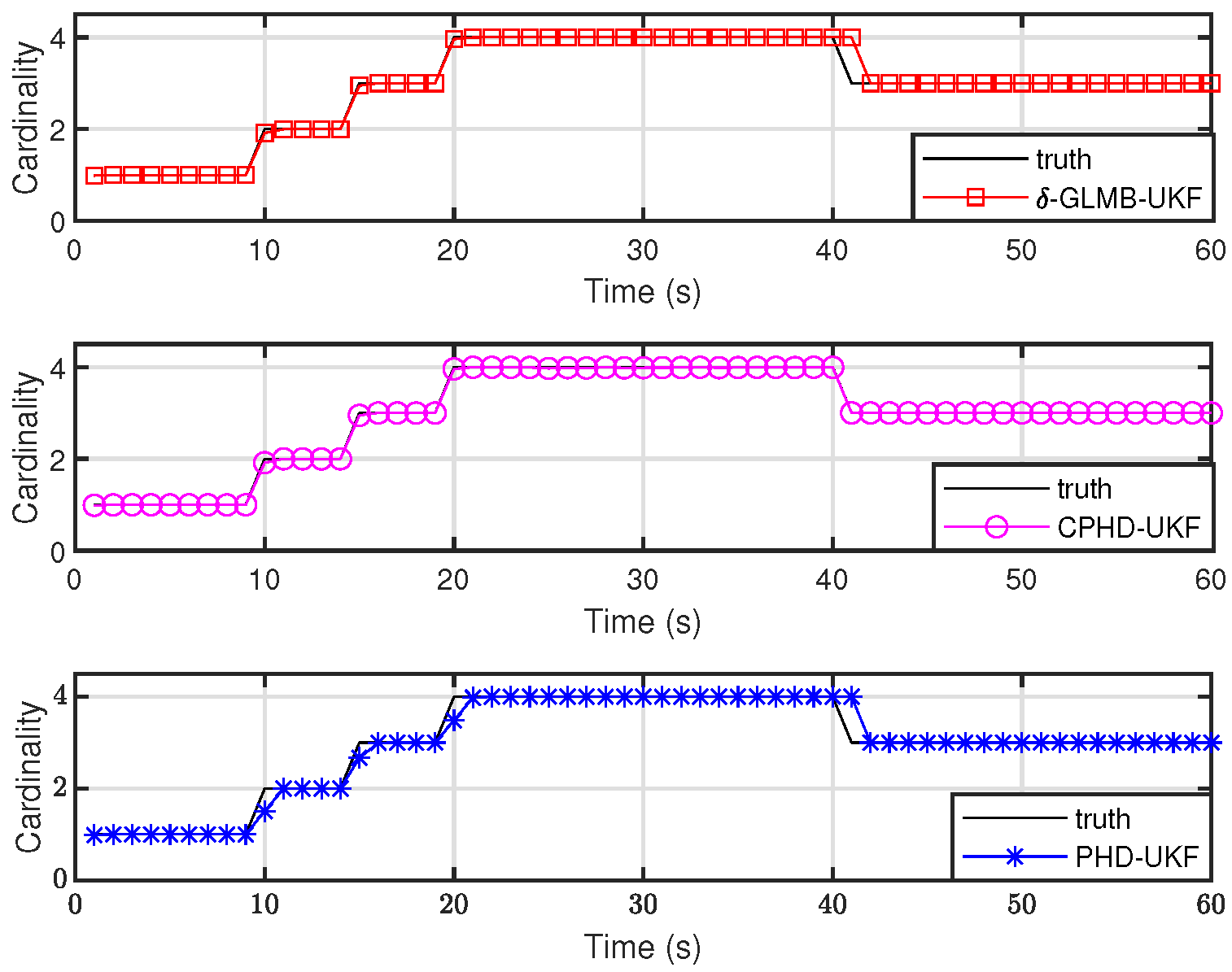
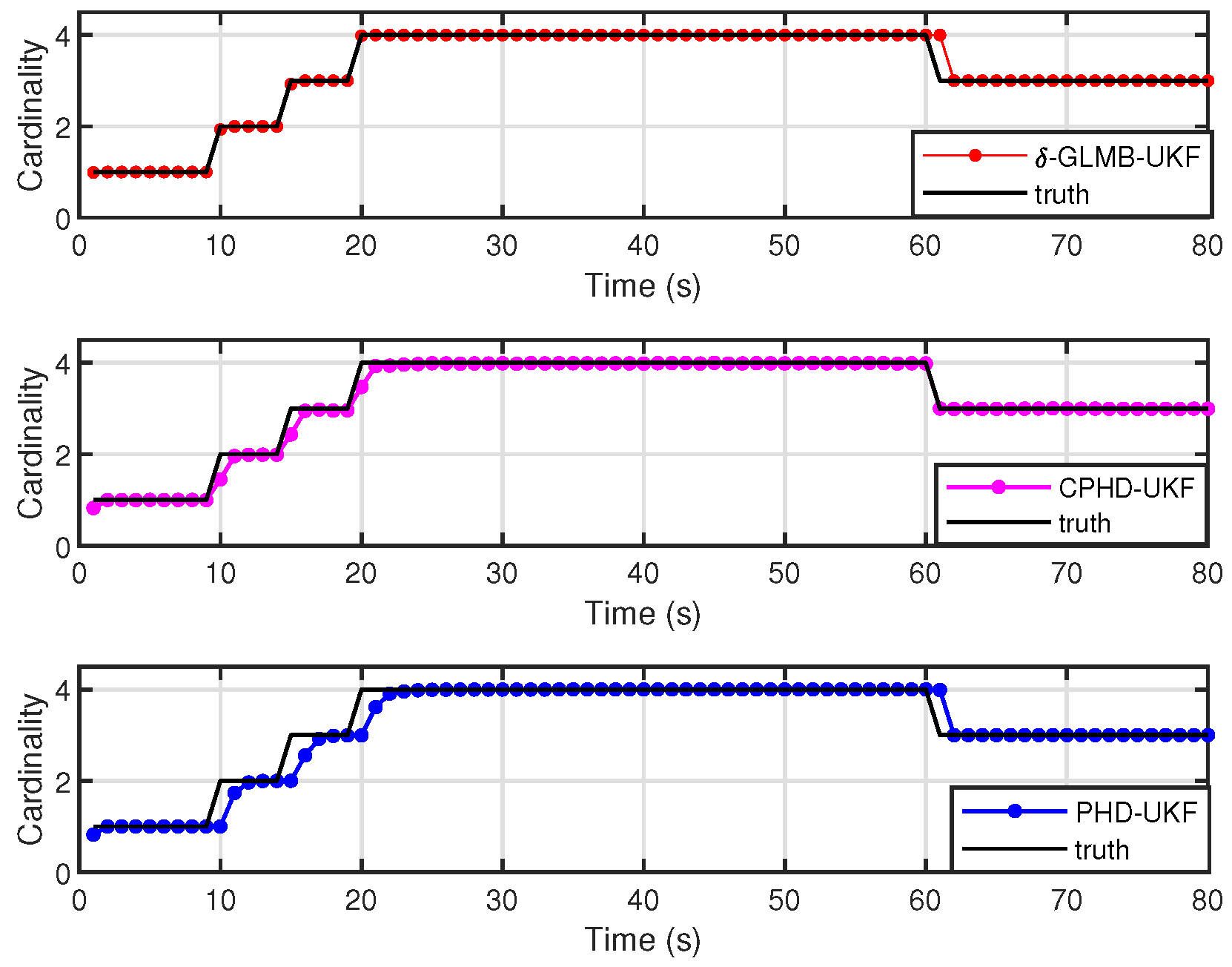
4. Numerical Example

The EKF and UKF recursion implementations of the $\delta$-GLMB filter possess their respective advantages and disadvantages. It is worth noting that both the EKF and UKF approximations are computationally more efficient than the SMC approximation when dealing with nonlinearities. Furthermore, extracting state estimates remains straightforward due to the Gaussian mixture implementation at the core of these methods. In particular, the EKF recursion requires the computation of the Jacobi matrices, limiting its applicability to scenarios where both the state and measurement models are differentiable. In contrast, the UKF recursion avoids the requirement of differentiation altogether and can be applied to the nonlinear model. Therefore, in the subsequent simulation results, we only provide the UKF implementation.

In this section, we conduct two simulation scenarios: stationary and moving BSs. Unfortunately, there is a lack of existing multi-target RFS tracking methods tailored to passive localization and tracking contexts, making direct performance comparisons challenging. Then, we adapt the following established algorithms to the passive localization and tracking context:

• UKF implementation for the PHD filter;
• UKF implementation for the CPHD filter.

We first extend the $\delta$-GLMB filter to the passive localization and tracking scenarios and provide closed-form solutions for both the prediction and update. Compared to the PHD and CPHD filters, the $\delta$-GLMB can provide a multi-target Bayesian filtering solution for target trajectory estimation (i.e., it can recognize the birth information of the tracked target).

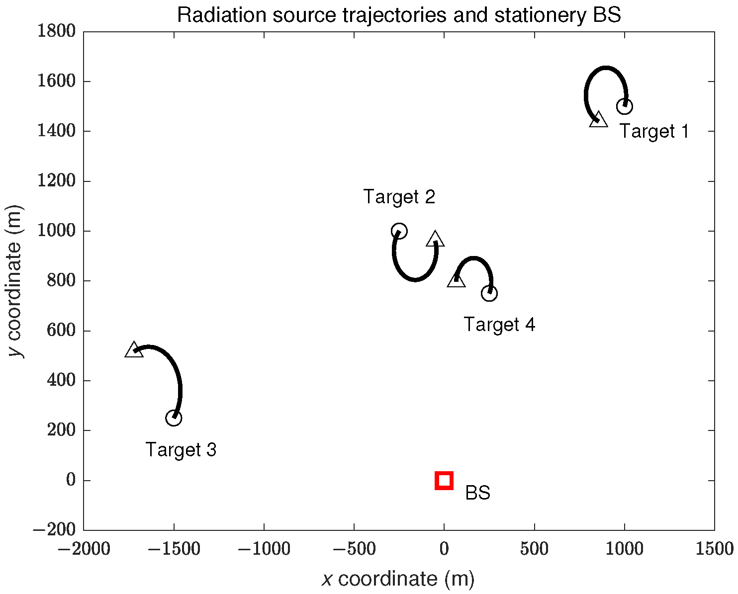
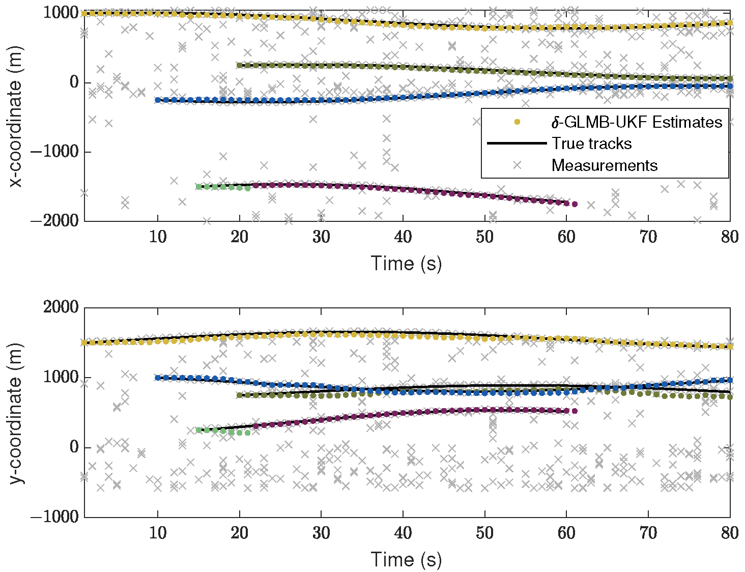
4.1. A Stationary BS for Passive Localization and Tracking

The two-dimensional workspace has a size of $\left[-2000,1500\right]$m $\times \left[-200,1800\right]$m, as illustrated in Figure 3. The number of targets changes over time due to the occurrence of births and deaths. The specific time instances for the births and deaths of the true radiation sources are outlined in

Table 1. Source state.

Source	Survival Time	Initial State ($\mathit{m},\mathit{m}/\mathit{s}$)
1	1–80 s	${\left[997;3;1494;6\right]}^T$
2	10–80 s	${\left[-245;-5;1005;-5\right]}^T$
3	15–60 s	${\left[-1493;-7;242;8\right]}^T$
4	20–80 s	${\left[247;3;745;5\right]}^T$

. The state kinematics equation for the radiation source is

$${\mathbf{x}}_k=\mathbf{F}\left(\varpi \right){\mathbf{x}}_{k-1}+{\Gamma }_k{\mathbf{v}}_{k-1},$$

(75)

and

$$\mathbf{F}\left(\varpi \right)=\left[\begin{array}{cccc}1& \frac{sin\left(\varpi \Delta T\right)}{\varpi }& 0& -\frac{1-cos\left(\varpi \Delta T\right)}{\varpi }\\ 0& cos\left(\varpi \Delta T\right)& 1& -sin\left(\varpi \Delta T\right)\\ 0& \frac{1-cos\left(\varpi \Delta T\right)}{\varpi }& 0& \frac{sin\left(\varpi \Delta T\right)}{\varpi }\\ 0& sin\left(\varpi \Delta T\right)& 0& cos\left(\varpi \Delta T\right)\end{array}\right],$$

(76)

$${\Gamma }_k=\left[\begin{array}{cc}\Delta T^2/\phantom{\Delta T^{2}2}2& 0\\ \Delta T& 0\\ 0& \Delta T^2/\phantom{\Delta T^{2}2}2\\ 0& T\end{array}\right],$$

(77)

where $\Delta T=1s$ and $\varpi =0.06$ rad/s. ${\mathbf{v}}_{k-1}\sim \mathcal{N}\left(·;\mathbf{0},{\mathbf{Q}}_{k-1}\right)$, where ${\mathbf{Q}}_{k-1}=diag\left(\left[1,1\right]\right)$. We assume that the spontaneous newborn model is the LMB RFS with the parameters ${\mathit{\pi }}_B={\left\{r_B^{\left(i\right)},p_B^{\left(i\right)}\right\}}_{i=1}^4$, where $r_B^{\left(1\right)}=r_B^{\left(2\right)}=0.02$, $r_B^{\left(3\right)}=r_B^{\left(4\right)}=,0.03$, and $p_B^{\left(i\right)}\left(\mathbf{x}\right)=\mathcal{N}\left(\mathbf{x};{\mathbf{m}}_B^{\left(i\right)},{\mathbf{P}}_B\right)$, where ${\mathbf{m}}_B^{\left(1\right)}={\left[-1500,0,250,0\right]}^T$, ${\mathbf{m}}_B^{\left(2\right)}={\left[-250,0,1000,0\right]}^T$, ${\mathbf{m}}_B^{\left(3\right)}={\left[250,0,750,0\right]}^T$, ${\mathbf{m}}_B^{\left(4\right)}={\left[1000,0,1500,0\right]}^T$, and ${\mathbf{P}}_B=diag{\left({\left[10,5,10,5\right]}^T\right)}^2$. $P_{S,k}=0.99$, $P_{D,k}=0.90$, $J_{max}=3000$, and $K_B=5$.

If detected, each target generates a noisy azimuth, angular velocity, and Doppler frequency change-rate measurement $\mathbf{z}={\left[{\theta }_k,{\dot{\theta }}_k,{\dot{f}}_k\right]}^T$. The other parameters are ${\delta }_{\theta }^{ }=2\left(\pi /180\right)\mathrm{rad}$, ${\delta }_{\dot{\theta }}^{ }={10}^{-2}\mathrm{rad}/\mathrm{s}$, and ${\delta }_{\dot{f}}^{ }={10}^{-3}\mathrm{Hz}/\mathrm{s}$. The clutter measurements are expected to appear within the range of $\left[-\pi ,\pi \right]\mathrm{rad}\times \left[-\pi /10,\pi /10\right]\mathrm{rad}/\mathrm{s}\times \left[-5,0\right]\mathrm{Hz}/\mathrm{s}$, and the number of clutter obeys a Poisson RFS with a mean value of 5 and an intensity of ${\kappa }_k\left(\mathbf{z}\right)={\lambda }_c\mathcal{U}\left(\mathcal{Z}\right)$, where ${\lambda }_c=5.07\times {10}^{-2}{\left({\mathrm{rad}}^2{\mathrm{Hz}/\mathrm{s}}^2\right)}^{-1}$, and $\mathcal{U}\left(\mathcal{Z}\right)$ denotes the uniform distribution density over the observation region.

The output of the $\delta$-GLMB-UKF filter for one MC run is presented in Figure 4. Notably, although our form of clutter arises from $\left[-\pi ,\pi \right]\mathrm{rad}\times \left[-\pi /10,\pi /10\right]\mathrm{rad}/\mathrm{s}\times \left[-5,0\right]\mathrm{Hz}/\mathrm{s}$, the corresponding $x-y$ coordinates can be derived from Equations (8) and (9). The presence of several clutter interferences at each time moment can be seen in Figure 4, but the $\delta$-GLMB-UKF filter can launch and terminate the tracks with a small delay. We also notice that the estimated trajectory of the third target shows an orbital switch at the 22nd moment, but the newborn labeled target is quickly captured.

We further validate our results by comparing the performance of the $\delta$-GLMB, PHD, and CPHD filters via the UKF implementation. Figure 5 compares the OSPA, [39] distance of the three filters ($p=1$, $c=100$ m) and its localization and cardinality components. As can be seen from Figure 5, the $\delta$-GLMB-UKF filter generally outperforms the other two filters for this scenario, despite the overestimation of the target number at the 61st moment. The cardinality statistics of the three filters are shown in Figure 6 over 500 MC trials. It can be seen from Figure 6 that the $\delta$-GLMB-UKF is superior to the PHD-UKF and CPHD-UKF methods in terms of target number detection.

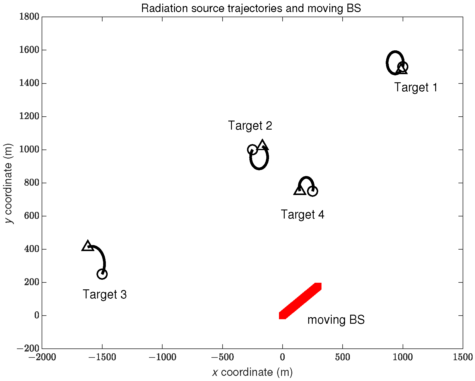
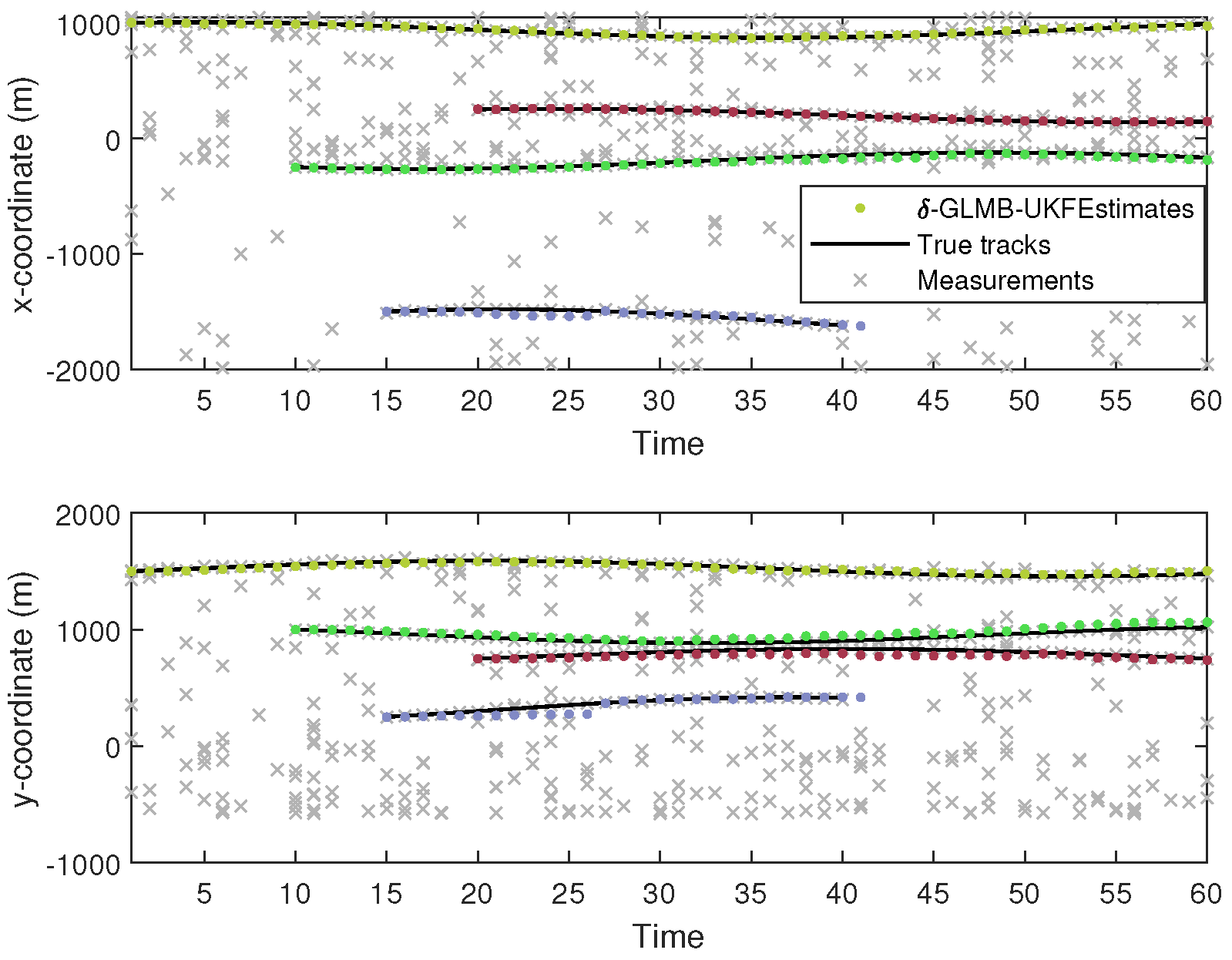
4.2. A Moving BS for Passive Localization and Tracking

Unlike Section 4.1, in this section, the base station is in motion (as depicted in Figure 7), and the duration of this scenario is 60 s. The specific time points of the true radiation sources are provided in

Table 2. Source state.

Source	Survival Time	Initial State ($\mathit{m},\mathit{m}/\mathit{s}$)
1	1–60 s	${\left[997;3;1494;6\right]}^T$
2	10–60 s	${\left[-245;-5;1005;-5\right]}^T$
3	15–40 s	${\left[-1493;-7;242;8\right]}^T$
4	20–60 s	${\left[247;3;745;5\right]}^T$

. The other experimental parameters are consistent with those in Section 4.1.

Figure 8 gives the results of the true and estimated trajectories from the $\delta$-GLMB-UKF filter outputs in the x and y coordinates from one MC trial. Figure 8 shows that the proposed algorithm can still accurately capture the start of the target’s trajectory even in the presence of clutter interference. We also observe that, as expected, although there is no trajectory switching, there is a slight occurrence of lost or spurious trajectories, ensuring that the estimated track identity remains consistent throughout the scenario. Moreover, compared to the trajectory results in Figure 4, the output of the tracked trajectories in the case of the moving base station scenario is more accurate. This is due to the fact that when the base station is moving, we only need to extract the measurement information for time k, which is independent of the base station’s position at the previous $k-1$ moments, thus reducing the data correlation requirements.

Similarly, the cardinality statistics of the three filters over 500 MC trials are shown in Figure 9. Compared to Figure 6, their target number estimation performance is significantly improved. Although $\delta$-GLMB-UKF and PHD-UKF still think that the targets have not disappeared at the 41st moment, the overestimation error is immediately corrected at the 42nd moment. Figure 10 compares the OSPA distances with the localization and base components of the three filters. Figure 10a shows that the $\delta$-GLMB-UKF filter significantly outperforms the PHD-UKF and CPHD-UKF filters. As can be seen from the OSPA cardinality component, the error of the $\delta$-GLMB-UKF method is generally smaller than that of the other two methods for target cardinality estimation (Figure 9 provides a more intuitive representation). The OSPA results for both the localization and cardinality components show that the $\delta$-GLMB-UKF filter outperforms the PHD-UKF and CPHD-UKF filters.

5. Conclusions

This paper explores the application of the $\delta$-GLMB filter in the field of passive localization and tracking of radiation sources. By extending the $\delta$-GLMB filter to the scenario of passive localization and tracking of radiation sources, this paper presents EKF and UKF implementations based on this filter. It provides two simulation cases (stationary base station and moving base station) and tests the UKF implementation of the proposed $\delta$-GLMB, and the simulation results demonstrate the effectiveness of this approach. Moreover, our proposed $\delta$-GLMB-UKF filter accurately tracks the target and captures its trajectory, as demonstrated in simulation examples alongside other filters, thereby verifying the effectiveness of the $\delta$-GLMB filter in target identification and state tracking. Furthermore, the $\delta$-GLMB filter can achieve accurate localization and tracking in complex and dynamic wireless environments, which provides significant theoretical and technical support for enhancing the performance of passive localization and tracking systems for radiation sources and for further research in application areas. In the future, the parameters of the $\delta$-GLMB filter can be further optimized to achieve higher positioning and tracking accuracy. Also, we will consider adding new measurements to the existing trajectories and validating the proposed algorithm in engineering experimental tests.

References

1. Kang, X.; Shao, Y.; Bai, G.; Sun, H.; Zhang, T.; Wang, D. Dual-UAV Collaborative High-Precision Passive Localization Method Based on Optoelectronic Platform. Drones 2023, 7, 646. [Google Scholar] [CrossRef]
2. Torrieri, D.J. Statistical theory of passive location systems. IEEE Trans. Aerosp. Electron. Syst. 1984, 2, 183–198. [Google Scholar] [CrossRef]
3. Wang, J.; Du, H.; Niyato, D.; Zhou, M.; Kang, J.; Xiong, Z.; Jamalipour, A. Through the Wall Detection and Localization of Autonomous Mobile Device in Indoor Scenario. IEEE J. Sel. Areas Commun. 2024, 42, 161–176. [Google Scholar] [CrossRef]
4. Xiang, F.; Wang, J.; Yuan, X. Research on passive detection and location by fixed single observer. In Proceedings of the 2020 International Conference on Information Science, Parallel and Distributed Systems (ISPDS), Xi’an, China, 14–16 August 2020; pp. 35–39. [Google Scholar]
5. Shen, J.; Molisch, A.F.; Salmi, J. Accurate passive location estimation using TOA measurements. IEEE Trans. Wirel. Commun. 2012, 11, 2182–2192. [Google Scholar] [CrossRef]
6. Weiss, A.J. On the accuracy of a cellular location system based on RSS measurements. IEEE Trans. Veh. Technol. 2003, 52, 1508–1518. [Google Scholar] [CrossRef]
7. Guvenc, I.; Chong, C.C. A survey on TOA based wireless localization and NLOS mitigation techniques. IEEE Commun. Surv. Tutor. 2009, 11, 107–124. [Google Scholar] [CrossRef]
8. Chen, R.; Long, W.X.; Wang, X.; Jiandong, L. Multi-Mode OAM Radio Waves: Generation, Angle of Arrival Estimation and Reception With UCAs. IEEE Trans. Wirel. Commun. 2020, 19, 6932–6947. [Google Scholar] [CrossRef]
9. Zhang, W.; Zhu, X.; Zhao, Z.; Liu, Y.; Yang, S. High accuracy positioning system based on multistation UWB time-of-flight measurements. In Proceedings of the 2020 IEEE International Conference on Computational Electromagnetics (ICCEM), IEEE, Singaproe, 24–26 August 2020; pp. 268–270. [Google Scholar]
10. Garraffa, G.; Sferlazza, A.; D’Ippolito, F.; Alonge, F. Localization Based on parallel robots Kinematics As an Alternative to Trilateration. IEEE Trans. Ind. Electron. 2021, 69, 999–1010. [Google Scholar] [CrossRef]
11. Mahler, R.P. Statistical Multisource-Multitarget Information Fusion; Artech House: Norwood, MA, USA, 2007; Volume 685. [Google Scholar]
12. Jeong, T.T. Particle PHD filter multiple target tracking in sonar image. IEEE Trans. Aerosp. Electron. Syst. 2007, 43, 409–416. [Google Scholar] [CrossRef]
13. Pham, N.T.; Huang, W.; Ong, S.H. Tracking multiple objects using probability hypothesis density filter and color measurements. In Proceedings of the 2007 IEEE International Conference on Multimedia and Expo, Beijing, China, 2–5 July 2007; pp. 1511–1514. [Google Scholar]
14. Hoseinnezhad, R.; Vo, B.N.; Vo, B.T. Visual tracking in background subtracted image sequences via multi-Bernoulli filtering. IEEE Trans. Signal Process. 2012, 61, 392–397. [Google Scholar] [CrossRef]
15. Canaud, M.; Mihaylova, L.; Sau, J.; El Faouzi, N.E. Probabilty hypothesis density filtering for real-time traffic state estimation and prediction. Netw. Heterog. Media (NHM) 2013, 8, 825–842. [Google Scholar] [CrossRef]
16. Zhang, X. Adaptive control and reconfiguration of mobile wireless sensor networks for dynamic multi-target tracking. IEEE Trans. Autom. Control. 2011, 56, 2429–2444. [Google Scholar] [CrossRef]
17. Battistelli, G.; Chisci, L.; Fantacci, C.; Farina, A.; Graziano, A. Consensus CPHD filter for distributed multitarget tracking. IEEE J. Sel. Top. Signal Process. 2013, 7, 508–520. [Google Scholar] [CrossRef]
18. Ueney, M.; Clark, D.E.; Julier, S.J. Distributed fusion of PHD filters via exponential mixture densities. IEEE J. Sel. Top. Signal Process. 2013, 7, 521–531. [Google Scholar] [CrossRef]
19. Mahler, R.P. Multitarget Bayes filtering via first-order multitarget moments. IEEE Trans. Aerosp. Electron. Syst. 2003, 39, 1152–1178. [Google Scholar] [CrossRef]
20. Lindenmaier, L.; Aradi, S.; Bécsi, T.; Törő, O.; Gáspár, P. GM-PHD Filter Based Sensor Data Fusion for Automotive Frontal Perception System. IEEE Trans. Veh. Technol. 2022, 71, 7215–7229. [Google Scholar] [CrossRef]
21. Tian, Y.; Liu, M.; Zhang, S.; Zheng, R.; Dong, S.; Liu, Z. Underwater Target Tracking Based on the Feature-Aided GM-PHD Method. IEEE Trans. Instrum. Meas. 2024, 73, 5500412. [Google Scholar] [CrossRef]
22. Mahler, R. PHD filters of higher order in target number. IEEE Trans. Aerosp. Electron. Syst. 2007, 43, 1523–1543. [Google Scholar] [CrossRef]
23. Wei, S.; Zhang, B.; Yi, W. Trajectory PHD and CPHD Filters With Unknown Detection Profile. IEEE Trans. Veh. Technol. 2022, 71, 8042–8058. [Google Scholar] [CrossRef]
24. Vo, B.T.; Vo, B.N.; Cantoni, A. The cardinality balanced multi-target multi-Bernoulli filter and its implementations. IEEE Trans. Signal Process. 2008, 57, 409–423. [Google Scholar]
25. Davies, E.S.; García-Fernández, A.F. Information Exchange Track-Before-Detect Multi-Bernoulli Filter for Superpositional Sensors. IEEE Trans. Signal Process. 2024, 72, 607–621. [Google Scholar] [CrossRef]
26. Vo, B.T.; Vo, B.N. Labeled Random Finite Sets and Multi-Object Conjugate Priors. IEEE Trans. Signal Process. 2013, 61, 3460–3475. [Google Scholar] [CrossRef]
27. Wu, W.; Sun, H.; Cai, Y.; Jiang, S.; Xiong, J. Tracking Multiple Maneuvering Targets Hidden in the DBZ Based on the MM-GLMB Filter. IEEE Trans. Signal Process. 2020, 68, 2912–2924. [Google Scholar] [CrossRef]
28. Wu, W.; Sun, H.; Cai, Y.; Xiong, J. MM-GLMB Filter-Based Sensor Control for Tracking Multiple Maneuvering Targets Hidden in the Doppler Blind Zone. IEEE Trans. Signal Process. 2020, 68, 4555–4567. [Google Scholar] [CrossRef]
29. Vo, B.N.; Vo, B.T.; Phung, D. Labeled Random Finite Sets and the Bayes Multi-Target Tracking Filter. IEEE Trans. Signal Process. 2014, 62, 6554–6567. [Google Scholar] [CrossRef]
30. Liu, Z.; Gan, J.; Li, J.; Wu, M. Adaptive δ-Generalized Labeled Multi-Bernoulli Filter for Multi-Object Detection and Tracking. IEEE Access 2021, 9, 2100–2109. [Google Scholar] [CrossRef]
31. Shim, C.; Vo, B.T.; Vo, B.N.; Ong, J.; Moratuwage, D. Linear Complexity Gibbs Sampling for Generalized Labeled Multi-Bernoulli Filtering. IEEE Trans. Signal Process. 2023, 71, 1981–1994. [Google Scholar] [CrossRef]
32. Vo, B.N.; Vo, B.T.; Beard, M. Multi-Sensor Multi-Object Tracking With the Generalized Labeled Multi-Bernoulli Filter. IEEE Trans. Signal Process. 2019, 67, 5952–5967. [Google Scholar] [CrossRef]
33. Vo, B.N.; Vo, B.T. A Multi-Scan Labeled Random Finite Set Model for Multi-Object State Estimation. IEEE Trans. Signal Process. 2019, 67, 4948–4963. [Google Scholar] [CrossRef]
34. Nguyen, T.T.D.; Vo, B.N.; Vo, B.T.; Kim, D.Y.; Choi, Y.S. Tracking Cells and Their Lineages Via Labeled Random Finite Sets. IEEE Trans. Signal Process. 2021, 69, 5611–5626. [Google Scholar] [CrossRef]
35. Van Nguyen, H.; Rezatofighi, H.; Vo, B.N.; Ranasinghe, D.C. Distributed multi-object tracking under limited field of view sensors. IEEE Trans. Signal Process. 2021, 69, 5329–5344. [Google Scholar] [CrossRef]
36. Dong, X.; Zhao, J.; Sun, M.; Zhang, X.; Wang, Y. A Modified δ-Generalized Labeled Multi-Bernoulli Filtering for Multi-Source DOA Tracking with Coprime Array. IEEE Trans. Wirel. Commun. 2023, 22, 9424–9437. [Google Scholar] [CrossRef]
37. Kuhn, H.W. The Hungarian method for the assignment problem. Nav. Res. Logist. Q. 1955, 2, 83–97. [Google Scholar] [CrossRef]
38. Murty, K.G. An algorithm for ranking all the assignments in order of increasing cost. Oper. Res. 1968, 16, 682–687. [Google Scholar] [CrossRef]
39. Schuhmacher, D.; Vo, B.T.; Vo, B.N. A Consistent Metric for Performance Evaluation of Multi-Object Filters. IEEE Trans. Signal Process. 2008, 56, 3447–3457. [Google Scholar] [CrossRef]
Figure 1. The passive localization model between the moving BS and multi-radiation sources carried by UAVs.
Drones 08 00096 g001
Figure 2. The directed graph comprises nodes l 1 , , l I along with their associated cost function values c I , ϑ l 1 , , c I , ϑ l I . Here, S and E denote the starting and ending nodes, respectively.
Drones 08 00096 g002
Figure 3. Multi-target trajectories. The start/stop positions of each trajectory are denoted as o / △, and the stationery BS is denoted as □ in red.
Drones 08 00096 g003
Figure 4. Estimated and truth trajectories.
Drones 08 00096 g004
Figure 5. The OSPA distance, localization, and cardinality ( p = 1 , c = 100 m) for the δ -GLMB-UKF, CPHD-UKF, and CPHD-UKF filters. (a) OSPA distance; (b) OSPA localization; (c) OSPA cardinality.
Drones 08 00096 g005
Figure 6. Cardinality for the δ -GLMB-UKF, CPHD-UKF, and CPHD-UKF filters versus time.
Drones 08 00096 g006
Figure 7. Multi-target trajectories on the plane. The start/stop positions of each trajectory are denoted as o / △, and the moving BS is denoted as □ in red.
Drones 08 00096 g007
Figure 8. Estimated and truth trajectories for x y coordinates versus time.
Drones 08 00096 g008
Figure 9. Cardinality for the δ -GLMB-UKF, CPHD-UKF, and CPHD-UKF filters versus time.
Drones 08 00096 g009
Figure 10. The OSPA distance, localization, and cardinality ( p = 1 , c = 100 m) for the δ -GLMB-UKF, CPHD-UKF, and CPHD-UKF filters. (a) OSPA distance; (b) OSPA localization; (c) OSPA cardinality.
Drones 08 00096 g010