Abstract
Monitoring and mapping crop water stress and variability at a farm scale for cereals such as maize, one of the most common crops in developing countries with 200 million people around the world, is an important objective within precision agriculture. In this regard, unmanned aerial vehicle-obtained multispectral and thermal imagery has been adopted to estimate the crop water stress proxy (i.e., Crop Water Stress Index) in conjunction with algorithm machine learning techniques, namely, partial least squares (PLS), support vector machines (SVM), and random forest (RF), on a typical smallholder farm in southern Africa. This study addresses this objective by determining the change between foliar and ambient temperature (Tc-Ta) and vapor pressure deficit to determine the non-water stressed baseline for computing the maize Crop Water Stress Index. The findings revealed a significant relationship between vapor pressure deficit and Tc-Ta (R2 = 0.84) during the vegetative stage between 10:00 and 14:00 (South Africa Standard Time). Also, the findings revealed that the best model for predicting the Crop Water Stress Index was obtained using the random forest algorithm (R2 = 0.85, RMSE = 0.05, MAE = 0.04) using NDRE, MTCI, CCCI, GNDVI, TIR, Cl_Red Edge, MTVI2, Red, Blue, and Cl_Green as optimal variables, in order of importance. The results indicated that NIR, Red, Red Edge derivatives, and thermal band were some of the optimal predictor variables for the Crop Water Stress Index. Finally, using unmanned aerial vehicle data to predict maize crop water stress index on a southern African smallholder farm has shown encouraging results when evaluating its usefulness regarding the use of machine learning techniques. This underscores the urgent need for such technology to improve crop monitoring and water stress assessment, providing valuable insights for sustainable agricultural practices in food-insecure regions.
1. Introduction
Maize (Zea mays L.) is one of the most crucial crops and a primary food source for approximately 4.5 billion people in 95 developing countries, including southern African countries [1]. At the same time, maize is one of the globe’s crops affected by drought and heat stress because of a lack of precipitation due to climate change [2]. In particular, the limited availability of water adversely affects maize metabolic activities, limiting biomass accumulation and decreasing photosynthetic rates due to reduced chlorophylls in leaves, ultimately leading to lower yields [3]. Risks linked with precipitation variability could threaten national food security in developing southern African countries, considering the significance of maize production for local supply in these regions [4]. As a result, water stress quantification has become an essential issue for agricultural production, in particular precision farming. In order to support the design and adaptation of climate change mitigation and adaptation measures, it is particularly important to unravel spatiotemporal patterns and the severity of water stress at different scales [5]. Soil-based methods have traditionally been the primary means of assessing crop water stress; however, there has been an increasing preference for plant-based methods. The indirect assessment of the actual plant water status, as highlighted by [6], makes this method less preferred. Plant-based methods offer a more direct proxy for crop water’s actual state than soil-based methods [7].
Evaluating crop canopy temperature variations as a proxy for water status is one of the most widely used plant-based methods. Researchers have investigated canopy temperature as a water stress indicator based on its inverse relationship with the rate of water loss and stomatal behaviour [8]. This is because when the heat is absorbed into the crop, the temperature of the crop canopy increases, but it cools when the heat is used to evaporate water or transpire. The stomata close in response to soil water depletion, leading to decreased water uptake, gas exchange, and photosynthesis [6]. Thus, water-stressed plants would generally have less transpiration and thus higher temperatures than those not affected by the stress [8,9,10].
Canopy temperature variations are often quantified using imagers and thermal infrared thermometers [11]. Hand-held thermometers were developed and gained popularity in the 1970s and 1980s [12,13], leading to the establishment of the Crop Water Stress Index (CWSI). This normalised index has been developed to overcome the effects of other environmental parameters that significantly alter the relationship between plant stress and plant temperature [8]. CWSI ranges between 0 and 1, representing a continuum from no water stress to water stress [12,13]. The premise behind the index computation is detailed in the work of [13]. To provide an early intervention in increasing crop production, the CWSI could be used to identify water-stressed crops. In this regard, the CWSI, based on the surface temperature of the canopy, is now considered the preferred index for quantifying water stress in crops [14]. The literature shows that this range is consistent with stress levels in many crops [8] which include grapes [15], olive [8,16], nectarine [17], peach [18], potatoes [19,20], sunflower [21,22], African eggplant [23], and wheat [24].
Furthermore, the empirical CWSI approach makes it necessary to use a non-water-stressed baseline (NWSB) generated from the linear relationship between canopy and air temperature difference (Tc-Ta) for well-watered crops and vapor pressure deficit (VPD) to calculate the lower limit. For a given combination of crop and environmental conditions, this relationship is consistent [6]. It is important to highlight that the CWSI has been effectively implemented in determining maize water stress across various climatic conditions. Studies in China [25,26], the United States of America [27,28], and Thailand [6,29] have successfully implemented the CWSI for this purpose. While CWSI has been widely utilised globally to assess maize water stress, there is still a need to further explore its applicability in Africa, especially in southern Africa, where a decline in maize production has been observed [4,30]. Above all, very few studies have explicitly assessed the maize CWSI in smallholder croplands of southern African environmental conditions.
Meanwhile, incorporating remote sensing techniques into precision agriculture has revealed numerous methods conducive to spatially characterizing the CWSI explicitly for critical crops such as maize. A remote measurement capability eliminates the need for labour-intensive and time-consuming techniques traditionally used to detect water stress at the field or farm level. This efficiency in data collection and stress assessment is a significant advantage and a driving force behind the interest in utilising the CWSI for optimising crop production. However, the utility of remote sensing, particularly in regions like southern Africa, has been hindered by the scarcity of data suitable for field-scale applications. Freely available satellite remotely sensed data (i.e., Landsat TM, ASTER, or MODIS) are typically characterized by coarse spatial resolutions, which are not suitable for accurately capturing canopy temperature variations of different crops against the soil background in heterogeneous smallholder croplands [31,32].
Furthermore, cloud cover remains an important challenge with the use of satellites relaying remote sensing data [33]. Recently, to create a highly spatiotemporally precise platform to specifically detect and monitor water stress in crops, UAVs have evolved a popularly functioning system that delivers remotely sensed data that is relevant for spatial awareness [8,34]. In particular, temperature-based imagery acquired through UAV-borne platforms can efficiently capture crop water stress by analysing canopy temperature concerning the physiological parameters of a crop at a field scale [35]. Several studies have shown a strong relationship between CWSI data derived from UAVs and physiology parameters, e.g., transpiration rates, stomatal conductance, leaf water potential, or stem water potential, in crops like maize [15,26].
Furthermore, regarding the aspect of UAV remotely sensed data’s spatial resolution, several studies have illustrated that spectral derivatives exhibit superior performance compared to conventional bands in mapping crop attributes [36,37]. In the plant canopy, vegetation indexes can detect minute changes [38] because they significantly correlate with water stress indicators such as stomatal conductance [39,40]. In the case of [39], a large correlation between NDVI and stem water potential was identified with an R2 value of 0.68. On the other hand, results obtained by [41] revealed a significant relationship between stomatal conductance and GNDVI (p < 0.01). Ref. [42] found a correlation of R2 = 0.77 between the normalised photochemical reflectance index (PRInorm) and CWSI. Ref. [31] developed CWSI inversion models based on vegetation indices that showed the best relationship with CWSI, TCARI/RDVI, and TCARI/SAVI (both with an R2 value greater than 0.80). More efforts are required to document the relationship between UAV multispectral vegetation indices and CWSI, particularly for the maize crops in smallholder croplands.
Moreover, various machine learning methods, such as RFs, SVMs, and ANNs, were widely employed and demonstrated to be accurate and effective in detecting and mapping various crop attributes, including water stress [37,43,44,45,46]. Because they use sophisticated statistical techniques, machine learning methods are the most precise and effective methods to learn complex non-linear functions between spectral data and biophysical parameters [47]. For instance, Ref. [48] established that the RF algorithm was best for estimating maize’s specific leaf area, equivalent water thickness, and fuel moisture content to rRMSEs of 3.48%, 3.13%, and 1%, respectively. RF has been applied to predict the CWSI for crops other than maize [49,50,51]. For instance, Ref. [51] demonstrated that RF could optimally estimate the CWSI of B. chinensis var. parachinensis (R2 = 0.86). Ref. [50] observed that RF outperformed SVM in estimating chlorophyll content, with average RMSEs of 2.90 and 3.11, respectively. However, SVM has also shown promising results in predicting relative water content, achieving an R2 of 0.72 and an RMSE of 6.22% [49]. Nonetheless, the literature also shows that, despite the optimum performance of these machine learning algorithms, no algorithm has been exhaustively tested to enable the accurate and effective identification and mapping of plant characteristics in a variety of environments [52,53]. Additionally, very few studies have sought to characterise the maize CWSI using UAV-acquired data. Therefore, the efficiency of different commonly used machine learning approaches in predicting the CWSI needs to be further assessed.
Therefore, the objective of this study was to conduct a comparative assessment of the performance of PLSR, SVM, and RF in estimating the maize CWSI using UAV-acquired remotely sensed data in smallholder croplands typically found in southern Africa. To address this objective, the relative contribution of bands, vegetation indices, and both datasets combined was evaluated. This research sought to provide a reference to accurately capture the spatiotemporal characteristics of the CWSI in the typical small-scale agricultural areas of developing countries in southern Africa. The study established a maize Crop Water Stress Index based on field temperature data to achieve this overall objective. The significance of this study lies in its addressing a critical aspect of precision agriculture, which is leveraging advanced technologies and analytical methods for the near-real-time monitoring and mapping of the maize crop water stress, in the context of smallholder farms in developing countries, specifically for optimising food production. The findings of this study will have implications for sustainable agriculture and food security in regions facing water-related issues.
2. Materials and Methods
2.1. Study Site
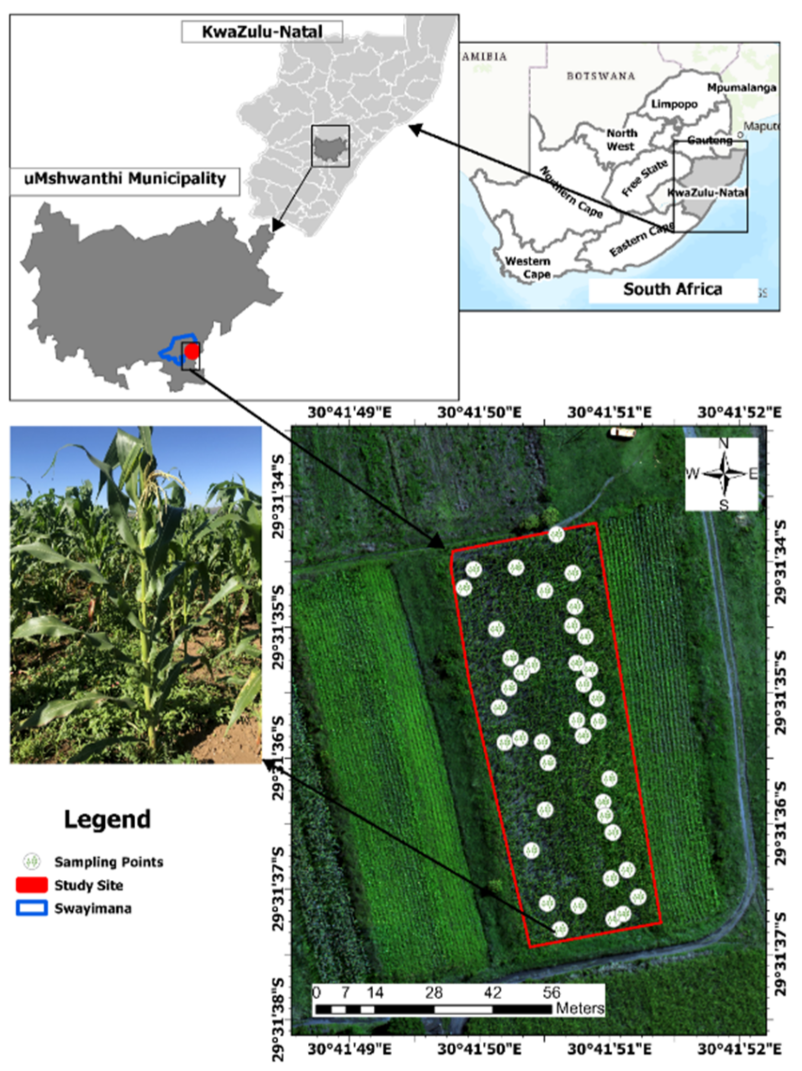
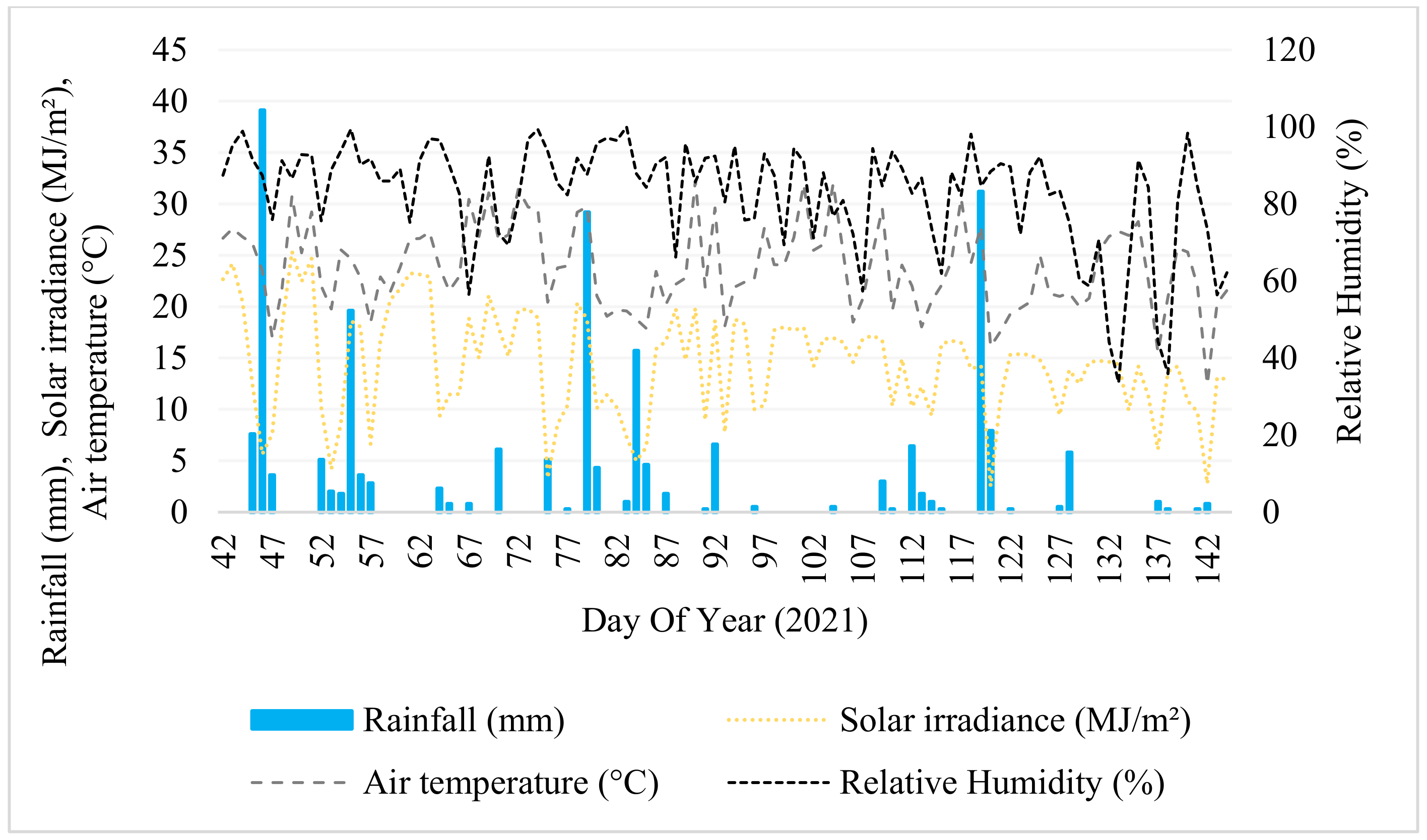
This study was conducted at the rural area of Swayimana, uMshwathi Local Municipality, approximately 55 km north-east of Pietermaritzburg, in the KwaZulu-Natal Province, South Africa (−22.125031° to −34.834171° S and 16.451891° to 32.891122° E) (Figure 1). The area is dominated by smallholder farming systems with dominant rain-fed crops such as sugarcane, maize, sweet potato, and amadumbe (taro). The climate is mainly warm and wet in summer and dry in winter. The mean annual temperature is 17 °C, ranging between 11.8 °C and 24 °C. The mean annual rainfall varies between 600 and 1200 mm, with most of it coming during the summer. During the study period, the area received an average of 242.8 mm rainfall, 82.81% humidity, and a maximum average air temperature of 24 °C (Figure 2). These measurements were taken using an Automatic Weather Station installed at a school, following the World Meteorological Organization’s standards, proximal to the study area. This research was carried out in an area of 0.28 hectares farmed with smallholder maize (Figure 1).

Figure 1.
Location of the Swayimana study area, study site, and smallholder maize field.
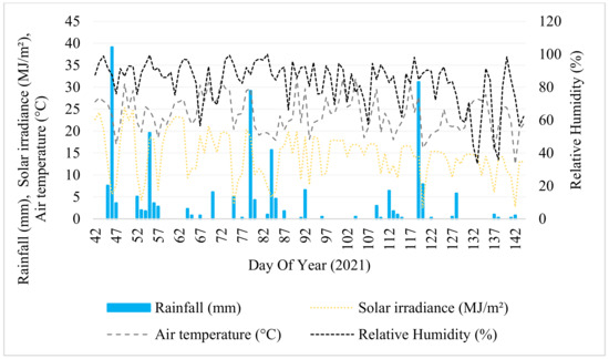
Figure 2.
Swayimana weather conditions over the study period.
2.2. Maize Canopy Temperature Measurement
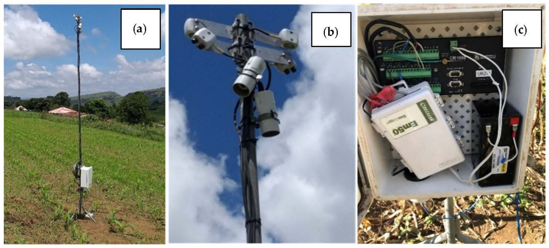
The maize was sown on 8 February 2021 and harvested on 26 May 2021. At the centre of the maize field, two infrared radiometers (IRRs; SI-111, Apogee Instruments Inc., Logan, UT, USA), mounted on a four-meter meteorological tower, were installed (Figure 3b). In the range of −60 °C to 110 °C, the sensor measured the target temperature at 8–14 m. The surface temperature was measured in a 23 and 45 half angle field of view (FOV) perpendicular to the direction of the row. Using the CR1000 datalogger (Campbell Scientific, Logan, UT, USA), temperatures were measured 10 s apart and averaged to 5 min, 10 min, 30 min, and 60 min (Figure 3c). The 10:00–14:00 (South Africa Standard Time) 60 min foliar temperature data were used in this study to develop the daily vapor pressure deficit (VPD) and vapor pressure gradient (VPG), and ultimately the non-water-stressed baseline (NWSB) and non-transpiring baseline (NTB).

Figure 3.
(a) Automated in-field meteorological tower in the maize field, (b) meteorological tower-mounted infrared radiometers (IRRs), and (c) CR1000 data logger, Em50 datalogger, and 12 V battery [54].
A temperature-controlled room with blackbody cones was used for the radiation source calibration of IRR sensors. To do so, sensors were placed within the fitting when the blackbody cone was opened. The thermal isolation of IRR sensors from the cones was used to ensure that each one could measure its temperature. The IRRs did not change, while the cone was monitored and noted to be at temperatures under 12 °C and above 18 °C in addition to a temperature level equal to or less than that of the IRRs. From every 10 °C, measurements of the IRRs and blackbody cones were taken until they reached constant temperatures. IRR measurements on maize temperature were carried out to calibrate hand-held IRT measurements to develop the CWSI.
A polygon in the experimental field was digitised in the Google Earth Pro domain and imported into ArcGIS 10.5 to generate sample points. In the digitised field boundary, a total of 50 sample points were generated based on stratified random sampling. These points were then uploaded into a hand-held Trimble Global Positioning System (GPS) with sub-meter accuracy. These GPS points were used to navigate to the actual sampling point in the field. Maize plants that coincided with or were within proximity to the point were considered for temperature measurements in this study. For consistent biweekly measurements, maize plants were marked at each sampling point. Specifically, 50 maize points were sampled four times across the growing season.
The temperature of the maize, from the early vegetative growth stage to the late reproductive growth stage, was measured with a hand-held infrared GM320 IRT thermometer, using a digital laser, at two weekly intervals. Infrared thermometers (IRTs) with the capability of recording temperatures ranging from approximately −50 °C to 330 °C were used to measure maize canopy temperatures in the field. These measurements were carried out concurrently with the UAV image acquisition, between 11:00 a.m. and 2:00 p.m. (South Africa Standard Time). IRT values from the vegetative and tasselling stages were obtained from the most recent completely grown leaf with an open collar. After that, measurements were taken at the same node as the primary ear shank, where an ear leaf is attached [55]. At each sampling point, the IRT was held at about 2 m above the ground and approximately 50 cm from the canopy. Three subsequent temperature measurements were taken to ensure that a maize canopy dominated the fields of view. The temperature measurements were captured along with each plant’s location. Subsequently, a point map with this information was produced in a GIS and later used to extract the crop spectral signatures for statistical analysis.
2.3. Meteorological Data Collection
The automatic weather station (AWS) was used for the meteorological data. Hourly averaged meteorological data comprising air temperature (°C), wind speed (m/s), solar radiation (Wm−2), and relative humidity (%) were used. The following temperature and relative humidity sensors were used to observe meteorological variables above ground: CS215 Temp/RH probe (temperature and relative humidity) and Licor LI2005 pyranometer (solar radiation).
2.4. Crop Water Stress Index (CWSI) Calculation
While alternative approaches, such as soil moisture methods and the measurement of temperature and stomatal conductance demonstrated by [54], exist, the Crop Water Stress Index (CWSI) stands out as one of the proxies that can be effectively correlated with the direct detection and mapping of water stress in maize crops. The CWSI was calculated using calibrated foliar temperature data measured using a hand-held infrared thermometer (IRT) detailed in Section 2.2 and data measured using the AWS. Specifically, the CWSI was calculated by using (1):
where ΔT, Twet, and Tdry are the actual measurements of the difference between the canopy and air temperature (Tc − Ta), lower limit, and upper limit of baselines estimated, respectively. The upper and lower limits are also, respectively, referred to as NWSB and non-transpiring baseline (NTB), and are calculated as follows (2) and (3):
where m and b represent the slope and intercept, respectively. VPD represents vapour pressure deficit, and is calculated using (4)–(6) by relating it to air temperature (Ta) and relative humidity (RH) collected from the field station, following the description of [55]:
where T, RH, , and are the air temperature, relative humidity, saturated vapor pressure (kPa) at the air temperature Ta, and actual vapor pressure (kPa), respectively. As mentioned above, the weather data were measured using the AWS. To calculate Tdry values, the vapour pressure gradient (VPG) was determined. VPG is the change in the pressure of the air-saturated water vapour at the temperature (Ta) and the pressure of the air-saturated water vapour at the temperature (Ta + b) [26].
The first step to determine the CWSI involved determining functions for Twet and Tdry for rainfed maize in Swayimana environmental conditions. This was achieved by following the procedure outlined in [56]. After two significant rainfall days, maize ΔT was collected using the IRT sensors in the field and plotted with their respective VPD values. This assumes that the soil water deficit was remedied because of these wet spells, which led to maize having access to adequate soil water. Therefore, conditions existed that were not water-stressed. This was determined for 2 h before and 2 h after midday, as recommended in [12]. The resulting equation from this linear segment was extracted to obtain the coefficients of (2) and (3). by using simple linear regression. A three-step moving average was followed to plot the relationship between ΔT and VPD, as [13] suggested. According to [56], the CWSI method is valid only when the conditions of clarity are met, to ensure that all the days selected to calculate the CWSI correspond to the field visit days. CWSI values range from 0 to 1, with 0 indicating no water stress and 1 indicating the most severe stress. In addition, a relationship between foliar temperature and stomatal behaviour has been observed during the maize phenological cycle [54]. To illustrate the relationship between water consumption and the foliar temperature used to calculate the CWSI in this study, additionally, the CWSI was computed for four phenological stages.
2.5. UAV Multispectral–Thermal System
A DJI Matrice 300 (DJI Inc., Shenzhen, China) quad-rotor UAV and Micasense (MicaSense, Inc., Seattle, WA, USA) multispectral sensor covering the RGB, NIR, Red Edge, and thermal sections of the electromagnetic spectrum was used to collect images in this study (Figure 4b). The MicaSense has a Downwelling Light Sensor 2 (DLS-2) and MicaSense Altum camera to capture images from a platform of a low-altitude UAV camera system over the smallholder farms. The MicaSense Altum camera has five high-resolution multispectral narrow bands (blue, green, red, red-edge, and NIR) and a radiometric longwave infrared thermal camera. The spectral characteristics of the MicaSense are detailed in Table 1 [48,54].
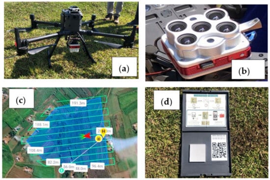
Figure 4.
(a) UAV system, DJI Matrice 300, and (b) MicaSense Altum camera. (c) DJI M-300 flight plan. (d) MicaSense Altum calibration reflectance (CRP) panel.

Table 1.
MicaSense Altum camera specifications [54].
2.6. Image Acquisition and Processing
A kml file representing the boundary of the maize field digitised in Google Earth Pro was used to develop the flight plan. This was transferred into the DJI controller’s intelligent console and used to create flight plans (Figure 4c). The MicaSense Altum sensor was calibrated before and after the flight using a calibration reflectance panel (CRP) (Figure 4d). Users had to manually take an unshaded picture directly over the CRP to determine the illumination conditions for a particular flight day, time, and location. The UAV was flown in the clearest air conditions every two weeks, between 10:00 and 14:00. This period was concurrent with canopy temperature measurements. Detailed flight conditions are presented in the works of [48,54].
After 3576 images were acquired, they were stitched together and radiometrically corrected using Pix4Dfields software 1.8.0 (Pix4d Inc., San Francisco, CA, USA). While the exact details of radiometric correction in Pix4d may be proprietary, the general workflow involves utilising CRP images captured before and after the flight to administer radiometric and atmospheric correction to a MicaSense multispectral image. It applies sensor-specific calibration parameters to normalise the digital number values. It then implements dark object subtraction (DOS) to identify and subtract the dark objects based on the CPR images. This corrects for sensor biases and atmospheric scattering. Then, histogram matching is implemented to standardise the distribution of pixel values across the bands. The CPR images are also used as a white reference for adjusting potential variations in illumination conditions, ensuring pixel values are normalised to a standard reflectance scale. After processing, Pix4d generates a complete orthomosaic and digital elevation model (DEM) as GeoTiff images. Using Google Earth Pro, ground reference points were digitised to core-register the orthomosaic image in ArcGIS 10.5. Images were referenced to the Universal Transverse Mercator (UTM zone 36S) projection after attaining RMSE less than half a pixel (3.5 cm). The image was then used to compute vegetation indices.
2.7. Vegetation Index Selection
The GPS coordinates of the ground sampled temperature readings were used to extract the reflectance values of the multispectral bands. To calculate vegetation indices as indicated in Table 2, the surface reflectance values were then used. The selected vegetation indices are commonly used to relate to canopy physiological parameters [57]. Furthermore, these indices are intended to improve vegetation optical characteristics as part of the whole spectrum response in the canopy of trees. Consequently, VIs are applied to minimise unpredictability factors such as background noise on soils, particularly during the growth cycle’s first stages [58]. To establish a regression model between UAV-based data and the CWSI, multispectral and thermal bands, and VI were generated and employed. In addition to the indices in Table 2, TCARI/NDVI, TCARI/SAVI, TCARI/OSAVI, TCARI/RDVI, and NDVI/REDEDGE were also calculated. The points with the CWSI information were then overlaid with the acquired and preprocessed multispectral bands and the derived vegetation indices (Table 2). The spectral signatures were extracted in a table format and then used for statistical analysis in this study.

Table 2.
List of vegetation indices (VIs) used in modelling the Crop Water Stress Index.
2.8. Statistical Analysis
The R statistical environment was used to statistically estimate the CWSI using remotely sensed data. Before conducting the estimations, a Pearson product–moment correlation test was employed to explore the relationship between the CWSI and the derived spectral variables after testing data for normality. The correlation coefficient denoted “r” was used to determine the strength and direction of the relationship between the CSWI and the predictor spectral variables. A correlation coefficient ‘r’ ranges between −1 and 1, with −1 as a total negative linear correlation, 0 as no correlation, and +1 as a total positive correlation. To estimate the maize CWSI, a comparative analysis of the performance of support vector, radio forest, and PLS regression was conducted in this study. These algorithms were chosen and used based on their optimal performance in remote sensing different optical phenotypical crop elements [44,45]. All algorithms were implemented as detailed below.
Partial least squares (PLS) is a multivariate regression technique to define linear relationships between sets of response variables and predictor variables [73], which in this study is the CWSI and spectral reflectance, respectively. It is beneficial to deal with data that have a wide range of independent variables because they allow a reduction in correlation coefficients between the datasets for noncorrelated latent variables [74,75,76,77]. PLS was performed using the “pls” function and optimised based on the number of components (‘ncomp’) with a minimal error in R. Generally, PLSR groups predictor variables into latent variables (components) based on their influence in predicting the predicted variable. Then, the optimal number of components that exhibit a lower error (root mean square error (RMSE)) is selected. In this study, three components yielded optimal results; hence, ‘ncomp’ was set to 3.
Support vector machine (SVM) splits classes with a decision surface that increases the margin between the classes. The surface is deemed an optimum hyperplane, and data points near the hyperplane are support vectors [77]. Ref. [37] define a hyperplane as a flat affine subspace of a dimension (p-1), where p indicates the number of dimensions. The hyperplane is a straight line in the two-dimensional plot, breaking training data into individual sections. The SVM uses a non-linear Kernel function for situations with a linear correlation to the data. The Radial Basis Kernel was used in performing SVM, which can trick the data into a more dimensional space to classify them in different spatialities by exploiting the radiative distance across observations. Thus, the “svmRadial” method was used for this model in R. To determine the optimal model parameters, ‘sigma’ was held constant at a value of 0.084 while ‘C’ was set to 0.5 for the final model.
The random forest (RF) algorithm randomly selects several samples from the training dataset. The most important independent variables of the randomly selected samples are used to develop a decision tree. After that, trees are split at each node dependent on the most contributing explanatory variable to the response variable. For each prediction of the response variable, an average value of a multitude of decision trees and outputs is built. The parameter mtry in RF accounts for the number of variables used for splitting at each tree node for decision tree learning. R defines the mtry parameter for RF by default as one-third of the number of predictor variables [78]. This study set the ntree to a default value of 500 [79]. Then, the ‘tuneRF’ function, which performs a grid search over the specified ‘mtry’, was employed by selecting the combination that optimised the errors. Specifically, ‘mtry’ for the final model was set to 2.
2.9. Accuracy Assessment
The overall performance and robustness of the predictive models were appraised using the coefficient of determination (R2), the root mean square error (RMSE), and the mean absolute error (MAE). A K-fold cross-validation technique was employed since all the regressions used in the study had different hyperparameters for optimal performance. Also, the K-fold cross-validation was chosen because it is a robust approach for tuning hyperparameters, which has been demonstrated to be superior in accurately estimating errors [80]. The K-fold cross-validation technique precludes overfitting in the case of prediction models. Therefore, in this study, the overall process of developing predictive models involved 10-fold cross-validation repeated three times on the training data, using the ‘train ()’ function from the ‘caret’ package in R. Cross-validation provided the best components to retain the lowest RMSE in all three models. The PLS, SVM, and RF analyses were performed using the UAV-acquired bands and vegetation indices (VIs) as predictor variables for predicting CWSI. The field data in this study were divided into 70% for training and 30% for testing samples, respectively, following [81] that the 70/30 approach is optimal for splitting training and testing data.
3. Results
3.1. Determining Baselines for the Crop Water Stress Index
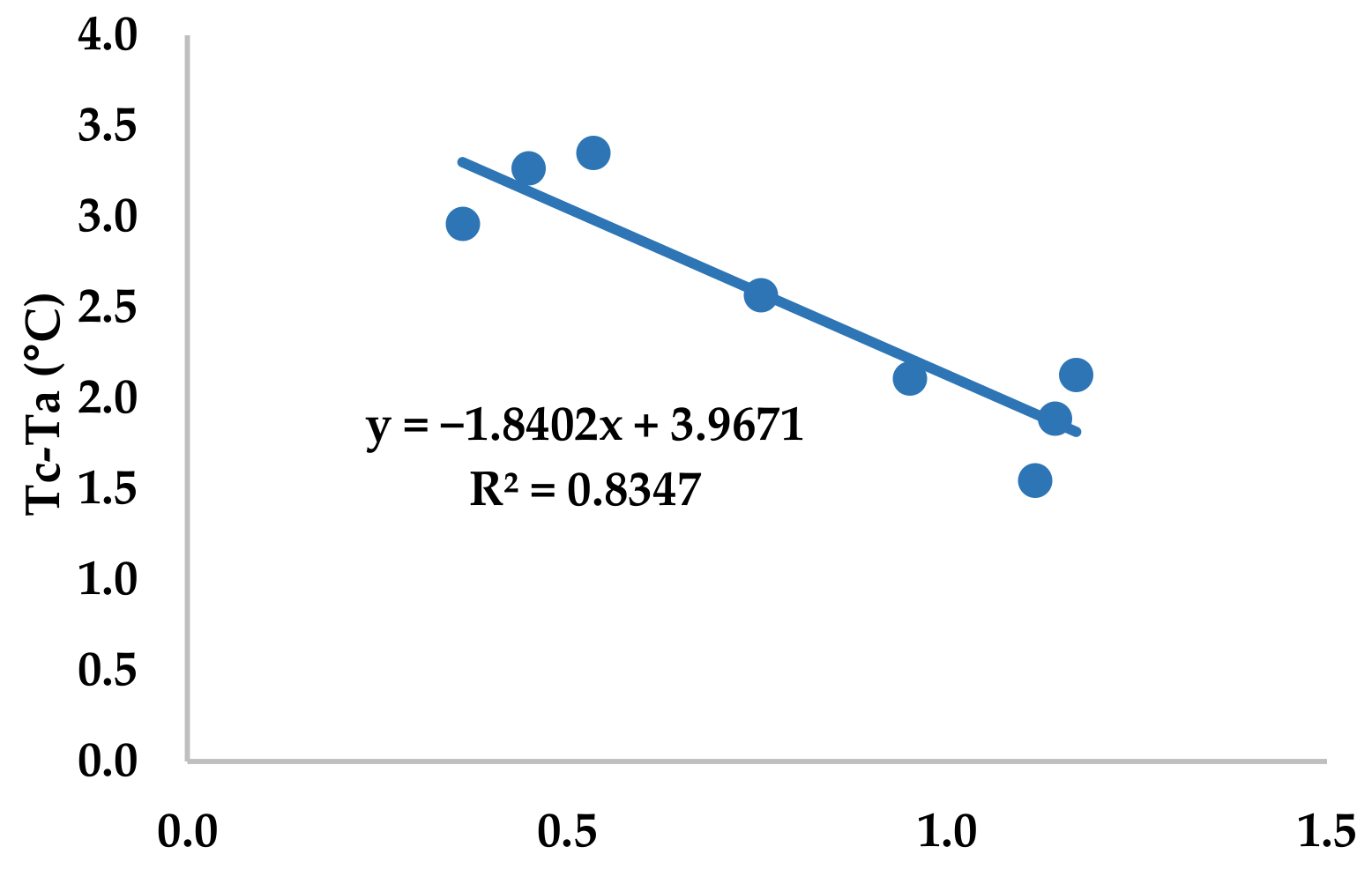
Figure 5 shows the slope and intercept of the NWSB from 2 different days after a rainfall event in the vegetative stage of maize, resulting in the equation shown in the Tc-Ta vs. VPD scatterplot. The same coefficients developed for NWSB were used to determine NTB, using VPG instead of VPD. The relationship between the Tc-Ta and VPD was significant (R2 = 0.84). The Tc − Ta decreased with an increase in VPD.

Figure 5.
Non-water-stressed baselines used to calculate the CWSI for maize at the vegetative growth stage (DOY 93 and 97).
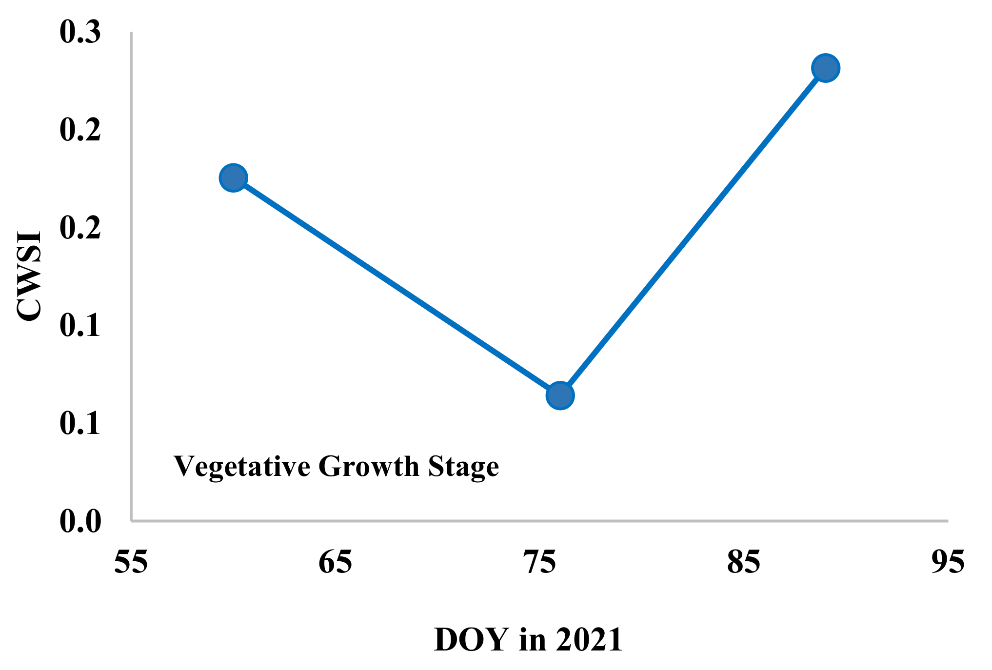
Figure 6 shows the patterns of the CWSI obtained on three different days representing different maize growth stages. Generally, there was low crop water stress, with a peak on DOY 89 (31 March 2021). The lowest CWSI was recorded on DOY 75, showing almost no stress. Maize water stress increases as maize grows and decreases towards the end of the vegetative stage. Figure 5 shows that during the entire stage, maize endured low (<0.5) water stress levels overall.
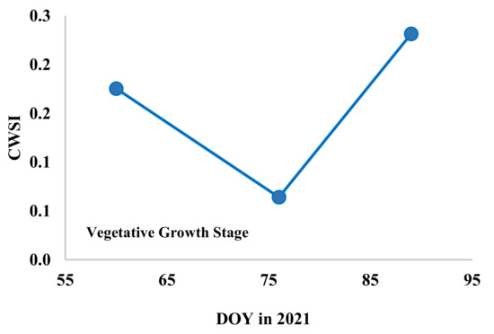
Figure 6.
CWSI for maize in the vegetative stage.
3.2. Exploring the Relationship between the CWSI and Spectral Variables
Table 3 shows the correlation coefficients between the CWSI and the spectral reflectance. The results indicate a link between all the data measured using a UAV and the Crop Water Stress Index. Of the six different bands investigated, the strongest relationship, which was also positive, was observed between the TIR band and the CWSI (r = 0.59). Meanwhile, the other five bands showed a negative relationship with the CWSI. The Red band showed the strongest negative relationship among them all. Similarly, the 21 investigated VIs showed a negative relationship with the CWSI, except for TCARI_OSAVI (r = 0.19) and NDWI (r = 0.35). OSAVI yielded the strongest negative relationship with the CWSI (r = −0.62). All these VIs were derived from the Blue, Green, Red, Red Edge, and NIR bands, which also showed a similar relationship with the CWSI. These findings suggested that the relation between the vegetation indices and the CWSI was slightly higher than that of bands only.

Table 3.
Correlation coefficients r between the CWSI, bands, and VIs.
3.3. Comparing the Performance of Spectral Features in Estimating the Maize Crop Water Stress Index across All Algorithms
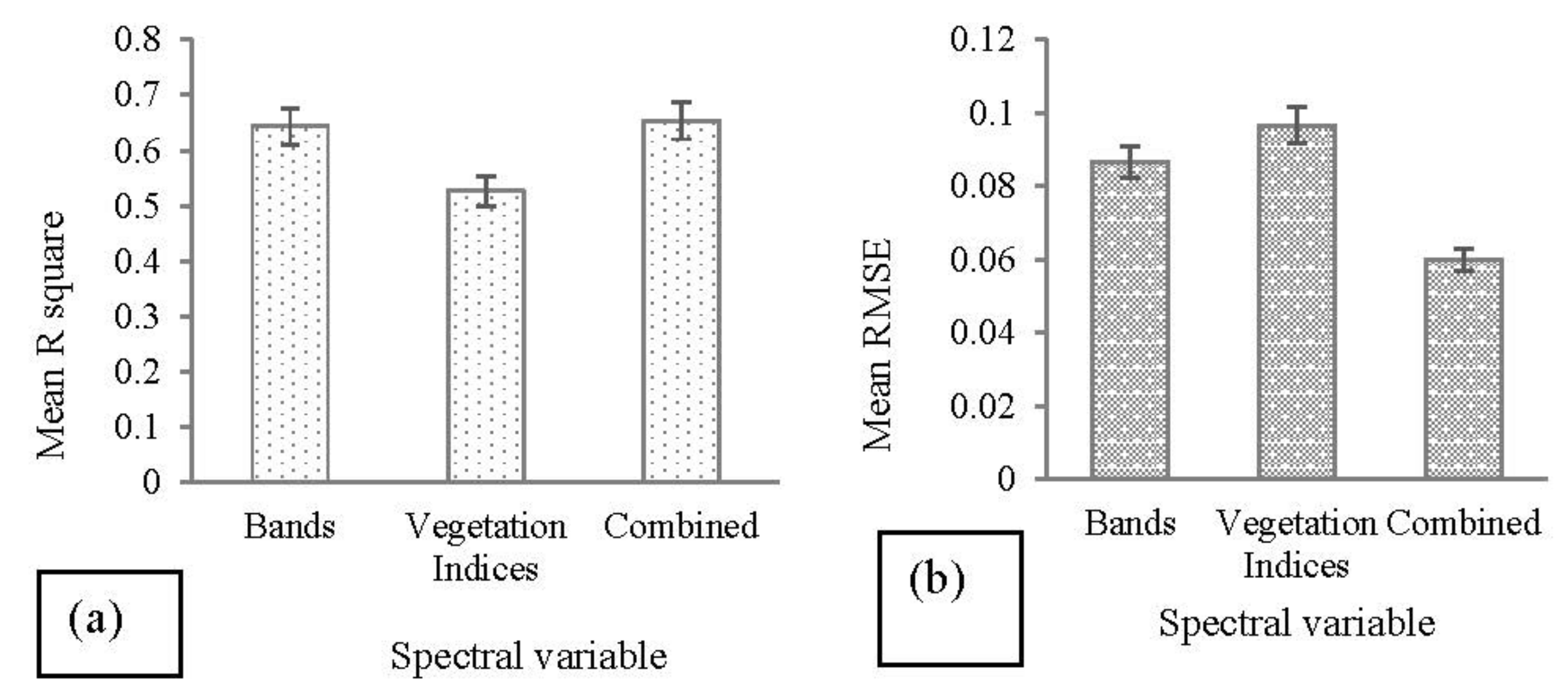
Table 4 shows model accuracies obtained using the PLS, SVM, and RF regression algorithms in predicting the maize CWSI based on the bands, indices, and both datasets combined. The most optimal model, which exhibited a relatively higher R2 (0.85) and lower RMSE (0.05), was derived using a combined dataset of bands and vegetation indices (Figure 7). This was followed by a model derived using bands only, with a RMSE of 0.09. The least accurate model in this study was obtained using vegetation index-only data. Specifically, the vegetation indices yielded an R2 of 0.53 and a RMSE of 0.1. Generally, when the bands were combined with the indices, lower RMSE values were obtained across all models (Table 4).

Table 4.
Prediction accuracies of the CWSI derived using optimal models based on the PLS, SVR, and RF regression models.

Figure 7.
Comparative performance of bands, indices, and combined datasets in predicting the CWSI based on (a) mean R-squares and (b) average RMSEs.
Overall, there was a significant (p = 0.05) difference between the performance of the bands, vegetation indices, and combined datasets (Figure 7). Specifically, the mean RMSE exhibited by the vegetation indices was significantly higher than that exhibited by bands only and the combined datasets. This implied that the vegetation indices did not significantly improve the estimation of the CWSI across all algorithms. Nonetheless, bands only exhibited a relatively lower average RMSE when compared to the vegetation indices. However, their mean RSME was extensively higher than that yielded by the combined datasets (Figure 7). This implied that the combined datasets significantly improved the model accuracies across all algorithms compared to the bands and vegetation indices (Figure 7).
3.4. Comparing the Performance of Machine Learning Algorithms in Estimating Maize Crop Water Stress
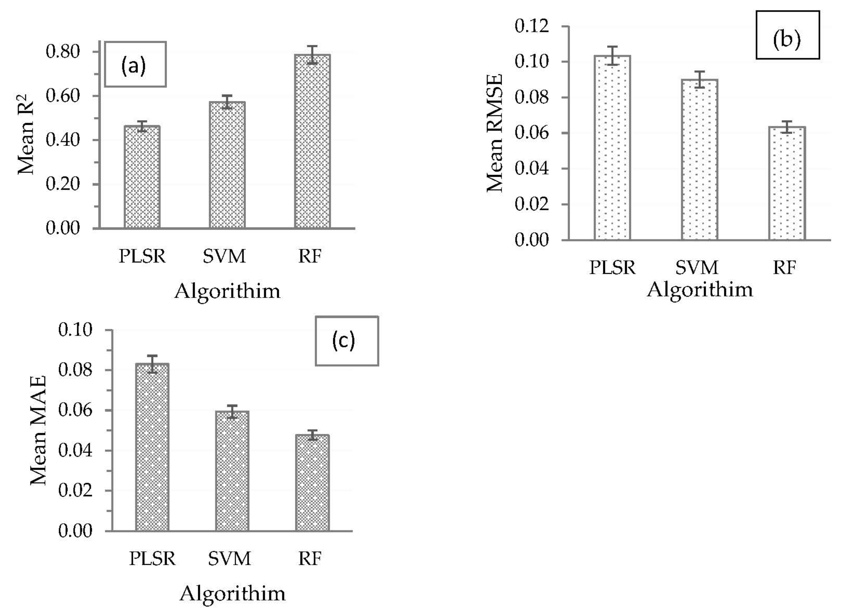
Figure 8 shows the findings from a comparative assessment of the performance of algorithms based on all datasets used in this study. It was observed that RF had the highest mean R2, and the lowest mean RMSE and MAE (R2 = 0.79, RMSE = 0.06, and MAE = 0.05). This implied that RF outperformed SVM and PLSR in estimating the maize CWSI in smallholder croplands. SVM attained the second highest mean R2, and second lowest mean RMSE and mean MAE (R2 = 0.57, RMSE = 0.09, and MAE = 0.06). Meanwhile, PLS had the lowest mean R2, and the highest mean RMSE and MAE (R2 = 0.46, RMSE = 0.1, MAE = 0.08) (Figure 8). Overall, there was a significant difference between the mean RMSE exhibited by PLS, SVM, and RF (Figure 8c). Based on Figure 8, RF emerged as the optimal algorithm for predicting the maize CWSI in smallholder croplands, exhibiting the highest R2, and lowest RMSE and MAE among all models.

Figure 8.
Average (a) R2, (b) RMSE, and (c) MAE derived using the random forest, support vector machine, and partial least squares region algorithms.
3.5. Optimal Models for Estimating the Maize Crop Water Stress Index
The most important variables in the PLS, SVM, and RF models are shown in Figure 9(aii–cii). Ultimately, the PLS model attained an RMSE of 0.1 based on CCCI, MTCI, NDRE, Cl_Red Edge, MTVI2, and other variables (Figure 9a), in that order of importance. Meanwhile, SVM exhibited a RMSE of 0.07 based on TIR, TCAR_SAVI, TCARI_OSAVI, CCCI, and TCARI_RDVI, amongst others, in order of importance. The RF model achieved an RMSE of 0.05 using variables including NDRE, MTCI, CCCI, GNDVI, and TIR in order of importance (Figure 9c).
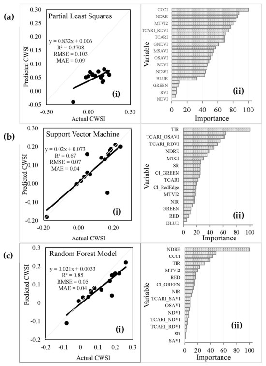
Figure 9.
Relationship between the predicted and observed CWSI derived using combined spectral bands and vegetation indices (i) in conjunction with (a) PLR, (b) SVM, and (c) RF, as well as associated variable importance (ii) models and the model variable importance scores.
3.6. Mapping the Spatial Distribution of Maize Crop Water Stress
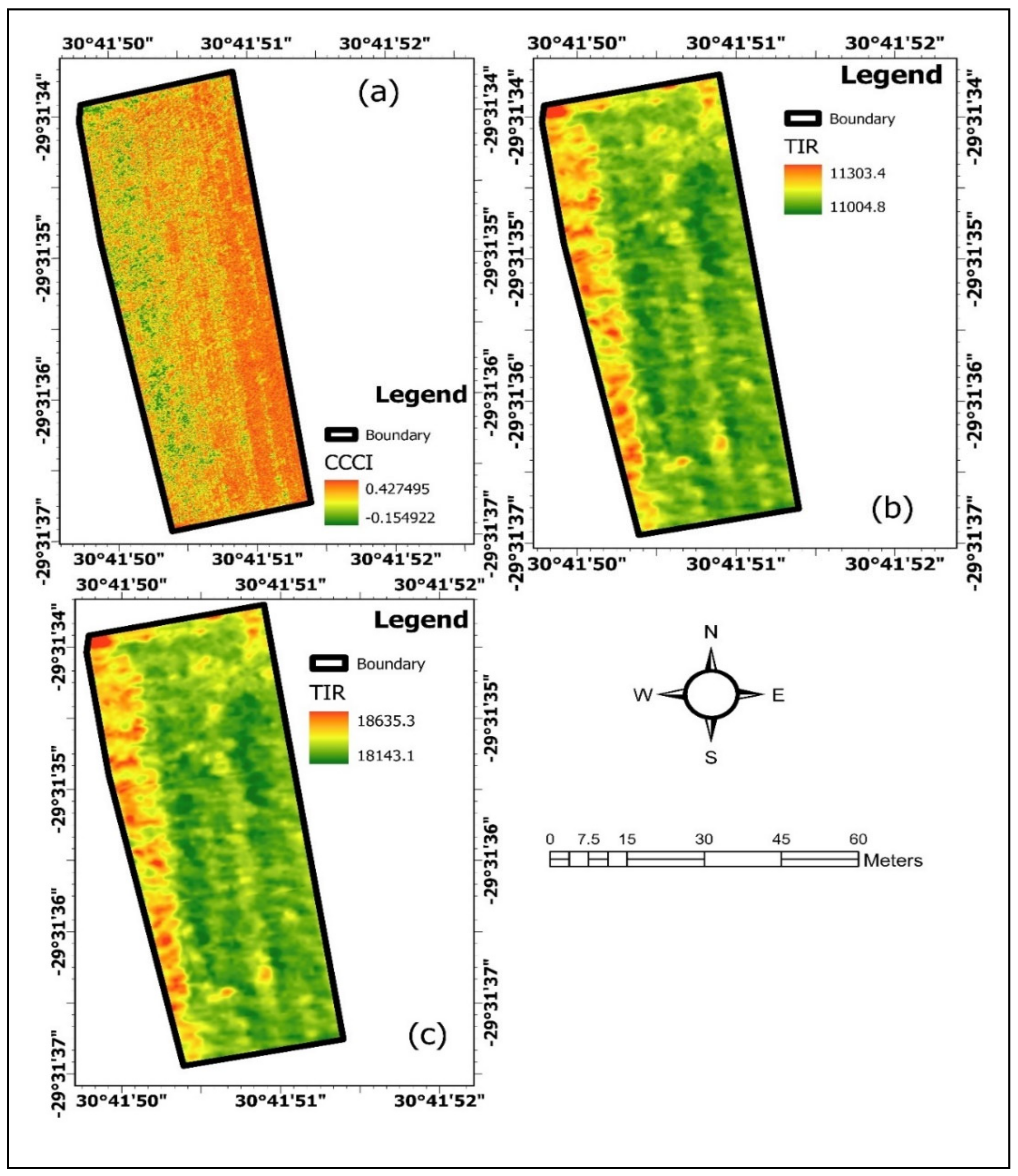
The spatial variation of maize water stress was modelled using the optimal variable in each model. Figure 10 illustrates the spatial variations of maize stress determined using PLS (a), SVM (b), and RF (c). The results indicate that the maize water stress was relatively low throughout the field and increased towards the north and east of the plot (Figure 10b) and west and south of the field (Figure 9c) for the PLS model. On the contrary, the SVM (Figure 9b) modelled map showed an increase eastward towards the edges of the maize plot. The RF-modelled map showed relatively low water stress levels across the field, with no significant spatial variation.

Figure 10.
Spatial distribution of the CWSI developed using the PLS (a), SVM (b), and RF (c) models.
4. Discussion
This study’s objective was to compare PLSR, SVM, and RF performance in estimating the maize CWSI using UAV-acquired remotely sensed data in smallholder croplands typically found in southern Africa. To address this objective, the relative contribution of bands, vegetation indices, and both datasets combined was evaluated.
4.1. Estimating the Crop Water Stress Index
Determining NWSB at each maize growth stage is necessary for determining the CWSI; therefore, NWSB was determined for the vegetative growth stage of maize. The results showed a strong relationship between Tc-Ta and VPD with an R2 of 84. This may be due to the changes in photosynthesis and transpiration during the vegetative stage of maize [15]. Similar relationships were found for maize [31,79]. Furthermore, the results showed that the CWSI was relatively low during this growth stage (CWSI < 0.3). This could be attributed to the rainfall in the area received during this period, which could have replenished the soil with water. According to [82], a significant yield reduction occurs when the CWSI values are greater than 0.40. Moreover, Ref. [83] revealed that the CWSI can detect stress levels 24 to 48 h before the manifestation of visible signs of stress on plants. Therefore, the results of the CWSI could provide a time-efficient insight into the adaptation to climate change and the management of agricultural water resources, which could be a valuable option for smallholder farmers.
4.2. Mapping of the Maize CWSI Using the Optimal Model
The results showed that the maize CWSI was optimally estimated to an RMSE of 0.05 and an MAE of 0.04, based on the spectral reflectance of NDRE, MTCI, CCCI, GNDVI, and TIR as the most significant variables, in order of importance (Figure 9c). The optimal performance of the chlorophyll-based VIs such as NDRE, MTCI, CCCI, and GNDVI could be explained by the fact that the image was acquired during the late vegetative stage characterised by high canopy closure, leaf area index, and chlorophyll content concentrations, indicative of highly photosynthesising maize plants, which indirectly alters the temperature and stomatal conductance of the crop. This explains why chlorophyll-based VIs were influential in this study. The TIR, Red, and Blue bands also demonstrated good performance in the RF model (Figure 9c(ii)). The significance of the TIR to the model could be attributed to the fact that the leaf temperature is primarily determined by the plant’s ability to photosynthesise and the efficiency of the internal leaf structure such as cavities, chloroplasts, and mesophyll cells, compared to ambient temperature [81,82]. Therefore, when a plant is undergoing water stress, molecules in the leaf tissue show signals that induce physiochemical change, which leads to increased foliar temperature concerning air temperature, which explains why it was related to a temperature derived-CWSI in this study [84,85]. In addition, the Blue band has been selected as one of the important variables for estimating CWSI, probably because it is directly related to leaf chlorophyll content. This is attributed to its strong correlation with chlorophyll in green maize crop pigments, driven by absorption for photosynthesis [86]. This also relates to the vegetative growth stage when the maize crop canopy has entirely covered the ground [84], consistent with the low CWSI values obtained.
On the contrary, the NIR band was not very influential in optimally estimating the CWSI. The changes in the leaf structure of maize in the study site were likely not captured well by the MicaSense NIR range camera. As a result, our results do not agree with several other studies which demonstrated that the NIR regions of the electromagnetic spectrum are also influential in detecting and mapping crop water stress at the canopy level [8]. Subsequently, the NDVI was not among the best performing indices. This is aligned with results from other studies, where the NDVI exhibited a low correlation with stomatal conductance [39,40,85]. The high spectral saturation of the NDVI under high vegetation coverage could contribute to this observation. Meanwhile, the impact of the Red Edge band-derived indices could be attributed to their effectiveness in mitigating saturation effects at higher crop foliage density and coverage [86,87,88]. For example, to increase the performance of the RF model, it was found that a combination of traditional vegetative and Red Edge-based indices could be used at the late stage.
4.3. Comparative Performance of Bands, Vegetation Indices, and Combined Datasets
The prediction of CWSI was conducted using three different datasets (bands only, vegetation indices only, and the combination thereof) based on the SVM, RF, and PLSR algorithms. The combined dataset outperformed the bands and VI models in all three modelling scenarios. Specifically, the combined data exhibited a mean RMSE of 0.05 in relation to an RMSE of 0.06 and 0.08 for bands and VIs, respectively. Using the combined data modelling resulted in the most optimal prediction accuracy based on NDRE, MTCI, CCCI, GNDVI, and TIR, as important predictor variables, in order of importance. This indicates that the combination of indices and spectral bands improved the performance of variables that could have saturated under high canopy cover. This could be explained by the fact that combining bands and vegetation indices provides a broader spectral range coverage. Bands capture spectral information in a single section of the electromagnetic spectrum, which is sensitive to a single plant health element or feature, while vegetation indices are derived from combinations of bands from different sections of the electromagnetic spectrum. Subsequently, VIs derive their strength from more than one section of the electromagnetic spectrum, making them sensitive to more features.
Furthermore, VIs tend to reduce the impact of noise on the crop spectral signatures. Therefore, combining bands and VIs ensures sensitivity to various aspects of plant health and physiological conditions such as water stress. Above all, combining these datasets offers a synergistic effect of capturing both structural and physiological aspects of water-stressed crops, enhancing the overall sensitivity and accuracy of the estimation process. Also, health VIs were the most selected estimation features for crop water stress in relation to traditional indices such as the NDVI. The optimal performance of VIs such as NDRE, MTCI, and CCCI could be explained by the ability to circumvent spectral saturation when a crop’s canopy is fully covering the ground. For instance, at high canopy density, the NDVI becomes spectrally saturated [89]. Thus, the results reveal that combining wavelengths with VIs such as NDRE, MTCI, and CCCI improved the estimation accuracies.
However, when VIs only were used, the prediction accuracies were significantly reduced (RMSE = 0.08). This indicates that the traditional indices combined with the chlorophyll-based indices could not detect crop water stress. This is despite the usefulness of indices such as TCARI in reducing non-photosynthetic background noise [89]. Generally, VIs improve estimation accuracies, as water stress accumulates [31]. However, this study was conducted during the vegetative stage when water stress was limited due to the frequent precipitation in the study area.
Contrary to the findings of this study, Refs. [31,39] demonstrated a strong correlation between VIs and water stress indicators during the late reproductive and maturation stages of the crops. Similarly, Ref. [39] found that the TCARI/OSAVI improved from R2 of 0.58 to 0.84 during the late vegetative and maturation stages, respectively. Their results demonstrated that as water stress accumulates, VIs become more sensitive. Our results are supported by those of [25], which also demonstrated relatively low-performance VI-only data in predicting the maize CWSI.
Meanwhile, bands only demonstrated a significant relationship with the maize CWSI. In particular, the TIR band was the most optimal in the RF model. This could be attributed to the fact that there was full vegetation cover, and the lack of soil background disturbance allowed the measurement of canopy temperature and stomatal conductance resulting from water utilisation [55,89]. This shows that the bands were able to capture the changes in canopy temperature. This is supported by the literature where water stress in agricultural plants was detected using remote canopy temperature measurements on a TIR basis [12,90].
4.4. The Performance of Machine Learning Algorithms in Predicting the Maize Crop Water Stress Index (CWSI)
The findings of this study demonstrated that RF optimally outperformed SVM and PLSR at single analysis stages (Table 4) and across all stages when findings were pooled (Figure 7). Specifically, RF optimally predicted the CWSI to an RMSE of 0.05, an MAE of 0.04, and an R2 equivalent to 0.85 across all datasets. The optimal performance of RF could be attributed to its ease of optimisation and execution compared to other algorithms. Additionally, RF can tolerate highly correlated variables, such as bands combined with vegetation indices [49,91,92,93,94]. RF, being a non-linear method, offers high simulation accuracy and a very flexible model-building process, making it robust in comparison to other algorithms [95].
Furthermore, the RF excels in modelling non-linear dimensional relationships while preventing overfitting. Importantly, RF demonstrates relative robustness regarding noise detection in data, the establishment of an impartial estimate of error rate, and the capacity to determine the relevance of optimal predictor variables for modelling [78,89]. Similarly, the algorithm has been proven optimal in predicting crop water stress for crops such as rice [96] and wheat [97]. Consistent with these studies, RF outperformed SVM and PLS.
SVM produced the second best results in the prediction of the CWSI (RMSE = 0.067, MAE = 0.07). Its strength lies in handling outliers, showcasing substantial generalization capability when dealing with unseen patterns [98]. This model is reliable for the regression of small linear and high-dimensional samples [99], which may explain its superior performance compared to PLS. Another advantage of SVM is its effective processing of data acquired with few samples, as demonstrated in this study, without compromising resultant accuracies [98]. In contrast, PLS performed least well in effectively estimating the CWSI across all dataset scenarios (RMSE = 0.086, MAE = 0.073).
PLS cannot handle data conditions such as high dimensionality and the correlation of predictor variables, which may explain its poor performance [91]. In addition, due to PLS’s tendency to struggle with collinear variables, as observed in this study, non-linear relationships between predictor variables and certain crop parameters could have contributed to poor performance [99]. Moreover, the literature notes that PLS is best suited for large training datasets [100]. Future considerations may involve exploring a larger sample size to enhance the accuracy of PLS prediction for maize crop water stress in smallholder farms. Furthermore, exploring other machine learning algorithms could be beneficial in finding an optimal model to substitute PLS.
5. Conclusions
This study sought to assess the performance of PLSR, SVM, and RF in estimating the maize CWSI using UAV-acquired remotely sensed data in smallholder croplands typically found in southern Africa. To address this objective, the relative contribution of bands, vegetation indices, and both datasets combined was evaluated. Grounded on the results of this study, the following conclusions can be drawn:
- RF proved to be the most suitable algorithm for predicting the maize CWSI in smallholder croplands, utilising NDRE, MTCI, CCCI, GNDVI, and TIR, as important predictor variables, listed in order of importance. Specifically, RF was optimal compared to PLS and SVM, resulting in the highest R2 (0.79) and the lowest MAE (0.06) and RMSE (0.05) on average in three different data groups (bands only, VI only, and combined data).
- Combining bands and vegetation indices resulted in the best prediction of the maize CWSI compared to using these variables separately. Specifically, the two models, SVM and RF, improved when the analysis was performed with the combined data compared to when performed with bands only or indices only, resulting in the lowest RMSE of 0.07 and 0.05 for SVM and RF, respectively.
In conclusion, these results demonstrate that the UAV data could be used optimally to forecast the water stress of maize crops on a smaller scale. These results indicate that the UAV multispectral camera could capture the spatial variation of maize crop water stress at a field scale. This further concurs with the notion that adopting cutting-edge technologies, e.g., machine learning, remote sensing, and UAVs, plays a crucial role in the future of smallholder agricultural systems. The findings from this study indicate that using UAV technologies in smallholder farms in conjunction with machine learning algorithms such as the RF model holds promise for improving the management of agricultural crops for improved production. Moreover, UAV technology provides near-real-time information beneficial to farmers for early preparedness and response to improve crop productivity. These findings contribute to precision agriculture, involving advanced technologies and analytical methods for the near-real-time monitoring and mapping of crop water stress in staple crops such as maize. This is particularly relevant in developing regions where food and nutrition insecurity have been reported. The implications extend to sustainable agriculture and food security in regions facing water-related issues.
Author Contributions
Conceptualization, M.K. and M.S.; methodology, M.K. and M.S.; formal analysis, M.K.; writing—original draft preparation, M.K. and M.S.; writing—review and editing, M.S., J.M., T.M., L.N. and S.M.; supervision, M.S., J.M. and T.M.; funding acquisition, T.M. All authors have read and agreed to the published version of the manuscript.
Funding
This research was funded by Water Research Commission under Project K5/2971//4.
Data Availability Statement
Data will be provided upon request. To request the data, please contact Mbulisi Sibanda msibanda@uwc.ac.za.
Conflicts of Interest
The authors declare that they have no conflict of interest to disclose concerning their manuscript.
References
- Simanjuntak, C.; Gaiser, T.; Ahrends, H.E.; Ceglar, A.; Singh, M.; Ewert, F.; Srivastava, A. Impact of climate extreme events and their causality on maize yield in South Africa. Sci. Rep. 2023, 13, 12462. [Google Scholar] [CrossRef] [PubMed]
- Grote, U.; Fasse, A.; Nguyen, T.; Erenstein, O. Food security and the dy-namics of wheat and maize value chains in Africa and Asia. Front. Sustain. Food Syst. 2021, 4, 617009. [Google Scholar] [CrossRef]
- Gerhards, M.; Schlerf, M.; Rascher, U.; Udelhoven, T.; Juszczak, R.; Alberti, G.; Miglietta, F.; Inoue, Y. Analysis of airborne optical and thermal imagery for detection of water stress symptoms. Remote Sens. 2018, 10, 1139. [Google Scholar] [CrossRef]
- Bradshaw, C.D.; Pope, E.; Kay, G.; Davie, J.C.; Cottrell, A.; Bacon, J.; Cosse, A.; Dunstone, N.; Jennings, S.; Challinor, A.; et al. Unprecedented climate extremes in South Africa and implications for maize production. Environ. Res. Lett. 2022, 17, 084028. [Google Scholar] [CrossRef]
- Ferreira, N.C.R.; Rötter, R.P.; Bracho-Mujica, G.; Nelson, W.C.D.; Lam, Q.D.; Recktenwald, C.; Abdulai, I.; Odhiambo, J.; Foord, S. Drought patterns: Their spatiotemporal variability and impacts on maize production in Limpopo province, South Africa. Int. J. Biometeorol. 2023, 67, 133–148. [Google Scholar] [CrossRef]
- Pradawet, C.; Khongdee, N.; Pansak, W.; Spreer, W.; Hilger, T.; Cadisch, G. Thermal imaging for assessment of maize water stress and yield prediction under drought conditions. J. Agron. Crop Sci. 2023, 209, 56–70. [Google Scholar] [CrossRef]
- Ahmad, U.; Alvino, A.; Marino, S. A review of crop water stress assessment using remote sensing. Remote Sens. 2021, 13, 4155. [Google Scholar] [CrossRef]
- Berni, J.A.J.; Zarco-Tejada, P.J.; Sepulcre-Cantó, G.; Fereres, E.; Villalobos, F. Mapping canopy conductance and CWSI in olive orchards using high resolution thermal remote sensing imagery. Remote Sens. Environ. 2009, 113, 2380–2388. [Google Scholar] [CrossRef]
- Buckley, T.N. How do stomata respond to water status? New Phytol. 2019, 224, 21–36. [Google Scholar] [CrossRef] [PubMed]
- Kögler, F.; Söffker, D. Explorative frequency analysis of leaf temperature behavior of maize (Zea mays subsp. mays) at water deficit. Plants 2019, 8, 105. [Google Scholar] [CrossRef] [PubMed]
- Ramírez-Cuesta, J.M.; Ortuño, M.F.; Gonzalez-Dugo, V.; Zarco-Tejada, P.J.; Parra, M.; Rubio-Asensio, J.S.; Intrigliolo, D.S. Assessment of peach trees water status and leaf gas exchange using on-the-ground versus airborne-based thermal imagery. Agric. Water Manag. 2022, 267, 107628. [Google Scholar] [CrossRef]
- Idso, S.B.; Jackson, R.D.; Pinter, P.J.; Reginato, R.J.; Hatfield, J.L. Normalizing the stress-degree-day parameter for environmental variability. Agric. Meteorol. 1981, 24, 45–55. [Google Scholar] [CrossRef]
- Jackson, R.D.; Idso, S.B.; Reginato, R.J.; Pinter, P.J. Canopy temperature as a crop water stress indicator. Water Resour. Res. 1981, 17, 1133–1138. [Google Scholar] [CrossRef]
- Poblete-Echeverría, C.; Espinace, D.; Sepúlveda-Reyes, D.; Zuniga, M.; Sanchez, M. Analysis of crop water stress index (CWSI) for estimating stem water potential in grapevines: Comparison between natural reference and baseline approaches. Acta Hortic. 2018. [Google Scholar] [CrossRef]
- Ru, C.; Hu, X.; Wang, W.; Ran, H.; Song, T.; Guo, Y. Evaluation of the Crop Water Stress Index as an Indicator for the Diagnosis of Grapevine Water Deficiency in Greenhouses. Horticulturae 2020, 6, 86. [Google Scholar] [CrossRef]
- Egea, G.; Padilla-Díaz, C.M.; Martinez-Guanter, J.; Fernández, J.E.; Pérez-Ruiz, M. Assessing a crop water stress index derived from aerial thermal imaging and infrared thermometry in super-high density olive orchards. Agric. Water Manag. 2017, 187, 210–221. [Google Scholar] [CrossRef]
- Park, S.; Ryu, D.; Fuentes, S.; Chung, H.; O’connell, M.; Kim, J. Dependence of cwsi-based plant water stress estimation with diurnal acquisition times in a nectarine orchard. Remote Sens. 2021, 13, 2775. [Google Scholar] [CrossRef]
- Gonzalez-Dugo, V.; Zarco-Tejada, P.J.; Intrigliolo, D.S.; Ramírez-Cuesta, J.M. Normalization of the crop water stress index to assess the within-field spatial variability of water stress sensitivity. Precis. Agric. 2021, 22, 964–983. [Google Scholar] [CrossRef]
- Rud, R.; Cohen, Y.; Alchanatis, V.; Levi, A.; Brikman, R.; Shenderey, C.; Heuer, B.; Markovitch, T.; Dar, Z.; Rosen, C.; et al. Crop water stress index derived from multi-year ground and aerial thermal images as an indicator of potato water status. Precis. Agric. 2014, 15, 273–289. [Google Scholar] [CrossRef]
- Ekinzog, E.K.; Schlerf, M.; Kraft, M.; Werner, F.; Riedel, A.; Rock, G.; Mallick, K. Revisiting crop water stress index based on potato field experiments in Northern Germany. Agric. Water Manag. 2022, 269, 107664. [Google Scholar] [CrossRef]
- Nouraki, A.; Akhavan, S.; Rezaei, Y.; Fuentes, S. Assessment of sunflower water stress using infrared thermometry and computer vision analysis. Water Sci. Technol. Water Supply 2021, 21, 1228–1242. [Google Scholar] [CrossRef]
- Orta, A.H.; Erdem, T.; Erdem, Y. Determination of water stress index in sunflower. Helia 2002, 25, 27–38. [Google Scholar] [CrossRef][Green Version]
- Mwinuka, P.R.; Mbilinyi, B.P.; Mbungu, W.B.; Mourice, S.K.; Mahoo, H.F.; Schmitter, P. The feasibility of hand-held thermal and UAV-based multispectral imaging for canopy water status assessment and yield prediction of irrigated African eggplant (Solanum aethopicum L). Agric. Water Manag. 2021, 245, 106584. [Google Scholar] [CrossRef]
- Qin, A.; Ning, D.; Liu, Z.; Li, S.; Zhao, B.; Duan, A. Determining threshold values for a crop water stress index-based center pivot irrigation with optimum grain yield. Agriculture 2021, 11, 958. [Google Scholar] [CrossRef]
- Zhang, T.X.; Su, J.Y.; Liu, C.J.; Chen, W.H. Potential Bands of Sentinel-2A Satellite for Classification Problems in Precision Agriculture. Int. J. Autom. Comput. 2019, 16, 16–26. [Google Scholar] [CrossRef]
- Gu, S.J.; Liao, Q.; Gao, S.Y.; Kang, S.Z.; Du, T.S.; Ding, R.S. Crop Water Stress Index as a Proxy of Phenotyping Maize Performance under Combined Water and Salt Stress. Remote Sens. 2021, 13, 4710. [Google Scholar] [CrossRef]
- Carroll, D.A.; Hansen, N.C.; Hopkins, B.G.; DeJonge, K.C. Leaf temperature of maize and Crop Water Stress Index with variable irrigation and nitrogen supply. Irrig. Sci. 2017, 35, 549–560. [Google Scholar] [CrossRef]
- Zhang, L.; Zhang, H.; Zhu, Q.; Niu, Y. Further investigating the performance of crop water stress index for maize from baseline fluctuation, effects of environmental factors, and variation of critical value. Agric. Water Manag. 2023, 285, 108349. [Google Scholar] [CrossRef]
- Pipatsitee, P.; Tisarum, R.; Taota, K.; Samphumphuang, T.; Eiumnoh, A.; Singh, H.P.; Cha-um, S. Effectiveness of vegetation indices and UAV-multispectral imageries in assessing the response of hybrid maize (Zea mays L.) to water deficit stress under field environment. Environ. Monit. Assess. 2023, 195, 128. [Google Scholar] [CrossRef] [PubMed]
- Tandzi, L.N.; Mutengwa, C.S. Estimation of Maize (Zea mays L.) Yield Per Harvest Area: Appropriate methods. Agronomy 2020, 10, 29. [Google Scholar] [CrossRef]
- Zhang, F.; Zhou, G. Estimation of vegetation water content using hyperspectral vegetation indices: A comparison of crop water indicators in response to water stress treatments for summer maize. BMC Ecol. 2019, 19, 18. [Google Scholar] [CrossRef]
- Jin, N.; He, J.Q.; Fang, Q.X.; Chen, C.; Ren, Q.F.; He, L.; Yao, N.; Song, L.B.; Yu, Q. The Responses of Maize Yield and Water Use to Growth Stage-Based Irrigation on the Loess Plateau in China. Int. J. Plant Prod. 2020, 14, 621–633. [Google Scholar] [CrossRef]
- Mulla, D.J. Twenty five years of remote sensing in precision agriculture: Key advances and remaining knowledge gaps. Biosyst. Eng. 2013, 4, 358–371. [Google Scholar] [CrossRef]
- Bian, J.; Zhang, Z.; Chen, J.; Chen, H.; Cui, C.; Li, X.; Chen, S.; Fu, Q. Simplified evaluation of cotton water stress using high resolution unmanned aerial vehicle thermal imagery. Remote Sens. 2019, 11, 267. [Google Scholar] [CrossRef]
- Zhang, L.; Niu, Y.; Zhang, H.; Han, W.; Li, G.; Tang, J.; Peng, X. Maize Canopy Temperature Extracted From UAV Thermal and RGB Imagery and Its Application in Water Stress Monitoring. Front. Plant Sci. 2019, 10, 1270. [Google Scholar] [CrossRef]
- Aldubai, A.A.; Alsadon, A.A.; Al-Gaadi, K.A.; Tola, E.K.; Ibrahim, A.A. Utilizing spectral vegetation indices for yield assessment of tomato genotypes grown in arid conditions. Saudi J. Biol. Sci. 2022, 29, 2506–2513. [Google Scholar] [CrossRef]
- Lee, H.; Wang, J.; Leblon, B. Using linear regression, random forests, and support vector machine with unmanned aerial vehicle multispectral images to predict canopy nitrogen weight in corn. Remote Sens. 2020, 12, 2071. [Google Scholar] [CrossRef]
- Giovos, R.; Tassopoulos, D.; Kalivas, D.; Lougkos, N.; Priovolou, A. Remote sensing vegetation indices in viticulture: A critical review. Agriculture 2021, 11, 457. [Google Scholar] [CrossRef]
- Baluja, J.; Diago, M.P.; Balda, P.; Zorer, R.; Meggio, F.; Morales, F.; Tardaguila, J. Assessment of vineyard water status variability by thermal and multispectral imagery using an unmanned aerial vehicle (UAV). Irrig. Sci. 2012, 30, 511–522. [Google Scholar] [CrossRef]
- Gago, J.; Douthe, C.; Coopman, R.E.; Gallego, P.P.; Ribas-Carbo, M.; Flexas, J.; Escalona, J.; Medrano, H. Uavs challenge to assess water stress for sustainable agriculture. Agric. Water Manag. 2015, 153, 9–19. [Google Scholar] [CrossRef]
- Espinoza, C.Z.; Khot, L.R.; Sankaran, S.; Jacoby, P.W. High Resolution Multispectral and Thermal Remote Sensing-Based Water Stress Assessment in Subsurface Irrigated Grapevines. Remote Sens. 2017, 9, 961. [Google Scholar] [CrossRef]
- Zarco-Tejada, P.J.; Gonzalez-Dugo, V.; Williams, L.E.; Suarez, L.; Berni, J.A.J.; Goldhamer, D.; Fereres, E. A PRI-based water stress index combining structural and chlorophyll effects: Assessment using diurnal narrow-band airborne imagery and the CWSI thermal index. Remote Sens. Environ. 2013, 138, 38–50. [Google Scholar] [CrossRef]
- Raczko, E.; Zagajewski, B. Comparison of support vector machine, random forest and neural network classifiers for tree species classification on airborne hyperspectral APEX images. Eur. J. Remote Sens. 2017, 50, 144–154. [Google Scholar] [CrossRef]
- Cai, J.; Lou, J.; Wang, S.; Yang, S. Feature selection in machine learning: A new perspective. Neurocomputing 2018, 300, 70–79. [Google Scholar] [CrossRef]
- Mochida, K.; Koda, S.; Inoue, K.; Hirayama, T.; Tanaka, S.; Nishii, R.; Melgani, F. Computer vision-based phenotyping for improvement of plant productivity: A machine learning perspective. Gigascience 2019, 8, giy153. [Google Scholar] [CrossRef] [PubMed]
- Singhal, G.; Bansod, B.; Mathew, L.; Goswami, J.; Choudhury, B.U.; Raju, P.L.N. Chlorophyll estimation using multi-spectral unmanned aerial system based on machine learning techniques. Remote Sens. Appl. Soc. Environ. 2019, 15, 100235. [Google Scholar] [CrossRef]
- Alabi, T.R.; Abebe, A.T.; Chigeza, G.; Fowobaje, K.R. Estimation of soybean grain yield from multispectral high-resolution UAV data with machine learning models in West Africa. Remote Sens. Appl. Soc. Environ. 2022, 27, 100782. [Google Scholar] [CrossRef]
- Ndlovu, H.S.; Odindi, J.; Sibanda, M.; Mutanga, O.; Clulow, A.; Chimonyo, V.G.P.; Mabhaudhi, T. A comparative estimation of maize leaf water content using machine learning techniques and unmanned aerial vehicle (Uav)-based proximal and remotely sensed data. Remote Sens. 2021, 13, 4091. [Google Scholar] [CrossRef]
- Ma, D.; Rehman, T.U.; Zhang, L.; Maki, H.; Tuinstra, M.R.; Jin, J. Modeling of diurnal changing patterns in airborne crop remote sensing images. Remote Sens. 2021, 13, 1719. [Google Scholar] [CrossRef]
- Guo, Y.; Yin, G.; Sun, H.; Wang, H.; Chen, S.; Senthilnath, J.; Wang, J.; Fu, Y. Scaling effects on chlorophyll content estimations with RGB camera mounted on a UAV platform using machine-learning methods. Sensors 2020, 20, 5130. [Google Scholar] [CrossRef]
- Yang, M.; Gao, P.; Chen, W.; Zhou, P.; Sun, D.; Xie, J.; Lu, J.; Wang, W. Research of Brassica chinensis var. parachinensis under water stress based on machine learning. J. South China Agric. Univ. 2021, 42, 117–126. [Google Scholar] [CrossRef]
- Adam, E.M.I.; Ismail, R.; Mutanga, O. A comparison of selected machine learning classifiers in mapping a South African heterogeneous coastal zone: Testing the utility of an object-based classification with WorldView-2 imagery. Int. J. Remote Sens. 2012, 8538, 177–186. [Google Scholar]
- Masenyama, A.; Mutanga, O.; Dube, T.; Sibanda, M.; Odebiri, O.; Mabhaudhi, T. Inter-Seasonal Estimation of Grass Water Content Indicators Using Multisource Remotely Sensed Data Metrics and the Cloud-Computing Google Earth Engine Platform. Appl. Sci. 2023, 13, 3117. [Google Scholar] [CrossRef]
- Brewer, K.; Clulow, A.D.; Sibanda, M.; Gokool, S.; Naiken, V.; Mabhaudhi, T.T. Predicting the chlorophyll content of maize over phrnotyping as aproxy for crop health in smallholder farming systems. Remote Sens. 2022, 3, 518. [Google Scholar] [CrossRef]
- Costa, C.; Dwyer, L.; Dutilleul, P.; Stewart, D.; Ma, B.; Smith, D. Sample size determination for chlorophyll meter readings on maize hybrids with a broad range of canopy types. J. Plant Nutr. 2003, 8, 1173–1194. [Google Scholar] [CrossRef]
- Allen, R.G.; Pereira, L.S.; Raes, D.; Smith, M. FAO Irrigation and Drainage Paper No. 56—Crop Evapotranspiration; Food and Agriculture Organisation of the United Nations: Rome, Italy, 1998. [Google Scholar]
- Taghvaeian, S.; Chávez, J.L.; Hansen, N.C. Infrared thermometry to estimate crop water stress index and water use of irrigated maize in northeastern colorado. Remote Sens. 2012, 4, 3619–3637. [Google Scholar] [CrossRef]
- Yue, J.; Feng, H.; Yang, G.; Li, Z. A comparison of regression techniques for estimation of above-ground winter wheat biomass using near-surface spectroscopy. Remote Sens. 2018, 10, 66. [Google Scholar] [CrossRef]
- Rouse, J.W.; Haas, R.H.; Schell, J.A.; Deering, D.W. Monitoring vegetation systems in the Great Plains with ERTS. NASA Spec. Publ. 1974, 1, 309. [Google Scholar]
- Gileston, A.; Kaufman, Y.; Merzlyak, M. Use of a green channel in remote sensing of global vegetation from EOS-MODIS. Remote Sens. Envron. 1996, 3, 289–298. [Google Scholar]
- Fitzgerald, G.; Rodriguez, D.; O’leary, G. Measuring and predicting canopy nitrogen nutrition in wheat using a spectral index—The canopy chlorophyll content index (CCCI). Field crops Res. 2010, 3, 318–324. [Google Scholar] [CrossRef]
- Xue, J.; Su, B. Significant remote sensing vegetation indices: A review of developments and applications. J. Sens. 2017, 1, 1–17. [Google Scholar] [CrossRef]
- Zhang, F.; Zhou, G. Estimation of canopy water content by means of hyperspectral indices based on drought stress gradient experiments of maize in the north plain China. Remote Sens. 2015, 7, 15203–15223. [Google Scholar] [CrossRef]
- Gitelson, A.; Merzlyak, M. Quantitative estimation of chlorophyll-a using reflectance spectra: Experiments with autumn chestnut and maple leaves. J. Photochem. Photobiol. B Biol. 1994, 3, 247–252. [Google Scholar] [CrossRef]
- Bannari, A.; Morin, D.; Bonn, F.; Huete, A.R. A review of vegetation indices. Remote Sens. Rev. 1995, 13, 95–120. [Google Scholar] [CrossRef]
- Baret, F.; Guyot, G. Potentials and limits of vegetation indices for LAI and APAR assessment. Remote Sens. Environ. 1991, 35, 161–173. [Google Scholar] [CrossRef]
- Liu, J.; Pattey, E.; Miller, J.R.; McNairn, H.; Smith, A.; Hu, B. Estimating crop stresses, aboveground dry biomass and yield of corn using multi-temporal optical data combined with a radiation use efficiency model. Remote Sens. Environ. 2010, 114, 1167–1177. [Google Scholar] [CrossRef]
- Varco, J.J.; Fox, A.A.; Raper, T.B.; Hubbard, K.J. Development of sensor based detection of crop nitrogen status for utilization in variable rate nitrogen fertilization. In Precision Agriculture’13; Wageningen Academic Publishers: Wageningen, The Netherlands, 2013. [Google Scholar]
- Dash, J.; Curran, P.J. The MERIS terrestrial chlorophyll index. Int. J. Remote Sens. 2004, 25, 5403–5413. [Google Scholar] [CrossRef]
- Özelkan, E. Water body detection analysis using NDWI indices derived from landsat-8 OLI. Polish J. Environ. Stud. 2020, 29, 1759–1769. [Google Scholar] [CrossRef] [PubMed]
- Jordan, C.F. Derivation of Leaf-Area Index from Quality of Light on the Forest Floor. Ecology 1969, 50, 663–666. [Google Scholar] [CrossRef]
- Haboudane, D.; Miller, J.R.; Pattey, E.; Zarco-Tejada, P.J.; Strachan, I.B. Hyperspectral vegetation indices and novel algorithms for predicting green LAI of crop canopies: Modeling and validation in the context of precision agriculture. Remote Sens. Environ. 2004, 3, 337–352. [Google Scholar] [CrossRef]
- Haaland, D.M.; Thomas, E. Partial least-squares methods for spectral analyses. 1. Relation to other quantitative calibration methods and the extraction of qualitative information. Anal. Chem. 1988, 60, 1193–1202. [Google Scholar] [CrossRef]
- Geladi, P.; Kowalshi, B.R. Partial least-squares regression: A tutorial. Anal. Chim. Acta 1986, 185, 1–17. [Google Scholar] [CrossRef]
- Martens, H.; Naes, T. Multivariate Calibration; John Wiley & Sons: Hoboken, NJ, USA, 1992. [Google Scholar]
- Wold, S.; Sjostrom, M.; Eriksson, L. Pls_regression: A basic tool of chemomrics. Chemom. Intell. Lab. Syst. 2001, 58, 109–130. [Google Scholar] [CrossRef]
- Krishna, G.; Sahoo, R.N.; Singh, P.; Bajpai, V.; Patra, H.; Kumar, S.; Dandapani, R.; Gupta, V.K.; Viswanathan, C.; Ahmad, T.; et al. Comparison of various modelling approaches for water deficit stress monitoring in rice crop through hyperspectral remote sensing. Agric. Water Manag. 2019, 213, 231–244. [Google Scholar] [CrossRef]
- Kuhn, M.; Johnson, K. Applied Predictive Modeling; Springer: New York, NY, USA, 2013; ISBN 9781461468493. [Google Scholar]
- Mashiane, K.; Adelabu, S.; Ramoelo, A. Comperative Analysis of Single Bands, Vegetation Indices, and Their Combination in Predicting Grass Species Nitrogen in a Protected Mountainous Area. Appl. Sci. 2023, 13, 7960. [Google Scholar] [CrossRef]
- Eugenio, F.C.; Grohs, M.; Venancio, L.P.; Schuh, M.; Bottega, E.L.; Ruoso, R.; Schons, C.; Mallmann, C.L.; Badin, T.L.; Fernandes, P. Estimation of soybean yield from machine learning techniques and multispectral RPAS imagery. Remote Sens. Appl. Soc. Environ. 2020, 20, 100397. [Google Scholar] [CrossRef]
- Nguyen, Q.H.; Ly, H.B.; Ho, L.S.; Al-Ansari, N.; Van Le, H.; Tran, V.Q.; Prakash, I.; Pham, B.T. Influence of data splitting on performance of machine learning models in prediction of shear strength of soil. Math. Probl. Eng. 2021, 2021, 4832864. [Google Scholar] [CrossRef]
- Jamshidi, S.; Zand-Parsa, S.; Kamgar-Haghighi, A.A.; Shahsavar, A.R.; Niyogi, D. Evapotranspiration, Crop Coefficients, and Physiological Responses of Citrus Trees in Semi-arid Climatic Conditions. Agric. Water Manag. 2020, 227, 105838. [Google Scholar] [CrossRef]
- Kacira, M.; Ling, P.P.; Short, T.H. Establishing Crop Water Stress Index (CWSI) Threshold Values for Early, Non–contact Detection of Plant Water Stress. Trans. ASAE 2002, 3, 775. [Google Scholar] [CrossRef]
- Zhang, Y.; Xiaowei, D.; Chen, Z.; Hou, G. A study on the physiological parameters of corn during the jointing stage of growth under soil water stress based on the PSII light quantum yield (QY). HydroResearch 2023, 6, 177–183. [Google Scholar] [CrossRef]
- Zhang, L.; Yan, M.; Ren, Y.; Chen, Y.; Zhang, S. Zinc regulates the hydraulic response of maize root under water stress conditions. Plant Physiol. Biochem. 2021, 159, 123–134. [Google Scholar] [CrossRef]
- Cai, F.; Zhang, Y.; Mi, N.; Ming, H.; Zhang, S.; Zhang, H.; Zhao, X. Maize (Zea mays L.) physiological responses to drought and rewatering, and the associations with water stress degree. Agric. Water Manag. 2020, 241, 106379. [Google Scholar] [CrossRef]
- Ustin, S.; Jacqueemoud, S. How the optical properties of leaves modify the absorption and scattering of energy and enhance leaf functionality. Remote Sens. Plant Biodivers. 2020, 349–384. [Google Scholar]
- Zhu, W.; Sun, Z.; Yang, T.; Li, J.; Peng, J.; Zhu, K.; Li, S.; Gong, H.; Lyu, Y.; Li, B.; et al. Estimating leaf chlorophyll content of crops via optimal unmanned aerial vehicle hyperspectral data at multi-scales. Comput. Electron. Agric. 2020, 178, 105786. [Google Scholar] [CrossRef]
- Nandibewoor, A.; Hebbal, S.M.B.; Hegadi, R. Remote monitoring of Maize crop through satellite multispectral imagery. In Proceedings of the Procedia Computer Science; Elsevier Masson SAS: Amsterdam, The Netherlands, 2015; Volume 45, pp. 344–353. [Google Scholar]
- Naidoo, L.; Main, R.; Cho, M.A.; Madonsela, S.; Majozi, N. Machine learning modelling of crop structure within the Maize Triangle of South Africa. Int. J. Remote Sens. 2022, 43, 27–51. [Google Scholar] [CrossRef]
- Sun, Y.; Qin, Q.; Ren, H.; Zhang, T.; Chen, S. Red-edge Band Vegetation Indices for Leaf Area Index Estimation from Sentinel-2/MSI Imagery. IEEE Trans. Geosci. Remote Sens. 2020, 2, 826–840. [Google Scholar] [CrossRef]
- Xie, X.; Wu, T.; Zhu, M.; Jiang, G.; Xu, Y.; Wang, X.; Pu, L. Comparison of random forest and multiple linear regression models for estimation of soil extracellular enzyme activities in agricultural reclaimed coastal saline land. Ecol. Indic. 2021, 120, 106925. [Google Scholar] [CrossRef]
- Wang, S.; Guan, K.; Wang, Z.; Ainsworth, E.A.; Zheng, T.; Townsend, P.A.; Liu, N.; Nafziger, E.; Masters, M.D.; Li, K.; et al. Airborne hyperspectral imaging of nitrogen deficiency on crop traits and yield of maize by machine learning and radiative transfer modeling. Int. J. Appl. Earth Obs. Geoinf. 2021, 105, 102617. [Google Scholar] [CrossRef]
- Wu, Y.; Jiang, J.; Zhang, X.; Zhang, J.; Cao, Q.; Tian, Y.; Zhu, Y.; Cao, W.; Liu, X. Combining machine learning algorithm and multi-temporal temperature indices to estimate the water status of rice. Agric. Water Manag. 2023, 289, 108521. [Google Scholar] [CrossRef]
- Liu, Y.; Cheng, T.; Zhu, Y.; Tian, Y.; Cao, W.; Yao, X.; Wang, N. Comparative analysis of vegetation indices, non-parametric and physical retrieval methods for monitoring nitrogen in wheat using UAV-based multispectral imagery. In Proceedings of the IEEE Internacional Geoscience and Remote Sensing Symposium (IGARSS), Beijing, China, 10–15 July 2016; pp. 7362–7365. [Google Scholar]
- Liang, L.; Di, L.; Huang, T.; Wang, J.; Lin, L.; Wang, L.; Yang, M. Estimation of leaf nitrogen content in wheat using new hyperspectral indices and a random forest regression algorithm. Remote Sens. 2018, 10, 1940. [Google Scholar] [CrossRef]
- Yuan, H.; Yang, G.; Li, C.; Wang, Y.; Liu, J.; Yu, H.; Feng, H.; Xu, B.; Zhao, X.; Yang, X. Retrieving soybean leaf area index from unmanned aerial vehicle hyperspectral remote sensing: Analysis of RF, ANN, and SVM regression models. Remote Sens. 2017, 9, 309. [Google Scholar] [CrossRef]
- Mountrakis, G.; Im, J.; Ogole, C. Support vector machines in remote sensing: A review. ISPRS J. Photogramm. Remote Sens. 2011, 3, 247–259. [Google Scholar] [CrossRef]
- Atzberger, C.; Guérif, M.; Baret, F.; Werner, W. Comparative analysis of three chemometric techniques for the spectroradiometric assessment of canopy chlorophyll content in winter wheat. Comput. Electron. Agric. 2010, 73, 165–173. [Google Scholar] [CrossRef]
- Wang, R.; Cherkauer, K.; Bowling, L. Corn response to climate stress detected with satellite-based NDVI time series. Remote Sens. 2016, 8, 269. [Google Scholar] [CrossRef]
Disclaimer/Publisher’s Note: The statements, opinions and data contained in all publications are solely those of the individual author(s) and contributor(s) and not of MDPI and/or the editor(s). MDPI and/or the editor(s) disclaim responsibility for any injury to people or property resulting from any ideas, methods, instructions or products referred to in the content. |
© 2024 by the authors. Licensee MDPI, Basel, Switzerland. This article is an open access article distributed under the terms and conditions of the Creative Commons Attribution (CC BY) license (https://creativecommons.org/licenses/by/4.0/).

