Article

Detection Probability and Bias in Machine-Learning-Based Unoccupied Aerial System Non-Breeding Waterfowl Surveys

1
Missouri Cooperative Fish and Wildlife Research Unit, School of Natural Resources, University of Missouri, 302 Anheuser-Busch Natural Resources Building, Columbia, MO 65211, USA
2
U.S. Geological Survey, Missouri Cooperative Fish and Wildlife Research Unit, School of Natural Resources, University of Missouri, 302 Anheuser-Busch Natural Resources Building, Columbia, MO 65211, USA
3
Missouri Department of Conservation, 3500 East Gans Road, Columbia, MO 65201, USA
4
Department of Electrical Engineering and Computer Science, University of Missouri, 207 Naka Hall, Columbia, MO 65211, USA
*
Author to whom correspondence should be addressed.
Drones 2024, 8(2), 54; https://doi.org/10.3390/drones8020054
Submission received: 21 December 2023 / Revised: 31 January 2024 / Accepted: 2 February 2024 / Published: 6 February 2024

Abstract

:
Unoccupied aerial systems (UASs) may provide cheaper, safer, and more accurate and precise alternatives to traditional waterfowl survey techniques while also reducing disturbance to waterfowl. We evaluated availability and perception bias based on machine-learning-based non-breeding waterfowl count estimates derived from aerial imagery collected using a DJI Mavic Pro 2 on Missouri Department of Conservation intensively managed wetland Conservation Areas. UASs imagery was collected using a proprietary software for automated flight path planning in a back-and-forth transect flight pattern at ground sampling distances (GSDs) of 0.38–2.29 cm/pixel (15–90 m in altitude). The waterfowl in the images were labeled by trained labelers and simultaneously analyzed using a modified YOLONAS image object detection algorithm developed to detect waterfowl in aerial images. We used three generalized linear mixed models with Bernoulli distributions to model availability and perception (correct detection and false-positive) detection probabilities. The variation in waterfowl availability was best explained by the interaction of vegetation cover type, sky condition, and GSD, with more complex and taller vegetation cover types reducing availability at lower GSDs. The probability of the algorithm correctly detecting available birds showed no pattern in terms of vegetation cover type, GSD, or sky condition; however, the probability of the algorithm generating incorrect false-positive detections was best explained by vegetation cover types with features similar in size and shape to the birds. We used a modified Horvitz–Thompson estimator to account for availability and perception biases (including false positives), resulting in a corrected count error of 5.59 percent. Our results indicate that vegetation cover type, sky condition, and GSD influence the availability and detection of waterfowl in UAS surveys; however, using well-trained algorithms may produce accurate counts per image under a variety of conditions.

1. Introduction

The U.S. Fish and Wildlife Service (USFWS) and state natural resource agencies monitor waterfowl populations and wetland conditions to inform management, regulations, and conservation decisions [1,2,3,4]. The USFWS and Canadian Wildlife Service conduct the Waterfowl Breeding Population and Habitat Survey to provide overall waterfowl abundance estimates. During the non-breeding season, many states and USFWS refuges monitor temporal changes in abundance and distribution using a variety of survey techniques [4,5,6], ranging from casual, informal ground observations and aerial cruise surveys to more systematic approaches such as aerial transect surveys [4,6,7]. Each of these methods has strengths and weaknesses. Ground surveys are cheaper than aerial surveys; however, obstructions such as standing vegetation or other birds may block the view of the birds on the wetland, leading to inaccurate estimates of abundance [8,9]. Ocular aerial surveys are more expensive, may lack evaluation of precision or accuracy (when flown in the form of cruise surveys), and may be inaccurate due to the limited time available for counting tens of thousands of birds in the short time they are in view of the aircraft [4,9,10]. Repeated monitoring efforts across large areas are hazardous, expensive, disturbing to waterfowl, and risk safety, as ocular aerial surveys conducted from fixed-wing aircraft are flown at extremely low altitudes and are the leading cause of work-related mortalities among wildlife biologists [8,10,11,12]. Unfortunately, the lack of standardization during non-breeding waterfowl surveys across refuges, states, and regions also inhibits the transfer of knowledge and data from one area to another, hindering the opportunity for managers to learn from management actions on another area [4,6,7,10].
Previous studies were conducted on the feasibility of remote sensing to estimate waterfowl abundance using cameras attached to aircraft; however, they encountered challenges including poor-quality images hindering the identification of waterfowl and the time and effort required to manually count thousands of birds in thousands of images [13,14,15,16,17]. The recent development of unoccupied aerial systems (UASs) and improved camera sensors may overcome hindrances that previously reduced the capabilities of remote sensing tools for monitoring waterfowl abundance, allowing for more precise and accurate estimates in ways that may be faster and safer [18,19,20,21]. The increase in the abilities and versatility of UASs has allowed for longer flight times and heavier payloads, while simultaneously reducing costs [18,19]. Broadly, UASs are more cost-efficient, provide more flexibility in usability, and may allow the integration of technology to monitor and inform daily management decisions in real time [22,23,24,25]. Additionally, improvements in camera technology allow for the collection of high-resolution imagery at a lower ground sample distance (GSD), allowing smaller objects to be identified and counted at higher altitudes [18,19,20]. Waterbird population estimates based on UAS imagery have been shown to be highly correlated with ground counts, with 40% more individuals counted, and are 43–96% more accurate than ground-based surveys, regardless of survey altitude (30–120 m) [21,26,27,28]. Studies estimating the abundance of individuals in replica seabird nesting colonies found that a ground sample distance of 0.55 cm/pixel was needed to identify similar species of ducks and passerines and there was no change in the count accuracy due to image resolution when the ground sample distance was less than 3.3 cm/pixel and there were at least 17 pixels/bird [27,28,29]. Recent improvements in computational power and knowledge along with decreases in the price of data acquisition and processing may allow the use of deep learning techniques to replace the human labor currently required for detecting and classifying wildlife in aerial photographs [26,30,31,32,33,34,35]. Automated object-detection algorithms reduced the processing time from 10–80 min per image to 0.3–4 min per image (20 times faster) using supervised classification algorithms with human review while still achieving high count accuracy [26,31]. Other studies found that algorithms were able to process imagery at rates of 14 images per second depending on the structure of the algorithms used [35,36].
Advancements in UAS platforms combined with advances in machine learning algorithms may allow managers to monitor waterfowl populations and inform daily management decisions in real time; however, the mixed effects of sunlight, sun position, substrate contrast, and vegetation coverage on waterfowl detection and identification during non-breeding seasons in UAS surveys require further study [19,28,37,38,39,40,41]. Although machine learning algorithms have shown promise for quickly detecting avifauna from aerial imagery, certain environmental factors, including vegetation cover and sky conditions that impact availability and detection of avifauna in ocular surveys or by human analysis of the imagery, can also reduce the accuracy of machine-learning algorithms [21,24,26,33,37,38,39,42,43]. Previous research reported that algorithm-based waterbird detection was influenced by image quality, sun reflections on the water, the presence of bird shadows, vegetation cover type characteristics, and the physical characteristics of the birds themselves, including their coloration, size, and shape [24,31,43,44]. Similarly, the presence of snow, ice, bright rocks, and the reflection of sun on the water were common sources of false-positive errors for computer-generated detections from machine learning models built for waterbird and waterfowl detection [26,44,45].
Availability bias occurs when animals present in the survey area are not available for detection, resulting in undercounting of the animals in the study area [46]. In a study that identified and detected various species of herons from UAS-collected imagery, vegetation cover types that caused visual occlusion created a greater source of error than individual observer bias [37]. Waterfowl broods were more likely to be detected when located in wetlands with short, sparse vegetation compared to wetlands with dense emergent vegetation, and the detection of nesting waterfowl was significantly lower than the brood detection, likely due to overhead visual occlusion from vegetation over nesting waterfowl [33,38,39]. Cloud cover and amount of sunlight have been shown to not influence the detection of darker-plumaged individuals and decoys, whereas cloud cover had a negative effect on the detection of lighter-colored decoys [37]. A study on African Openbills (Anastomus lamelligerus) found that birds went undetected due to the similarity between the color patterns of their plumage and the ground [42].
Perception bias may result in undercounting animals in the study area when animals potentially visible to observers are not seen, or may result in overcounting animals in the study area when phenomena such as vegetation are falsely counted as animals [46,47,48]. Machine learning algorithms provide additional advantages beyond improvements in processing time. They accurately detect breeding waterbirds with 90–98 percent accuracy and identify up to 16 classes of waterbird species with average precision ranging from 63–68 percent [31,42]. UASs have previously been used to estimate flock size among waterfowl and waterbirds, identify nesting waterfowl, and estimate colonial populations in nesting gulls, wading birds, penguins, and sea birds [19,20,29]. However, the use of artificial intelligence and computer algorithms for image object detection may generate many false positives, or errors in which the algorithm counts phenomena, such as vegetation, as birds, resulting in overestimation of populations, and this source of error that was previously assumed minimal should be accounted for while using these methods [47,49,50]. Traditional detection probability modeling focuses on missed detections through availability and perception biases to account for individuals that may not be detected in the survey (false negatives), with little attention paid to false-positive detections, as these are assumed to be minimal in traditional surveys [6,9,46,51,52,53,54]. There is limited research on the requirements for minimizing or correcting biases from sources of error related to algorithm detections, and the impact of traditional sources of error (e.g., detection probabilities associated with environmental factors) with new sources of error (e.g., false-positive detections associated with image analysis through artificial intelligence) on the accuracy and precision of abundance estimates is still unknown [26,32,36,49].
New models for wildlife detection probabilities using computer algorithms may account for false positives through detection probabilities that may be greater than one or may include additional parameters that allow for evaluation of false-positive detection probabilities [47,48,49,55]. These adjusted detection probabilities may be incorporated into abundance models, increasing the accuracy of the abundance estimates from imagery collected during UAS surveys; however, the feasibility of using UASs to estimate waterfowl abundance accurately and precisely in refuges during migration stopover and wintering periods is still unknown. Thus, our objectives were to (1) evaluate the influence of UAS flight parameters and environmental factors on waterfowl availability (when animals present in the survey area are not available for detection, resulting in undercounting of animals in the study area), (2) evaluate the influence of UAS flight parameters and environmental factors on waterfowl detection using computer algorithms (perception bias, when animals potentially visible to observers are not seen or when phenomena, such as vegetation, are falsely counted as animals), and (3) evaluate models that account for availability and perception biases in waterfowl count per image using computer algorithms for waterfowl detection in aerial images.

2. Methods

2.1. Study Area

We conducted UAS flights on ten Missouri Department of Conservation intensively managed wetland Conservation Areas (hereafter, areas) across Missouri, USA from October 2021 through March 2022 (Figure 1). Areas ranged in area from 1518 to 5637 ha and were managed with the aim of providing habitat for waterfowl and other wetland dependent species. Portions of the areas were designated as refuge and were closed to all anthropogenic use October 15th–March 1st, with the remaining portions of the areas open to hunting during the state hunting seasons through a controlled lottery system or walk-in hunting. The areas all contained water pumping capabilities and various water-control structures, allowing habitat and water levels to be managed in smaller pools (~40–160 ha) within the conservation areas. Vegetation cover types present included moist-soil vegetation (smartweeds [Persicaria spp.], millets [Echinochloa spp. and Leptochloa spp.], and others), open water, land (mowed levee), lotus (Nelumbo lutea), shrub–scrub (buttonbush [Cephalanthus occidentalis], black willow [Salix nigra], and swamp privet [Foresteria acuminata]), forested (oak species [Quercus spp.], bald cypress [Taxodium distichum], and water tupelo [Nyssa aquatica]), flooded standing crop (corn [Zea mays] and soybeans [Glycine max]), and harvested crop (corn and soybeans). Waterfowl abundance in the areas ranged from approximately 25,000 to 200,000 ducks, 500 to 20,000 dark geese (Branta canadensis and Anser albifrons), and up to 50,000 light geese (Anser caerulescens caerulescens and Anser rossii) during peak migration.

2.2. Availability Bias

We flew UAS surveys over decoy flocks (a group of decoys) representing six common waterfowl species found on the areas to evaluate availability bias. The represented species were American green-winged teal (Anas crecca, AGWT), American wigeon (Mareca americana, AMWI), gadwall (Mareca strepera, GADW), mallard (Anas platyrhynchos, MALL), northern pintail (Anas acuta, NOPI), and northern shoveler (Spatula clypeata, NSHO). Each flock consisted of 15 decoys of each species and sex (drake or hen) for a total of 180 decoys placed to mimic actual waterfowl flock distributions based on UAS imagery collected October 2020–February 2021. We used a distribution of distances and directions measured between waterfowl in actual flocks to create a random realistic distribution of decoy flocks in the vegetation-cover type of interest. Decoy flocks were placed in five different vegetation-cover types (flooded standing corn, moist-soil vegetation, open water, shrub–scrub, and forested) under both sunny and cloudy sky conditions in October 2021, November 2021, and March 2022 to collect images in the variety of conditions under which waterfowl imagery may be collected. These time periods were chosen to represent changes in detection probabilities throughout fall and winter while not interfering with the hunting opportunities in the areas. We flew UAS surveys over decoy flocks using a DJI Mavic Pro 2 (Da-Jiang Innovations, Shenzhen China) with a proprietary software for automated flight path planning in a lawnmower-style transect flight pattern at 10 m/s [23]. The DJI Mavic 2 Pro is a dark gray rotary-wing quadcopter weighing 907g, and it is 322 × 242 × 84 mm in size. Surveys were flown no earlier than two hours after sunrise and ended by 1:00 pm at 15, 30, 60, and 90 m above ground level (AGL), allowing for ground sampling distances (GSD) of 0.38, 0.76, 1.53, and 2.29 cm/pixel, respectively. We recorded temperature, wind speed, and cloud cover from the Meteorological Terminal Air Report (METAR) of the nearest airport at the beginning of each survey.
We selected images that included all 180 decoys to evaluate the availability of waterfowl that could be seen and counted in UAS imagery from each flight over our decoy flocks. A trained expert with knowledge in waterfowl species identification labeled the selected images using a server-based image annotation program, LabelMe [56], MIT. The trained expert labeled waterfowl decoys by species and sex as best as possible, with decoys that were detected but unable to be classified by species and sex labeled as “unknown”. We evaluated the probability of a decoy being seen in an image to quantify variation in the availability of species and sex among vegetation cover types, sky condition, and GSD using Bayesian logistic regression models with a Bernoulli distribution with a log-link function in program R [Version 4.2, www.r-package.org, accessed on 1 May 2023] package rstanarm [57] (Table 1) (Objective 1). Therefore, these models had the structure
Y i ~ B e r n o u l l i ( a i ) = log a i 1 a i = β 0 + j = 1 J β j x i , j
where Yi = 1 for available birds, Yi = 0 for unavailable birds, and β j represents the change in Y i for every unit change in covariate x i , j [49] (Table 1). We included area and pool occurrence as random effects in the models. We ran all models on four chains for 11,000 iterations with a burn-in period of 1000 iterations and a thinning interval of 1 [21,54,58,59]. R-hat values ≤ 1.0 indicated model convergence, and we visually inspected Markov chain Monte Carlo (MCMC) chain plots to then double-check model convergence [21,54,58,59]. We selected the best performing models using the lowest Watanabe–Akaike information criterion (WAIC) (Table 1) and considered parameters without 95% credible intervals crossing zero as biologically significant [21,54,58,59].

2.3. Perception Bias

Due to differences in detection of the algorithms for decoys as compared to live birds, we evaluated the perception bias of waterfowl in UAS surveys using live birds. We flew UAS surveys over live waterfowl using a DJI Mavic Pro 2 (Da-Jiang Innovations, Shenzhen, China) with proprietary software [23] for automated flight path planning in a lawnmower-style transect flight pattern at 10 m/s twice weekly (weather permitting) October 2021–February 2022. We selected conservation areas to fly over each week based on waterfowl abundance and the species present, the weather conditions, and the vegetation cover type present. We flew UAS surveys during hunting hours, no earlier than two hours after sunrise and ending by 1:00 pm, over pools designated as refuge. We flew UAS surveys at 15, 30, and 60 m AGL, allowing for ground sampling distances (GSDs) of 0.38, 0.76, and 1.53 cm/pixel, respectively, which aligned with the best machine learning model performances [21,23,32]. We recorded temperature, wind speed, and cloud cover from the Meteorological Terminal Air Report (METAR) of the nearest airport.
To evaluate algorithm detection and perception bias, we compared human counts to those generated from artificial intelligence algorithms developed to detect and classify waterfowl by species and sex in aerial images to evaluate the perception bias of artificial intelligence algorithms (Objective 2). We first selected images from the UAS surveys over waterfowl so that ten representative images were selected for each vegetation cover type and cloud cover at each GSD (n = 430 images). Trained labelers labeled the selected images to a general category of bird using a server-based image annotation program, LabelMe [56], MIT, and labels were reviewed by an expert with knowledge of waterfowl identification. A modified YOLONAS algorithm developed to detect waterfowl and classify waterfowl by species and sex in aerial images simultaneously analyzed the same images [23]. With machine learning, three outcomes were possible: a bird was available and detected (true positive), a bird was available but not detected (false negative), or a non-existent bird was detected (false positive). To address these outcomes, we modeled two Bayesian logistic regressions with Bernoulli distributions in program R [Version 4.2, www.r-package.org, accessed on 1 May 2023] package rstanarm [57], with one model evaluating the probability that a bird present was detected and the other model assessing the probability that a generated detection was a false-positive (Table 2). Vegetation cover type, sky condition, and GSD were included as fixed effects and area and pool were included as random effects in the models. These models had the structure
W i ~ B e r n o u l l i ( p i ) = log p i 1 p i = β 0 + k = 1 K β k x i , k
V i ~ B e r n o u l l i ( f i ) = log f i 1 f i = β 0 + l = 1 L β l x i , l
where Wi = 1 for an object correctly detected as a bird, Wi = 0 for a bird not detected as a bird (a false-negative), β k is the change in W i for every unit change in covariate x i , Vi = 1 for a detection misclassified as a bird (a false-positive), Vi = 0 for a verified true detection of a bird, and β l is the change in V i for every unit change in covariate x i [49] (Table 1). We ran all models on four chains for 11,000 iterations with a burn-in period of 1000 iterations and a thinning interval of 1 [21,54,58,59]. R-hat values ≤ 1.0 indicated model convergence, and MCMC chain plots were then visually inspected to double-check model convergence [21,54,58,59]. We selected the best performing models using the lowest WAIC (Table 2) and considered parameters without 95% credible intervals crossing zero as biologically significant [21,54,58,59].

2.4. Correcting Image Counts

After we modeled the probability of availability (from the decoys) and perception bias (artificial intelligence algorithm correct detections and false positives from live waterfowl), we incorporated these detection probabilities into the final estimation of waterfowl abundance in each image to account for these biases and improve the count accuracy (Objective 3). To do this, we used a modified Horvitz–Thompson (H–T) estimator to calculate the estimated abundance of waterfowl present in each image (N):
N = i = 1 C I i ( 1 ( f ^ i + s ^ i ) )   a ^ i +   p ^ i
where C is the number of waterfowl detections generated using artificial intelligence and I is an indicator variable with a value of one for each detection generated, f ^ i is the probability of a detection being a false positive, s ^ i is the probability of misclassifying a bird, a ^ i is the probability of a bird being available for detection, and p ^ i is the probability of detecting an available bird [49,51]. We modeled a generalized linear mixed model with a normal distribution in program R [Version 4.2, www.r-package.org, accessed on 1 May 2023] package lme4 [60] to model the accuracy of using the modified H–T estimator to correct numbers of waterfowl generated by the algorithm based on vegetation cover type, sky condition, and GSD.
To account for the use of decoys to assess availability and unknown numbers of live birds when evaluating perception bias, we evaluated our modified H–T estimator on live birds and correcting perception bias only. Thus, the correction analysis only accounts for the detection probabilities (perception bias) of the algorithms and does not incorporate availability. To do this, we modified the H–T estimator and removed availability bias using the equation:
N = i = 1 C I i ( 1 ( f ^ i + s ^ i ) )   p ^ i
where C is the number of waterfowl detections generated using artificial intelligence and I is an indicator variable with a value of one for each detection generated, f ^ i is the probability of a detection being a false positive, s ^ i is the probability of misclassifying a bird, and p ^ i is the probability of detecting an available bird [49].

3. Results

3.1. Availability Bias

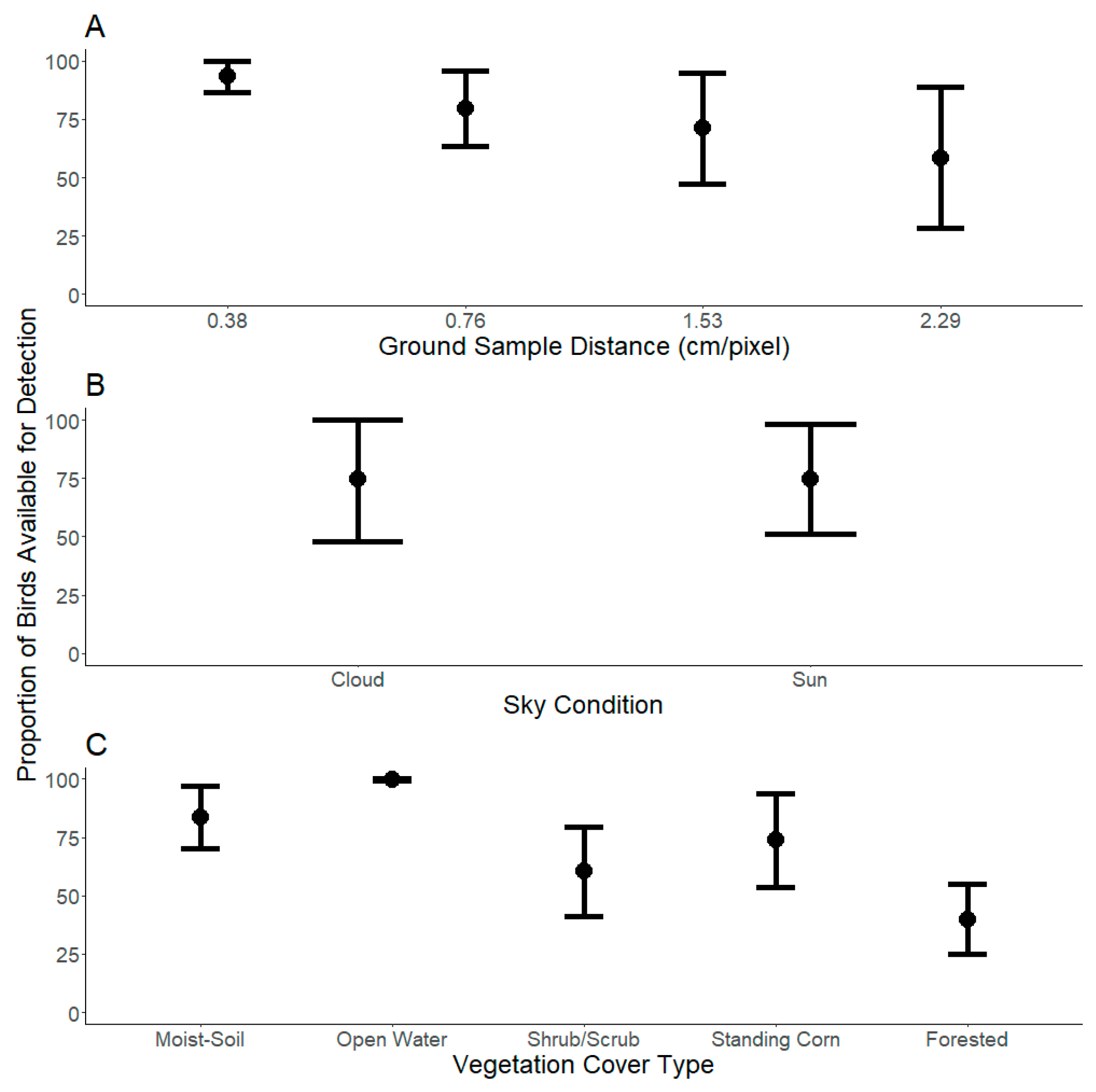
We collected 83 images of 14,940 individual decoys to evaluate the availability of waterfowl in UAS surveys across vegetation communities, sky conditions and GSD. The shrub–scrub vegetation cover type was not sampled under cloudy sky conditions due to time limitations and the forested vegetation cover type was not sampled at 0.38 cm/pixel GSD (survey altitudes of 15 m) due to the height of trees present in that cover type. For overall waterfowl availability, the interaction model was the best performing model (Table 1). The overall waterfowl availability in images decreased as the GSD increased (the survey altitude increased) and the vegetation-cover type became more complex, regardless of the sky conditions (Figure 2). For overall waterfowl availability, sky conditions alone had no effect on waterfowl availability (cloudy: mean = 74.66, 95% credible interval (CI) = 48.09–100.0, and sunny: mean = 74.61, 95% CI = 50.90–98.32), whereas increasing the complexity and height of the vegetation cover type decreased availability (Figure 2). Open water provided the most available waterfowl for sampling (mean = 99.78, 95% CI = 99.24–100.0), whereas moist soil (mean = 83.59, 95% CI = 70.18–97.00), standing corn (mean = 73.74, 95% CI = 53.73–93.77), and shrub–scrub (mean = 60.29, 95% CI = 41.05–79.52) all prevented more waterfowl from being sampled (Figure 2). The forested cover type precluded sampling the greatest number of waterfowl with only 39.90% (95% CI = 24.77–55.03) available for sampling (Figure 2). At a GSD of 1.53 cm/pixel (60 m, mean = 71.14, 95% CI = 47.41–94.85) and 2.29 cm/pixel (90 m, mean = 58.51, 95% CI = 28.12–88.90), waterfowl availability was lower than at a GSD of 0.38 (15 m, mean = 93.59, 95% CI = 86.59–100.0) while GSDs of 0.76 cm/pixel (30 m, mean = 79.51, 95% CI = 63.27–95.73) and 1.53 cm/pixel (60 m) were similar to each other (mean = 71.14, 95% CI = 47.41–94.85) (Figure 2).
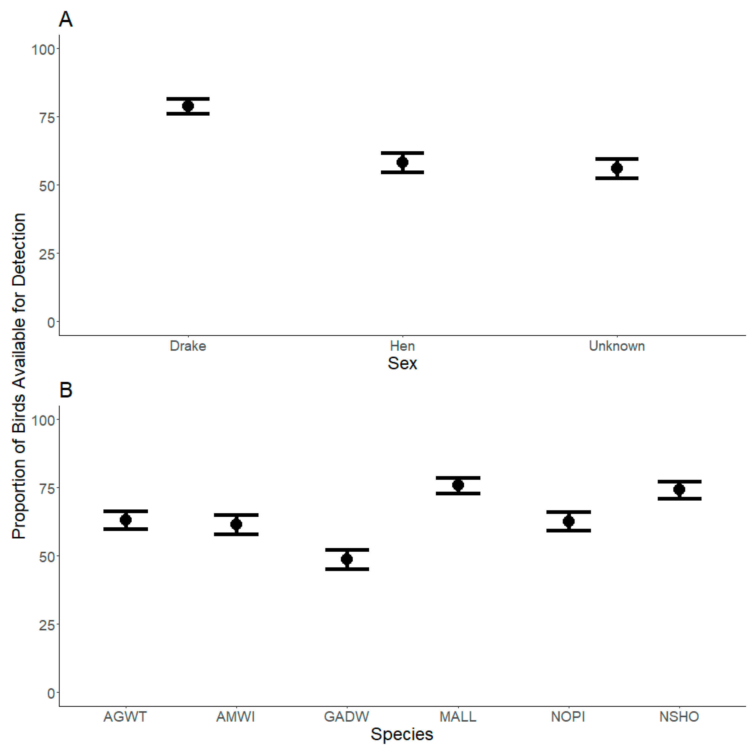
When we evaluated waterfowl availability by species and sex, the interaction model was the best performing model with the lowest WAIC (Table 1). Species- and sex-specific waterfowl availability was influenced most by vegetation cover type and GSD, whereas sky conditions did not have an influence on species- or sex-specific availability (Figure 3). Among species, mallards (mean = 75.77, 95% CI = 72.79–78.75) and northern shovelers (mean = 74.17, 95% CI = 71.10–77.23) had the highest sampling availability, with gadwall (mean = 48.83, 95% CI = 45.27–52.38) having the lowest availability (Figure 3). The availability of the American green-winged teal (mean = 63.13, 95% CI = 59.76–66.49), American wigeon (mean = 61.57, 95% CI = 59.76–65.07), and northern pintail (mean = 62.67, 95% CI = 59.20–66.14) was between the mallards/northern shovelers and the gadwall availability (Figure 3). Among all species, males (mean = 78.90, 95% CI = 76.13–81.67) had greater availability than females (mean = 58.18, 95% CI = 54.68–61.69) and unknown sex (mean = 55.98, 95% CI = 52.44–59.51) (Figure 3).

3.2. Perception Bias

We conducted 144 UAS flights over live birds at GSD of 0.38, 0.76, 1.53 (survey altitudes of 15, 30, and 60 m), collecting 404 images and 105,392 individual birds to evaluate the performance of artificial intelligence detection models for waterfowl counts. Shrub–scrub vegetation was not sampled under cloudy sky conditions due to time constraints, and for the forested vegetation cover type, the trees were taller than 15 m, so we were unable to conduct flights at 15 m. For both the probability that a bird was detected and the probability that a generated algorithm detection was a false positive, the interaction models performed the best with the lowest WAIC, indicating that the combination of GSD, sky condition, and vegetation cover type influences algorithm detections (Table 2).
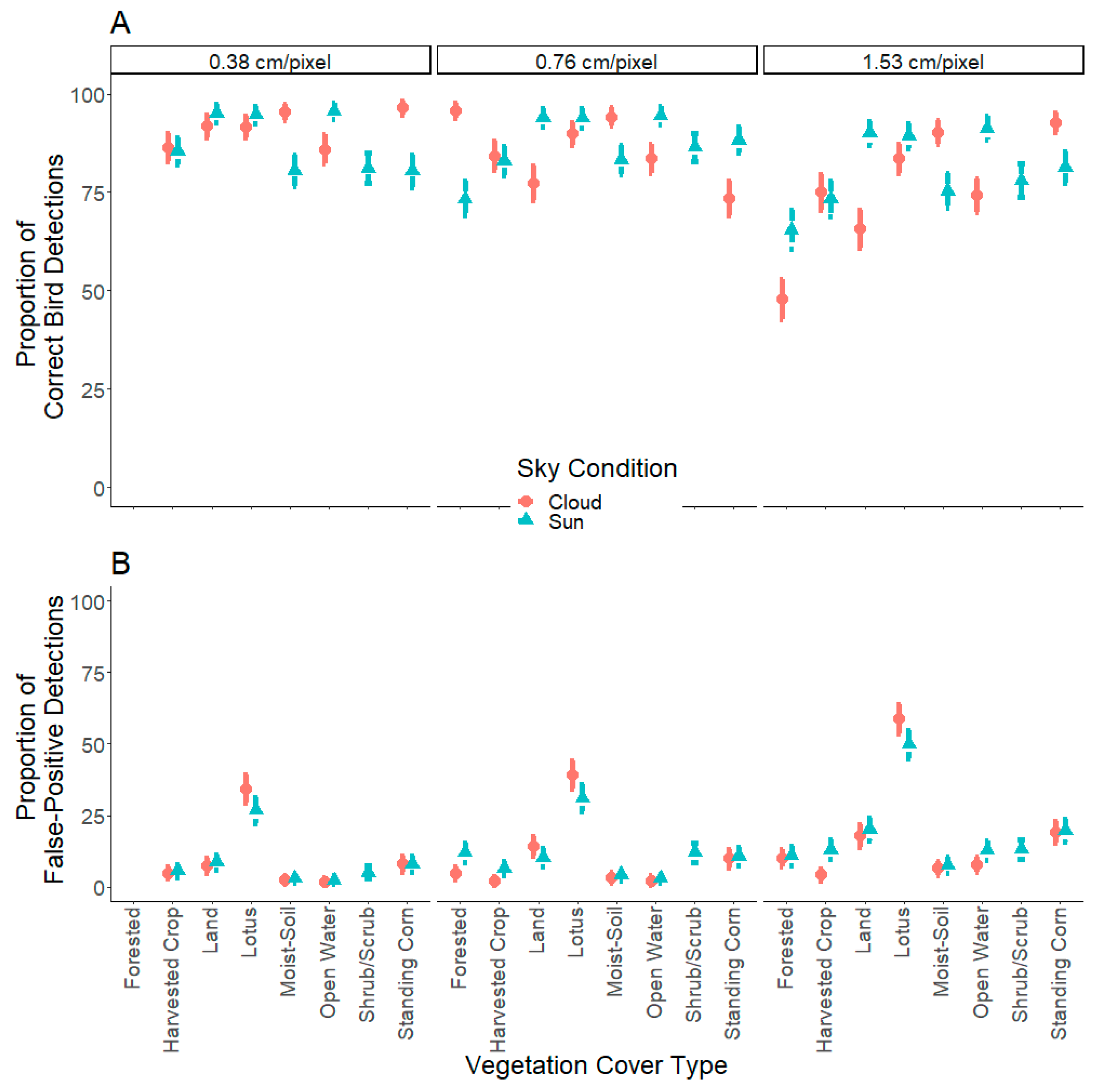
The probability that a bird was detected by the algorithm differed among some vegetation cover types, with a lower detection probability in shrub–scrub (mean = 81.64, 95% CI = 76.38–86.91) compared to the two vegetation cover types with greatest bird detection probability estimates: lotus (mean = 90.50, 95% CI = 85.75–95.25) and open water (mean = 87.58, 95% CI = 79.44–95.72) (Figure 4). The bird detection probability was lower in forested (mean = 70.58, 95% CI = 52.86–88.31) and harvested crop (mean = 81.30, 95% CI = 74.77–87.84) vegetation cover types compared to lotus, and there were no differences in bird detection probability among the other vegetation-cover types (standing corn: mean = 85.51, 95% CI = 76.95–94.06, land: mean = 85.70, 95% CI = 74.54–96.87, and moist soil: mean = 86.55, 95% CI = 78.55–94.55) (Figure 4). The probability that a bird was detected by the algorithm was not individually influenced by GSD (15 m: mean = 89.29, 95% CI = 82.58–96.00, 30 m: mean = 86.39, 95% CI = 78.30–94.49, 60 m: mean = 78.23, 95% CI = 65.68–90.78) or sky condition (cloudy: mean = 83.79, 95% CI = 71.48–96.11, and sunny: mean = 84.91, 95% CI = 76.06–93.88) (Figure 4). Interactively, the combination of forested vegetation cover type, cloudy sky conditions, and a GSD of 1.53 cm/pixel (60 m) had a significantly lower bird detection probability than all other combinations (mean = 47.89, 95% CI = 42.65–53.12) (Figure 5).
More false-positives were generated in the vegetation cover types that had features similar in size and shape to the birds, with significantly more false positive detections for lotus (mean = 39.99, 95% CI = 27.88–52.10) compared to the other vegetation cover types (Figure 4). Interactively, the combination of lotus vegetation cover type, cloudy sky conditions, and a GSD of 60 m showed significantly more false-positive detections than all other combinations (mean = 58.74, 95% CI = 53.70–63.78), with the combinations of both sky conditions and other GSD over the lotus vegetation cover type all producing a significantly greater proportion of false-positive detections than other combinations of vegetation cover type, sky condition, and GSD (Figure 5).The probability that a generated algorithm detection was a false positive was not individually influenced by GSD (15 m: mean = 9.13, 95% CI = 0.00–19.04, 30 m: mean = 11.05, 95% CI = 0.31–21.78, 60 m: mean = 18.09, 95% CI = 2.60–33.58) or sky condition (cloudy: mean = 12.97, 95% CI = 0.00–27.78, and sunny: mean = 12.89, 95% CI = 1.75–24.03) (Figure 4).

3.3. Correcting Image Counts

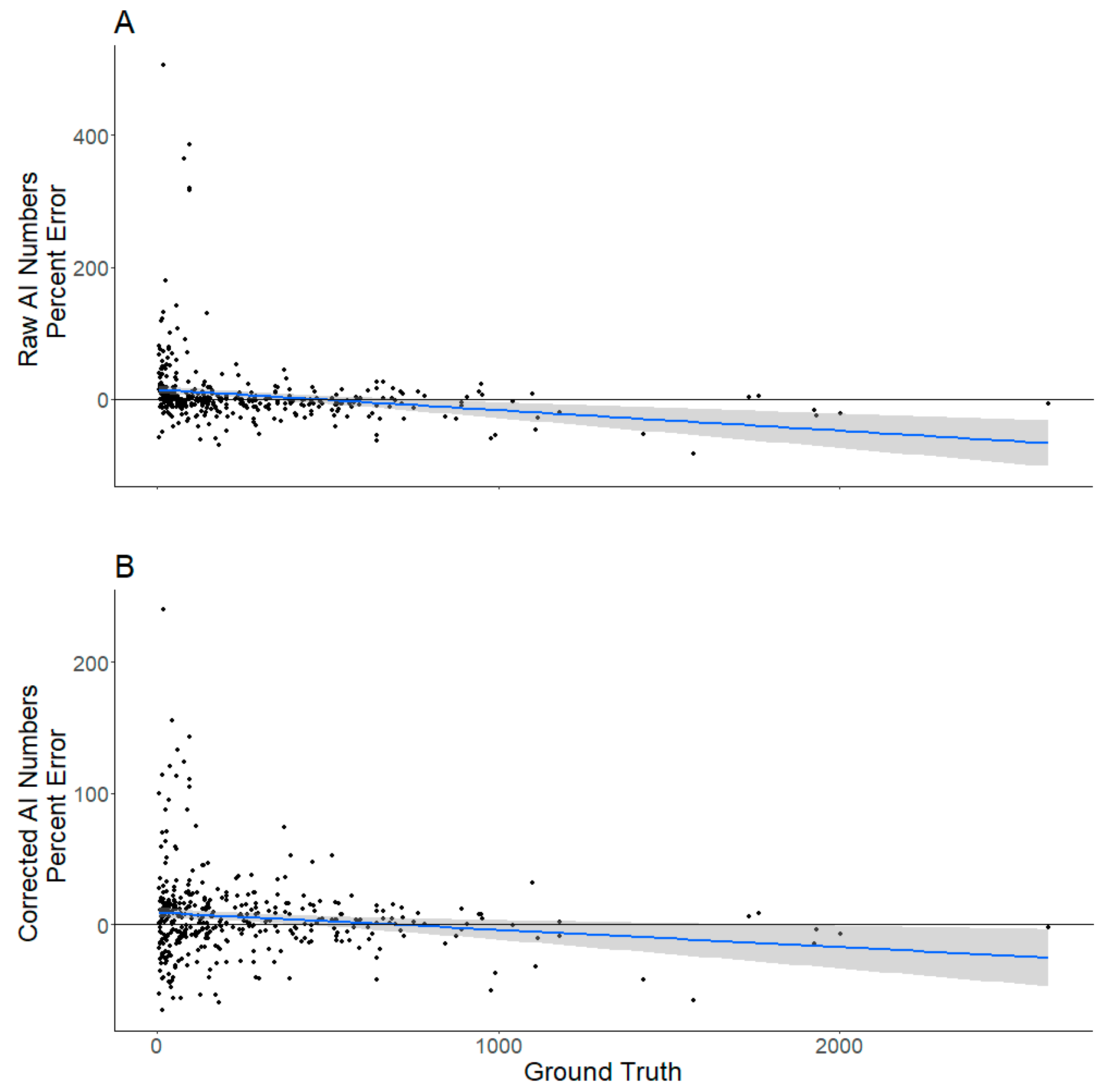
To evaluate the accuracy of correcting artificial intelligence to estimate the true number of birds in the image, we used five images for each vegetation cover type, sky condition, and GSD, that were not used in training or testing the algorithms or in fitting our models to estimate detection probabilities (n = 215 labeled images and 58,943 birds).Our modified H–T estimator counts resulted in a mean absolute error of 38.51 birds per image from the human label ground truths (3.35% ± 0.08 lower than the ground truth) compared to the uncorrected raw algorithm outputs with a mean absolute error of 47.16 birds per image (6.70% ± 0.13 higher than the ground truth) (Figure 6 and Figure 7). As the GSD increased, the corrected algorithm counts percent error increased from 0.557 percent (SE ± 0.15) at a GSD of 0.38 cm/pixel (15 m) to 12.8 percent (SE ± 0.37) at 1.53 cm/pixel (60 m) with 3.95 percent error (SE ± 0.17) at 0.76 cm/pixel (30 m). The raw algorithm counts had 0.720 percent (SE ± 0.19) error at a GSD of 0.38 cm/pixel (15 m) and 19.6 percent (SE ± 0.68) error at 1.53 cm/pixel (60 m) with 1.06 percent (SE ± 0.17) error at 0.76 cm/pixel (30 m) (Figure 6). Across vegetation cover types, the percent error ranged from −0.313 percent (SE ± 0.92) in lotus to 10.4 percent (SE ± 0.59) in standing corn for the corrected algorithm counts compared to 58.4 percent (SE ± 1.85) in lotus to 6.99 percent (SE ± 0.51) in standing corn for the raw algorithm counts (Figure 6). The algorithm performed best in open water, with an average percent error of -2.17 percent (SE ± 0.35) compared to the corrected counts of 5.78 percent (SE ± 0.31) (Figure 7). Within the two sky conditions, the corrected counts in sunny conditions produced less error (4.04 percent [SE ± 0.14]) than the cloudy conditions (7.42 percent [SE ± 0.19]), and overall, the corrected counts were more accurate than the raw algorithm counts in sunny (4.30 percent [SE ± 0.20]) and cloudy (9.54 percent [SE ± 0.33]) conditions (Figure 6). Overall, the linear model used to represent the correction ratio between corrected counts and human labeled counts had a slope of 0.97 (SE ± 0.01) with an adjusted R2 of 0.96 compared to a slope of 0.88 (SE ± 0.01) with an adjusted R2 of 0.93 for the raw algorithm counts (Figure 7).

4. Discussion

Overall, our results show that UASs, aerial imagery, artificial intelligence algorithms, and the use of correction factors may accurately estimate waterfowl abundance within single images across a wide range of environmental and flight conditions. Previous studies evaluating bird detection biases found that vegetation cover type, sky condition, species, and survey altitude or GSD can all influence bird detection within a survey area [20,36,37,38,39,42,43]. We found that waterfowl availability bias was most influenced by environmental conditions, including vegetation cover type, GSD, and waterfowl characteristics, including species and sex, while perception bias was most influenced by GSD, affecting the probability of detecting birds, and vegetation-cover type, influencing the probability of algorithms generating false positives. By separating availability and perception bias, our use of the modified H–T estimator to correct for biases increases the accuracy of bird abundance estimates, with overall correction factors ranging from 1.0 to 6.5 depending on vegetation cover type, GSD, and waterfowl species and sex. The use of these correction factors from the modified H–T estimator reduced waterfowl count error in individual images by half, from 6.70 percent to 3.35 percent across all vegetation cover types, sky condition, GSD, and waterfowl species and sex.

4.1. Availability Bias

Previous studies using remote sensing found that vegetation cover type, sky condition, species, and survey altitude or GSD can all influence waterfowl detection within a survey area [20,36,37,38,39,42,43]. Similarly, our results indicate that in UAS imagery, the waterfowl availability to be counted was strongly influenced by the combination of species, sex, vegetation cover type, and GSD. Unlike previous studies, we found that sky condition did not have a strong effect on availability. Similar to previous studies using UAS or human observers, increasing the complexity and vertical component of vegetation reduced the availability of waterfowl in the images, with forested vegetation communities reducing the waterfowl availability the most [35,37,38,39]. Waterfowl availability was likely reduced in the forested vegetation cover type due to larger branches covering birds and the vertical component of the tree trunks obscuring large parts around the edges of the images where the view angle was wider as compared to the middle of the images where the view was straight down [61,62,63]. The vertical components of the moist soil, standing corn, and shrub–scrub vegetation cover types were less extensive than in the forested vegetation cover type, so we did not see the edge effects in these other vegetation communities, allowing waterfowl to be more available throughout the entire images [33,39]. Thus, despite birds still being covered by vegetation in these other vegetation types, more of the birds were available throughout the image [38,39]. If the image size in the forested vegetation cover type was reduced, such that only the center portion of each image was sampled and used as the sampling footprint, a higher percentage of birds may be available for counting. This would be similar to similar to reducing the width of transects for ocular aerial survey in forested communities, restricting the view to straight down, allowing for higher waterfowl availability [61,62,63].
Our observed waterfowl availability patterns followed previous studies evaluating ground sampling distances and waterfowl availability or count accuracy, with availability and accuracy decreasing as the ground sampling distance increased [27,29,43]. We found that the overall availability decreased at a GSD of 1.53 and 2.29 cm/pixel (60 and 90 m) relative to 0.38 and 0.76 cm/pixel (15 and 30 m). In our study, it was difficult to discern whether the decrease in availability with increasing GSD and altitude was due to a loss of spatial resolution and therefore information, or if it was due to the birds appearing to be more covered by vegetation and less visible to the camera. Waterfowl availability in open water did decrease slightly as GSD increased, suggesting a component of spatial resolution loss contributing to the lower availability at higher GSD; however, the availability of waterfowl in the other vegetation communities decreased more than expected based on the open water availability at the higher GSD [27,29,43]. Alternatively, birds were more likely to be obscured by vegetation in the other vegetation cover types, and thus as GSD was reduced with increasing altitude, the proportion of the bird required for successful identification was larger, and in the more complex vegetation communities there were less of these larger portions of birds visible, thus reducing the availability more than the decrease shown in the open water communities [37,38,39].
The plumage characteristics of the birds themselves from species- and sex-dependent coloration overall influenced waterfowl availability, with darker and more plain-colored birds (hens and GADW) having reduced availability compared to birds with more colorful plumage (drakes) [42,43]. The drab coloration of hens and GADW matched the vegetation surrounding the birds, making it challenging to confidently discern between those birds and the vegetation, unlike the drakes with distinguishing coloration features in the same situation. We found no difference in waterfowl availability between sunny or cloudy conditions, regardless of plumage patterns, whereas previous studies have shown that sunlight may reduce availability of lighter-colored individuals [26,40,41,42]. Although most drakes contained some white plumage, it was not enough to reduce availability compared to hens in sunny conditions. This pattern was also observed when comparing availability among species, with lighter-colored species showing no difference in availability compared to darker species in sunny conditions.
Interestingly, we found bird body size was not important for determining availability, as AGWT, our smallest decoys, had similar availability to AMWI and NOPI, and better availability than GADW, while MALL, our largest decoys, did not have better availability than NSHO. This result was surprising, as it would be expected that larger birds are more available than smaller birds. Similar to previous studies, we found that the species- and sex-specific identification probability decreased from a GSD of 0.38 cm/pixel to 0.76 cm/pixel (15 and 30 m, respectively), and it was nearly impossible to confidently identify individuals to species and sex on imagery collected (>1.0 cm/pixel (>45 m) [27,29,43]. Other studies have shown that reductions in species-specific identification were due to an increase in GSD rather than other factors, such as changes in lighting or the appearance of vegetation communities at different altitudes [27,43]. The increase in GSD leads to a loss of species- or sex-specific coloration patterns, and improvements in camera technologies will eventually overcome this barrier, allowing for improved capacity for species- or sex-specific identification during higher surveys.

4.2. Perception Bias

Previous studies found that vegetation cover type, sky condition, and GSD all influence the detection of avifauna by machine-learning algorithms in aerial imagery [26,30,31,32,35]. In our study, the probability of a bird being detected by the machine-learning algorithm and the probability that an algorithm detection was a false positive were both influenced by the combination of GSD (survey altitude), sky condition, and vegetation cover type. Although increasing the complexity of the vegetation cover type did not influence the algorithm’s detection of birds, the presence of vegetation-cover types that had features similar in size and shape to the birds, such as lotus, significantly increased the probability of the algorithm generating a false-positive detection. Aside from the lotus vegetation-cover type, the lack of vegetation-cover type influences on the algorithm detecting birds or generating false positives may be due to the training of algorithms on images collected on waterfowl under the same specific conditions, creating robust algorithms for our specific scenarios. These results indicate that algorithm performance may improve with additional training on more scenarios including lotus. Future algorithms will likely achieve the best possible algorithm performance if robustly trained on example images for every vegetation cover type expected in surveys [31,32,35,44,45].
Unlike findings from previous studies, differences in sky condition or increasing GSD did not decrease the probability of detecting a bird or increase the probability of an algorithm detection being a false positive [21,26,42]. Previous studies reported sunlight may reduce detection, especially of lighter-colored objects; however, we did not evaluate the algorithm’s success at detecting individual species or sexes; rather, we focused on detection of overall species and sexes combined, thus potentially losing some of the impact of those interactions between species, sex, and sky condition [21,26,31,37,43]. We also found no influence of GSD (or survey altitude) on the detection probability of birds from the algorithms, unlike previous studies that found count accuracy decreased as GSD or altitude increased. We only evaluated the algorithms on images collected up to 1.53 cm/pixel (60 m) due to the significant portion of birds that were unavailable for surveying at 2.29 cm/pixel (90 m) and loss of resolution to manually label birds. Previous studies also found that between 1.5 and 2.0 cm/pixel, the success of the algorithm detecting waterfowl significantly decreases [23,24,27,29,43]. Although previous studies have found the physical characteristics of the birds themselves (species- and sex-dependent coloration) influenced the availability and algorithm detection of waterfowl, we were unable to evaluate the success of detection by species or sex of waterfowl due to limitations related to labeling birds to the species and sex level in our dataset [26,37,42,43]. The loss of spatial resolution leads to a loss of species- or sex-specific coloration patterns, and improvements in camera technologies will likely overcome this barrier, allowing for species- or sex-specific identification during higher surveys [20,21,31,32,35,44].
We also acknowledge that our annotation methods resulted in two sources of errors. The first source of error was caused by our choice to only label birds that were completely contained within the image (whole birds). We did this to prevent the algorithm from identifying each part of a bird as a separate bird and therefore counting them twice. While evaluating the algorithm, we again only used labeled images in which entire birds were labeled and the partial birds around image edges were not labeled. This potentially caused partial birds around the edges of the images to be detected by the algorithm, and although they were correctly identified, they are considered false positives in our evaluation because they do not match a ground-truth label of a bird. We estimate these errors accounted for up to 5% of the false-positive detections, with most images experiencing 0–3% of false positives occurring from this labeling error. Second, we cropped large images into smaller images to improve the speed of labeling and then stitched these small images back together after they were labeled. During the stitching process, some bounding boxes on the same bird did not meet the overlap requirement to be considered as belonging to one bird, causing us to retain both labels as if they were two individual birds. These errors may have occurred for up to five percent of the labels, causing between zero and three percent error in the evaluation of the algorithm detecting birds. These labeling errors are challenging to address and likely to have minimal effect on the results of detection probabilities from the algorithms (up to five percent error for false positives and five percent error for detection of a bird) and are therefore unlikely to influence the correction factors used to correct the raw algorithm counts to the true number of birds likely to be in the image.

4.3. Correcting Image Counts

Incorporating algorithm detection probabilities to correct for biases may increase the accuracy of bird abundance estimates, although there has been limited effort to correct artificial intelligence algorithm counts of animals in aerial imagery [47,48,49]. In our study, correction factors accounting for vegetation cover type, sky condition, and GSD range from 1.10 in open water to 3.20 in forested vegetation at 0.76 cm/pixel (30 m) on cloudy days. Across all GSDs, sky conditions, and vegetation cover types, correction factors range from 1.0 to 6.5, which are better than visual correction factors in ocular aerial surveys, ranging from 2.5 to 8.8 [61,62,63]. Looking at count accuracy on a per-image basis, the modified H–T estimator corrections reduced the count error from 6.70 percent to 3.35 percent across all vegetation-cover types and GSD. The effect of correcting algorithm counts increased as altitude increased and correcting the counts in images taken at a GSD of 1.53 cm/pixel (60 m) improved the accuracy more than at the lower GSD. We observed similar trends among different vegetation-cover types, where correcting counts improved accuracy by 58 percent in the more problematic cover types such as lotus, whereas corrections decreased the accuracy of counts in open water by 3 percent.

4.4. Management Implications

Overall, our results show that while the artificial intelligence algorithms can accurately detect and estimate waterfowl abundance within single images across a wide range of environmental and flight conditions, the waterfowl’s availability to be counted in the images is often dependent on environmental conditions. Thus, flights conducted during times in which waterfowl are more available for surveying are likely to provide more precise and accurate abundance estimates. The use of developed algorithms may work well under most conditions to provide accurate estimates of the number of waterfowl present in an image without the need for correction factors or other methods of correcting the algorithm’s counts to produce accurate estimates. However, in surveys with more challenging conditions for bird detection, such as in lotus vegetation cover types, correcting or adjusting the algorithm numbers is critical to improve accuracy of abundance estimates. If managers decide that abundance estimates obtained under certain conditions are sufficiently accurate, they may be able to save time by using the uncorrected algorithm estimates from the images instead of spending the extra time and money required to run corrections on the algorithm outputs. More research is needed to evaluate other methods of evaluating detection and adjusting waterfowl abundance estimates, both on a per-image basis for evaluating artificial intelligence algorithms, and on a landscape or survey unit scale to determine the best survey methodology that provides accurate and precise abundance estimates for an entire conservation area or refuge.

Author Contributions

Conceptualization, A.R. and E.W.; methodology, A.R., E.W. and R.V.; software, Z.T., Y.Z., Z.Z., Z.L., S.W. and J.Z.; validation, A.R. and E.W.; formal analysis, R.V.; investigation, A.R. and E.W.; resources, Z.T., Y.Z. and S.W.; data curation, R.V., Z.T., Y.Z. and S.W.; writing—original draft preparation, R.V.; writing—review and editing, A.R., E.W. and R.V.; visualization, R.V.; supervision, E.W.; project administration, E.W.; funding acquisition, A.R., E.W. and Y.S. All authors have read and agreed to the published version of the manuscript.

Funding

This research was funded by the Missouri Department of Conservation through Cooperative Agreement #433.

Data Availability Statement

Data are not currently available from funding organization Missouri Department of Conservation. Contact the Missouri Department of Conservation for further information.

Acknowledgments

We thank MDC wetland managers B. Anderson, B. Lichtenberg, C. Crisler, J. Marshall, L. Wehmhoff, N. Walker, R. Henry, R. Kelly, S. Allen, T. Kavan, and T. Tallman, for providing access and allowing us to conduct UAS flights on the wetlands. The Missouri Cooperative Fish and Wildlife Research Unit is jointly sponsored by the Missouri Department of Conservation, the University of Missouri, the U.S. Fish and Wildlife Service, the U.S. Geological Survey, and the Wildlife Management Institute. Use of trade, product, or firm names is for descriptive purposes only and does not imply U.S. Government endorsement.

Conflicts of Interest

The authors declare no conflicts of interest. The funders had no role in the design of the study; in the collection, analyses, or interpretation of data; in the writing of the manuscript; or in the decision to publish the results.

References

  1. Nichols, J.; Johnson, F.; Williams, B. Managing North American waterfowl in the face of uncertainty. Annu. Rev. Ecol. Syst. 1995, 26, 177–199. [Google Scholar] [CrossRef]
  2. Williams, B.; Johnson, F. Adaptive management and the regulation of waterfowl harvests. Wildl. Soc. Bull. 1995, 23, 430–436. [Google Scholar]
  3. Rönkä, M.; Saari, L.; Hario, M.; Hänninen, J.; Lehikoinen, E. Breeding success and breeding population trends of waterfowl: Implications for monitoring. Wildl. Biol. 2011, 17, 225–239. [Google Scholar] [CrossRef] [PubMed]
  4. Soulliere, G.; Loges, B.; Dunton, E.; Luukkonen, D.; Eichholz, M.; Koch, M. Monitoring waterfowl in the Midwest during the non-breeding period: Challenges, priorities, and recommendations. J. Fish Wildl. Manag. 2013, 4, 395–405. [Google Scholar] [CrossRef]
  5. Hagy, H. Coordinated Aerial Waterfowl Surveys on National Wildlife Refuges in the Southeast during Winter 2020; U.S. Fish and Wildlife Service Report, U.S. Fish and Wildlife Service; 2020. Available online: https://ecos.fws.gov/ServCat/DownloadFile/173701 (accessed on 6 June 2023).
  6. Davis, K.; Silverman, E.; Sussman, A.; Wilson, R.; Zipkin, E. Errors in aerial survey count data: Identifying pitfalls and solutions. Ecol. Evol. 2022, 12, e8733. [Google Scholar] [CrossRef]
  7. Pagano, A.; Arnold, T. Estimating detection probabilities of waterfowl broods from ground-based surveys. J. Wildl. Manag. 2009, 73, 686–694. [Google Scholar] [CrossRef]
  8. Eggeman, D.; Johnson, F. Variation in effort and methodology for the midwinter waterfowl inventory in the Atlantic Flyway. Wildl. Soc. Bull. (1973–2006) 1989, 17, 227–233. [Google Scholar]
  9. Nichols, T.; Clark, L. Comparison of Ground and Helicopter Surveys for Breeding Waterfowl in New Jersey. Wildl. Soc. Bull. 2021, 45, 508–516. [Google Scholar] [CrossRef]
  10. Smith, G. A Critical Review of the Aerial and Ground Surveys of Breeding Waterfowl in North America; US Department of the Interior, National Biological Service: Washington, DC, USA, 1995; Volume 5.
  11. Sasse, D. Job-related mortality of wildlife workers in the United States, 1937–2000. Wildl. Soc. Bull. 2003, 31, 1015–1020. [Google Scholar]
  12. Kumar, A.; Rice, M. Optimized Survey Design for Monitoring Protocols: A Case Study of Waterfowl Abundance. J. Fish Wildl. Manag. 2021, 12, 572–584. [Google Scholar] [CrossRef]
  13. Leedy, D. Aerial photographs, their interpretation and suggested uses in wildlife management. J. Wildl. Manag. 1948, 12, 191–210. [Google Scholar] [CrossRef]
  14. Leonard, R.; Fish, E. An aerial photographic technique for censusing lesser sandhill cranes. Wildl. Soc. Bull. 1974, 2, 191–195. [Google Scholar]
  15. Ferguson, E.; Jorde, D.; Sease, J. Use of 35-mm color aerial photography to acquire mallard sex ratio data. Photogramm. Eng. Remote Sens. 1981, 47, 823–827. [Google Scholar]
  16. Haramis, G.; Goldsberry, J.; McAuley, D.; Derleth, E. An aerial photographic census of Chesapeake Bay and North Carolina canvasbacks. J. Wildl. Manag. 1985, 49, 449–454. [Google Scholar] [CrossRef]
  17. Cordts, S.; Zenner, G.; Koford, R. Comparison of helicopter and ground counts for waterfowl in Iowa. Wildl. Soc. Bull. 2002, 30, 317–326. [Google Scholar]
  18. Anderson, K.; Gatson, K. Lightweight unmanned aerial vehicles will revolutionize spatial ecology. Front. Ecol. Environ. 2013, 11, 138–146. [Google Scholar] [CrossRef] [PubMed]
  19. Gonzalez, L.; Montes, G.; Puig, E.; Johnson, S.; Mengersen, K.; Gaston, K. Unmanned aerial vehicles (UAVs) and artificial intelligence revolutionizing wildlife monitoring and conservation. Sensors 2016, 16, 97. [Google Scholar] [CrossRef] [PubMed]
  20. Wang, D.; Shao, Q.; Yue, H. Surveying wild animals from satellites, manned aircraft and unmanned aerial systems (UASs): A review. Remote Sens. 2019, 11, 1308. [Google Scholar] [CrossRef]
  21. Dundas, S.; Vardanega, M.; O’Brien, P.; McLeod, S. Quantifying waterfowl numbers: Comparison of drone and ground-based survey methods for surveying waterfowl on artificial waterbodies. Drones 2021, 5, 5. [Google Scholar] [CrossRef]
  22. Scholten, C.; Kamphuis, A.; Vredevoogd, K.; Lee-Strydhorst, K.; Atma, J.; Shea, C.; Lamberg, O.; Proppe, D. Real-time thermal imagery from an unmanned aerial vehicle can locate ground nests of a grassland songbird at rates similar to traditional methods. Biol. Conserv. 2019, 233, 241–246. [Google Scholar] [CrossRef]
  23. Tang, Z.; Zhang, Y.; Wang, Y.; Shang, Y.; Viegut, R.; Webb, E.; Raedeke, A.; Sartwell, J. sUAS and Machine Learning Integration in Waterfowl Population Surveys. In Proceedings of the 2021 IEEE 33rd International Conference on Tools with Artificial Intelligence (ICTAI), Virtual Conference, 1–3 November 2021; IEEE: Piscataway, NJ, USA, 2021; pp. 517–521. [Google Scholar]
  24. Zhang, Y.; Wang, S.; Zhai, Z.; Shang, Y.; Viegut, R.; Webb, E.; Raedeke, A.; Sartwell, J. Development of New Aerial Image Datasets and Deep Learning Methods for Waterfowl Detection and Classification. In Proceedings of the 2022 IEEE 4th International Conference on Cognitive Machine Intelligence (CogMI), Atlanta, GA, USA, 14–17 December 2022; IEEE: Piscataway, NJ, USA, 2022; pp. 117–124. [Google Scholar]
  25. Lawrence, B.; de Lemmus, E.; Cho, H. UAS-Based Real-Time Detection of Red-Cockaded Woodpecker Cavities in Heterogeneous Landscapes Using YOLO Object Detection Algorithms. Remote Sens. 2023, 15, 883. [Google Scholar] [CrossRef]
  26. Chabot, D.; Dillon, C.; Francis, C. An approach for using off-the-shelf object-based image analysis software to detect and count birds in large volumes of aerial imagery. Avian Conserv. Ecol. 2018, 13, 15. [Google Scholar] [CrossRef]
  27. Hodgson, J.; Mott, R.; Baylis, S.; Pham, T.; Wotherspoon, S.; Kilpatrick, A.; Segaran, R.; Reid, I.; Terauds, A.; Koh, L. Drones count wildlife more accurately and precisely than humans. Methods Ecol. Evol. 2018, 9, 1160–1167. [Google Scholar] [CrossRef]
  28. Wen, D.; Su, L.; Hu, Y.; Xiong, Z.; Liu, M.; Long, Y. Surveys of large waterfowl and their habitats using an unmanned aerial vehicle: A case study on the Siberian crane. Drones 2021, 5, 102. [Google Scholar] [CrossRef]
  29. Dulava, S.; Bean, W.; Richmond, O. Environmental reviews and case studies: Applications of unmanned aircraft systems (UAS) for waterbird surveys. Environ. Pract. 2015, 17, 201–210. [Google Scholar] [CrossRef]
  30. Kellenberger, B.; Tuia, D.; Morris, D. AIDE: Accelerating image-based ecological surveys with interactive machine learning. Methods Ecol. Evol. 2020, 11, 1716–1727. [Google Scholar] [CrossRef]
  31. Kabra, K.; Xiong, A.; Li, W.; Luo, M.; Lu, W.; Yu, T.; Yu, J.; Singh, D.; Garcia, R.; Tang, M.; et al. Deep object detection for waterbird monitoring using aerial imagery. In Proceedings of the 2022 21st IEEE International Conference on Machine Learning and Applications (ICMLA), Nassau, Bahamas, 12–14 December 2022; IEEE: Piscataway, NJ, USA, 2022; pp. 455–460. [Google Scholar]
  32. Weinstein, B.; Garner, L.; Saccomanno, V.; Steinkraus, A.; Ortega, A.; Brush, K.; Yenni, G.; McKellar, A.; Converse, R.; Lippitt, C.; et al. A general deep learning model for bird detection in high-resolution airborne imagery. Ecol. Appl. 2022, 32, e2694. [Google Scholar] [CrossRef]
  33. Pöysä, H.; Kotilainen, J.; Väänänen, V.; Kunnasranta, M. Estimating production in ducks: A comparison between ground surveys and unmanned aircraft surveys. Eur. J. Wildl. Res. 2018, 64, 74. [Google Scholar] [CrossRef]
  34. Willi, M.; Pitman, R.; Cardoso, A.; Locke, C.; Swanson, A.; Boyer, A.; Veldthuis, M.; Fortson, L. Identifying animal species in camera trap images using deep learning and citizen science. Methods Ecol. Evol. 2019, 10, 80–91. [Google Scholar] [CrossRef]
  35. Tuia, D.; Kellenberger, B.; Beery, S.; Costelloe, B.; Zuffi, S.; Risse, B.; Mathis, A.; Mathis, M.; van Langevelde, F.; Burghardt, T.; et al. Perspectives in machine learning for wildlife conservation. Nat. Commun. 2022, 13, 792. [Google Scholar] [CrossRef]
  36. Liu, Y.; Sun, P.; Highsmith, M.; Wergeles, N.; Sartwell, J.; Raedeke, A.; Mitchell, M.; Hagy, H.; Gilbert, A.; Lubinski, B.; et al. Performance comparison of deep learning techniques for recognizing birds in aerial images. In Proceedings of the 2018 IEEE Third International Conference on Data Science in Cyberspace (DSC), Guangzhou, China, 18–21 June 2018; IEEE: Piscataway, NJ, USA, 2018; pp. 317–324. [Google Scholar]
  37. Barr, J.; Green, M.; DeMaso, S.; Hardy, T. Detectability and visibility biases associated with using a consumer-grade unmanned aircraft to survey nesting colonial waterbirds. J. Field Ornithol. 2018, 89, 242–257. [Google Scholar] [CrossRef]
  38. Bushaw, J.; Ringelman, K.; Johnson, M.; Rohrer, T.; Rohwer, F. Applications of an unmanned aerial vehicle and thermal-imaging camera to study ducks nesting over water. J. Field Ornithol. 2020, 91, 409–420. [Google Scholar] [CrossRef]
  39. Bushaw, J.; Terry, C.; Ringelman, K.; Johnson, M.; Kemink, K.; Rohwer, F. Application of unmanned aerial vehicles and thermal imaging cameras to conduct duck brood surveys. Wildl. Soc. Bull. 2021, 45, 274–281. [Google Scholar] [CrossRef]
  40. Marchowski, D. Drones, automatic counting tools, and artificial neural networks in wildlife population censusing. Ecol. Evol. 2021, 11, 16214. [Google Scholar] [CrossRef]
  41. Elmore, J.; Schultz, E.; Jones, L.; Evans, K.; Samiappan, S.; Pfeiffer, M.; Blackwell, B.; Iglay, R. Evidence on the efficacy of small unoccupied aircraft systems (UAS) as a survey tool for North American terrestrial, vertebrate animals: A systematic map. Environ. Evid. 2023, 12, 3. [Google Scholar] [CrossRef]
  42. Francis, R.; Lyons, M.; Kingsford, R.; Brandis, K. Counting mixed breeding aggregations of animal species using drones: Lessons from waterbirds on semi-automation. Remote Sens. 2020, 12, 1185. [Google Scholar] [CrossRef]
  43. Burr, P.; Samiappan, S.; Hathcock, L.; Moorhead, R.; Dorr, B. Estimating Waterbird Abundance on Catfish Aquaculture Ponds Using an Unmanned Aerial System; USDA National Wildlife Research Center—Staff Publications: Fort Collins, CO, USA, 2019; p. 2302.
  44. Wu, E.; Wang, H.; Lu, H.; Zhu, W.; Jia, Y.; Wen, L.; Choi, C.-Y.; Guo, H.; Li, B.; Sun, L.; et al. Unlocking the Potential of Deep Learning for Migratory Waterbirds Monitoring Using Surveillance Video. Remote Sens. 2022, 14, 514. [Google Scholar] [CrossRef]
  45. Lyons, M.; Brandis, K.; Murray, N.; Wilshire, J.; McCann, J.; Kingsford, R.; Callaghan, C. Monitoring large and complex wildlife aggregations with drones. Methods Ecol. Evol. 2019, 10, 1024–1035. [Google Scholar] [CrossRef]
  46. Marsh, H.; Sinclair, D. Correcting for visibility bias in strip transect aerial surveys of aquatic fauna. J. Wildl. Manag. 1989, 53, 1017–1024. [Google Scholar] [CrossRef]
  47. Eikelboom, J.; Wind, J.; van de Ven, E.; Kenana, L.; Schroder, B.; de Knegt, H.; van Langevelde, F.; Prins, H. Improving the precision and accuracy of animal population estimates with aerial image object detection. Methods Ecol. Evol. 2019, 10, 1875–1887. [Google Scholar] [CrossRef]
  48. Augustine, B.; Koneff, M.; Pickens, B.; Royle, J. Towards estimating marine wildlife abundance using aerial surveys and deep learning with hierarchical classifications subject to error. bioRxiv 2023, 2023-02. [Google Scholar]
  49. Corcoran, E.; Denman, S.; Hamilton, G. New technologies in the mix: Assessing N-mixture models for abundance estimation using automated detection data from drone surveys. Ecol. Evol. 2020, 10, 8176–8185. [Google Scholar] [CrossRef]
  50. Hong, S.; Han, Y.; Kim, S.; Lee, A.; Kim, G. Application of deep-learning methods to bird detection using unmanned aerial vehicle imagery. Sensors 2019, 19, 1651. [Google Scholar] [CrossRef]
  51. Steinhorst, R.; Samuel, M. Sightability adjustment methods for aerial surveys of wildlife populations. Biometrics 1989, 45, 415–425. [Google Scholar] [CrossRef]
  52. Gabor, T.; Gadawski, T.; Ross, R.; Rempel, R.; Kroeker, D. Visibility Bias of Waterfowl Brood Surveys Using Helicopters in the Great Clay Belt of Northern Ontario (Vicios en la Visibilidad de Camadas de Aves Acuáticas Durante Muestreos Que Usen Helicópteros). J. Field Ornithol. 1995, 66, 81–87. [Google Scholar]
  53. Cox, A.; Gilliland, S.; Reed, E.; Roy, C. Comparing waterfowl densities detected through helicopter and airplane sea duck surveys in Labrador, Canada. Avian Conserv. Ecol. 2022, 17, 24. [Google Scholar] [CrossRef]
  54. Roy, C.; Gilliland, S.; Reed, E. A hierarchical dependent double-observer method for estimating waterfowl breeding pairs abundance from helicopters. Wildl. Biol. 2022, 2022, e1003. [Google Scholar] [CrossRef]
  55. Clement, M.; Converse, S.; Royle, J. Accounting for imperfect detection of groups and individuals when estimating abundance. Ecol. Evol. 2017, 7, 7304–7310. [Google Scholar] [CrossRef]
  56. Russell, B.; Torralba, A.; Murphy, K.; Freeman, W. LabelMe: A database and web-based tool for image annotation. Int. J. Comput. Vis. 2007, 77, 157–173. [Google Scholar] [CrossRef]
  57. Goodrich, B.; Gabry, J.; Ali, I.; Brilleman, S. Rstanarm: Bayesian Applied Regression Modeling via Stan; R Package Version 2.21.1; 2020; Available online: https://mc-stan.org/rstanarm/ (accessed on 3 March 2023).
  58. Martin, J.; Edwards, H.; Burgess, M.; Percival, H.; Fagan, D.; Gardner, B.; Ortega-Ortiz, J.; Ifju, P.; Evers, B.; Rambo, T. Estimating distribution of hidden objects with drones: From tennis balls to manatees. PLoS ONE 2012, 7, e38882. [Google Scholar] [CrossRef]
  59. Edwards, H.; Hostetler, J.; Stith, B.; Martin, J. Monitoring abundance of aggregated animals (Florida manatees) using an unmanned aerial system (UAS). Sci. Rep. 2021, 11, 12920. [Google Scholar] [CrossRef]
  60. Bates, D.; Mächler, M.; Bolker, B.; Walker, S. Fitting linear mixed-effects models using lme4. arXiv 2014, arXiv:1406.5823. [Google Scholar]
  61. Smith, D.; Reinecke, K.; Conroy, M.; Brown, M.; Nassar, J. Factors affecting visibility rate of waterfowl surveys in the Mississippi Alluvial Valley. J. Wildl. Manag. 1995, 59, 515–527. [Google Scholar] [CrossRef]
  62. Pearse, A.; Dinsmore, S.; Kaminski, R.; Reinecke, K. Evaluation of an aerial survey to estimate abundance of wintering ducks in Mississippi. J. Wildl. Manag. 2008, 72, 1413–1419. [Google Scholar] [CrossRef]
  63. Pearse, A.; Gerard, P.; Dinsmore, S.; Kaminski, R.; Reinecke, K. Estimation and correction of visibility bias in aerial surveys of wintering ducks. J. Wildl. Manag. 2008, 72, 808–813. [Google Scholar] [CrossRef]
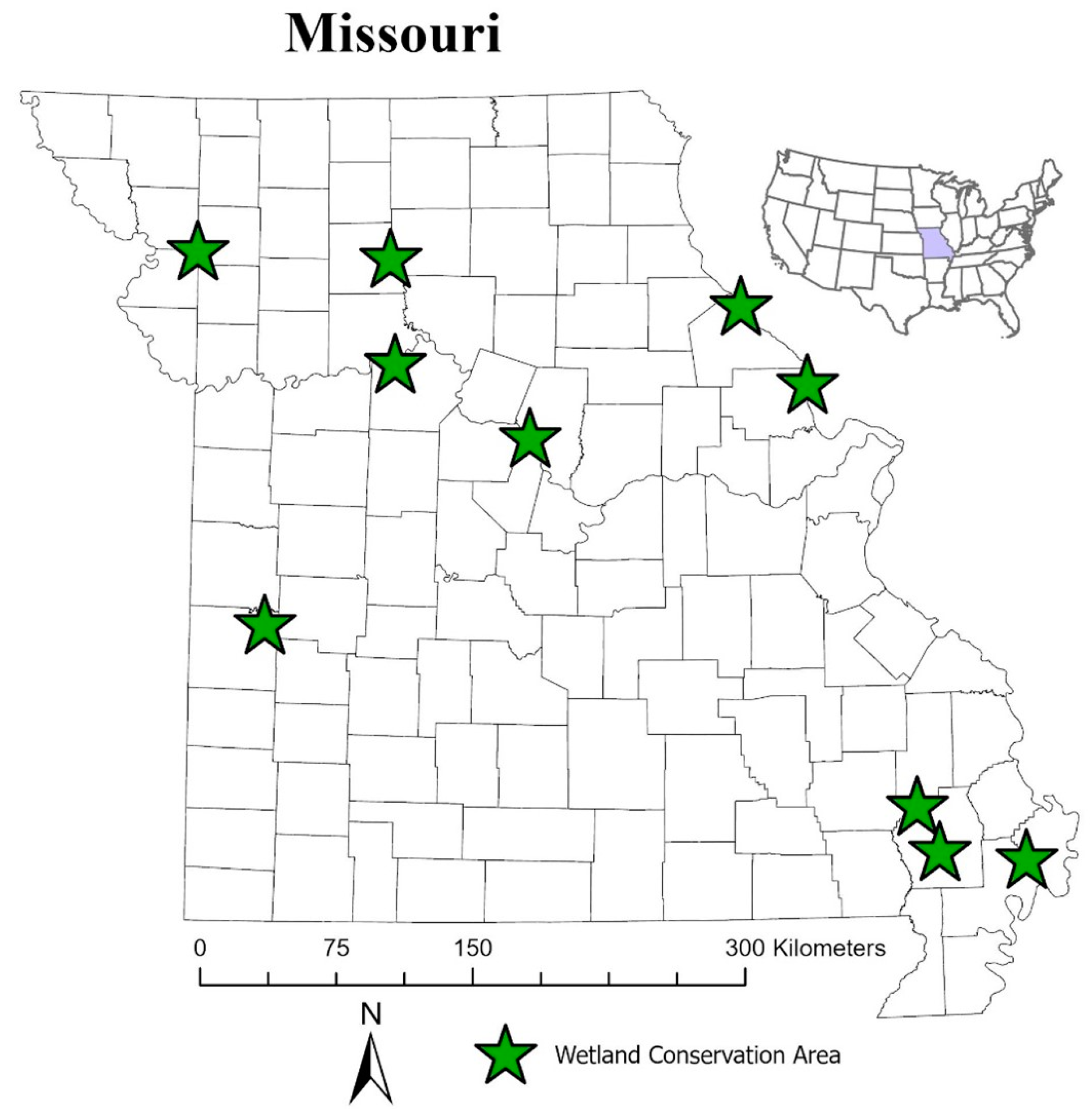
Figure 1. Intensively managed wetland conservation areas in Missouri flown by DJI Mavic Pro 2 unoccupied aerial systems over waterfowl decoys during October 2021, November 2021, and March 2022 to evaluate the availability of waterfowl and having flown over live waterfowl during October 2021/2022–March 2022/2023 to evaluate the detection probabilities of waterfowl in machine-learning-based aerial imagery surveys under different conditions.
Drones 08 00054 g001
Figure 2. Mean and 95% credible intervals of the proportion of total decoys (n = 180/image) available for detection in images taken with a DJI Mavic Pro 2 unoccupied aerial system (UAS) in Missouri, USA from October 2021, November 2021, and March 2022 dependent on ground sample distance (A), sky condition (B), and vegetation cover type (C). Ground sampling distance corresponded to flight altitudes of 15, 30, 60, and 90 m.
Drones 08 00054 g002
Figure 3. Mean and 95% credible intervals of the proportion of decoys by sex ((A), n = 90/sex/image) and species ((B), n = 30/species/image) available for detection in images taken with a DJI Mavic Pro 2 unoccupied aerial system (UAS) in Missouri, USA from October 2021, November 2021, and March 2022 across all vegetation cover types, sky conditions, and ground sampling distance (GSD). Species codes are as follows: American green-winged teal (AGWT), American wigeon (AMWI), gadwall (GADW), mallard (MALL), northern pintail (NOPI), and northern shoveler (NSHO).
Drones 08 00054 g003
Figure 4. Mean and 95% credible intervals of the proportion of birds that were correctly detected (AC) and proportion of false-positive detections generated (DF) using a deep-learning model in images taken with a DJI Mavic Pro 2 unoccupied aerial system (UAS) in Missouri, USA from October 2021–March 2022, dependent on ground sampling distance (a), sky condition (b), and vegetation cover type (c). Ground sampling distance corresponded to flight altitudes of 15, 30, and 60 m. Vegetation cover types are forested (F), harvested crop (HC), land (La), lotus (Lo), moist soil (MS), shrub–scrub (SS), and standing crop (SC).
Drones 08 00054 g004
Figure 5. Mean and 95% credible intervals of the proportion of birds that were correctly detected (A) and falsely detected (B) using a deep-learning model in images taken with a DJI Mavic Pro 2 unoccupied aerial system (UAS) in Missouri, USA from October 2021–March 2022, dependent on vegetation cover type, sky condition, and ground sampling distance. Ground sampling distance corresponded to flight altitudes of 15, 30, and 60 m.
Drones 08 00054 g005
Figure 6. Percent error of waterfowl detection algorithm counts (A) and corrected algorithm counts using a modified Horvitz–Thompson (H–T) estimator (B) compared to human labeled counts. Black line represents zero percent error, or a true (perfect) detection ratio of 1:1, with the blue line showing average trend and standard error (shading).
Drones 08 00054 g006
Figure 7. Waterfowl detection algorithm counts (A) and corrected algorithm counts using a modified Horvitz–Thompson (H–T) estimator (B) compared to human labeled counts. Black line represents zero percent error, or a true (perfect) detection ratio of 1:1, and the dashed black lines represent allowance for human labeling error of ± five percent. The blue line shows average trend and standard error (shading), with the vertical black lines showing standard error of the artificial intelligence (AI) number corrections.
Drones 08 00054 g007
Table 1. Rankings of best fitting models for predicting waterfowl decoy availability overall and by species and sex in photographs taken by a DJI Mavic 2 Pro unoccupied aerial system (UAS) at Missouri Department of Conservation intensively managed wetland Conservation Areas during October through March 2021–2022. WAIC = Watanabe–Akaike information criterion.
Dependent VariableModelCovariatesWAICΔWAIC
Overall Waterfowl AvailabilityInteraction ModelVegetation Cover Type × Sky Condition × GSD337.00.0
Additive ModelVegetation Cover Type + Sky Condition + GSD450.4113.4
Null ModelNone1937.91600.9
Species and Sex Identification AvailabilityInteraction ModelSpecies × Sex × Vegetation Cover Type × Sky Condition × GSD1502.20.0
Additive ModelSpecies + Sex + Vegetation Cover Type + Sky Condition + GSD1668.1165.9
Null ModelSpecies + Sex4380.42878.1
Vegetation cover type: The vegetation cover type in which the decoys were placed: flooded standing crop (corn [Zea mays]), moist-soil vegetation (smartweeds [Persicaria spp.], millets [Echinochloa spp. and Leptochloa spp.], and others), open water, shrub–scrub (buttonbush [Cephalanthus occidentalis], black willow [Salix nigra], and swamp privet [Foresteria acuminata]), and forested (oak species [Quercus spp.], bald cypress [Taxodium distichum], and water tupelo [Nyssa aquatica]). Sky Condition: The sky condition evident in manual review of each image: Cloudy or Sunny. Ground Sampling Distance (GSD): The image resolution (cm/pixel: 0.38, 0.76, 1.53, and 2.29), collected at four heights at which the drone was flown above the wetland: 15, 30, 60, and 90 m.
Table 2. Rankings of best fitting models for predicting the probability of a deep learning model correctly detecting (successfully detecting a visible bird) and falsely detecting (detecting something that is not a bird) waterfowl in photographs taken by a DJI Mavic 2 Pro unoccupied aerial system (UAS) at Missouri Department of Conservation intensively managed wetland Conservation Areas during November through February 2021–2022 and 2022–2023. WAIC = Watanabe–Akaike information criterion.
Dependent VariableModelCovariatesWAICΔWAIC
Probability of Correct Waterfowl DetectionsInteraction ModelVegetation Cover Type × Sky Condition × GSD4804.20.0
Additive ModelVegetation Cover Type + Sky Condition + GSD6343.91539.7
Null ModelNone7833.63029.4
Probability of False Positive Waterfowl DetectionsInteraction ModelVegetation Cover Type × Sky Condition × GSD2939.30.0
Additive ModelVegetation Cover Type + Sky Condition + GSD3765.0825.7
Null ModelNone7215.44276.1
Vegetation cover type: The vegetation cover type in which the birds were located: flooded standing crop (corn [Zea mays]), moist-soil vegetation (smartweeds [Persicaria spp.], millets [Echinochloa spp. and Leptochloa spp.], and others), open water, shrub–scrub (buttonbush [Cephalanthus occidentalis], black willow [Salix nigra], and swamp privet [Foresteria acuminata]), and forested (oak species [Quercus spp.], bald cypress [Taxodium distichum], and water tupelo [Nyssa aquatica]). Sky Condition: The sky condition evident in manual review of each image: Cloudy or Sunny. Ground Sampling Distance (GSD): The image resolution (cm/pixel: 0.38, 0.76, and 1.53), collected at three heights at which the drone was flown above the wetland: 15, 30, and 60 m.
Disclaimer/Publisher’s Note: The statements, opinions and data contained in all publications are solely those of the individual author(s) and contributor(s) and not of MDPI and/or the editor(s). MDPI and/or the editor(s) disclaim responsibility for any injury to people or property resulting from any ideas, methods, instructions or products referred to in the content.