Radiometric Improvement of Spectral Indices Using Multispectral Lightweight Sensors Onboard UAVs

Abstract

Close-range remote sensing techniques employing multispectral sensors on unoccupied aerial vehicles (UAVs) offer both advantages and drawbacks in comparison to traditional remote sensing using satellite-mounted sensors. Close-range remote sensing techniques have been increasingly used in the field of precision agriculture. Planning the flight, including optimal flight altitudes, can enhance both geometric and temporal resolution, facilitating on-demand flights and the selection of the most suitable time of day for various applications. However, the main drawbacks stem from the lower quality of the sensors being used compared to satellites. Close-range sensors can capture spectral responses of plants from multiple viewpoints, mitigating satellite remote sensing challenges, such as atmospheric interference, while intensifying issues such as bidirectional reflectance distribution function (BRDF) effects due to diverse observation angles and morphological variances associated with flight altitude. This paper introduces a methodology for achieving high-quality vegetation indices under varied observation conditions, enhancing reflectance by selectively utilizing well-geometry vegetation pixels, while considering factors such as hotspot, occultation, and BRDF effects. A non-parametric ANOVA analysis demonstrates significant statistical differences between the proposed methodology and the commercial photogrammetric software AgiSoft Metashape, in a case study of a vineyard in Fuente-Alamo (Albacete, Spain). The BRDF model is expected to substantially improve vegetation index calculations in comparison to the methodologies used in satellite remote sensing and those used in close-range remote sensing.

1. Introduction

The use of multispectral technology on board unmanned aerial vehicles (UAVs) for precision agriculture has experienced an exponential growth due to recent advances in sensor technology. These sensors have traditionally been mounted on satellite platforms and can be used for calculating vegetation indices, such as the normalized difference vegetation index (NDVI), for agricultural applications [1,2,3]. Nevertheless, UAVs offer a higher spatial resolution, temporal flexibility for image acquisition, and reduced influence of atmosphere effects (with atmosphere profiles of no more than 120 m). However, directly shifting satellite-based remote sensing methodologies to UAVs can produce radiometric differences between equivalent satellite-derived products [4,5]. Mainly, this occurs due to the presence of shadows inside the crop and because the same part of the surface is observed with different relative geometries of the two elements involved: illumination to surface and surface to sensor. Specifically, low flight height, large FoV (field of view) sensors, and the overlapping of different scenes produce a diverse observation angle for each point on the surface, and the sun’s position varies significantly throughout the flight. Another typical variation that we can expect during the flight is lighting, which depends on the time of day and the latitude. Last but not least, in the orthorectification procedure, multiple pixels from different viewing geometries are averaged together, creating overlapping images.

These properties result in the dynamism of the observed reflectance.

BRDF describes the way the surface reflects light in different directions, based on the incident angle of the incoming light and the viewing angle of the sensor; it characterizes the variability in surface reflectance due to changing geometrical conditions. As a result of the surface BRDF, the observed reflectance of a location will change based on the position of the sensor. This complicates the process of deriving reflectance values from remote sensing data and can affect the generation of vegetation indices when compared to satellite remote sensing. An example of this is found in the application of machine learning techniques to UAV-based remote sensing data processing [6,7,8,9,10]. These techniques demand multispectral or even hyperspectral bands, which require a high radiometric quality.

On the other hand, by being able to apply close-range photogrammetry techniques, an approximation of the plant envelope in 3D can be obtained, which makes it possible to determine occultations and discriminate which parts of a plant are observed in each image, with an accurate relative observation geometry with respect to both the sun and the sensor, minimizing the possible presence of shadows, which alter radiometry.

By analysing the differences in multispectral geomatic produced by UAVs, we can determine the following:

• Photogrammetric techniques pay special attention to the geometric quality of the final product [11], relegating radiometric quality. Therefore, reflectance orthomosaics, as derived from geomatic products frequently used to generate vegetation indices, can incorporate radiometric errors.
• GSD with centimetre resolution introduces BRDF effects due to the position of the sensor and changes in illumination angles during the flight. The pixel size of most satellite images exceeds one metre and is usually several orders of magnitude coarser in resolution compared to that of a UAV image.

Specifically, the pixel of a remote sensing product from public space missions has a spatial resolution of several meters (Sentinel-2A/2B has a 10 m–60 m spatial resolution in both the visible and the NIR bands, while Landsat-8/9 imagery has both a 15 m panchromatic and a 30 m multi-spectral spatial resolution), and the collected data are the aggregation of the plant canopy and soil. In contrast, UAVs can achieve spatial resolutions even higher than 0.05 m. The high spatial resolution, together with the large number of points of view from which the canopy is acquired when using UAVs, leads us to consider the convenience of choosing image pixels from the plant that are better aligned with a geometry of choice (e.g., a satellite sensor or a consistent geometry for temporal studies), involving making decisions such as:

• Only using data from the canopy (not from the ground or trunk/branch) using spatial and radiometric criteria, discriminated by height from the DSM with DTM as a reference [12], and approximating NDVI using the classical method [13].
• Ignoring parts of the crop that are hidden in an image due to the geometry of the crop (obtained from a DSM generated as a satellite photogrammetric product) and image orientation.
• Avoiding image areas that may be affected by the hotspot effect [14] and correcting the images by using the directional property of reflectance.
• Only using image pixels acquired from a favourable geometry or optimal perspective with respect to the canopy and the sun position, discriminated using the image orientation and the sun position at the time of image acquisition.

The BRDF effect is a classic issue in remote sensing and its correction has given rise to different modelling proposals that are not usually included in the standard process for generating products prepared for ARD analysis (analysis ready data) due to its practical difficulty [15]. The hotspot effect is also a classic drawback in remote sensing and its correction is included in some BRDF models. A hotspot is a circular bright area within the image that is produced due to a direct alignment between the sun, the camera, and the position on the ground [14]. In other words, it is placed at the projected solar position, opposite the specular reflection position. The probability of a hotspot effect is also increased in UAV flights due to the wide angle of view of the optics and the interest in flying over plant covers at times when the sun is higher over the horizon because of shadow reduction and an increase in photosynthetic activity. Moreover, the effect of shady areas on the canopy is also corrected in some BRDF models.

There are BRDF models that can be applied to near-range remote sensing from UAVs, so called Kernel-driven models, such as the empirical Walthall model and the non-linear RPV model [16], which improve ARD products by correcting the reflectance in each band. In the last two years, several articles have been published addressing the BRDF effect from UAV imagery [17,18]. However, they do not rigorously consider the mathematical model of photogrammetry, the concealment effects based on the knowledge of the canopy geometry through the DSM, the elimination of areas in the images affected by the hotspot effect, and the consideration of optimal perspectives for removing the leaf pixels in which the vegetation cover is not directly exposed by the sun.

Given the relevance of these issues, this study focuses on addressing a radiometric improvement of multispectral data captured through UAV platforms. In this context, this paper presents a comparative analysis of the red (R), green (G), blue (B), red edge (RE), and near infrared (NIR) reflectance bands, as well as the NDVI index, obtained through two different approaches:

• Utilizing the conventional photogrammetric computer tool AgiSoft Metashape.
• Implementing a novel methodology that addresses the aforementioned problems.

  -

  Introducing corrections for the BDRF effect per ortho-image by precisely computing the external orientation of the images and the relative orientation of the object to the acquisition point and to the sun.

  -

  Using the information derived from individual ortho-images rather than geomatic products obtained through photogrammetric processes, while eliminating the radiometric distortion that these processes may incorporate.

  -

  Determining the optimal pixel values from the best ortho-image considering factors such as lighting, possible occultations, and the relative position within the image.

This paper employs a comparative analysis of variance (ANOVA) in order to evaluate the differences and advantages provided by the proposed methodology in comparison to conventional methods for the acquisition and processing of radiometric data. ANOVA is a robust statistical methodology to assess variances in datasets, discern the disparities between group means, and explore the sources of variability [19]. This technique quantifies the variation within and between groups to infer whether observed differences are attributable to random chance or systematic effects. Many articles on the use of ANOVA analysis in agronomy can be found in the literature [20,21,22,23].

2. Materials and Methods

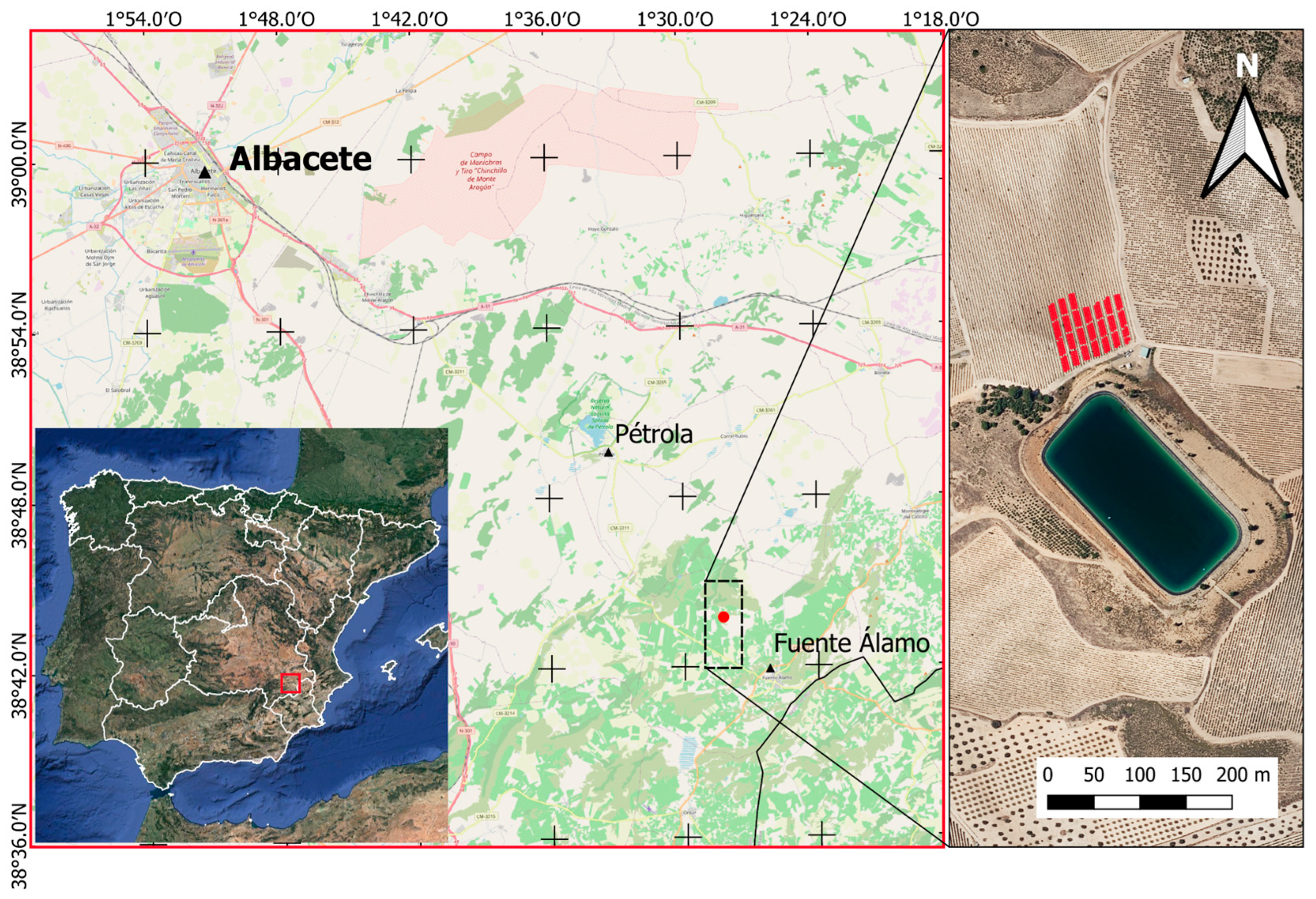
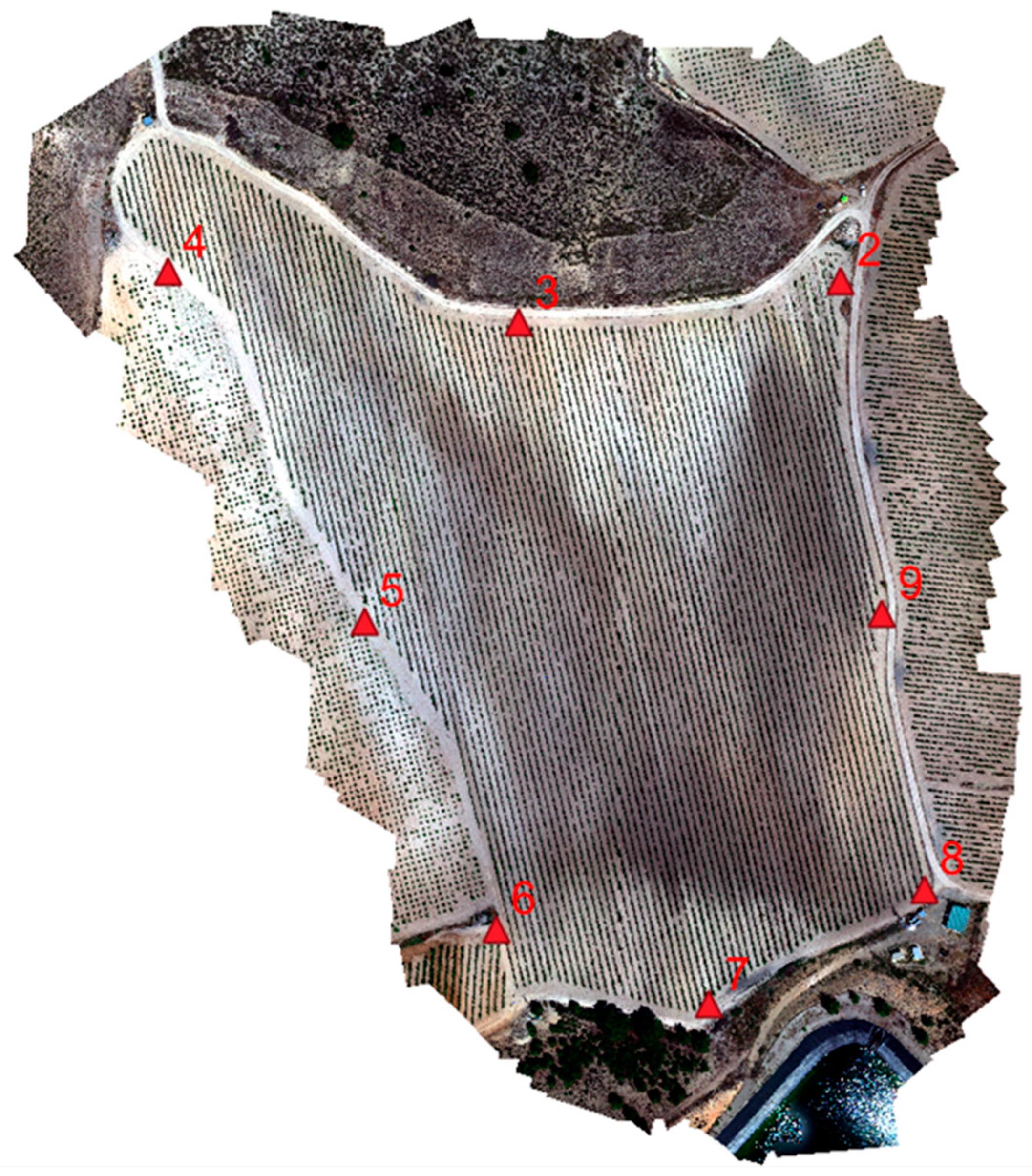
2.1. Experimental Setup

The field experiment was conducted in a commercial vineyard located in Fuente-Alamo, Albacete, Spain (38.43043300 N, 1.28012600 W; elevation 820 m above sea level) during the 2020 growing season (Figure 1). The climate is defined as typical Mediterranean semiarid [24], with hot and dry summers and daily maximum summer temperatures close to 40 °C, mainly in July and August. The trial was carried out in a 0.6-hectare subplot of a 6.5-hectare commercial vineyard. The soil was sandy loam (with more than 55% sand), with a variable depth of up to 90 cm. The soil had 1.2% organic matter, 47.7% active CaCO₃, an electrical conductivity of 0.4 dS/m, a pH of 8.9, and a bulk density of 1.2 g/cm³. The vineyard rows were oriented north–south. The inter-row was regularly tilled and the soil under the vine rows was kept weed-free through the use of herbicides.

2.2. Data Acquisition

The photogrammetric sensor used is a MicaSense RedEdge^® camera (MicaSense Inc., Seattle, WA, USA [25]). It is one of the most efficient low-cost multispectral sensors onboard a UAV. It is formed of five dedicated sensors with a narrow-band filters for detecting data, respectively, in the B, G, R, RE, and NIR wavelengths. It has a global shutter to avoid problems in data processing regarding dark current and UAV movements during the flight [26]. The camera specifications are detailed in

Table 1. Technical specifications of the MicaSense RedEdge sensor (MicaSense Inc., Seattle, WA, USA).

Weight	170 g (including DSL)
Dimensions	9.4 cm × 6.3 cm × 4.6 cm
External power	4.2 V–15.8 V, 4 W nominal, 8 W peak
GSD	8.2 cm/pixel at 120 m AGL
Blue spectral band	Centre wavelength: 475 nm Bandwidth FWHM: 20 nm
Green spectral band	centre wavelength: 560 nm Bandwidth FWHM: 20 nm
Red spectral band	Centre wavelength: 668 nm Bandwidth FWHM: 10 nm
Red edge spectral band	centre wavelength: 717 nm Bandwidth FWHM: 10 nm
NIR spectral band	Centre wavelength: 840 nm Bandwidth FWHM: 40 nm

, where FWHM is the full width at half maximum. The MicaSense RedEdge camera works with the downwelling light sensor (DLS), using the same spectral bands, which are cosine-corrected light sensors that help improve the radiometric quality of the image data by providing a direct way of measuring reflectance without using a reference target. Light sensors are the most effective at correcting for global changes in lighting conditions.

The resolution of the photogrammetric sensor was 1280 × 960, with a pixel size of 3.75 × 3.75 µm. The focal length was fixed at 5.5 mm. The total coverage area was 0.14 km². The sensor was mounted on a quadcopter Carabo S3 (Icom3D, Asturias, Spain) (Figure 2). The flight planning was performed by using UAV-GeoFlip Geomatic Flight Planning software [27]. The flight was planned and executed to establish a minimum forward overlap of 60% and a minimum side overlap of 20%, with a GSD of 5.09 cm/pix for the DSM (digital surface model). The flight was performed near solar noon (between 11:00 and 12:00 solar time) to reduce the grapevine shadow on the images, with an altitude of 80 m to reach the required GSD. A total of 8 GCPs (ground control points) were located (Figure 3) to be easily detected from the UAV images and topographically measured via GNSS-RTK for georeferencing. The locations and georeferenced errors are indicated in

Table 2. Locations and geo-referencing errors of the GCPs.

Markers	Easting (m)	Northing (m)	Altitude (m)	Error (m)
2	632,939.341	4,288,036.966	830.224	0.0046
3	632,805.756	4,288,019.635	830.205	0.0064
4	632,659.743	4,288,040.656	835.192	0.0007
5	632,741.361	4,287,895.546	825.769	0.0083
6	632,796.057	4,287,767.781	822.259	0.0195
7	632,884.765	4,287,736.708	821.987	0.0173
8	632,973.799	4,287,784.585	818.104	0.0034
9	632,956.238	4,287,898.923	823.163	0.0068

. In addition, 4 reflectance panels were placed in the study field, and they were captured at the beginning and at the end of the flight for radiometric calibration purposes. The flight was performed during clear sky conditions. Finally, a total of 2685 images were acquired (537 images per band) by the MicaSense RedEdge^® camera.

2.3. Reference Commercial Multispectral Software (AgiSoft Metashape)

A standard photogrammetric pipeline was used to process the multispectral UAV imagery, applying camera calibration, image orientation and a dense point cloud extraction process. The AgiSoft Metashape software package (AgiSoft LLC, St. Petersburg, Russia [11]) was used for that purpose. As an alignment parameter, a limit of 4000 tie points was used. Moreover, 8 GCP measurements were utilized for recovering the camera’s interior parameters and correcting for any block deformation or systematic error to be able to absolutely geo-reference and geometrically calibrate the images. The geo-referencing RMSE of the GCPs was 1.04 cm. The overall reprojection error was 0.44 pixels, based on the bundle-adjustment error assessment report. The tie point projection errors were considered to eliminate poor-quality points. Moreover, a noise filter was applied during the point cloud generation to improve the quality of the ortho-mosaic. An aggressive filtering was used to preserve as much detail as possible over the canopy structure. Finally, the DSM and the ortho-mosaic were created by ortho-rectifying the image pixels with a 6 cm GSD. In order to simulate the radiant attenuation for vignetting correction, a distance to the surface model was performed per pixel. Moreover, the DTM resolution was 20.3 cm/pix (DSM GSD fitting to the ground) and the compound coordinate reference system was ETRS89/UTM zone 30N (EPSG 25830, 5782). Orthometric heights refer to the tide gauge in Alicante. Reflectance ortho-mosaics were computed using the internal calibration of AgiSoft Metashape software, with the calibration panel pictures and the DLS [28].

2.4. BRDF Correction

The proposed procedure aims to calculate the best possible reflectance value per band. A classical property to consider when disturbing image radiometry is the bidirectional reflectance from the ground surface (BRDF). The most prominent issue in aerial images occurs at high solar elevation, where the hotspot can occur. The Walthall model [29] describes the directional reflectance of visible and NIR radiation as a function of zenith and azimuth view angles and solar azimuth angle for several canopies and bare soil surfaces. The access to the directional domain allows normalizing the anisotropy or incorporating the directional signature as a source of additional information.

The Walthall model [29] is a simple linear empirical model, working under clear sky conditions. It uses a three-term parametrization (p₀, p₁, p₂), following Equation (1):

$$R^W \left({\theta }_v,\varphi ;\lambda \right)=p_0\left(\lambda \right){\theta }_v^2+p_1\left(\lambda \right){\theta }_v\cos \varphi +p_2\left(\lambda \right)$$

(1)

where R^W is the observed surface reflectance in each band, W, measured by the camera after calibration with standard panels and the downwelling light sensor (DLS) under ${\theta }_v$ as an observation zenith angle, with a relative azimuth angle $\varphi$, and wavelength $\lambda$; p₀, p₁ and p₂ are constants; $p_0\left(\lambda \right){\theta }_v^2$ and $p_1\left(\lambda \right){\theta }_v\cos \varphi$ are terms that have to be eliminated so that there is no BRDF effect; $p_2\left(\lambda \right)$ is reflectance at nadir view and illumination.

The rigorous photogrammetric model provided allows the ability to compute for each pixel the angles of the equation, and p₀, p₁, and p₂ can be estimated by least squares adjustment. The ${\theta }_v^2$ term describes the concave shape of the BRDF associated with the gap effect. The term ${\theta }_v\cos \varphi$ term provides a linear dependency between reflectance and the ${\theta }_v$ angle, describing the BRDF anisotropy and the increase in reflectance due to backscatter. This second term, therefore, basically collects the back-shadow effect.

The Walthall model is one of the most robust models at different scales on a wide variety of surfaces [30]. However, this model does not reproduce the reciprocity principle.

The steps to apply the proposed methodology are described below (Figure 4).

The final outcome of this methodology provides crop-optimised reflectivities using all pixels of all images, but these results are not satisfactory for the different criteria considered. From these corrected reflectivities, any index could be calculated, with NDVI being the index computed for this paper because it is one of the most widely used in precision agriculture applications.

2.4.1. Pre-Processing

First, a photogrammetry project in QGIS should be created, and the data imported. Pre-processing inputs are automatically obtained with a reference software from structure from motion (SfM), AgiSoft Metashape Professional Edition photogrammetry software (already explained in Section 2.3). With this step, the entire mathematical model is already set up. It consists of creating the database, assigning the CRS (coordinate reference system), importing the markers.xml file from the project (which includes camera calibration and image orientations), and importing the path to the project’s raw images. Later on, the EXIF information of the raw images is obtained. It includes the acquisition time to calculate the sun data (i.e., solar angles) and parameters for the reflectance conversion model, according to the MicaSense manual.

After that, the DSM and DTM are produced with AgiSoft Metashape Professional Edition photogrammetry software (already explained in Section 2.3). Plant angles, heights, and hidden parts are automatically defined. This step allows us to compute the image footprints on the DSM to get the framework for the orthoimages.

2.4.2. Radiometric Processing

For each image, the sun position (zenith and azimuth) and hotspots are computed, following the methodology published by [14]. The instant of observation is considered as a variable that comes from the EXIF. The hotspot effect is produced due to a direct alignment between the sun, the camera, and the position on the ground; that is, the point on the ground opposite the sun in relation to the camera. The hotspot produces a change of brightness in this point of the image and its surroundings. These regions will be excluded in the last step, in which the reflectivity statistics by band and plant are calculated.

Next, the digital numbers (DNs) are converted to reflectances. For this case, the mathematical model used can be found in MicaSense Image Processing Tutorials [31]. The software computes the radiometric corrections using the white reference panel and the irradiance sensor (DLS). Three different options have been contemplated: using only one or several measurements, with temporal interpolation, or with the closest value in time. This can be achieved by using camera calibration parameters (such as AgiSoft Metashape software), using only DLS information, or adopting a mixed solution that combines calibration parameters and DLS data (which is the one used for the current work).

If the panel is used, the calibration process can be computed at the beginning of the flight or, if the panel is captured at the beginning and the end of the flight, the calibration process interpolates the correction for each image capture event. To obtain reflectance images, first, the conversion factors per band from the panel images are retrieved. For this, panel coordinates from GPS EXIF together with solar zenith and azimuths are computed. The conversion factors are retrieved (gain and offset) from the mean digital value of the panel, corrected for vignetting.

However, if DLS information is employed, conversion factors are retrieved from the MicaSense model through solar position, horizontal irradiance, and direct or diffuse radiation data (depending on the sensor). In both pipelines, reflectance images are computed using the conversion factor, interpolating as a function of time. After this, the orthoimages are computed per band with a GSD similar to the DSM exported from Metashape. The hidden pixels calculated from the DSM are left without data because, in the projective ray in which they are included, there is another point from the DSM which is closer to the optical centre. Moreover, raster files are saved with distances and angles (zenith and azimuth) from each pixel projected on the plant to the projection centre of the camera position with centimetre accuracy. Lastly, NDVI ortho-images are generated per band.

2.4.3. Optimized Reflectances from the BRDF Correction Model and Derived NDVI

For each plant, we start from the planimetric definition of the planting frame. Thereby, for each DSM pixel above the DTM at a height higher than the established threshold (0.2 m in this case), an algorithm is used to obtain the optimized reflectance per band. To achieve this, a sample of reflectances and auxiliary values for the BRDF model (azimuth and elevation of the sun and sensor) are computed. To obtain this sample, image pixels that do not meet at least one of the following filter criteria are eliminated:

• Is in a hotspot zone.
• Is hidden using the DSM.
• The normalized difference vegetation Index (NDVI) in the orthoimage from the previous step is outside the chosen range (between 0.2 and 1.0 in this case). Consequently, the vegetation is segmented by the NDVI filter calculated with 3-decimal places.
• The horizontal angle between the plant formed by the direction between the sun and the sensor is outside the established range (from −90 to 90 degrees in this case).

With these samples, the BRDF model is adjusted to obtain corrected reflectances. The reflectance per plant is computed using a multi-view statistical analysis. It involves an iterative least squares (LS) solution with an observation removal process, guided by a threshold in the residuals. Moreover, the adjusted reflectance solution is considered valid based on the standard deviation using a generalized method of moments (GMM) and statistical limits. The reflectance of those plants with insufficient information is avoided. The NDVI is obtained from the optimized reflectances.

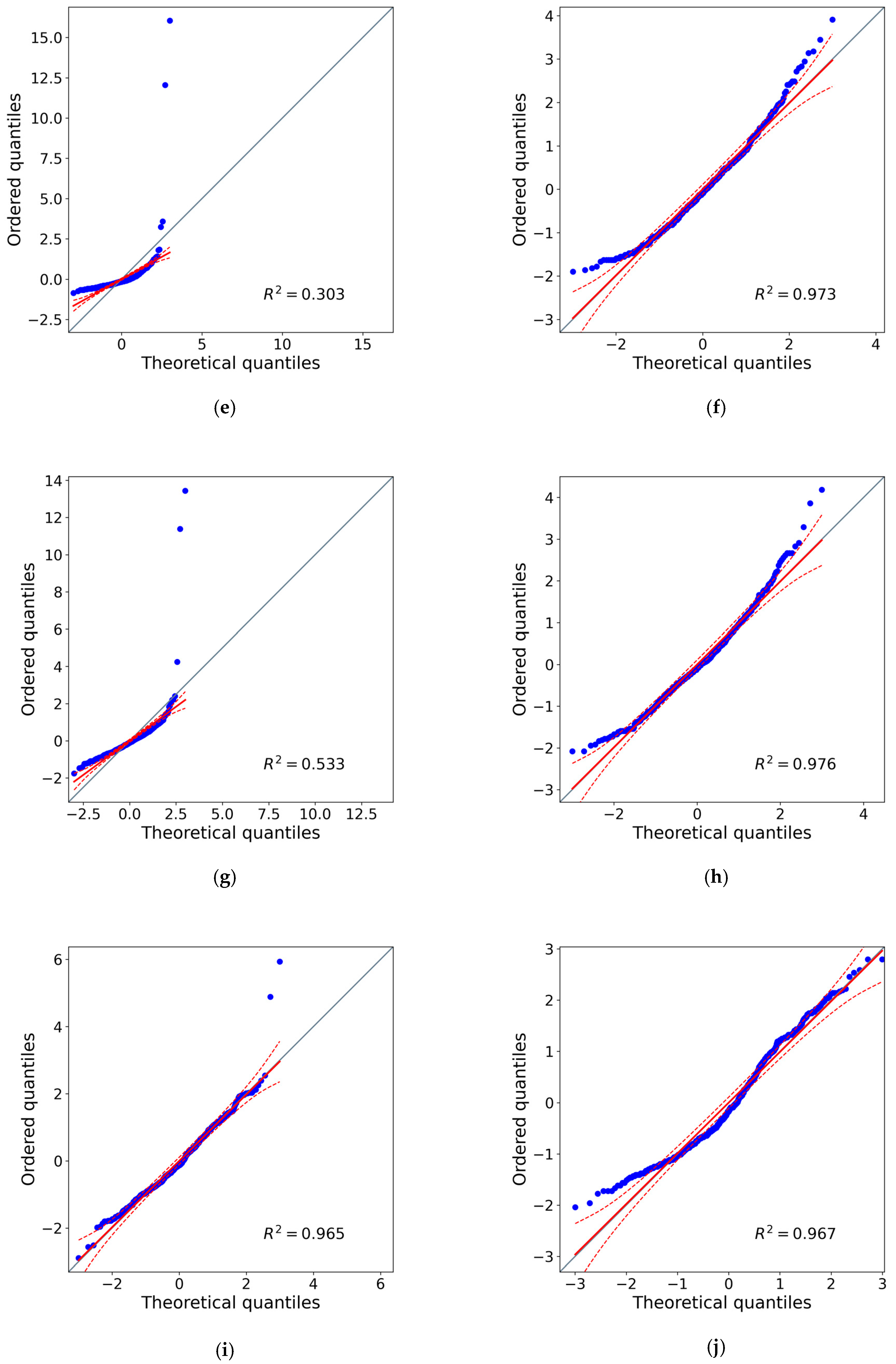
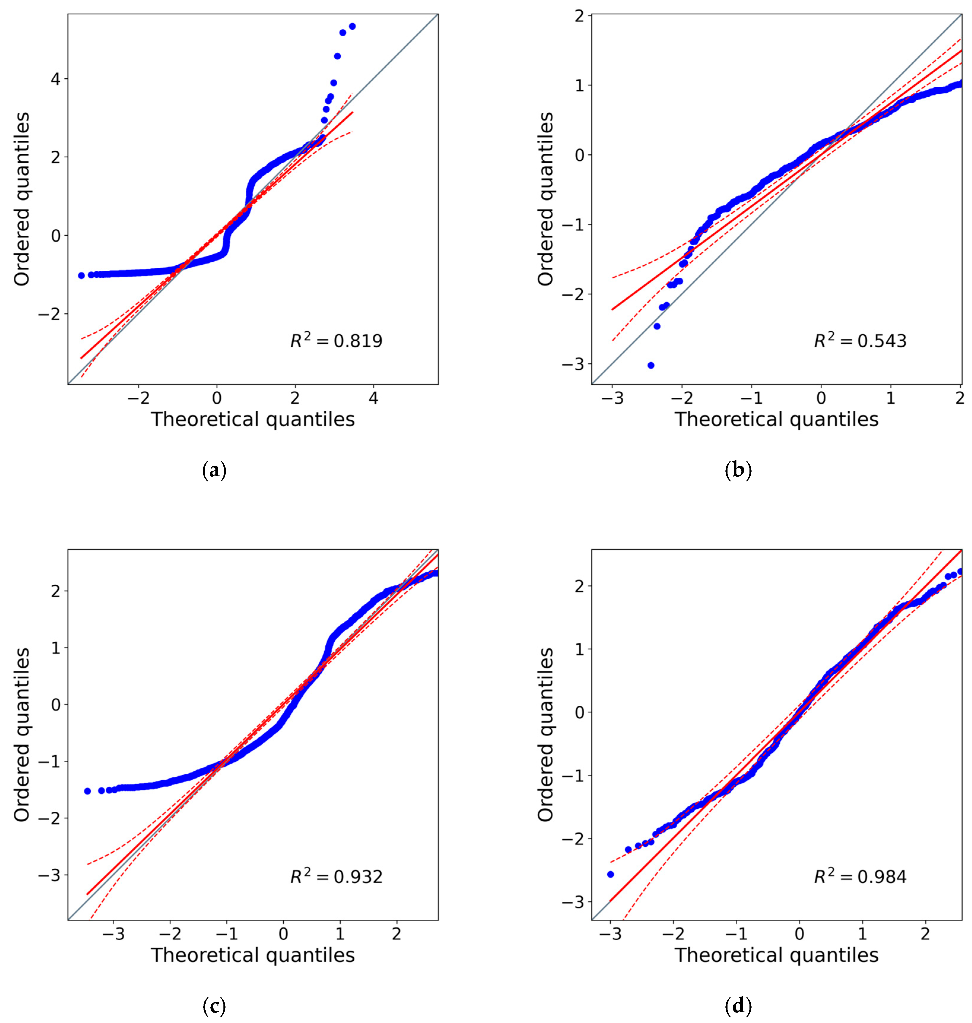
2.5. Statistical Analysis

In this study, two datasets obtained using different methodologies are available. On the one hand, we have the reflectance data obtained by applying the BRDF correction, as explained in the previous sections, and the reflectance data provided by the commercial software Metashape. For simplicity, we will refer to these methods as M_BRDF and Metashape, respectively. The NDVI values, calculated from the R and NIR bands, are available for both methods. In order to identify statistically significant differences between the M_BRDF and Metashape methodologies, an ANOVA, or analysis of variance test, was used. Figure 5 shows schematically the workflow carried out for the ANOVA analysis, which we explain in detail below.

In a nutshell, ANOVA splits the total variance in the data into two components: variance between groups and variance within groups. The ratio of these variances is used to calculate an F-statistic, which, when compared to a critical value, helps to determine the statistical significance of group differences. The null hypothesis establishes that there is no significant difference between the group means. If the p-value is less than the critical value (usually 0.05), the null hypothesis is rejected and it can be concluded that there is a significant difference between the means [32,33].

Predominantly, ANOVA can be applied following three different approaches: one-way ANOVA, two-way ANOVA, and factorial ANOVA. The one-way ANOVA methodology finds its utility when there exists a sole categorical independent variable, while two-way ANOVA extends its purview to encompass the dynamics of two independent variables. The third approach is achieved through factorial ANOVA, which permits the meticulous scrutiny of multiple independent variables and their mutual interactions.

On the other hand, ANOVA can be approached from both parametric and non-parametric perspectives. Parametric ANOVA assumes that the data follow a normal distribution and that the variances between groups are approximately equal (i.e., homoscedasticity). If the data deviate from these assumptions, non-parametric ANOVA can be used. A normality test, such as the Shapiro–Wilk test, will determine which type of ANOVA is required. In addition, a prior analytical and graphical study of the data is often helpful for understanding the nature of the data.

The parametric approach uses the F-statistic to assess the presence of significant variance differences between groups, while the Mann–Whitney U test serves for assessing the presence of statistically significant differences between two independent groups in those cases where the data deviate from the assumptions of normal distribution and equality of variances. This non-parametric test involves ranking the data, calculating separate U statistics for each group, and determining the minimum U statistic as the critical value. Thus, through hypothesis testing, the Mann–Whitney U test evaluates whether this test statistic significantly differs from what would be expected by chance [34,35].

Various non-parametric tests can be used to statistically compare more than two independent data sets. Taking into account the nature of our data, the most appropriate non-parametric test is the Kruskal–Wallis H test. It is actually an extension of the Mann–Whitney U test, which is used to compare two independent groups. The Kruskal–Wallis H test is particularly useful when the data do not meet the assumptions of parametric tests [36,37]. However, it is common to encounter outliers when applying this type of statistical test. To this end, an additional check based on the Yuen t-test can be applied to the reflectance and NDVI data, since this test is more robust against the presence of outliers [38,39].

The drawback of ANOVA is that although the results obtained show that there are significant differences between groups, the test itself does not specify which groups exhibit these differences. In this sense, post hoc tests, such as the Bonferroni test, help to identify pairwise differences among groups, providing a more detailed and actionable understanding of the data [40]. Therefore, it is advisable to perform the post hoc analysis when the ANOVA results are significant.

3. Experimental Results

As stated in the statistical analysis subsection, it is necessary to study the data beforehand, as the ANOVA to be applied will depend on the nature of the data.

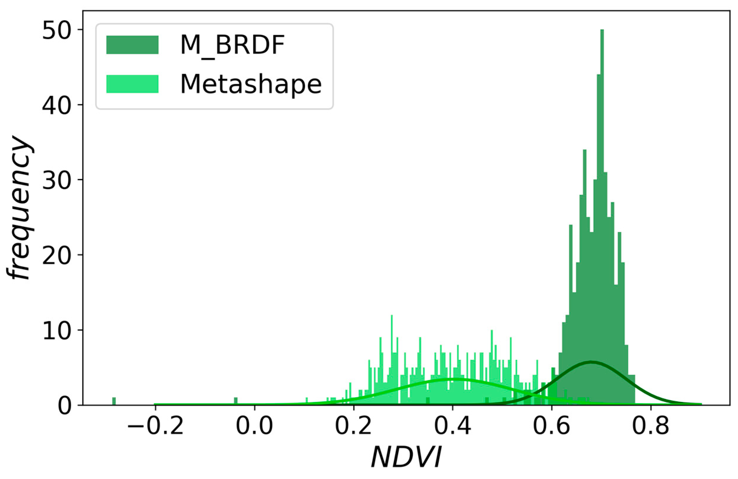
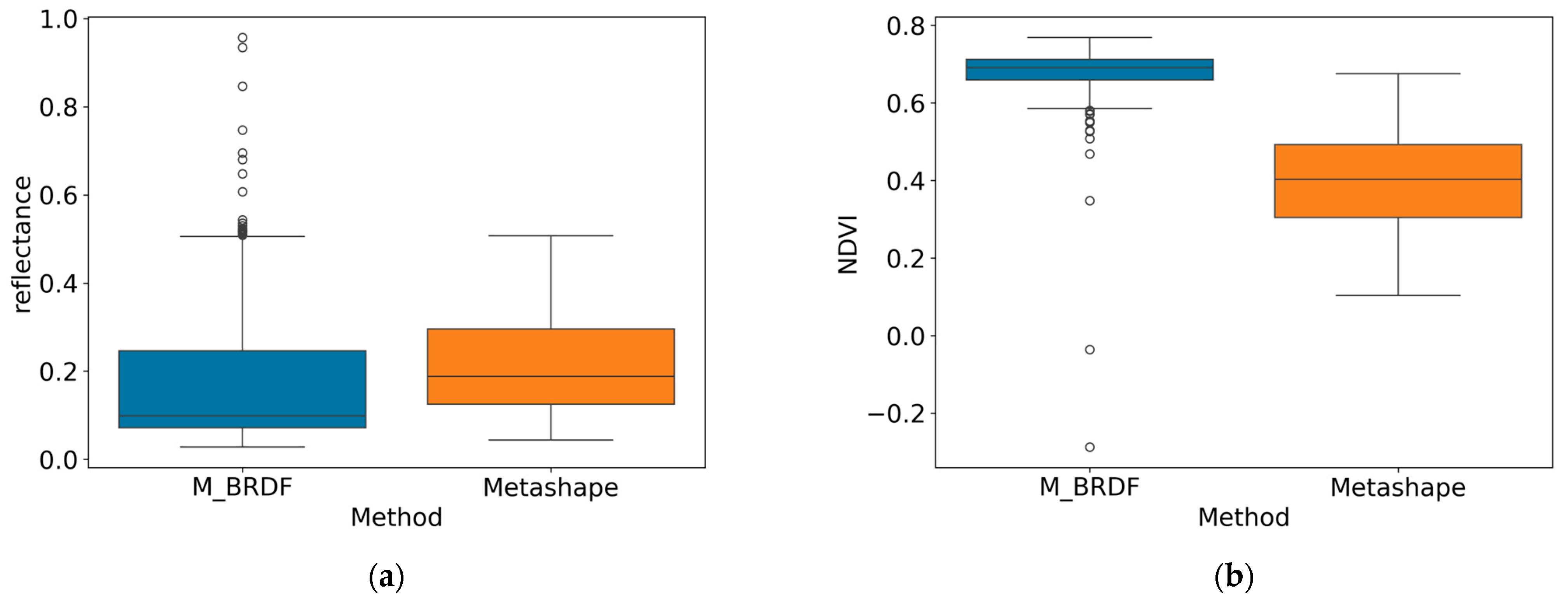
3.1. Reflectance Analysis per Band and NDVI

Three assumptions must be met in order to use a parametric ANOVA; that is, independence of de data, assumption of normality, and homogeneity of variance (i.e., homoscedasticity). The independence condition is fulfilled, since the methodologies used to obtain the reflectance are independent. Therefore, a normality test must be applied to the data, which will determine whether a parametric or non-parametric ANOVA should be used since it is a critical condition of the ANOVA test.

However, it is useful to carry out a prior graphical and analytical study of the main statistics of the data.

Table 3. Reflectance statistics for each method and band.

	M_BRDF					Metashape
	R	G	B	RE	NIR	R	G	B	RE	NIR
Mean	0.084	0.099	0.051	0.230	0.429	0.174	0.152	0.093	0.273	0.401
Std.	0.050	0.038	0.026	0.054	0.045	0.049	0.033	0.026	0.037	0.038
Min.	0.055	0.060	0.028	0.135	0.299	0.074	0.085	0.044	0.196	0.323
25%	0.071	0.087	0.042	0.205	0.397	0.136	0.129	0.073	0.248	0.370
50%	0.079	0.095	0.047	0.225	0.423	0.172	0.149	0.091	0.270	0.394
75%	0.087	0.105	0.053	0.246	0.459	0.206	0.169	0.109	0.293	0.431
Max.	0.934	0.680	0.473	0.957	0.695	0.389	0.296	0.195	0.427	0.507

shows the main statistics, taking into account the reflectances obtained for each of the bands (R, red; G, green; B, blue; RE, red edge; NIR, near infrared), according to the method used. Figure 6 shows the histogram for each band, separated by method. The theoretical normal distribution is also included with the histogram plot. On the other hand,

Table 4. NDVI statistics for each method.

	M_BRDF	Metashape
Mean	0.680	0.403
Std.	0.070	0.117
Min.	−0.287	0.104
25%	0.659	0.304
50%	0.691	0.403
75%	0.712	0.493
Max.	0.769	0.675

. shows the statistics for the NDVI values calculated for both methods, while Figure 7 shows their histogram, including the theoretical normal distribution.

The preliminary analysis of the data, particularly the histograms, shows evidence of non-normality, especially in the reflectance (Figure 6) and NDVI values obtained by applying the M_BRDF correction (Figure 7). Although at first sight, the data obtained using Metashape software seem to fit the normal distribution better, it is interesting to note that they tend to be more homogeneous than those obtained using the M_BRDF correction (Figure 6a vs. Figure 6b). This homogeneity is related to the methodology used in Metashape itself, which will be discussed later, in Section 4. On the other hand, the data obtained via M_BRDF, especially the NDVI, provide more adjusted reflectance values and a greater diversity and range due to the complex corrections taken into account in the methodology. Thus, it is also clear that the data obtained using the two methods are statistically different, as shown by their means and standard deviations (Table 3 and Table 4). This intuitive conclusion will be confirmed by the application of the ANOVA test.

After the preliminary graphical analysis, we apply the Shapiro–Wilk normality test to the data.

Table 5. Shapiro–Wilk normality test results.

Method	Data	Statistic W	p-Value
M_BRDF	Reflectance	0.818758	0.0
	NDVI	0.552042	5.717402 × 10−34
Metashape	Reflectance	0.931502	1.305781 × 10−32
	NDVI	0.98261	0.000009

shows the results for the W statistic and the p-value obtained. In addition, Figure 8 shows the graphical QQ plots for visual inspection. Further details of the results of the normality tests applied per method and band are given in

Table A1. Shapiro–Wilk normality test results specified by method and reflectance band.

Method	Band	Statistic W	p-Value
M_BRDF	R	0.208354	1.289054 × 10−41
	G	0.316521	1.448288 × 10−39
	B	0.311016	1.122708 × 10−39
	RE	0.541758	2.936743 × 10−34
	NIR	0.968362	5.374462 × 10−9
Metashape	R	0.979078	0.000001
	G	0.970273	1.283545 × 10−8
	B	0.972804	4.288144 × 10−8
	RE	0.97577	1.919421 × 10−7
	NIR	0.965455	1.515331 × 10−9

, together with the corresponding QQ plots in Figure A1 in Appendix A.

The p-values obtained are all less than 0.05, so the null hypothesis is rejected, confirming that the data deviate from the normal distribution (Table 5). The same conclusion can be reached by looking closely at the QQ plots (Figure 8). Since the results show clear evidence that the data deviate from the normal distribution, a non-parametric ANOVA test should be applied.

Once it is confirmed that the assumption of normality of the data is not met, the non-parametric statistical tests described in Section 2.5 are applied to perform the ANOVA analysis (i.e., the Mann–Whitney U test, the Kruskal–Wallis H test, and the Yuen t-test). The results obtained for these tests are shown in

Table 6. Non-parametric ANOVA statistical tests.

Test	Data	Statistic	p-Value
Mann–Whitney U test	Reflectances	2,254,515.5	0.000
	NDVI	253,900.0	0.000
Kruskal–Wallis H test	Reflectances	338.385	0.000
	Band	4637.855	0.000
	NDVI	722.978	0.000
Yuen t-test	Reflectances	2291.348	0.000
	NDVI	41.920	1.6245 × 10−181

.

Since the p-values obtained for the U-test are less than 0.05, the null hypothesis is rejected, so we can state that there are significant differences between the means of the groups compared, i.e., between the reflectance and NDVI data obtained via the M_BRDF and Metashape methods (Table 6). This difference between the groups can be clearly seen in Figure 9, where the box plots for reflectance and NDVI are shown. Furthermore, the same conclusion can be reached by analysing the p-values obtained via the H-test for the same datasets, since they are lower than the critical value of 0.05, thus rejecting the null hypothesis.

It is interesting to note, however, that the H-test shows that there are also significant differences when comparing reflectance data by spectral band. Again, these differences can be clearly seen in Figure 10, where the box plot is shown, taking into account the spectral bands for both methods.

Finally, since the non-parametric ANOVA results obtained are significant, a Bonferroni post hoc test was applied in order to determine which specific bands differed significantly. The results show p-values equal to 0 for all possible band combinations, confirming that each of the bands is significantly different for both methodologies. Further details are given in

Table A2. Bonferroni post hoc statistical results.

A	B	U-Value	p-Value
M1.1 1	M12	50,988.500	0.000
M1.1	M13	246,558.000	0.000
M1.1	M14	1060.500	0.000
M1.1	M15	1014.000	0.000
M1.1	M21	5304.500	0.000
M1.1	M22	5050.000	0.000
M1.1	M23	89,305.000	0.000
M1.1	M24	1014.000	0.000
M1.1	M25	1014.000	0.000
M1.2	M1	3,253,265.500	0.000
M1.2	M14	1513.000	0.000
M1.2	M15	1011.000	0.000
M1.2	M21	14,433.000	0.000
M1.2	M22	14,414.500	0.000
M1.2	M23	144,301.000	0.032
M1.2	M24	1103.500	0.000
M1.2	M25	1014.000	0.000
M1.3	M14	1011.000	0.000
M1.3	M15	456.500	0.000
M1.3	M21	1377.000	0.000
M1.3	M22	1439.000	0.000
M1.3	M23	11197.500	0.000
M1.3	M24	1005.000	0.000
M1.3	M25	602.500	0.000
M1.4	M15	1459.000	0.000
M1.4	M21	212,272.000	0.000
M1.4	M22	243,981.000	0.000
M1.4	M23	256,848.500	0.000
M1.4	M24	43,776.500	0.000
M1.4	M25	1624.000	0.000
M1.5	M21	256,930.000	0.000
M1.5	M22	257,049.000	0.000
M1.5	M23	257,049.000	0.000
M15	M24	255,821.000	0.000
M15	M25	176,590.000	0.000
M21	M22	163,985.000	0.000
M21	M23	240,322.500	0.000
M21	M24	13,782.000	0.000
M21	M25	304.000	0.000
M22	M23	237,125.000	0.000
M22	M24	2411.500	0.000
M22	M25	0.000	0.000
M23	M24	0.000	0.000
M23	M25	0.000	0.000
M24	M25	2506.500	0.000

¹ M1 = M_BRDF; M2 = Metashape; 1 = R; 2 = G; 3 = B; 4 = RE; 5 = NIR.

in Appendix A.

It should be noted that the non-parametric ANOVA analysis for this study was carried out using a proprietary script programmed in Python. Both the study data and the code are published on GitHub [41].

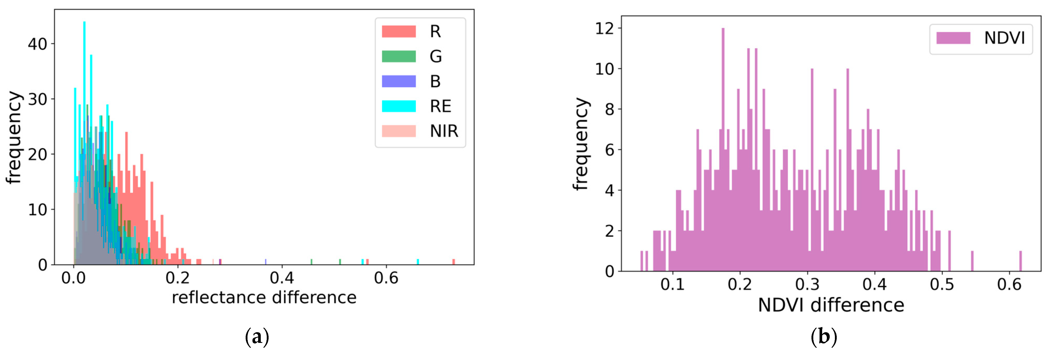
3.2. Spectral Band and NDVI Differences

The non-parametric ANOVA established a statistically significant distinction between the M_BRDF and Metashape methods. In this section, we undertake a comprehensive examination of the disparities in reflectance and normalized difference vegetation index (NDVI), with a specific emphasis on their absolute magnitudes, irrespective of the sign of the differences. Our analysis combines both analytical and graphical approaches.

Table 7. Reflectance band and NDVI absolute differences for each method.

	∆R	∆G	∆B	∆RE	∆NIR	∆NDVI
Mean	0.095	0.057	0.045	0.050	0.034	0.281
Std.	0.058	0.041	0.031	0.049	0.027	0.109
Min.	0.002	0.001	0.005	0.001	0.000	0.052
25%	0.055	0.030	0.024	0.022	0.017	0.193
50%	0.089	0.053	0.041	0.043	0.029	0.270
75%	0.125	0.073	0.061	0.067	0.045	0.375
Max.	0.732	0.513	0.370	0.663	0.284	0.619

provides essential statistical metrics characterizing the absolute differences in reflectance, with consideration given to the spectral bands. Additionally, the absolute NDVI differences originating from both datasets are detailed. Furthermore, Figure 11 visually depicts the distribution of absolute differences for reflectance and the NDVI, enabling a nuanced understanding of the extent of variation, decoupled from directional influence.

The analytical and graphical data analyses unambiguously demonstrate remarkable differences in the reflectance data derived from the two methodologies. Notably, these differences are most pronounced within the R-band, where a substantial proportion, approximately 75%, of the dataset exhibit absolute differences of up to 0.125. However, the most substantial discrepancies emerge in the computation of the NDVI, with an average absolute difference approaching 0.3—a significantly high value in the context of this index. Furthermore, about 75% of the data show absolute differences of about 0.38, underlining the magnitude of the differences observed in the NDVI calculations.

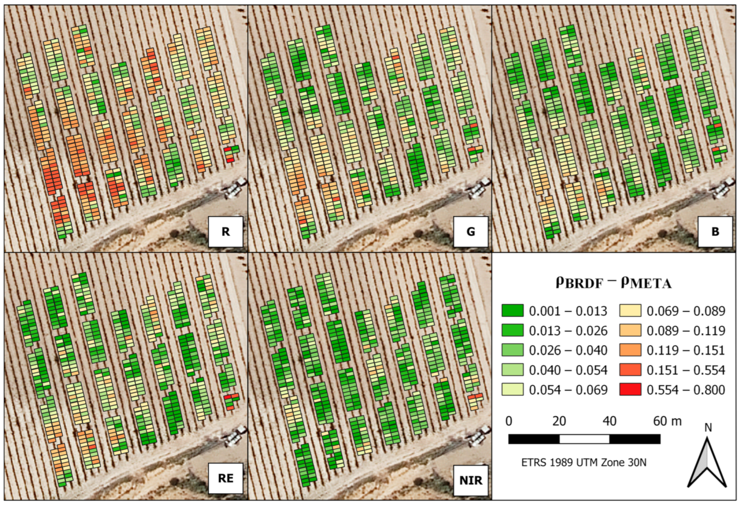
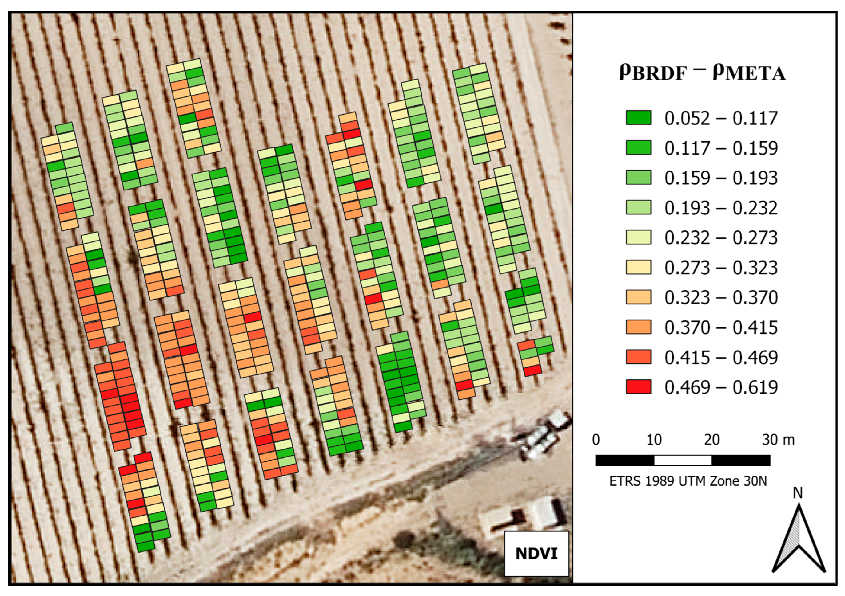
Spatial Analysis of the Differences

The distribution of the differences between the reflectances derived from the commercial software AgiSoft Metashape (ρMETA) and from the proposed methodology (ρBRDF) are represented in Figure 12. The colours signify the value of these differences. The red band shows the largest difference between methodologies among all bands, while considerable differences can be found in the green, blue, and red edge bands as well. The NIR band is the least affected by the proposed methodology.

As expected, the reflectance differences between the two methods used, especially for the red band, have a clear effect on the values calculated for NDVI, as can be seen in Figure 13.

4. Discussion

The increase in spatial resolution in remote sensing imagery, particularly in the case of UAV data, can lead to higher variance in observed reflectance values. This is attributed to the BRDF effect, which becomes more pronounced due to the greater variability in sun-surface-view geometry at higher spatial resolutions [8], specifically, this involves being able to see soil, sunlit, and shaded canopy elements individually. One of the contributing factors to this inconsistency is because the UAV views at a wider range of observation angles compared to the satellite. The orientation and angle of the leaves can significantly affect the reflectance values observed from different viewing angles and the sun’s position, leading to increased variability in the imagery. In addition, topographic effects have also been identified as a potential source of inconsistency in M_BRDF models. The topography of the study area can lead to variations in reflectance values based on the slope, aspect, and shadowing effects caused by the landscape and plant morphology.

The proposed methodological workflow provides a set of images with reflectances per band, according to the sensor manufacturer’s criteria, but taking into account hotspots, areas affected by shadows and BRDF effects. Furthermore, after the non-parametric ANOVA analysis, we can state that the reflectance products obtained using our M_BRDF correction model show statistically significant differences compared to common approaches. In this case, the reflectance values were provided by AgiSoft Metashape software. The Kruskal–Wallis H-test shows significant differences between the two methods across each spectral band (Table 6), as also observed in the Bonferroni post hoc analysis (Table A2, Appendix A). These differences can also be clearly seen in the box plot in Figure 10.

In addition, a detailed analysis of the magnitude of the differences between the reflectance data for the spectral bands considered in both methods shows that although the differences in the NIR band are not as large as those in the others, there are high value differences in the R band in particular, but there are also significant differences in the B, G and RE bands (Table 7). Given that the average difference in NDVI between the two methods is around 0.3, and that 75% of the data reach values up to 0.38 (Table 7), we can state that the NDVI is greatly affected by the M_BRDF correction when we compare both methodologies, since it is the R band, together with the NIR band, that is used to calculate this spectral index.

The proposed methodology involves the exclusive selection of the plant reflectance, with the removal of shadows and soil. As a result, the proposed methodology demonstrates superior homogeneity and more consistent values compared to Metashape for use in plant-only analysis. Metashape’s results include values that even hover around 0.2, which do not align with a healthy crop, as indicated in this study. The histogram shown in Figure 7 indicates that the NDVI values obtained from the reflectance data provided by Metashape tend to be homogeneous compared to those obtained using the M_BRDF correction model. This is due to the Metashape workflow, especially in orthomosaic acquisition, which uses colour normalization algorithms that incorporate geometry, altering the final reflectance values per band. On the other hand, it has to be taken into account that our methodology includes complex, high-level corrections that obtain reflectance values in a wider range, as can be clearly observed when comparing the histograms of reflectance values per band between the two methodologies (Figure 6a vs. Figure 6b). It is clear, therefore, that the proposed methodology, including the M_BRDF correction model, provides more consistent values temporally, and therefore, values for the NDVI that are more in line with our object of interest, the plant.

Finally, it is worth noting that there is an increase in the disparity of reflectance between both methodologies in the western area of the crop. The affected vines in this area are situated in a small valley (Figure 14), where terrain roughness and the presence of surrounding shadows significantly contribute to the enhancement of the BRDF effect, which, in turn, results in a noticeable influence on the recorded reflectance. The intrinsic relationship between topography and BRDF has been previously documented in the literature [42,43,44,45,46,47]. In this context, the western slope stands as an illustrative case of how the interaction between terrain morphology and environmental conditions can modulate the behaviour of the BRDF and, consequently, the reflectance in the study area. These findings underscore the importance of considering terrain roughness and topography when analysing and modelling BRDF behaviour in applications related to UAV-based remote sensing.

5. Conclusions

The need for quantitative, lightweight remote sensing applications using UAVs has been growing in environmental measurement and monitoring applications. In this study, a comprehensive processing workflow was developed for radiometric imaging that utilizes the MicaSense multispectral sensor onboard a UAV. The goal was to accurately and quantitatively assess agricultural fields, making the approach suitable for a wide range of agricultural monitoring applications, including crop health assessment, nutrient management, irrigation scheduling, and pest/disease detection.

Our results affirm the need to consider BRDF effects in understanding and mitigating brightness variations in UAV images caused by illumination and sensor geometries. Indeed, the fine-spatial scale characteristic of UAV imagery exacerbates the BRDF effect, necessitating its consideration in image processing and analysis. Past research has proposed the use of the Walthall BRDF model to address solar-viewing geometry variation. However, in more complex environments, such as those with varying topography and plant leaf angles, additional factors should be taken into account to accurately resolve solar-surface-viewing geometry variation [8].

UAV-captured high-precision information helps agronomists evaluate the response of the plant (only the plant) to different factors. It is known that the spectral response in the plant is dependent on the pigments that the plant contains. These pigments are also affected by the biotic and abiotic factors that affect the plants in their environment. Thus, evaluating vegetation indices at the leaf level represents a total improvement in the evaluation of plant status that can only be achieved with high-precision geomatic products such as those obtained with the use of drones. However, the response at leaf level to stress caused by biotic and abiotic factors is not too high, and any error in the measurement should be avoided. With the proposed methodology, we contribute to the decrease in error in the retrieval of plant-based indices.

The proposed methodology provides a better estimation of plant-only reflectances, translating into the consequent improvement in derived indices such as NDVI. This results in more accurate analysis-ready data for mapping and monitoring environmental changes in agronomical contexts. It does not produce an increase in field work. Current computer technology facilitates the application of the methodology in a very simple way and with reasonable processing times, using a computer program developed with open-source tools.

References

1. Jędrejek, A.; Pudełko, R. Exploring the Potential Use of Sentinel-1 and 2 Satellite Imagery for Monitoring Winter Wheat Growth under Agricultural Drought Conditions in North-Western Poland. Agriculture 2023, 13, 1798. [Google Scholar] [CrossRef]
2. Radočaj, D.; Šiljeg, A.; Marinović, R.; Jurišić, M. State of Major Vegetation Indices in Precision Agriculture Studies Indexed in Web of Science: A Review. Agriculture 2023, 13, 707. [Google Scholar] [CrossRef]
3. Xiong, Y.; Zhang, Z.; Fu, M.; Wang, L.; Li, S.; Wei, C.; Wang, L. Analysis of Vegetation Cover Change in the Geomorphic Zoning of the Han River Basin Based on Sustainable Development. Remote Sens. 2023, 15, 4916. [Google Scholar] [CrossRef]
4. Chi, J.; Kim, J.-I.; Lee, S.; Jeong, Y.; Kim, H.-C.; Lee, J.; Chung, C. Geometric and Radiometric Quality Assessments of UAV-Borne Multi-Sensor Systems: Can UAVs Replace Terrestrial Surveys? Drones 2023, 7, 411. [Google Scholar] [CrossRef]
5. Stow, D.; Nichol, C.J.; Wade, T.; Assmann, J.J.; Simpson, G.; Helfter, C. Illumination Geometry and Flying Height Influence Surface Reflectance and NDVI Derived from Multispectral UAS Imagery. Drones 2019, 3, 55. [Google Scholar] [CrossRef]
6. Osco, L.P.; Junior, J.M.; Ramos, A.P.M.; Jorge, L.A.d.C.; Fatholahi, S.N.; Silva, J.d.A.; Matsubara, E.T.; Pistori, H.; Gonçalves, W.N.; Li, J. A Review on Deep Learning in UAV Remote Sensing. Int. J. Appl. Earth Obs. Geoinf. 2021, 102, 102456. [Google Scholar] [CrossRef]
7. Miyoshi, G.T.; Arruda, M.d.S.; Osco, L.P.; Marcato Junior, J.; Gonçalves, D.N.; Imai, N.N.; Tommaselli, A.M.G.; Honkavaara, E.; Gonçalves, W.N. A Novel Deep Learning Method to Identify Single Tree Species in UAV-Based Hyperspectral Images. Remote Sens. 2020, 12, 1294. [Google Scholar] [CrossRef]
8. Bithas, P.S.; Michailidis, E.T.; Nomikos, N.; Vouyioukas, D.; Kanatas, A.G. A Survey on Machine-Learning Techniques for UAV-Based Communications. Sensors 2019, 19, 5170. [Google Scholar] [CrossRef]
9. Bouguettaya, A.; Zarzour, H.; Kechida, A.; Taberkit, A.M. Deep Learning Techniques to Classify Agricultural Crops through UAV Imagery: A Review. Neural Comput. Appl. 2022, 34, 9511–9536. [Google Scholar] [CrossRef]
10. López-García, P.; Intrigliolo, D.; Moreno, M.A.; Martínez-Moreno, A.; Ortega, J.F.; Pérez-Álvarez, E.P.; Ballesteros, R. Machine Learning-Based Processing of Multispectral and RGB UAV Imagery for the Multitemporal Monitoring of Vineyard Water Status. Agronomy 2022, 12, 2122. [Google Scholar] [CrossRef]
11. Agisoft Metashape: Agisoft Metashape. Available online: https://www.agisoft.com/ (accessed on 18 October 2023).
12. Herrero-Huerta, M.; Felipe-García, B.; Belmar-Lizarán, S.; Hernández-López, D.; Rodríguez-Gonzálvez, P.; González-Aguilera, D. Dense Canopy Height Model from a Low-Cost Photogrammetric Platform and LiDAR Data. Trees 2016, 30, 1287–1301. [Google Scholar] [CrossRef]
13. Tucker, C.J. Spectral estimation of grass canopy variables. Remote Sens. Environ. 1977, 6, 11–26. [Google Scholar] [CrossRef]
14. Ortega-Terol, D.; Hernandez-Lopez, D.; Ballesteros, R.; Gonzalez-Aguilera, D. Automatic Hotspot and Sun Glint Detection in UAV Multispectral Images. Sensors 2017, 17, 2352. [Google Scholar] [CrossRef]
15. Tu, Y.-H.; Phinn, S.; Johansen, K.; Robson, A. Assessing Radiometric Correction Approaches for Multi-Spectral UAS Imagery for Horticultural Applications. Remote Sens. 2018, 10, 1684. [Google Scholar] [CrossRef]
16. Verger i Ten, A.; Camacho-de Coca, F.; Melía, J. Revisión de los modelos paramétricos de BRDF. Rev. Teledetec. Rev. Asoc. Esp. Teledetec. 2005, 23, 65–80. [Google Scholar]
17. Kim, M.; Jin, C.; Lee, S.; Kim, K.-M.; Lim, J.; Choi, C. Calibration of BRDF Based on the Field Goniometer System Using a UAV Multispectral Camera. Sensors 2022, 22, 7476. [Google Scholar] [CrossRef]
18. Pan, Z.; Zhang, H.; Min, X.; Xu, Z. Vicarious Calibration Correction of Large FOV Sensor Using BRDF Model Based on UAV Angular Spectrum Measurements. J. Appl. Remote Sens. 2020, 14, 027501. [Google Scholar] [CrossRef]
19. St»hle, L.; Wold, S. Analysis of Variance (ANOVA). Chemom. Intell. Lab. Syst. 1989, 6, 259–272. [Google Scholar] [CrossRef]
20. Pour-Aboughadareh, A.; Mohammadi, R.; Etminan, A.; Shooshtari, L.; Maleki-Tabrizi, N.; Poczai, P. Effects of Drought Stress on Some Agronomic and Morpho-Physiological Traits in Durum Wheat Genotypes. Sustainability 2020, 12, 5610. [Google Scholar] [CrossRef]
21. Calamai, A.; Masoni, A.; Marini, L.; Dell’acqua, M.; Ganugi, P.; Boukail, S.; Benedettelli, S.; Palchetti, E. Evaluation of the Agronomic Traits of 80 Accessions of Proso Millet (Panicum miliaceum L.) under Mediterranean Pedoclimatic Conditions. Agriculture 2020, 10, 578. [Google Scholar] [CrossRef]
22. Azad, A.K.; Sarker, U.; Ercisli, S.; Assouguem, A.; Ullah, R.; Almeer, R.; Sayed, A.A.; Peluso, I. Evaluation of Combining Ability and Heterosis of Popular Restorer and Male Sterile Lines for the Development of Superior Rice Hybrids. Agronomy 2022, 12, 965. [Google Scholar] [CrossRef]
23. Serrano, A.S.; Martínez-Gascueña, J.; Alonso, G.L.; Cebrián-Tarancón, C.; Carmona, M.D.; Mena, A.; Chacón-Vozmediano, J.L. Agronomic Response of 13 Spanish Red Grapevine (Vitis vinifera L.) Cultivars under Drought Conditions in a Semi-Arid Mediterranean Climate. Agronomy 2022, 12, 2399. [Google Scholar] [CrossRef]
24. IGN. Atlas Nacional de España. Clima. Available online: http://atlasnacional.ign.es/wane/Clima (accessed on 18 October 2023).
25. MicaSense Knowledge Base. Available online: https://support.micasense.com/hc/en-us (accessed on 18 October 2023).
26. Taddia, Y.; Russo, P.; Lovo, S.; Pellegrinelli, A. Multispectral UAV Monitoring of Submerged Seaweed in Shallow Water. Appl. Geomat. 2020, 12, 19–34. [Google Scholar] [CrossRef]
27. Hernandez-Lopez, D.; Felipe-Garcia, B.; Gonzalez-Aguilera, D.; Arias-Perez, B. An Automatic Approach to UAV Flight Planning and Control for Photogrammetric Applications. Photogramm. Eng. Remote Sens. 2013, 79, 87–98. [Google Scholar] [CrossRef]
28. MicaSense RedEdge MX Processing Workflow (Including Reflectance Calibration) in Agisoft Metashape Professional. Available online: https://agisoft.freshdesk.com/support/solutions/articles/31000148780-micasense-rededge-mx-processing-workflow-including-reflectance-calibration-in-agisoft-metashape-pro (accessed on 18 October 2023).
29. Walthall, C.L.; Norman, J.M.; Welles, J.M.; Campbell, G.; Blad, B.L. Simple Equation to Approximate the Bidirectional Reflectance from Vegetative Canopies and Bare Soil Surfaces. Appl. Opt. 1985, 24, 383–387. [Google Scholar] [CrossRef] [PubMed]
30. Strahler, A.; Lucht, W.; Schaaf, C.; Tsang, T.; Gao, F.; Muller, J. MODIS BRDF/Albedo Product: Algorithm Theoretical Basis Document Version 5.0. MODIS Doc. 1999, 23, 42–47. [Google Scholar]
31. MicaSense GitHub. Available online: https://micasense.github.io/imageprocessing/index.html (accessed on 18 October 2023).
32. Cardinal, R.N.; Aitken, M.R.F. ANOVA for the Behavioral Sciences Researcher; Psychology Press: London, UK, 2013; ISBN 978-1-134-81410-7. [Google Scholar]
33. Strunk, K.K.; Mwavita, M. Design and Analysis in Educational Research: ANOVA Designs in SPSS®; Routledge: London, UK, 2020; ISBN 978-0-429-78006-6. [Google Scholar]
34. Rosner, B.; Grove, D. Use of the Mann–Whitney U-Test for Clustered Data. Stat. Med. 1999, 18, 1387–1400. [Google Scholar] [CrossRef]
35. McKnight, P.E.; Najab, J. Mann-Whitney U Test. In The Corsini Encyclopedia of Psychology; John Wiley & Sons, Ltd.: Hoboken, NJ, USA, 2010; p. 1. ISBN 978-0-470-47921-6. [Google Scholar]
36. Vargha, A.; Delaney, H.D. The Kruskal-Wallis Test and Stochastic Homogeneity. J. Educ. Behav. Stat. 1998, 23, 170–192. [Google Scholar] [CrossRef]
37. Ostertagová, E.; Ostertag, O.; Kováč, J. Methodology and Application of the Kruskal-Wallis Test. Appl. Mech. Mater. 2014, 611, 115–120. [Google Scholar] [CrossRef]
38. Yuen, K.K. The Two-Sample Trimmed t for Unequal Population Variances. Biometrika 1974, 61, 165–170. [Google Scholar] [CrossRef]
39. Luh, W.-M.; Guo, J.-H. A Powerful Transformation Trimmed Mean Method for One-Way Fixed Effects ANOVA Model under Non-Normality and Inequality of Variances. Br. J. Math. Stat. Psychol. 1999, 52, 303–320. [Google Scholar] [CrossRef]
40. Cabin, R.J.; Mitchell, R.J. To Bonferroni or Not to Bonferroni: When and How Are the Questions. Bull. Ecol. Soc. Am. 2000, 81, 246–248. [Google Scholar]
41. TIDOP-USAL/ANOVA_BRDF: Non-Parametrical ANOVA Analysis for the BRDF. Available online: https://github.com/TIDOP-USAL/ANOVA_BRDF (accessed on 23 October 2023).
42. Wen, J.; Liu, Q.; Xiao, Q.; Liu, Q.; You, D.; Hao, D.; Wu, S.; Lin, X. Characterizing Land Surface Anisotropic Reflectance over Rugged Terrain: A Review of Concepts and Recent Developments. Remote Sens. 2018, 10, 370. [Google Scholar] [CrossRef]
43. Guo, Y.; Jia, X.; Paull, D. Superpixel-Based Adaptive Kernel Selection for Angular Effect Normalization of Remote Sensing Images With Kernel Learning. IEEE Trans. Geosci. Remote Sens. 2017, 55, 4262–4271. [Google Scholar] [CrossRef]
44. Schaaf, C.B.; Li, X.; Strahler, A.H. Topographic Effects on Bidirectional and Hemispherical Reflectances Calculated with a Geometric-Optical Canopy Model. IEEE Trans. Geosci. Remote Sens. 1994, 32, 1186–1193. [Google Scholar] [CrossRef]
45. Petach, A.R.; Toomey, M.; Aubrecht, D.M.; Richardson, A.D. Monitoring vegetation phenology using an infrared-enabled security camera. Agric. For. Meteorol. 2014, 195, 143–151. [Google Scholar] [CrossRef]
46. Filippa, G.; Cremonese, E.; Migliavacca, M.; Galvagno, M.; Sonnentag, O.; Humphreys, E.; Hufkens, K.; Ryu, Y.; Verfaillie, J.; di Cella, U.M.; et al. NDVI derived from near-infrared-enabled digital cameras: Applicability across different plant functional types. Agric. For. Meteorol. 2018, 249, 275–285. [Google Scholar] [CrossRef]
47. Honkavaara, E.; Saari, H.; Kaivosoja, J.; Pölönen, I.; Hakala, T.; Litkey, P.; Mäkynen, J.; Pesonen, L. Processing and Assessment of Spectrometric, Stereoscopic Imagery Collected Using a Lightweight UAV Spectral Camera for Precision Agriculture. Remote Sens. 2013, 5, 5006–5039. [Google Scholar] [CrossRef]
Figure 1. Study area: vineyard located in Fuente Alamo (Albacete, Spain).
Drones 08 00036 g001
Figure 2. UAV used in this study (Carabo S3).
Drones 08 00036 g002
Figure 3. Ground control points (GCPs) located in the case study.
Drones 08 00036 g003
Figure 4. Proposed methodology, which includes BRDF correction.
Drones 08 00036 g004
Figure 5. Statistical analysis workflow.
Drones 08 00036 g005
Figure 6. Histogram of the reflectance values, including the theoretical normal distribution for each spectral band. (a) M_BRDF methodology; (b) data provided by Metashape.
Drones 08 00036 g006
Figure 7. Histogram of the NDVI values, including the theoretical normal distribution, considering the mean and std for each method.
Drones 08 00036 g007
Figure 8. QQ Plots: (a) M_BRDF reflectances; (b) M_BRDF NDVI; (c) Metashape reflectances; (d) Metashape NDVI.
Drones 08 00036 g008
Figure 9. Box plot graph comparing methodologies: (a) reflectance data; (b) NDVI data.
Drones 08 00036 g009
Figure 10. Box plot graph comparing the reflectance data per band for each method.
Drones 08 00036 g010
Figure 11. Histogram of difference between Metashape and M_BRDF data: (a) reflectance band data; (b) NDVI data.
Drones 08 00036 g011
Figure 12. Spatial distribution of the absolute value of the differences between reflectances derived from the proposed methodology (ρBRDF) and from the commercial software AgiSoft Metashape (ρMETA) per band (R = red, G = green, B = blue, RE = red edge and NIR = near infrared).
Drones 08 00036 g012
Figure 13. Spatial distribution of the absolute differences in NDVI values, obtained from the reflectances derived from the proposed methodology (ρBRDF) and the commercial software AgiSoft Metashape (ρMETA).
Drones 08 00036 g013
Figure 14. Spatial distribution of the absolute values of the NDVI differences between both methods, integrating the topography through the DTM.
Drones 08 00036 g014