1. Introduction
The prevailing research in the field of Unmanned Combat Aerial Vehicles (UCAVs) is centered on enhancing autonomy, which necessitates advanced intelligent decision-making capabilities. To effectively navigate dynamic air combat game environments, a UCAV must execute swift and informed decisions. Traditional methods like the differential game method [
1,
2], influence diagram method [
3,
4], model predictive control [
5], genetic algorithms [
6], and Bayesian inference [
7] have been deployed to tackle tactical decision-making challenges. These approaches analyze relationships in air combat games to derive optimal solutions but often falter in complex environments that require real-time calculations.
With the increasing complexity of air combat game scenarios, decision-making strategies must evolve. Recently, artificial intelligence (AI) has shown promise in addressing these challenges, particularly through its capability for real-time performance. Traditional AI methods include expert systems, which utilize comprehensive rule bases to generate empirical policies [
8,
9,
10,
11], and supervised learning, which employs neural networks to translate sensor data into tactical decisions based on expert demonstrations [
12,
13,
14]. However, these methods are limited by their reliance on hard-to-obtain expert data, which may not adequately represent the complexities of real-world air combat games.
Reinforcement Learning (RL) addresses these limitations by enabling autonomous learning through environmental interactions, thus maximizing returns without prior expertise [
15]. This approach has gained traction in autonomous air combat game applications, where UCAVs operate as agents [
16,
17,
18,
19,
20]. Pioneers like McGrew [
21] and Crumpacker [
22] have applied approximate dynamic programming to develop maneuver decision models for 1 vs. 1 air combat game scenarios, with McGrew even testing these on micro-UCAVs. Their work underscores the viability of RL in autonomous tactical decision-making. Additional advancements include efforts by Xiaoteng Ma [
23], who integrated speed control into the action space using Deep Q-Learning, and Zhuang Wang [
24], who introduced a freeze game framework to mitigate nonstationarity in RL through a league system that adapts to varying opponent strategies. Furthermore, Qiming Yang [
25] developed a motion model for a second-order UCAV and a close-range air combat game model in 3D, employing DQN and basic confrontation training techniques. Notably, Adrian’s use of Hierarchical RL [
26] secured a second-place finish in DARPA’s AlphaDogfight Trials, showcasing the effectiveness of artificially aided rewards in challenging air combat game scenarios.
Despite these advancements, the sparse reward challenge in RL persists, especially in high-dimensional settings like air combat games, where agents must identify a sequence of correct actions to attain the sparse reward. Traditional random exploration often proves inadequate, which provides minimal feedback on action quality. In response, scholars have explored various strategies, including reward shaping [
27,
28,
29], curriculum learning [
30,
31,
32], learning from demonstrations [
33,
34,
35], model-guided learning [
36], and inverse RL [
37]. However, these methods typically rely on artificial prior knowledge, potentially biasing policies toward suboptimal outcomes.
Furthermore, previous studies often oversimplify air combat game scenarios, assuming 2D movement or discretized basic flight maneuvers (BFM), thus hampering the realism and efficacy of learned policies. In contrast, this paper advances the following contributions:
- (1)
We introduce the homotopy-based soft actor–critic (HSAC) algorithm to address the sparse reward problem in air combat games. We theoretically validate the feasibility and consistent convergence of this approach, offering a new perspective for RL-based methods.
- (2)
We develop a more realistic air combat game environment, utilizing a refined 3D flight dynamics model and expanding the agent’s action space from discrete to continuous.
- (3)
We implement the HSAC algorithm in this enhanced environment, leveraging self-play. Simulations demonstrate that HSAC significantly outperforms models trained with either sparse or artificially aided rewards.
The paper is structured as follows:
Section 2 reviews existing RL-based methods and introduces the air combat game problem.
Section 3 details our air combat game environment setup, incorporating a refined 3D flight dynamics model and a continuous action space. In
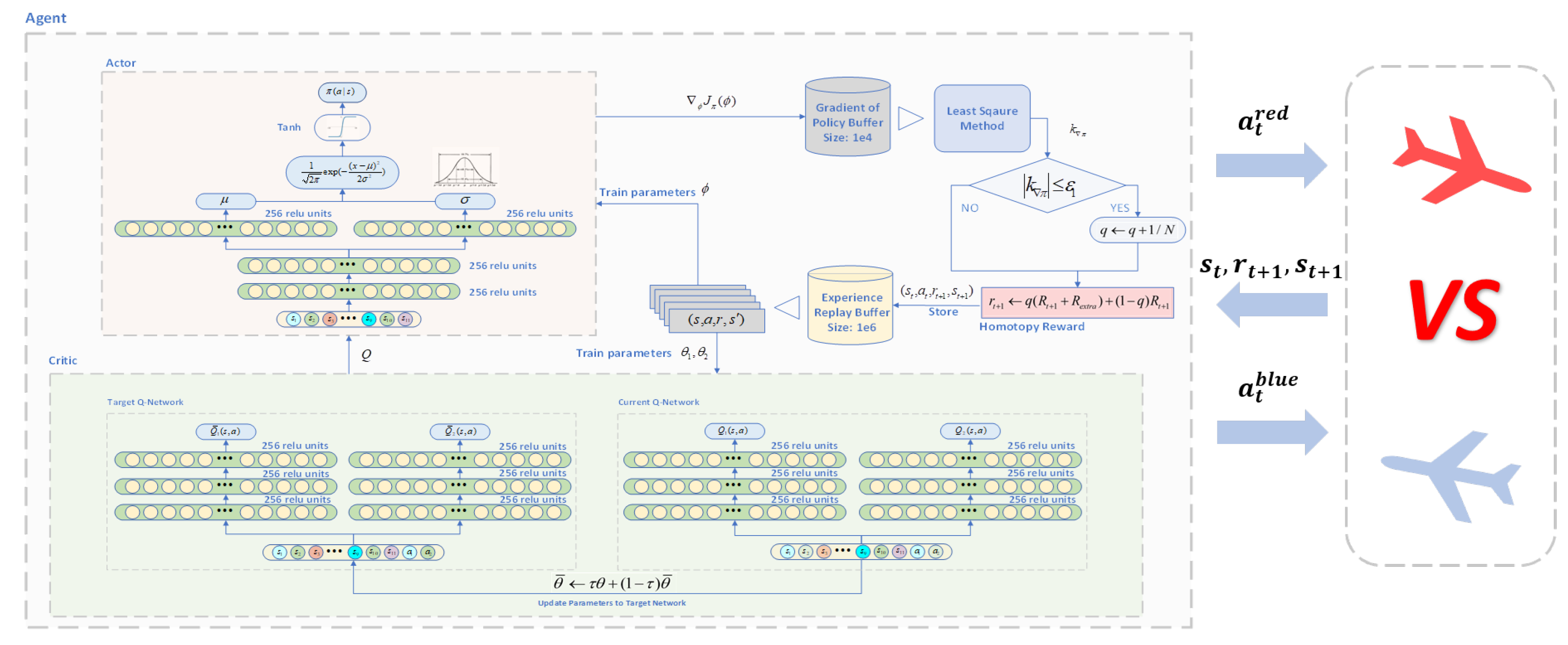
Section 4, we describe the homotopy-based soft actor–critic algorithm and provide theoretical evidence of its convergence and effectiveness. An overview diagram of the HSAC algorithm is shown in
Figure 1.
Section 5 showcases the performance of the HSAC algorithm in various training and experimental setups. Links to video footage of the training process are available online (
Supplementary Materials). Finally,
Section 6 summarizes our contributions and discusses future research directions.
2. Preliminaries
In this section, we provide an overview of the dynamics model of a UCAV during short-range air combat game scenarios and introduce the soft actor–critic (SAC) method, a widely recognized reinforcement learning (RL) algorithm for training autonomous agents.
2.1. One-to-One Short-Range Air Combat Game Problem
Short-range air combat games, also known as dogfights, entail the objective of shooting down an enemy UCAV while avoiding return fire. To distinguish between the UCAVs of opposing sides, we use superscript b for blue-side UCAVs and superscript r for red-side UCAVs. The interaction between and is inherently adversarial. For simplicity, our focus will primarily be on the learning problem of .
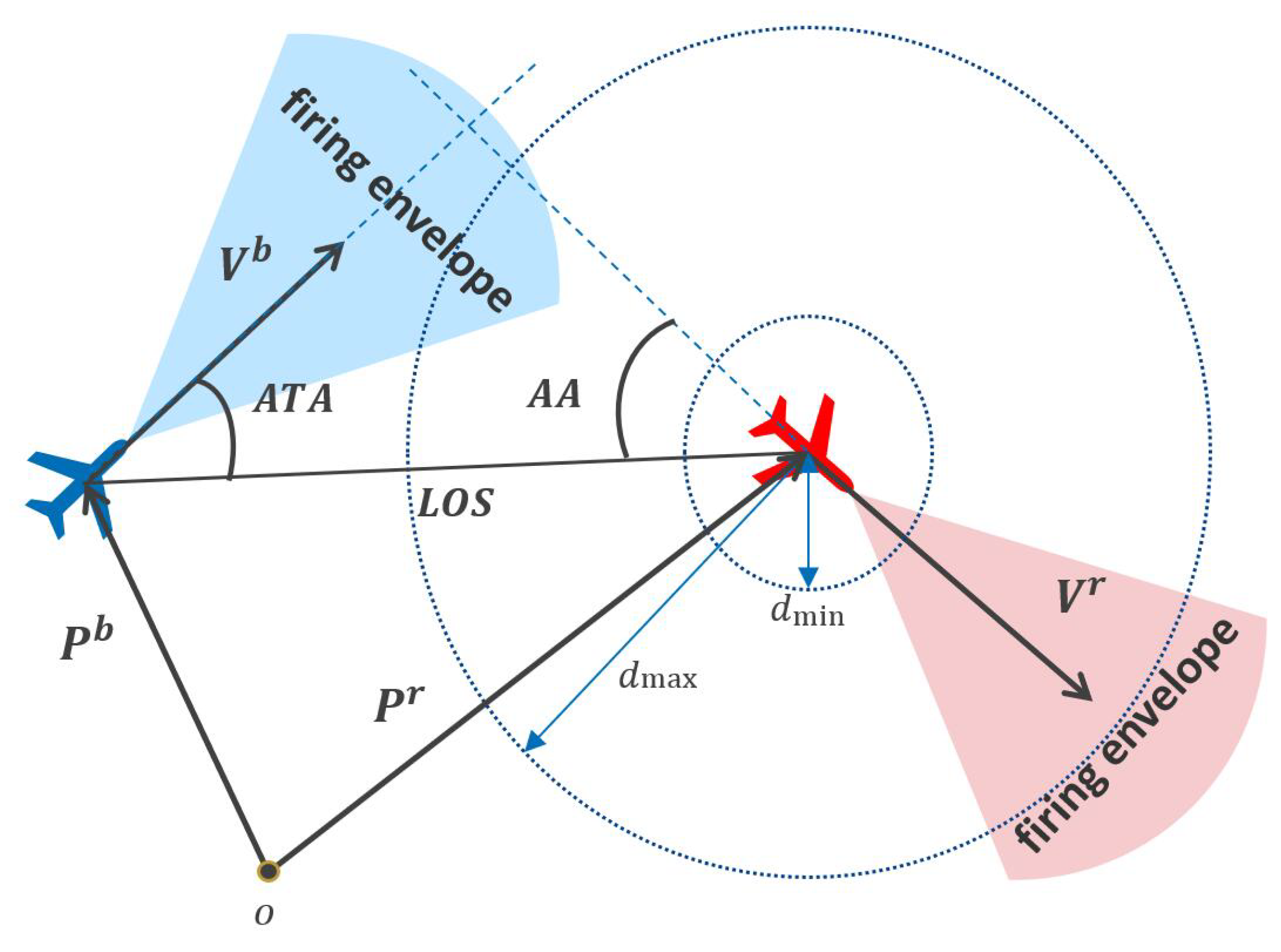
Figure 2 illustrates a typical one-to-one short-range air combat game scenario. In this model, four variables are crucial for defining the advantageous position of
: Aspect Angle (AA), Antenna Train Angle (ATA), Line of Sight (LOS), and Relative Distance. These metrics allow
to determine the position
and velocity
of the opposing
.
For to successfully engage , it must fulfill the following criteria:
- (1)
The relative distance between the UCAVs must be within the maximum attack range and above the minimum collision range.
- (2)
must maintain an advantageous position, enabling the pursuit of while evading potential counterattacks.
These requirements are governed by the following constraints [
21]:
If all constraints in Equation (1) are satisfied,
can engage
within its firing envelope [
38]. The same operational constraints apply to
.
A two-target differential game model [
39,
40] aptly describes this air combat game scenario:
Here,
and
denote the control policies of each UCAV, whereas
and
represent their respective state vectors, as defined in Equation (3). In Equation (2),
and
are the loss functions for
and
, respectively, with
representing the terminal punishment function:
Here,
v,
,
represents the velocity, the flight path angle, and the heading angle of UCAV.
The primary aim of this research is to enable
to rapidly attain an advantageous position. In reinforcement learning, the concept of self-play is often utilized to simplify the adversarial game, a strategy that has been successfully implemented in AlphaZero [
41]. Consequently, we have simplified the two-target differential game into an optimization problem that satisfies the UCAV dynamics constraints. More details are provided in
Section 4.4.
2.2. UCAV’s Dynamics Model
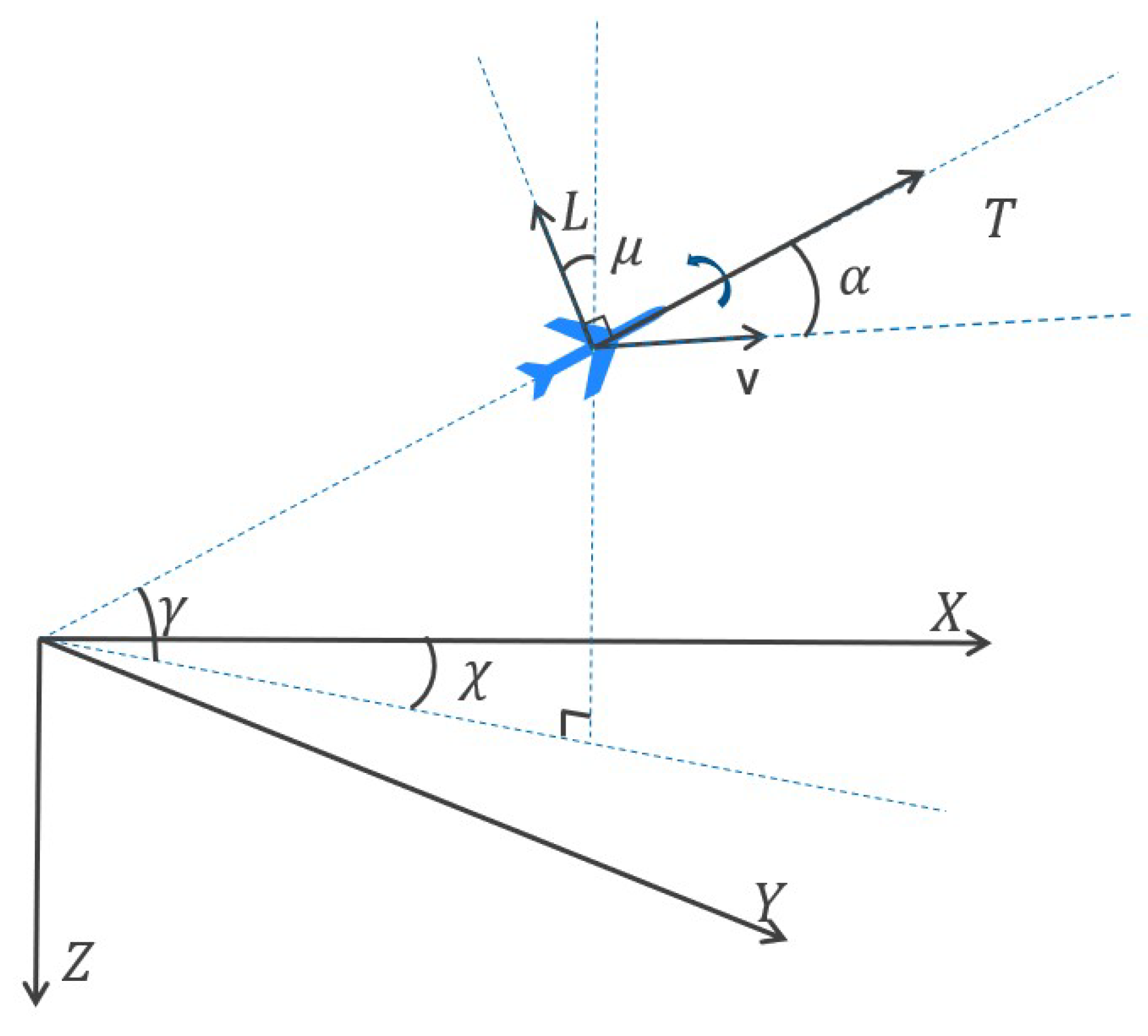
The dynamics model of the UCAV is crucial for accurately simulating air combat game scenarios and is constructed using the ground coordinate system. This model is described by a three-degree-of-freedom (3-DoF) particle motion model [
3]:
In Equation (4),
,
, and
denote the UCAV’s rates of change in position along the
X,
Y, and
Z axes, respectively. The variables
,
, and
v represent the flight path angle, heading angle, and velocity, respectively.
Figure 3 illustrates the associated flight dynamics.
Control variables for the UCAV, including the attack angle
, throttle setting
, and bank angle
, interplay intricately via:
Here,
g,
m, and
represent the acceleration due to gravity, the mass of the UCAV, and the maximum thrust force of the engine, respectively. Lift and drag forces are given as follows:
Here, the reference wing area is denoted by
. The air density
is assumed to be a constant in this study.
and
denote lift and drag coefficients, respectively, related through the attack angle
:
Variables
,
,
, and
in Equation (7) signify the zero-lift coefficient, the derivative of the lift coefficient with respect to attack angle, zero-drag coefficient, and the drag–lift coefficient, respectively.
Constraints on both the control variables and their rate of change are defined to ensure performance and maintain UCAV inertia within operational limits:
The throttle setting
is assumed constant at 1 to maximize pursuit capabilities.
The load factor
and dynamic pressure
are defined as follows:
Constraints on these parameters prevent overloading of the UCAV:
where
,
, and
denote the minimum altitude, maximum load factor, and maximum dynamic pressure, respectively. Additionally, it is important to note that the relationship between altitude
h and the functions
and
is not considered here, as the air density
is assumed constant.
2.3. Soft Actor–Critic Method
The Markov Decision Process (MDP) is fundamental to RL-based methods, facilitating the modeling of sequential decision-making problems using mathematical formalism. An MDP consists of a state space S, an action space A, a transition function T, and a reward function R, forming a tuple . RL-based methods aim to optimize the agent’s policy through interaction with the environment. At each time step t, the agent in state chooses an action , and the environment provides feedback on the next state based on the transition probability , along with a reward to evaluate the quality of the action. The policy directs the agent’s action selection in each state, with the probability of each action given by . The ultimate objective is to discover an optimal policy that maximizes the expected cumulative reward.
Finding the optimal policy
can be challenging, especially if the agent has not extensively explored the state space. This challenge is addressed by employing maximum entropy reinforcement learning techniques, such as the soft actor–critic (SAC) algorithm [
42]. SAC is a model-free, off-policy RL algorithm that integrates policy entropy into the objective function to encourage exploration across various states [
43]. Recognized for its effectiveness, SAC has become a benchmark algorithm in RL implementations, outperforming other advanced methods like SQL [
44] and TD3 [
45] across multiple environments [
42,
46].
The optimal policy
is described as follows:
Here,
denotes the entropy of the action distribution at state
, and
is the distribution of the agent’s initial state. The discount factor
balances the importance of immediate versus future rewards, and
is the temperature parameter that influences the algorithm’s convergence.
Following the Bellman Equation [
15], the soft Q-function is expressed as follows:
The soft value function is derived from the soft Q-function:
The parameters of the soft Q-function are trained to minimize the temporal difference (TD) error, whereas the policy parameters minimize the Kullback-Leibler divergence between the normalized soft Q-function and the policy distribution.
The critic network’s loss function is defined as follows:
The actor network’s loss function, simplifying the actor’s learning objective, is given in Equation (15):
To manage the sensitivity of the hyperparameter
, an automatic adjustment technique is proposed, framing the problem within a maximum entropy RL paradigm with a minimum entropy constraint. This approach, outlined in Equation (16), employs a neural network to approximate
, targeting a desired minimum expected entropy
:
3. Configuration of One-to-One Air Combat Game in RL
This section outlines the environment setup required for applying RL-based methods to the air combat game optimization problem specified in Equation (2). The environment encapsulates the state space, action space, transition function, and reward function. We also discuss the transformation of the global state space into a relative state space, which simplifies the representation of state information for UCAVs significantly.
3.1. Action Space
The control laws for UCAVs, denoted as
and
, are represented by the vector format in Equation (17):
Constraints on these control variables are defined in Equation (8). The action vectors, which influence the control variables, are designed as shown in Equation (18):
These action vectors modify the control laws at each timestep as outlined in Equation (19), where constraints ensure the actions remain within feasible limits:
and
are the initial attack angle and initial bank angle of the UCAV, respectively.
3.2. State Space
A well-designed state space can facilitate faster convergence of learning algorithms. Referring to [
47], the state space for each UCAV can initially be represented as follows:
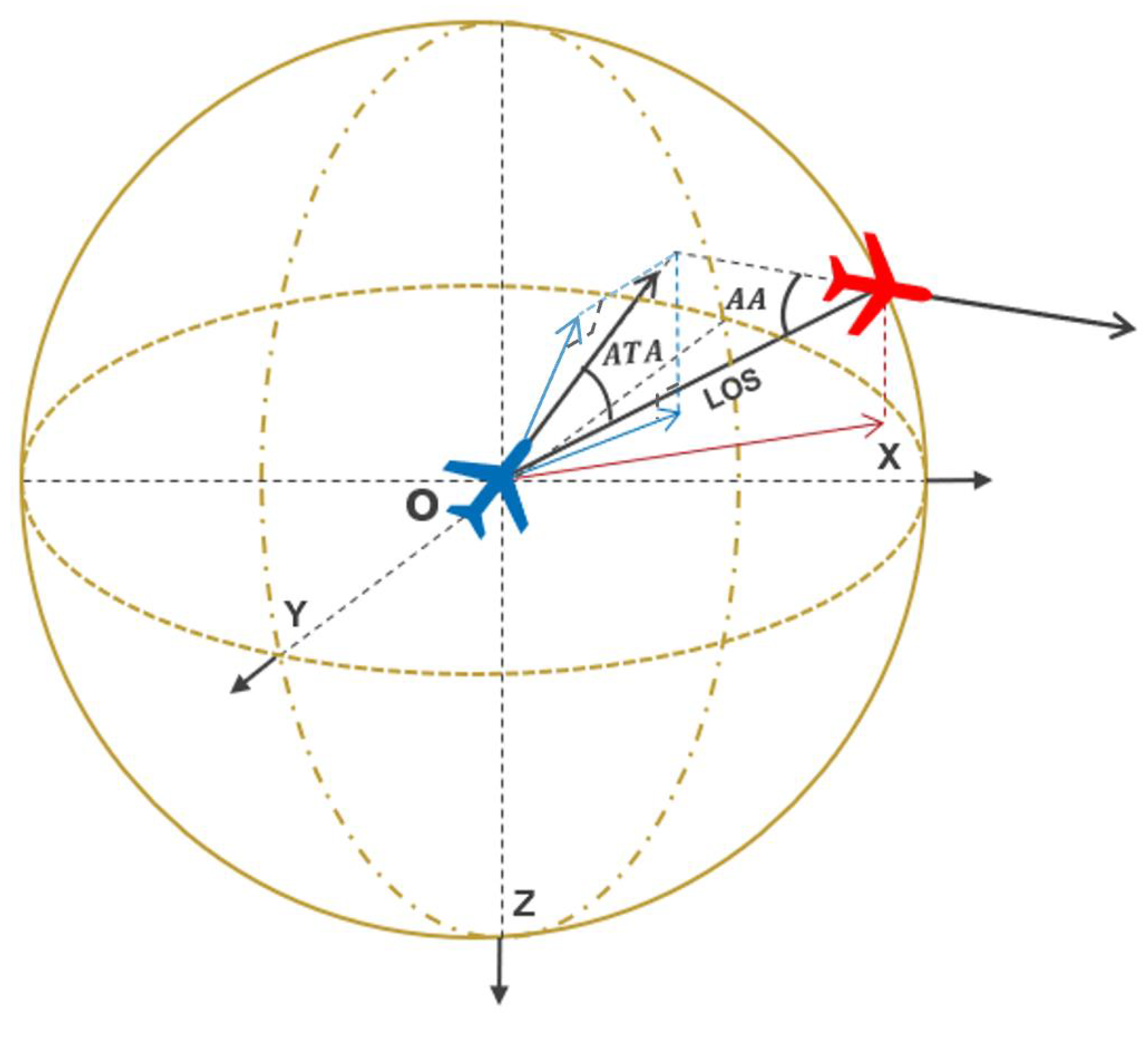
To reduce the dimensionality and simplify this state information, we transform the global state into a relative state for each UCAV as follows:
The angle projection onto the
and
planes, as illustrated in
Figure 4, are denoted by the subscripts
and
, respectively.
represents the line of sight distance between the UCAVs. Additionally, we normalize the state variables to facilitate neural network processing, ensuring learning efficiency:
3.3. Transition Function
To improve the accuracy of our simulation results, we employ the fourth-order Runge-Kutta method [
48] for solving the differential equation described in
Section 2.2. The specifics of this method are presented in Equation (25), ensuring precise integration of the UCAV dynamics:
where we consider the system of equations
, with initial condition
. In this context, the function
denotes the rate of change of
when the agent chooses the action
a at the time step
t.
This method accounts for the nonlinear dynamics of the UCAVs, providing a robust framework for accurate state predictions over the simulation timeframe.
3.4. Reward
In this study, we categorize scenarios involving UCAVs based on Algorithm 1. This classification serves as the foundation for constructing the reward function for
, as detailed in Equation (26).
This reward structure incentivizes
to achieve a tactically advantageous position, granting a win reward of
. Should
become overloaded while
remains operational,
is deemed the winner and receives a reward of
. Conversely, if a UCAV is either killed or becomes overloaded, it incurs a penalty of
. Additionally, to encourage expeditious resolution of engagements, a time penalty of
is applied to each UCAV until the end of the game.
Figure 5 visually represents the logical framework of the environment.
| Algorithm 1 Air combat game criterion of |
Input: State:
Output: Situation of UCAV in air combat game:
- 1:
: Euclidean distance between UCAV - 2:
if then - 3:
- 4:
else if and and then - 5:
- 6:
else if and and then - 7:
- 8:
else - 9:
- 10:
end if
|
4. Homotopy-Based Soft Actor–Critic Method
Learning a policy for achieving an advantageous posture using only sparse rewards and random exploration is a formidable challenge for any agent. Alternatively, relying solely on artificial prior knowledge may prevent the discovery of the optimal policy. To navigate these challenges, we propose a novel homotopy-based soft actor–critic (HSAC) algorithm that leverages the benefits of both artificial prior knowledge and a sparse reward formulation. Initially, the algorithm employs artificial prior knowledge to establish a suboptimal policy. Subsequently, it follows a homotopic path in the solution space, guiding a sequence of suboptimal policies to converge toward the optimal policy. This method effectively balances exploration and exploitation, leading to a robust policy capable of securing an advantageous posture.
4.1. Homotopy-Based Reinforcement Learning
The challenge of reinforcement learning with sparse rewards, denoted as
R, is modeled as a nonlinear programming (NLP) problem, referred to as
NLP1, following the framework proposed by Bertsekas [
49].
Here,
, and
denotes the parameters of the actor network. The functions
and
correspond to the environment’s equality and inequality constraints, respectively.
To address the sparse reward challenge in reinforcement learning, researchers often introduce artificial priors that generate an additional reward signal,
, to aid agents in policy discovery [
23,
24,
25]. This enhancement improves the feedback on the agent’s actions at each step, facilitating learning. Thus, we define the total reward as the sum of
R and
, and formulate the enhanced reinforcement learning problem as
NLP2.
The feasible policy derived from
NLP2 is not the optimal solution to
NLP1 due to distortions caused by the artificial priors. To achieve convergence to the optimal solution of the original problem, we recommend a gradual transition using homotopy. We introduce a function operator
:
where
. This function operator facilitates the formulation of a homotopy NLP problem as depicted in
NLP3.
By adjusting q from 0 to 1, we can derive a continuous set of solutions transitioning from the solution to NLP2 to the solution to NLP1.
We propose a homotopic reward function,
, that integrates both sparse and extra rewards proportionally based on
q:
The equivalence of maximizing the expected accumulated homotopic reward
to solving the
NLP3 problem is demonstrated in Theorem 1, with proof provided in
Appendix A.
Theorem 1. equals to the expectation of accumulated homotopic reward as shown in Equation (30). 4.2. Homotopic Path Following with Predictor–Corrector Method
The solution to the auxiliary problem (NLP2) can be seamlessly transformed into the solution for the original problem (NLP1) using the function , as assured by Theorem 2.
Theorem 2. Under Assumption A1, a continuous homotopic path necessarily exists between the solutions to NLP2 and NLP1.
Here, a “path” denotes a piecewise differentiable curve within the solution space. The proof for the existence of this homotopic path is provided in
Appendix B.
This section utilizes a classical method known as the horizontal corrector and elevator predictor [
50] to navigate from a feasible solution toward the optimal solution for the original problem (
NLP1), tracing the homotopic path in the solution space.
Initially, we identify the auxiliary problem (NLP2) as and label the original problem (NLP1) as . The goal of is to determine the optimal policy , maximizing cumulative reward. Theoretically, by following a feasible homotopic path, we can transition to obtaining the optimal policy for the original task.
Additionally, we introduce a parameter N, representing the number of steps required for q to complete the transition from the auxiliary to the original solution. This sequence is defined by , where . This definition allows for a sequence of corresponding sub-tasks , where . The pair consisting of the parameter of the actor network and the value of q at step n is denoted as .
4.2.1. Predictor
If the optimal policy
has been determined for task
at step
n, we can predict the parameter
for the subsequent optimal policy
on the homotopic path using the elevator predictor approach [
50], as shown in Equation (31).
4.2.2. Corrector
After predicting for the new task , the predicted parameter tuple may not exactly align with the homotopic path. To re-align, the corrector step adjusts the predicted tuple back to the true solution tuple using a technique known as the horizontal corrector. During this correction, remains constant.
The solution’s accuracy is the sole focus during this process, as RL-based methods inherently manage correction through gradient descent. The convergence criteria are established by the transformation of the homotopy problem (
NLP3) into the condition
, with the precise conditions detailed in
Appendix B.
Here, denotes the convergence threshold for the criterion.
4.3. Algorithm
The convergence proof for the predictor–corrector path-following method is delineated in
Appendix B, and Theorem 3 posits the following principle:
Theorem 3. As the parameter transitions from 0 to 1 using the horizontal corrector and elevator predictor methods, the solution for task may converge to the optimal solution for task .
Inspired by this theorem, we have developed the homotopy-based soft actor–critic (HSAC) algorithm, which is encapsulated in Algorithm 2. This approach utilizes the variance trend of the parameter within the actor network of the SAC algorithm, denoted as , to assess policy convergence. The slope of the policy gradient’s changes is computed by fitting the policy gradient data to a first-order function using the least squares method, subsequently utilizing this slope to evaluate the quality of convergence within task .
Algorithm 2 includes a buffer, , to store the gradient of the policy for computing . M denotes the sample size for the least squares method, while N represents the total number of iterations required for the homotopy method.
During the horizontal corrector step, the policy parameter within is iteratively adjusted to approximate the optimal policy for task . If the slope meets the criterion , the corrector step is completed. Otherwise, the iteration of the policy parameter continues.
The elevator predictor step begins by clearing the policy gradient buffer to accommodate new data for the subsequent task . The parameter from the optimal policy of the preceding task is directly transferred to the policy for the new task .
This structured approach ensures rapid convergence to a feasible policy for the initial task
using the additional reward
at the training’s commencement. The undesirable effects of this extra reward are progressively mitigated through iterations using the corrector-predictor method, leading to the attainment of the optimal policy for the target task
as the weight
q transitions from 0 to 1.
| Algorithm 2 Homotopy-based soft actor–critic |
Input: Initialized Parameters: {, , , M, N}
Output: Optimized parameters: {, , }
- 1:
Initialize target network weights: - 2:
, , - 3:
Initialize the auxiliary weight: - 4:
, - 5:
Empty the Replay Buffer: - 6:
- 7:
Empty the gradient of policy Buffer: - 8:
, - 9:
- 10:
for each episode do - 11:
for each step in the episode do - 12:
- 13:
- 14:
- 15:
end for - 16:
for each update step do - 17:
Horizontal Corrector: - 18:
for - 19:
- 20:
- 21:
for - 22:
- 23:
Elevator Predictor: - 24:
if then - 25:
- 26:
if and then - 27:
- 28:
- 29:
- 30:
end if - 31:
end if - 32:
end for - 33:
end for
|
4.4. The Application of HSAC in Air Combat Game
In air combat game scenarios, developing a high-quality policy involves finding an equilibrium for the two-target differential game described in Equation (2). To streamline this complex game, we adopt the concept of self-play, where both and employ the same policy throughout the two-UCAV game task. This method aims to maximize the cumulative reward, aligning with the framework of NLP1, thereby transforming a complicated two-target differential game into a more manageable self-play reinforcement learning problem. This setup facilitates the application of the HSAC method within a self-play environment.
The HSAC approach unfolds in several phases. Initially, a simple reward function R is specified as shown in Equation (26), and the foundational problem is structured according to NLP1. The equality constraints from Equations (4)–(6) are reduced to . Meanwhile, the inequality constraints listed in Equations (8) and (10) are simplified to .
Next, the additional reward,
, is configured in accordance with Equation (33) to develop the auxiliary function
. This preparation makes it straightforward to construct the homotopic reward
using Equation (29), aligning with the execution of the HSAC algorithm to address the original problem.
In this model, the vector
represents the relative angle, including
and
. The matrix
is a diagonal matrix filled with positive weights, and
k is the penalty coefficient related to relative distance. The design of
specifically accounts for the influence of relative distance only when it is less than the maximum attack range
.
5. Simulation
This section demonstrates the effectiveness of our HSAC method in addressing sparse reward challenges in reinforcement learning, particularly in air combat game scenarios, through two distinct experiments.
In the first experiment, we focus on a simplified task—the attack on a horizontally flying UCAV—to highlight the advantages of the HSAC method. The second experiment extends the application of HSAC combined with self-play in a complex two-UCAVs game task, illustrating its potential in more dynamic and intricate scenarios.
We use two variants of the SAC algorithm for comparison: SAC-s, which utilizes only the original reward R, and SAC-r, which employs a combined reward of .
5.1. Simulation Platform
The simulation environment is built on the Gym framework [
51], programmed in Python, and visualized through Unity3D. The data interaction between Gym and Unity3D is facilitated using socket technology. The platform interface is shown in
Figure 6.
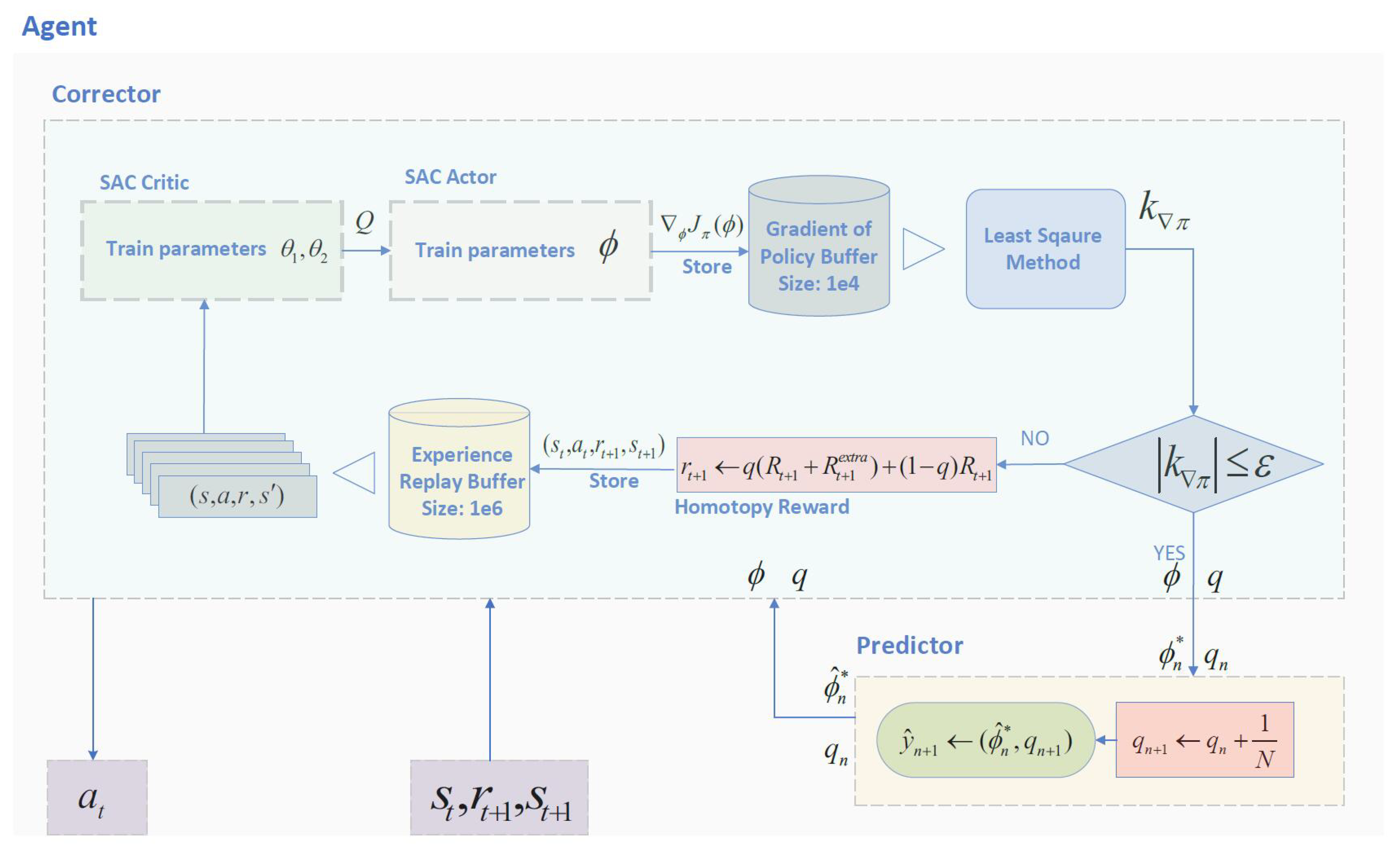
Training leverages an NVIDIA GeForce GTX 2080TI graphics card with PyTorch acceleration. The framework for the HSAC algorithm utilized by the agent is depicted in
Figure 7. The model parameters for the air combat game, as discussed in
Section 2.1 and
Section 2.2, along with the hyperparameters for the HSAC algorithm, are detailed in
Table A1 and
Table A2, respectively.
5.2. Attacking Horizontal-Flight UCAV
5.2.1. Task Setting
This experiment is designed to compare the convergence rates of different methods in a straightforward task setup. In this task, maintains a horizontal flight path at a random starting position and heading, while , controlled by the trained agent, attempts to execute an attack.
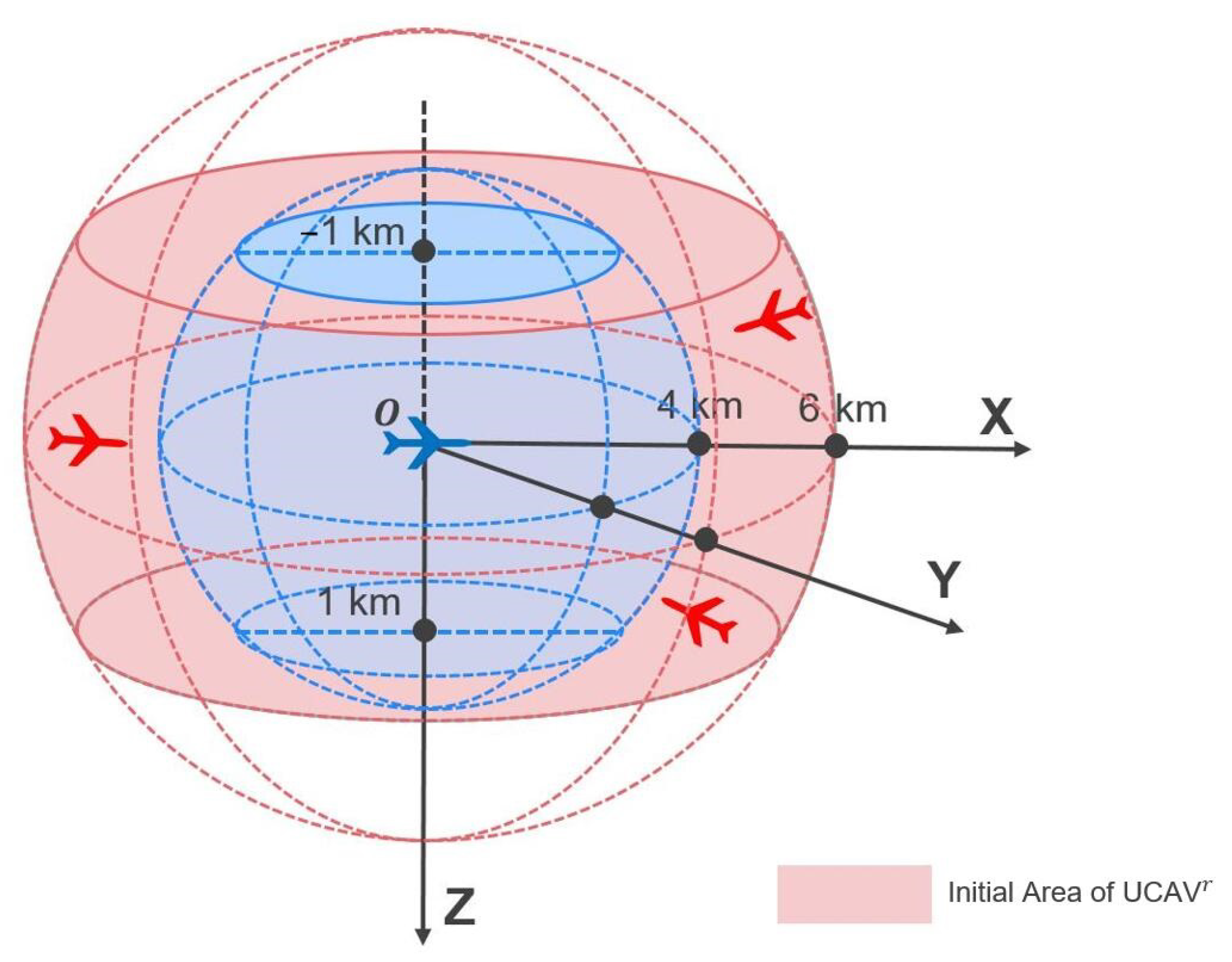
The starting point for
is designated as point
o in
Figure 8, positioned at a height of 5 km, and aligned with the
X axis with an initial heading angle of zero. The initial positioning for
is within a predefined area, as depicted in
Figure 8, with the initial relative distance ranging from 4 km to 6 km and the relative height from −1 km to 1 km. The initial heading angle for the red UCAV varies randomly from
to
.
5.2.2. Training Process
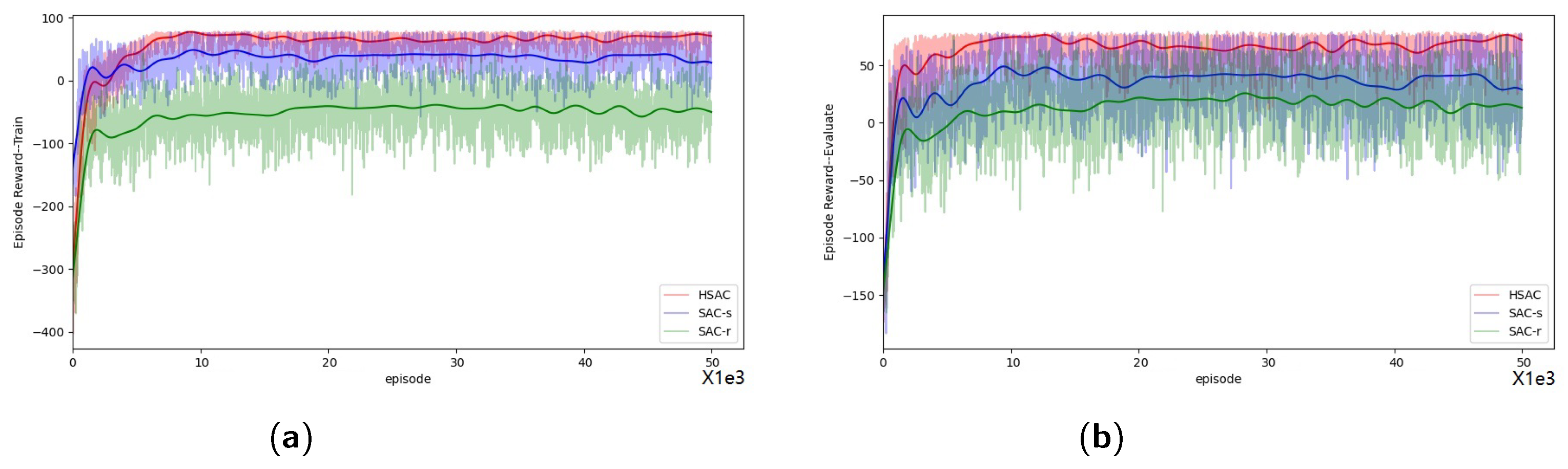
To test the convergence of the methods and the performance in the original problem, We analyze from two perspectives: the training process and the evaluation process. During the training process, the episode reward comprises both the original reward R and additional rewards such as and . In contrast, during the evaluation process, only the original reward R is considered. We periodically evaluate the quality of the policy every ten training episodes.
The models are trained for
episodes as illustrated in
Figure 9. Changes in episode rewards for different methods during the training process are displayed in
Figure 9a, and those during the evaluation process are presented in
Figure 9b.
As shown in
Figure 9a, the episode rewards during the training process generally rise with iteration, indicating that agents trained by different methods are progressively mastering the task. Notably, the agent trained with SAC-r records the lowest episode rewards, which is attributable to the negative design of
.
To gauge the training quality of each agent, attention must be directed to
Figure 9b. Here, it is evident that the agent employing HSAC achieves the highest episode rewards compared to those trained by SAC-s and SAC-r.
Although in SAC-r is crafted using artificial priors, the agent trained with SAC-r still attains lower episode rewards than the agent trained with SAC-s. Conversely, our HSAC method, using the same artificial priors, outperforms both SAC-s and SAC-r. This demonstrates that HSAC is not adversely affected by the negative aspects of artificial priors and can effectively leverage them to address the challenges posed by sparse reward RL problems with the aid of .
Subsequent analyses will compare the performance of agents trained by these methods in various air combat game scenarios post-training.
5.2.3. Simulation Results
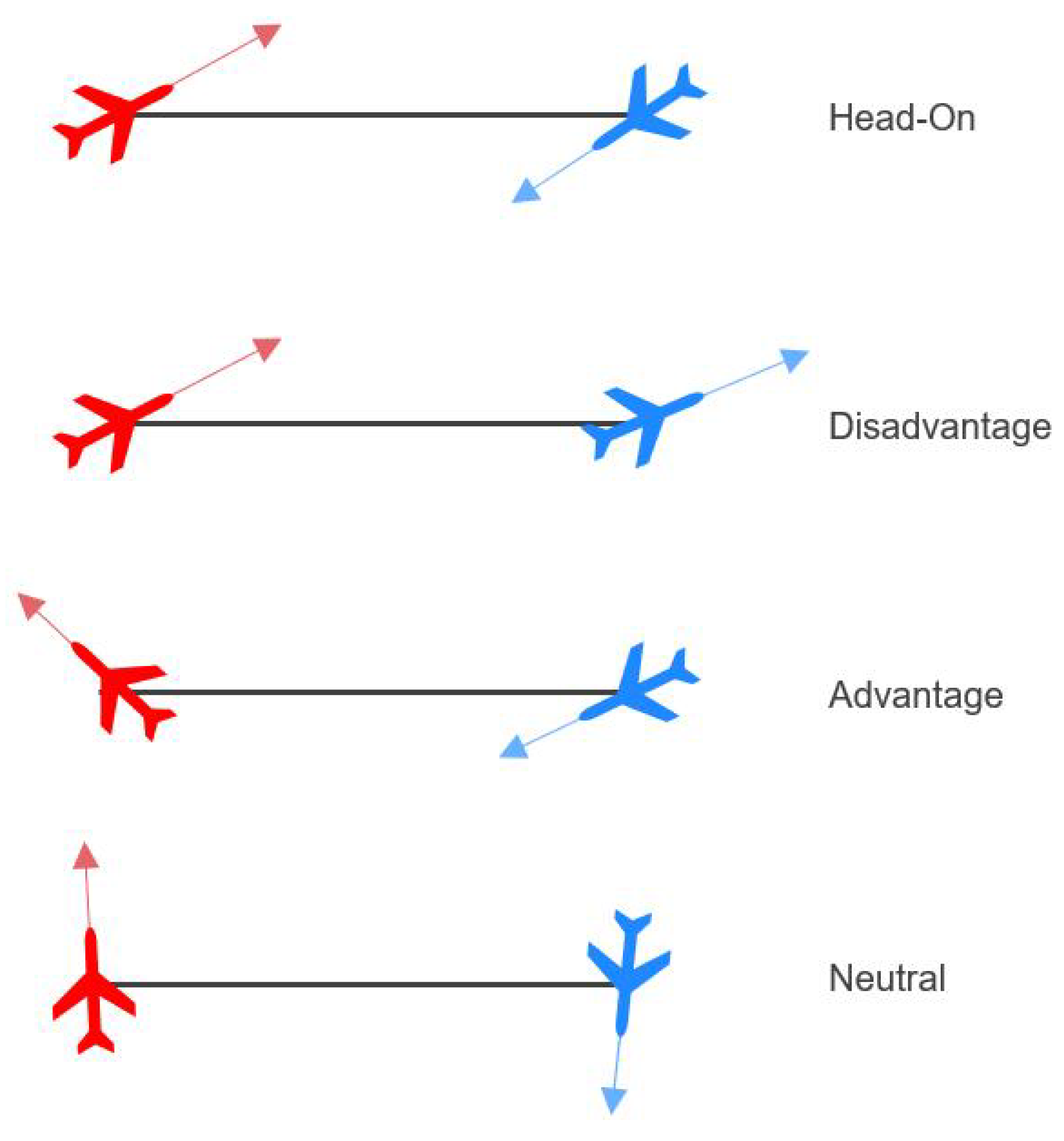
The initial state space of air combat game geometry can be divided into four categories [
24] from the perspective of
: head-on, neutral, disadvantageous, and advantageous, as illustrated in
Figure 10. Depending on these initial conditions, the win probability for
varies significantly. For instance,
is more likely to win in an advantageous position, while the odds are reversed in a disadvantageous scenario. In neutral and head-on scenarios, the win probabilities for both sides are similar. We evaluate the performance of each well-trained agent across these diverse initial scenarios.
We selected four representative initial states from each category, detailed in
Table A3. The initial bank angle
and path angle
for both
and
are set to zero. The performance metrics, including the win rates and average time cost per episode for the agents trained by different methods, are captured in
Figure 11 and
Table 1.
As illustrated in
Table 1, agents trained by SAC-s, SAC-r, and HSAC can successfully complete the task when starting from an advantageous position. The agent using SAC-r achieves this task faster than others in advantageous situations. However, in disadvantageous and head-on initial scenarios, the agent trained by HSAC significantly outperforms the others, with the highest success rates. In a disadvantageous scenario, the agent trained by SAC-s has only a
success rate, while the agent trained by SAC-r fails to succeed at all. In contrast, in head-on scenarios, while the agent trained by SAC-s has a
success rate, the one trained by SAC-r only achieves
. Although both the SAC-s and HSAC-trained agents show equal winning rates in neutral scenarios, the HSAC-trained agent completes the task more quickly.
In summary, while SAC-s fairly represents the original task, it struggles with sparse reward issues. SAC-r performs well only in advantageous scenarios due to the bias introduced by the extra rewards. However, HSAC excels in all tested scenarios, outperforming SAC-s and SAC-r by a substantial margin. HSAC effectively harnesses artificial priors without being negatively impacted by them, demonstrating its robustness across varying initial air combat game scenarios.
5.3. Self-Play Training and Two-UCAVs Game Task
5.3.1. Two-UCAVs Game Task Setting
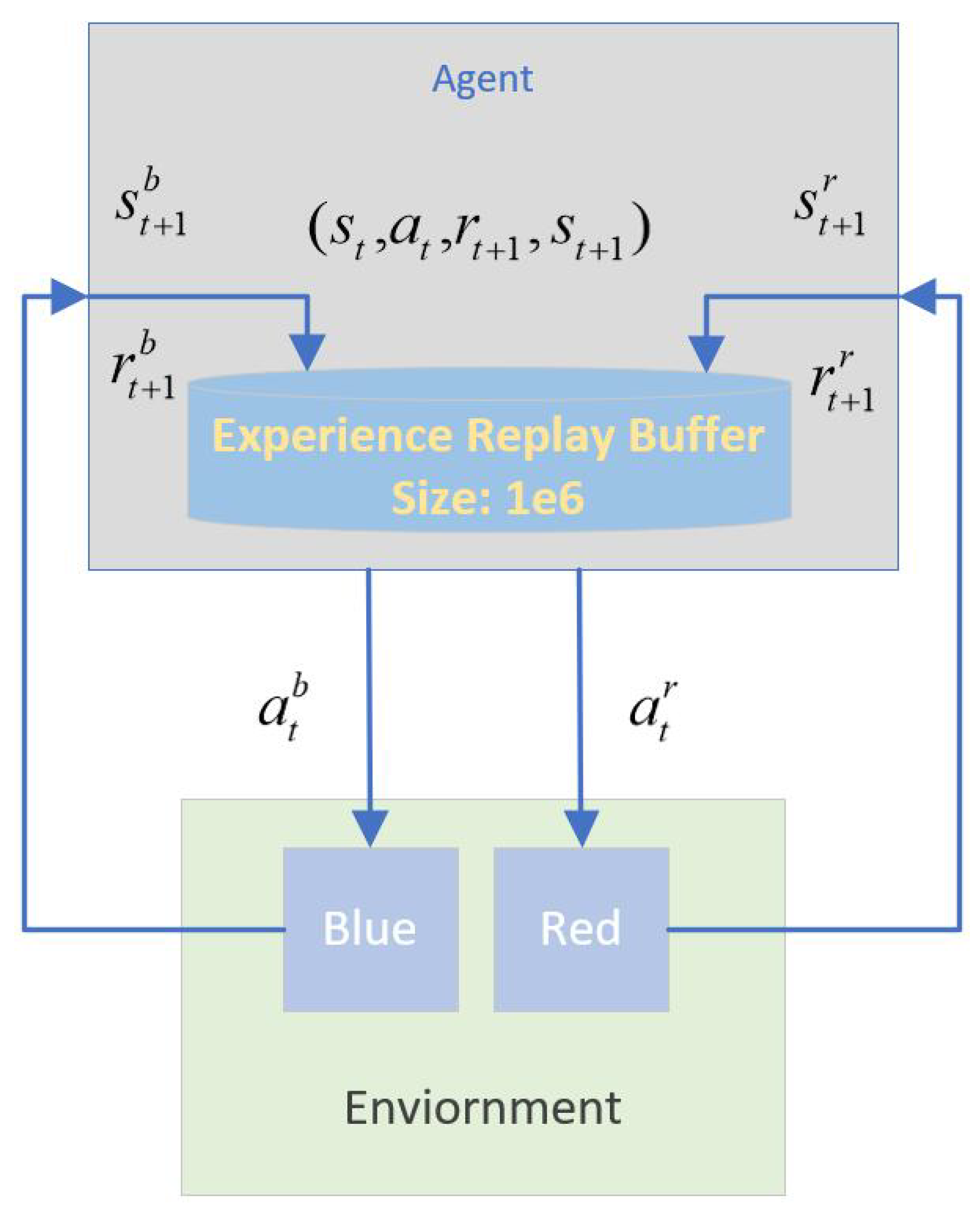
This experiment aims to demonstrate the effectiveness of the HSAC method combined with self-play in the two-UCAVs game task. Integrating self-play with HSAC, as described in
Section 4.4, allows for the development of a more sophisticated UCAV policy under air combat game conditions, optimizing the policy through competitive interactions with itself.
Figure 12 illustrates the self-play training setup, where both
and
share the same actor and critic networks. Furthermore, they share the experience replay buffer and the gradient of the policy buffer, which is essential for HSAC. The initial setup follows the parameters of the attacking horizontal-flight UCAV task outlined in
Section 5.2.1. To enhance the realism of radar detection, we set the initial line-of-sight angle component for
in the
plane between
and
. While this setup gives
an initial advantage, it serves to test if the policy can converge to an equilibrium point within the policy space, ideally demonstrating balanced offensive and defensive capabilities from any starting position.
Following the training, the performance of agents trained by SAC-s, SAC-r, and HSAC will be compared in direct confrontations.
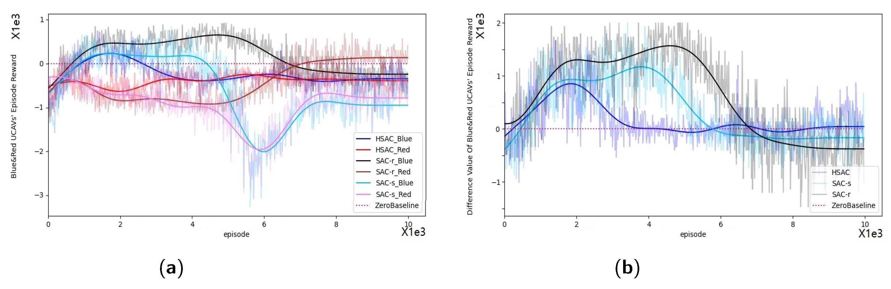
5.3.2. Training Process
The training processes for SAC-s, SAC-r, and HSAC are depicted in
Figure 13 after
training episodes. Variations in episode rewards for
and
during the self-play training are illustrated in
Figure 13a. The difference in episode rewards between
and
throughout the training process is shown in
Figure 13b. Additionally, we record the number of episodes required for method convergence, the rewards upon convergence of both
and
, and the difference in these rewards, as summarized in
Table 2, using the criteria set forth in Algorithm 2 for convergence determination.
The data in
Table 2 and
Figure 13 highlight the minimal difference in rewards upon convergence, suggesting that the policy developed through HSAC aligns closely with an equilibrium point, in accordance with Nash’s theories [
52], particularly when this difference approaches zero. This outcome underscores the efficacy of HSAC in rapidly achieving the policy that performs robustly in both offensive and defensive scenarios, as evidenced by the lowest convergence episode cost and the smallest reward discrepancies.
Post-training analysis reveals that HSAC not only converges to an equilibrium point more effectively than the other methods but also does so with superior performance consistency between the competing agents. We will next examine whether the policy honed through HSAC training outperforms those trained via other methods in subsequent head-to-head tests.
5.3.3. Simulation Results
We assess the performance of HSAC through 1 vs. 1 games played among agents trained by SAC-s, SAC-r, and HSAC. Each agent alternates between playing on the red side and the blue side over
games. The winning rates are detailed in
Table 3, with DN representing the number of draws.
Table 3 shows that when
and
operate under the same policy, players trained by SAC-r seldom achieve draws, likely due to the disproportionate reward structures which favor aggressive tactics over balanced strategic play. This undermines their ability to perform defensively, rendering SAC-r less suited for self-play training.
In contrast, the HSAC-trained agents demonstrate almost equal win rates in head-to-head matchups, reflecting robust performance across both aggressive and defensive scenarios. Notably, HSAC consistently outperforms the other methods, showcasing superior adaptability and strategic depth.
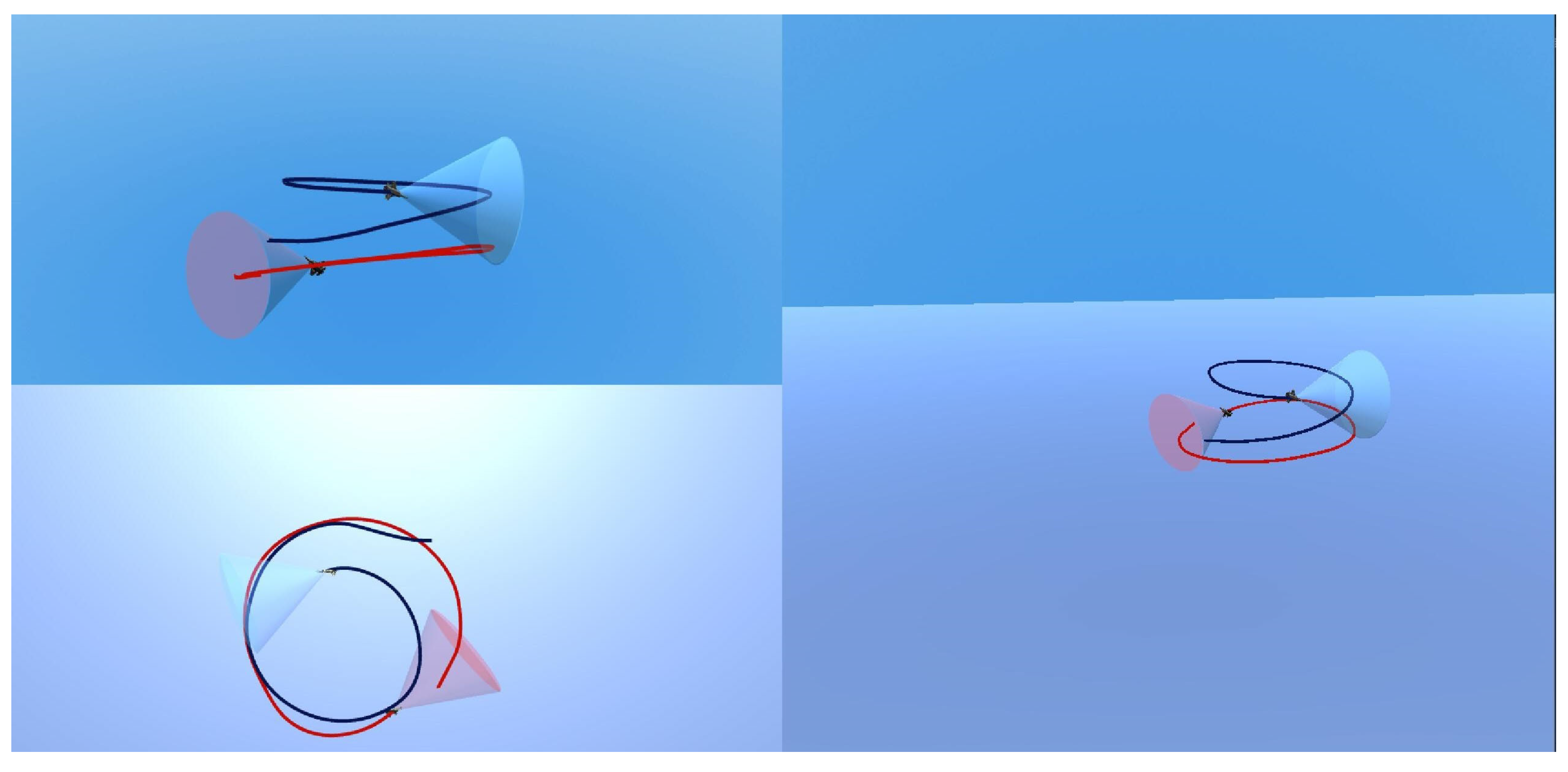
Figure 14 depicts these interactions, demonstrating how HSAC-trained agents often reach equilibrium states, effectively balancing aggressive and defensive strategies.
In summary, while SAC-s often struggles with the sparse reward problem, leading to protracted exploratory phases and suboptimal local convergence, SAC-r tends to skew learning due to its reward design. HSAC, on the other hand, utilizes homotopic techniques to smoothly transition from exploratory to optimal strategies, effectively navigating the sparse reward landscape without deviating from the task’s objectives.
6. Conclusions
In this study, we introduced the HSAC method, a novel reinforcement learning approach specifically designed to tackle the challenges associated with sparse rewards in complex RL tasks such as those found in air combat game simulations. The HSAC method begins by integrating artificial reward priors to enhance exploration efficiency, allowing for the rapid development of an initial feasible policy. As training progresses, these artificial rewards are gradually reduced to ensure that the learning process remains focused on achieving the primary objectives, thus following a homotopic path toward the optimal policy.
The results of our experiments, conducted within a sophisticated 3D simulation environment that accurately models both offensive and defensive maneuvers, demonstrate that agents trained with HSAC significantly outperform those trained using the SAC-s and SAC-r methods. Specifically, HSAC-trained agents exhibit superior combat skills and achieve higher success rates, highlighting the algorithm’s ability to effectively balance exploration and exploitation in sparse reward settings.
HSAC not only accelerates the convergence process by efficiently navigating the sparse reward landscape but also maintains robustness across various initial conditions and scenarios. This adaptability is particularly evident in our self-play experiments, where HSAC consistently achieves near-equilibrium strategies, showcasing its potential for both competitive and cooperative multi-agent environments.
Looking forward, we plan to extend the application of HSAC to multi-agent systems, further enhancing its capabilities in complex, dynamic environments. By doing so, we aim to improve its proficiency in both competitive and cooperative contexts, paving the way for broader applications in real-world scenarios.
Author Contributions
Conceptualization, Z.F., Y.Z. (Yiwen Zhu) and Y.Z. (Yuan Zheng); methodology, Y.Z. (Yiwen Zhu); software, Y.Z. (Yiwen Zhu); validation, Y.Z. (Yuan Zheng) and W.W.; formal analysis, Y.Z. (Yuan Zheng) and Y.Z. (Yiwen Zhu); investigation, Y.Z. (Yiwen Zhu); resources, Z.F.; data curation, Y.Z. (Yiwen Zhu); writing—original draft preparation, Y.Z. (Yiwen Zhu); writing—review and editing, Y.Z. (Yuan Zheng) and Z.F.; visualization, Y.Z. (Yiwen Zhu); supervision, Z.F.; project administration, Z.F. All authors have read and agreed to the published version of the manuscript.
Funding
This research was supported by the National Natural Science Foundation of China (No. U2333214).
Data Availability Statement
Data available on request from the authors.
DURC Statement
Current research is limited to the Intelligent Decision Making for Drones, which is beneficial for the further enhancement of agent intelligence and does not pose a threat to public health or national security. The authors acknowledge the dual-use potential of the research involving Intelligent Decision Making for Drones and confirm that all necessary precautions have been taken to prevent potential misuse. As an ethical responsibility, authors strictly adhere to relevant national and international laws about DURC. Authors advocate for responsible deployment, ethical considerations, regulatory compliance, and transparent reporting to mitigate misuse risks and foster beneficial outcomes.
Acknowledgments
We would like to express our sincere gratitude to Zheng Chen from the Institute of Unmanned Aerial Vehicles at Zhejiang University for his invaluable guidance and support. We are also grateful for the technical and equipment support provided by the Institute. Furthermore, we would like to thank the China Scholarship Council for their financial support during the course of this work.
Conflicts of Interest
The authors declare no conflicts of interest.
Appendix A. Proof of the Equation F3 (·)
The equation of
can be expanded as shown in Equation (
A1).
The homotopy NLP problem mentioned in
NLP3 can be described as follow:
Appendix B. Homotopic Path Existence and Convergence of the Path Following Method
Appendix B.1. Formalize the Problem as H(·) = 0
The
s in the NLP problem of
, in
Appendix A, can also be described by a state transition function
:
which means that the state
s only relates to the initial state
, time step
t, and the parameter of the policy
. Here, we use an unknown operator
to describe this relationship.
Furthermore, we can also prove the function
only relates to parameter
and
q, as shown in Equation (
A4)
Here, we use the operator to describe the relationship between the expectation of accumulated homotopic reward with the parameter and q.
Then using the Karush–Kuhn–Tucker (KKT) equations [
53] to formalize the problem described in Equation (
A2) as Equation (
A5)
Here,
is called the homotopy function. And
because
,
,
, and
. We let
and
, these and
here are only the auxiliary variables. Hence, the problem mentioned in
NLP3 is equivalent to solving the KKT equation
.
Appendix B.2. Existence of Homotopy Path
The idea of the homotopy method is to follow a path to a solution, where the “path” indicates a piecewise differentiable curve in solution space.
Zangwill [
50] defined the set of all solutions as
.
Definition A1. Given a homotopy function , we must now be more explicit about solutions toIn particular, defineas the set of all solutions The implicit function theorem can ensure that
consists solely of paths [
50]. The Jacobian of homotopy function
can be written as an
matrix, as shown in Equation (
A8).
Then, the existence of the path was given in [
50]:
Theorem A1 (Path Existence ([
50]))
. Let be continuously differentiable and suppose that for every , the Jacobian is of full rank. Then, consists only of continuously differentiable paths. As the other scholars did in homotopy optimization [
50], we give an assumption of the Jacobian matrix
:
Assumption A1. is of full rank for all .
Combining the Assumption A1 and Theorem A1, the existence of the homotopic path in this problem can be assured.
Appendix B.3. Convergence of Path Following Method
The homotopic path existence has been proved in
Appendix B.2. And then we will give the proof of the convergence and the feasibility of the path following method. In this paper, the corrector-predictor method, with horizontal corrector and elevator predictor, is used to follow the homotopic path along with the iterations. To ensure the convergence and the feasibility of this corrector-predictor path-following method, we quote Theorem A2 proposed by Zangwill [
50].
Theorem A2 (Method Convergence). For a homotopy at any , let be of full rank. Also, for , let the path be of finite length. Now, suppose that a predictor–corrector method uses the horizontal corrector and the elevator predictor.
Given sufficiently small, if for all iterations k the predictor step length is sufficiently small, then the method will follow the entire path length to any degree of accuracy.
In the traditional predictor-corrector method [
50], Equations (
A9) and (A10) are used to decide if the solution satisfies the accuracy requirement in the predictor and corrector step.
In this paper, we suppose
to be convenient to calculate.
Through Theorem A2, we can guarantee the convergence and the feasibility of using HSAC in the original problem (NLP1), with the help of the function .
Appendix C. Parameters
The hyperparameters of the HSAC algorithm, which we mentioned in
Section 4.3, are given in
Table A2.
In
Table A3, we gave four typical initial states, which were used to evaluate the quality of the policy trained by different methods in the attacking horizontal-flight UCAV task.
Table A1.
Air combat game simulation parameters.
Table A1.
Air combat game simulation parameters.
| Single UCAV Parameter | Value |
|---|
| Mass of UCAV | 150 kg |
| Max Load Factor ( | 10 g |
| Velocity Band | m/s |
| Height Range | m |
| Max Thrust ( | 100 kg |
| Range of | deg/s |
| Range of | deg/s |
| Range of | deg |
| Game Parameter | Value |
| Optimum Attack Range | (200, 2000) m |
| Maximum Iteration Step | 2000 |
Table A2.
Hyperparameters of HSAC.
Table A2.
Hyperparameters of HSAC.
| Parameter | Value |
|---|
| Optimizer | Adam |
| Learning Rate | |
| Discount () | 0.996 |
| Number of Hidden Layers (All Networks) | 3 |
| Number of Hidden Units per Layer | 256 |
| Number of Samples per Minibatch | 256 |
| Nonlinearity | ReLU |
| Replay Buffer size | |
| Entropy Target | −dim(A) |
| Target Smoothing Coefficient () | 0.005 |
| Policy Gradient Buffer (M) | |
| Total Number of Homotopy Iterations (N) | 100 |
| Threshold of () | |
Table A3.
Initial state settings for evaluating the quality of agents.
Table A3.
Initial state settings for evaluating the quality of agents.
| Initial State | | | | | |
|---|
| Advantageous | Blue | 0 | 0 | 5000 | 150 | 45 |
| Red | 5000 | 5000 | 5000 | 150 | 45 |
| Disadvantageous | Blue | 0 | 0 | 5000 | 150 | −45 |
| Red | −5000 | 5000 | 5000 | 150 | −45 |
| Head-On | Blue | 0 | 0 | 5000 | 150 | 45 |
| Red | 5000 | 5000 | 5000 | 150 | −135 |
| Neutral | Blue | 0 | 0 | 5000 | 150 | 45 |
| Red | 5000 | −5000 | 5000 | 150 | −135 |
References
- Xu, G.; Wei, S.; Zhang, H. Application of situation function in air combat differential games. In Proceedings of the 2017 36th Chinese Control Conference (CCC), Dalian, China, 26–28 July 2017; IEEE: Piscataway, NJ, USA, 2017; pp. 5865–5870. [Google Scholar]
- Park, H.; Lee, B.Y.; Tahk, M.J.; Yoo, D.W. Differential game based air combat maneuver generation using scoring function matrix. Int. J. Aeronaut. Space Sci. 2016, 17, 204–213. [Google Scholar] [CrossRef]
- Virtanen, K.; Karelahti, J.; Raivio, T. Modeling air combat by a moving horizon influence diagram game. J. Guid. Control Dyn. 2006, 29, 1080–1091. [Google Scholar] [CrossRef]
- Zhong, L.; Tong, M.; Zhong, W.; Zhang, S. Sequential maneuvering decisions based on multi-stage influence diagram in air combat. J. Syst. Eng. Electron. 2007, 18, 551–555. [Google Scholar]
- Ortiz, A.; Garcia-Nieto, S.; Simarro, R. Comparative Study of Optimal Multivariable LQR and MPC Controllers for Unmanned Combat Air Systems in Trajectory Tracking. Electronics 2021, 10, 331. [Google Scholar] [CrossRef]
- Smith, R.E.; Dike, B.; Mehra, R.; Ravichandran, B.; El-Fallah, A. Classifier systems in combat: Two-sided learning of maneuvers for advanced fighter aircraft. Comput. Methods Appl. Mech. Eng. 2000, 186, 421–437. [Google Scholar] [CrossRef]
- Changqiang, H.; Kangsheng, D.; Hanqiao, H.; Shangqin, T.; Zhuoran, Z. Autonomous air combat maneuver decision using Bayesian inference and moving horizon optimization. J. Syst. Eng. Electron. 2018, 29, 86–97. [Google Scholar]
- Shenyu, G. Research on Expert System and Decision Support System for Multiple Air Combat Tactical Maneuvering. Syst. Eng.-Theory Pract. 1999, 8, 76–80. [Google Scholar]
- Zhao, W.; Zhou, D.Y. Application of expert system in sequencing of air combat multi-target attacking. Electron. Opt. Control 2008, 2, 23–26. [Google Scholar]
- Bechtel, R.J. Air Combat Maneuvering Expert System Trainer; Technical Report; Merit Technology Inc.: Plano, TX, USA, 1992. [Google Scholar]
- Xu, J.; Zhang, J.; Yang, L.; Liu, C. Autonomous decision-making for dogfights based on a tactical pursuit point approach. Aerosp. Sci. Technol. 2022, 129, 107857. [Google Scholar] [CrossRef]
- Rodin, E.Y.; Amin, S.M. Maneuver prediction in air combat via artificial neural networks. Comput. Math. Appl. 1992, 24, 95–112. [Google Scholar] [CrossRef]
- Schvaneveldt, R.W.; Goldsmith, T.E.; Benson, A.E.; Waag, W.L. Neural Network Models of Air Combat Maneuvering; Technical Report; New Mexico State University: Las Cruces, NM, USA, 1992. [Google Scholar]
- Teng, T.H.; Tan, A.H.; Tan, Y.S.; Yeo, A. Self-organizing neural networks for learning air combat maneuvers. In Proceedings of the 2012 International Joint Conference on Neural Networks (IJCNN), Brisbane, Australia, 10–15 June 2012; IEEE: Piscataway, NJ, USA, 2012; pp. 1–8. [Google Scholar]
- Sutton, R.S.; Barto, A.G. Reinforcement Learning: An Introduction; MIT Press: Cambridge, MA, USA, 2018. [Google Scholar]
- Ding, Y.; Kuang, M.; Shi, H.; Gao, J. Multi-UAV Cooperative Target Assignment Method Based on Reinforcement Learning. Drones 2024, 8, 562. [Google Scholar] [CrossRef]
- Yang, J.; Yang, X.; Yu, T. Multi-Unmanned Aerial Vehicle Confrontation in Intelligent Air Combat: A Multi-Agent Deep Reinforcement Learning Approach. Drones 2024, 8, 382. [Google Scholar] [CrossRef]
- Gao, X.; Zhang, Y.; Wang, B.; Leng, Z.; Hou, Z. The Optimal Strategies of Maneuver Decision in Air Combat of UCAV Based on the Improved TD3 Algorithm. Drones 2024, 8, 501. [Google Scholar] [CrossRef]
- Guo, J.; Zhang, J.; Wang, Z.; Liu, X.; Zhou, S.; Shi, G.; Shi, Z. Formation Cooperative Intelligent Tactical Decision Making Based on Bayesian Network Model. Drones 2024, 8, 427. [Google Scholar] [CrossRef]
- Chen, C.L.; Huang, Y.W.; Shen, T.J. Application of Deep Reinforcement Learning to Defense and Intrusion Strategies Using Unmanned Aerial Vehicles in a Versus Game. Drones 2024, 8, 365. [Google Scholar] [CrossRef]
- McGrew, J.S.; How, J.P.; Williams, B.; Roy, N. Air-combat strategy using approximate dynamic programming. J. Guid. Control Dyn. 2010, 33, 1641–1654. [Google Scholar] [CrossRef]
- Crumpacker, J.B.; Robbins, M.J.; Jenkins, P.R. An approximate dynamic programming approach for solving an air combat maneuvering problem. Expert Syst. Appl. 2022, 203, 117448. [Google Scholar] [CrossRef]
- Ma, X.; Xia, L.; Zhao, Q. Air-combat strategy using Deep Q-Learning. In Proceedings of the 2018 Chinese Automation Congress (CAC), Xi’an, China, 30 November–2 December 2018; IEEE: Piscataway, NJ, USA, 2018; pp. 3952–3957. [Google Scholar]
- Wang, Z.; Li, H.; Wu, H.; Wu, Z. Improving maneuver strategy in air combat by alternate freeze games with a deep reinforcement learning algorithm. Math. Probl. Eng. 2020, 2020, 7180639. [Google Scholar] [CrossRef]
- Yang, Q.; Zhang, J.; Shi, G.; Hu, J.; Wu, Y. Maneuver decision of UAV in short-range air combat based on deep reinforcement learning. IEEE Access 2019, 8, 363–378. [Google Scholar] [CrossRef]
- Pope, A.P.; Ide, J.S.; Mićović, D.; Diaz, H.; Rosenbluth, D.; Ritholtz, L.; Twedt, J.C.; Walker, T.T.; Alcedo, K.; Javorsek, D. Hierarchical Reinforcement Learning for Air-to-Air Combat. In Proceedings of the 2021 International Conference on Unmanned Aircraft Systems (ICUAS), Athens, Greece, 15–18 June 2021; pp. 275–284. [Google Scholar] [CrossRef]
- Ng, A.Y.; Harada, D.; Russell, S. Policy invariance under reward transformations: Theory and application to reward shaping. In Proceedings of the Sixteenth International Conference on Machine Learning (ICML 1999), Bled, Slovenia, 27–30 June 1999; Volume 99, pp. 278–287. [Google Scholar]
- Randløv, J.; Alstrøm, P. Learning to Drive a Bicycle Using Reinforcement Learning and Shaping. In Proceedings of the ICML, San Francisco, CA, USA, 24–27 July 1998; Citeseer: Princeton, NJ, USA, 1998; Volume 98, pp. 463–471. [Google Scholar]
- Gu, S.; Holly, E.; Lillicrap, T.; Levine, S. Deep reinforcement learning for robotic manipulation with asynchronous off-policy updates. In Proceedings of the 2017 IEEE International Conference on Robotics and Automation (ICRA), Singapore, 29 May–3 June 2017; IEEE: Piscataway, NJ, USA, 2017; pp. 3389–3396. [Google Scholar]
- Heess, N.; TB, D.; Sriram, S.; Lemmon, J.; Merel, J.; Wayne, G.; Tassa, Y.; Erez, T.; Wang, Z.; Eslami, S.; et al. Emergence of locomotion behaviours in rich environments. arXiv 2017, arXiv:1707.02286. [Google Scholar]
- Ghosh, D.; Singh, A.; Rajeswaran, A.; Kumar, V.; Levine, S. Divide-and-conquer reinforcement learning. arXiv 2017, arXiv:1711.09874. [Google Scholar]
- Forestier, S.; Portelas, R.; Mollard, Y.; Oudeyer, P.Y. Intrinsically motivated goal exploration processes with automatic curriculum learning. arXiv 2017, arXiv:1708.02190. [Google Scholar]
- Ross, S.; Gordon, G.; Bagnell, D. A reduction of imitation learning and structured prediction to no-regret online learning. In Proceedings of the Fourteenth International Conference on Artificial Intelligence and Statistics, Fort Lauderdale, FL, USA, 11–13 April 2011; pp. 627–635. [Google Scholar]
- Vecerik, M.; Hester, T.; Scholz, J.; Wang, F.; Pietquin, O.; Piot, B.; Heess, N.; Rothörl, T.; Lampe, T.; Riedmiller, M. Leveraging demonstrations for deep reinforcement learning on robotics problems with sparse rewards. arXiv 2017, arXiv:1707.08817. [Google Scholar]
- Kober, J.; Peters, J. Policy search for motor primitives in robotics. Mach. Learn. 2011, 84, 171–203. [Google Scholar] [CrossRef]
- Montgomery, W.H.; Levine, S. Guided policy search via approximate mirror descent. Adv. Neural Inf. Process. Syst. 2016, 29, 4008–4016. [Google Scholar]
- Ziebart, B.D.; Maas, A.L.; Bagnell, J.A.; Dey, A.K. Maximum entropy inverse reinforcement learning. In Proceedings of the AAAI, Chicago, IL, USA, 13–17 July 2008; Volume 8, pp. 1433–1438. [Google Scholar]
- Shaw, R.L. Fighter Combat. Tactics and Maneuvering; Naval Institute Press: Annapolis, MD, USA, 1985. [Google Scholar]
- Grimm, W.; Well, K. Modelling air combat as differential game recent approaches and future requirements. In Differential Games—Developments in Modelling and Computation, Proceedings of the Fourth International Symposium on Differential Games and Applications, Otaniemi, Finland, 9–10 August 1990; Springer: Berlin/Heidelberg, Germany, 1991; pp. 1–13. [Google Scholar]
- Blaquière, A.; Gérard, F.; Leitmann, G. Quantitative and Qualitative Games by Austin Blaquiere, Francoise Gerard and George Leitmann; Academic Press: Cambridge, MA, USA, 1969. [Google Scholar]
- Silver, D.; Hubert, T.; Schrittwieser, J.; Antonoglou, I.; Lai, M.; Guez, A.; Lanctot, M.; Sifre, L.; Kumaran, D.; Graepel, T.; et al. A general reinforcement learning algorithm that masters chess, shogi, and Go through self-play. Science 2018, 362, 1140–1144. [Google Scholar] [CrossRef]
- Haarnoja, T.; Zhou, A.; Abbeel, P.; Levine, S. Soft actor-critic: Off-policy maximum entropy deep reinforcement learning with a stochastic actor. In Proceedings of the International Conference on Machine Learning. PMLR, Stockholm, Sweden, 10–15 July 2018; pp. 1861–1870. [Google Scholar]
- Ziebart, B.D. Modeling Purposeful Adaptive Behavior with the Principle of Maximum Causal Entropy; Carnegie Mellon University: Pittsburgh, PA, USA, 2010. [Google Scholar]
- Haarnoja, T.; Tang, H.; Abbeel, P.; Levine, S. Reinforcement learning with deep energy-based policies. In Proceedings of the International Conference on Machine Learning, PMLR, Sydney, Australia, 6–11 August 2017; pp. 1352–1361. [Google Scholar]
- Fujimoto, S.; Hoof, H.; Meger, D. Addressing function approximation error in actor-critic methods. In Proceedings of the International Conference on Machine Learning, PMLR, Stockholm, Sweden, 10–15 July 2018; pp. 1587–1596. [Google Scholar]
- Haarnoja, T.; Zhou, A.; Hartikainen, K.; Tucker, G.; Ha, S.; Tan, J.; Kumar, V.; Zhu, H.; Gupta, A.; Abbeel, P.; et al. Soft actor-critic algorithms and applications. arXiv 2018, arXiv:1812.05905. [Google Scholar]
- Kong, W.; Zhou, D.; Yang, Z.; Zhao, Y.; Zhang, K. Uav autonomous aerial combat maneuver strategy generation with observation error based on state-adversarial deep deterministic policy gradient and inverse reinforcement learning. Electronics 2020, 9, 1121. [Google Scholar] [CrossRef]
- Forsythe, G.E. Computer Methods for Mathematical Computations; Prentice Hall: Upper Saddle River, NJ, USA, 1977. [Google Scholar]
- Bertsekas, D. Reinforcement Learning and Optimal Control; Athena Scientific: Nashua, NH, USA, 2019. [Google Scholar]
- Lemke, C. Pathways to solutions, fixed points, and equilibria (cb garcia and wj zangwill). Sch. J. 1984, 26, 445. [Google Scholar]
- Brockman, G.; Cheung, V.; Pettersson, L.; Schneider, J.; Schulman, J.; Tang, J.; Zaremba, W. OpenAI Gym. arXiv 2016, arXiv:1606.01540. [Google Scholar]
- Nash, J. Non-cooperative games. Ann. Math. 1951, 54, 286–295. [Google Scholar] [CrossRef]
- Fiacco, A.V.; McCormick, G.P. Nonlinear Programming: Sequential Unconstrained Minimization Techniques; Society for Industrial and Applied Mathematics: Philadelphia, PA, USA, 1990. [Google Scholar]
Figure 1.
Overview diagram of HSAC in the air combat game environment.
Figure 1.
Overview diagram of HSAC in the air combat game environment.
Figure 2.
One-to-one short-range air combat game scenario.
Figure 2.
One-to-one short-range air combat game scenario.
Figure 3.
Three-degree-of-freedom particle model of the UCAV in the ground coordinate system with dotted lines as visual aids for attitude understanding.
Figure 3.
Three-degree-of-freedom particle model of the UCAV in the ground coordinate system with dotted lines as visual aids for attitude understanding.
Figure 4.
The diagrammatic sketch of three-dimensional air combat game.
Figure 4.
The diagrammatic sketch of three-dimensional air combat game.
Figure 5.
The framework of the air combat game environment.
Figure 5.
The framework of the air combat game environment.
Figure 6.
The simulation platform established by Unity3D and Gym.The blue and red lines in the figure correspond to the flight trajectories of the aircraft.
Figure 6.
The simulation platform established by Unity3D and Gym.The blue and red lines in the figure correspond to the flight trajectories of the aircraft.
Figure 7.
The construction of the HSAC method.
Figure 7.
The construction of the HSAC method.
Figure 8.
Initial state of blue and red UCAV.
Figure 8.
Initial state of blue and red UCAV.
Figure 9.
The episode reward of different methods in attacking horizontal-flight UCAV task, the results of the training process reflect the quality of convergence, and the results of the evaluating process reflect the performance of different methods in the original problem. (a) Illustrates the episode reward in the training process. (b) Denotes the episode reward in the evaluating process.
Figure 10.
Four initial air combat game scenario categories.
Figure 10.
Four initial air combat game scenario categories.
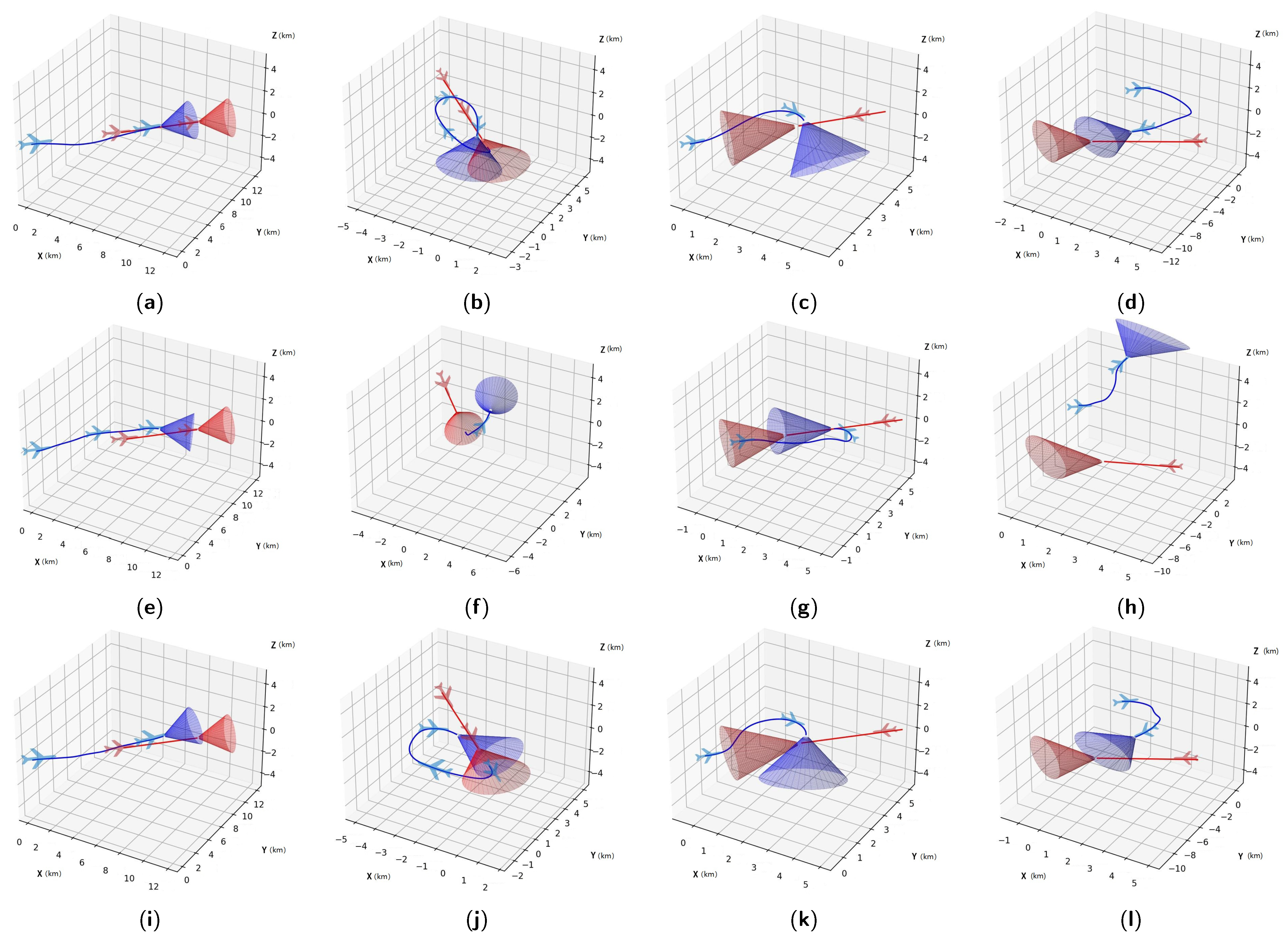
Figure 11.
Performance of agents trained by different methods with different initial situations in the attacking horizontal-flight UCAV task, where red and blue are used to conveniently distinguish between different aircraft: (a) Agent trained by SAC-s in an advantageous situation; (b) Agent trained by SAC-s in a disadvantageous situation; (c) Agent trained by SAC-s in a head-on situation; (d) Agent trained by SAC-s in a neutral situation; (e) Agent trained by SAC-r in an advantageous situation; (f) Agent trained by SAC-r in a disadvantageous situation; (g) Agent trained by SAC-r in a head-on situation; (h) Agent trained by SAC-r in a neutral situation; (i) Agent trained by HSAC in an advantageous situation; (j) Agent trained by HSAC in a disadvantageous situation; (k) Agent trained by HSAC in a head-on situation; (l) Agent trained by HSAC in a neutral situation.
Figure 12.
The structure of the two-UCAVs game task with the idea of self-play.
Figure 12.
The structure of the two-UCAVs game task with the idea of self-play.
Figure 13.
The self-play training process of SAC-s, HSAC, and SAC-r in the two-UCAVs game task: (a) Displays the episode rewards for and across different methods. (b) Shows the difference in episode rewards between and trained by different methods.
Figure 13.
The self-play training process of SAC-s, HSAC, and SAC-r in the two-UCAVs game task: (a) Displays the episode rewards for and across different methods. (b) Shows the difference in episode rewards between and trained by different methods.
Figure 14.
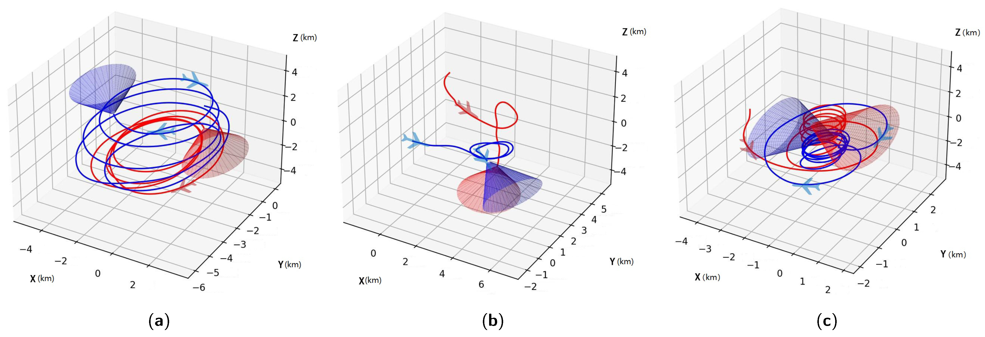
(a) HSAC-trained agent competing against SAC-s-trained agent; HSAC plays as and SAC-s as . (b) HSAC-trained agent competing against SAC-r-trained agent; HSAC plays as and SAC-r as . (c) HSAC-trained agent competes against another HSAC-trained agent, demonstrating the equilibrium strategy effectiveness. Red and blue are used to conveniently distinguish between different aircraft.
Figure 14.
(a) HSAC-trained agent competing against SAC-s-trained agent; HSAC plays as and SAC-s as . (b) HSAC-trained agent competing against SAC-r-trained agent; HSAC plays as and SAC-r as . (c) HSAC-trained agent competes against another HSAC-trained agent, demonstrating the equilibrium strategy effectiveness. Red and blue are used to conveniently distinguish between different aircraft.
Table 1.
Performance of agents trained by different methods in attacking horizontal-flight tasks with different initial states after episode evaluations.
Table 1.
Performance of agents trained by different methods in attacking horizontal-flight tasks with different initial states after episode evaluations.
| Method | SAC-s | SAC-r | HSAC |
|---|
|
Initial State | |
|---|
| Advantageous | Winning Rate | 100.00% | 100.00 % | 100.00% |
| Average Time Cost | 42.07 s | 37.90 s | 39.40 s |
| Disadvantageous | Winning Rate | | | 98.38% |
| Average Time Cost | 44.66 s | 26.23 s | 35.91 s |
| Head-On | Winning Rate | | | 99.94% |
| Average Time Cost | 39.15 s | 31.02 s | 24.73 s |
| Neutral | Winning Rate | 100.00% | | 100.00% |
| Average Time Cost | 40.05 s | 22.57 s | 33.20 s |
Table 2.
The convergence episode cost for three different methods, the episode reward of the converged policy, and the difference value of converged episode reward between and in the self-play training process.
Table 2.
The convergence episode cost for three different methods, the episode reward of the converged policy, and the difference value of converged episode reward between and in the self-play training process.
| | SAC-r | SAC-s | HSAC |
|---|
| | Blue | Red | Blue | Red | Blue | Red |
|---|
Quality
of Policy | Episode Reward | −217.64 | 111.72 | −1469.09 | −1339.13 | −387.52 | −382.57 |
| Difference Value | 329.36 | 129.96 | 4.95 |
| Convergence Episode Cost (episodes) | 8250 | 6675 | 4455 |
Table 3.
The relative winning rates of agents trained by different methods after episodes’ evaluation in two-UCAVs game task, where DN means the number of draws.
Table 3.
The relative winning rates of agents trained by different methods after episodes’ evaluation in two-UCAVs game task, where DN means the number of draws.
| Red | SAC-s | SAC-r | HSAC |
|---|
|
Blue | |
|---|
| SAC-s | Blue Win | | | |
| Red Win | | | |
| DN | 43,785 | 372 | 49,939 |
| SAC-r | Blue Win | | | |
| Red Win | | | |
| DN | 328 | 1 | 619 |
| HSAC | Blue Win | | | |
| Red Win | | | |
| DN | 35,448 | 843 | 75,228 |
| Disclaimer/Publisher’s Note: The statements, opinions and data contained in all publications are solely those of the individual author(s) and contributor(s) and not of MDPI and/or the editor(s). MDPI and/or the editor(s) disclaim responsibility for any injury to people or property resulting from any ideas, methods, instructions or products referred to in the content. |
© 2024 by the authors. Licensee MDPI, Basel, Switzerland. This article is an open access article distributed under the terms and conditions of the Creative Commons Attribution (CC BY) license (https://creativecommons.org/licenses/by/4.0/).


