An Enhanced Adaptive Ensemble Kalman Filter for Autonomous Underwater Vehicle Integrated Navigation

Abstract

Autonomous Underwater Vehicles (AUVs) rely on integrated navigation systems and corresponding filtering algorithms to ensure mission success and the spatiotemporal accuracy of sampled data. Among these, the ensemble Kalman filter (EnKF) combines Monte Carlo methods with the Kalman filter, which is particularly suited for nonlinear systems. This study proposes an enhanced adaptive EnKF algorithm to improve the smoothness and accuracy of the filtering process. Instead of the conventional Gaussian distribution, this algorithm employs a Laplace distribution to construct the system state vector and observation vector ensembles, enhancing stability against non-Gaussian noise. Additionally, the algorithm dynamically adjusts the number of vector members in the ensemble using adaptive mechanisms by specifying thresholds during filtering to adapt the requirements of real-world observational settings. Using field trial data from DVL, GPS, and electronic compass measurements, we optimize the algorithm’s parameter settings and evaluate the overall performance of the algorithm. Results indicate that the proposed adaptive EnKF achieves superior accuracy and smoothness performance. Compared to the conventional EnKF and EKF, it not only reduces the average positioning error by 30% and 44%, respectively, but also significantly improves the filtering smoothness and stability, highlighting its advantages for AUV navigation.

1. Introduction

Autonomous Underwater Vehicles (AUVs) have become indispensable in ocean exploration due to their high mobility and intelligence. Precise navigation systems are crucial for AUV operations, especially in complex underwater environments, where various disturbances can affect single-source navigation thus impacting positioning accuracy and motion stability [1]. The primary navigation methods for AUVs include dead reckoning based on inertial navigation, underwater acoustic navigation, and geophysical navigation [2]. To address the limitations of single-source navigation, AUVs commonly integrate multiple sensors such as electronic compasses, Doppler Velocity Logs (DVLs), GPS, Ultra-Short Baseline (USBL) systems, and Inertial Navigation Systems (INSs) [3]. By applying filtering algorithms, INSs fuse and optimize navigation information from multiple sources, enhancing the overall stability and accuracy of the AUV’s positioning capability [4].

In the late half of the 20th century, technological constraints, including AUV size, high power consumption, and navigation system costs, hindered widespread adoption [5]. Therefore, the related research primarily focused on the optimization of the system hardware construction and cost reduction. In the Autonomous Minehunting and Mapping Technologies Program by the U.S. Defense Advanced Research Projects Agency, a Doppler-assisted AUV navigation system integrating Doppler sonar, an inertial navigation unit, and GPS was developed [6]. This system uses an enhanced Kalman filter algorithm to optimize navigation data, achieving a positioning accuracy of nearly 0.02% of the total travel distance during testing. Larsen developed the MARPOS navigation system by integrating sensors such as Ring Laser Gyro, DVL, INS, Short Baseline, and GPS. After extensive testing, MARPOS has proven reliable and accurate, and is now applied in the Mardian line of commercial AUVs [7]. Under the impetus of the “863” project, China developed the first 6000 m-class AUV “CR-01” in 2001 [8]. The AUV’s navigation system, combining INS, DVL, and Long Baseline, maintained positioning errors within 10 m in the system’s coverage area. This enabled the AUV to successfully complete two research missions investigating manganese nodules on the Pacific Ocean floor.

Advances in technology, especially in battery capacity, now allow AUVs to perform prolonged underwater tasks, surpassing traditional manned submersibles and ROVs. However, this extended mission capability demands higher navigation precision [9]. Zhang et al. provide a comprehensive review and summary of the composition and development history of AUV navigation systems since the 1980s [10]. Currently, AUV navigation is shifting from traditional methods that require pre-deployed positioning devices, like Long Baseline and USBL, toward dynamic multi-agent systems. New techniques such as Simultaneous Localization and Mapping are significantly improving the cost-effectiveness and accuracy of AUV navigation [11].

The central issue in the field of AUV navigation is the state estimation [12]. To enhance positioning performance, research on integrated navigation systems is increasingly focused on improving nonlinear filtering algorithms. To further enhance the accuracy and stability of target tracking, recent years have witnessed extensive research on nonlinear filtering algorithms for multi-target tracking, localization, and multi-sensor data fusion in various scenarios [13,14,15]. In navigation applications, the Kalman filter (KF) is the most commonly used algorithm for handling multi-sensor data fusion [16]. The KF algorithm was often used in early AUV navigation systems to achieve the data fusion between different hardware components [17]. To better address the nonlinear system filtering problem, various different nonlinear filtering algorithms have been further developed based on the KF. The Extended Kalman Filter (EKF) is a widely used Kalman Filter variant in AUV navigation systems, which handles nonlinearity by approximating it through a first-order Taylor expansion. This makes it particularly effective for systems with mild nonlinearity and non-Gaussian characteristics, contributing to its extensive use in AUV integrated navigation systems [18]. Fulton et al. tested the EKF algorithm on the REMUS AUV by post-processing data from an acoustic navigation system, Doppler sonar, and compass [19]. Their enhanced EKF algorithm autonomously detects and removes outliers, consistently delivering stable performance with a positioning accuracy error margin within a few meters.

EKF has the advantages of easy implementation and faster operation speed. However, linearizing nonlinear terms via first-order Taylor expansion introduces errors, which can escalate or cause dispersion in filtering accuracy, especially in strongly nonlinear systems. To enhance the navigation accuracy, several studies have attempted to combine the KF with other nonlinear methods. Addressing EKF’s limitations, Crassidis proposed the Sigma Point Kalman Filter (SPKF), which optimizes the fusion of GPS and INS data [20]. Similarly, the Unscented Kalman Filter (UKF) uses the unscented transform, offering greater accuracy and simpler implementation than the EKF for nonlinear estimation [21,22]. On this basis, Krauss et al. developed a manifold-based UKF that filters out sensor measurement outliers, effectively enhancing AUV speed estimation and heading convergence [23]. In addition, the Particle filter is another popular nonlinear filtering technique, which uses Monte Carlo sampling with particle weights to represent system probability density, allowing state estimation without analytical solutions [24,25,26].

Similarly to the Particle filter, the ensemble Kalman filter (EnKF) is a nonlinear filtering algorithm that combines the KF with the Monte Carlo method, which constructs sample ensembles to replace the covariance matrix operation. Due to its great ability to handle high-dimensional nonlinear systems, the EnKF is now widely used in the field of meteorological model prediction [27]. In recent years, some studies have also applied it to the fields of navigation and control, achieving impressive results. Cui and Zhang applied the EnKF algorithm to multi-sensor target tracking, and empirical tests showed it outperformed the traditional EKF, confirming its effectiveness for AUV navigation systems [28]. Pornsarayouth et al. combined one-step smoothing with the EnKF to improve multi-sensor target positioning, and simulations showed that the EnKF outperformed the EKF and PF in handling “out-of-sequence” measurements in integrated navigation systems [29]. Tin et al. have conducted extensive research on the application of the EnKF in AUV underwater navigation [30]. They applied the KF, EnKF, and FKF independently to AUV navigation data, assessing performance by computing the runtime and the root mean square error (RMSE) of positioning data. Results showed that the EnKF outperformed FKF in both computational efficiency and 3D positioning accuracy [31]. They simulated AUV motion in 3D space to further assess the EnKF’s positioning performance across different ensemble sizes. Results showed that the EnKF maintained low average positioning errors, with accuracy improving as ensemble size increased, though at the expense of computational speed [32].

The EnKF was demonstrated to be effective in AUV integrated navigation systems, but it still has notable limitations. First, the EnKF algorithm replaces traditional covariance matrix operations with statistical analyses of randomly generated sample ensembles. The outcomes of this method are significantly influenced by the number and mathematical properties of these samples, resulting in a filter output that exhibits instable variability. In comparison to the conventional KF or EKF approaches, the EnKF exhibits less smoothness and stability in its filtering trajectory. Second, although the EnKF can effectively handle the nonlinear systems, its stability may degrade under common non-Gaussian noise disturbances in marine environments. To address these issues, improvements to the EnKF algorithm should start with the sample ensemble generation. This involves enhancing the algorithm’s stability by modifying the sample generation process and dynamically adjusting the number of samples in the ensemble. By balancing precision and efficiency, these modifications aim to optimize overall filtering performance.

This paper proposes an enhanced adaptive EnKF algorithm for AUV integrated navigation. The highlights of the enhanced algorithm include the following:

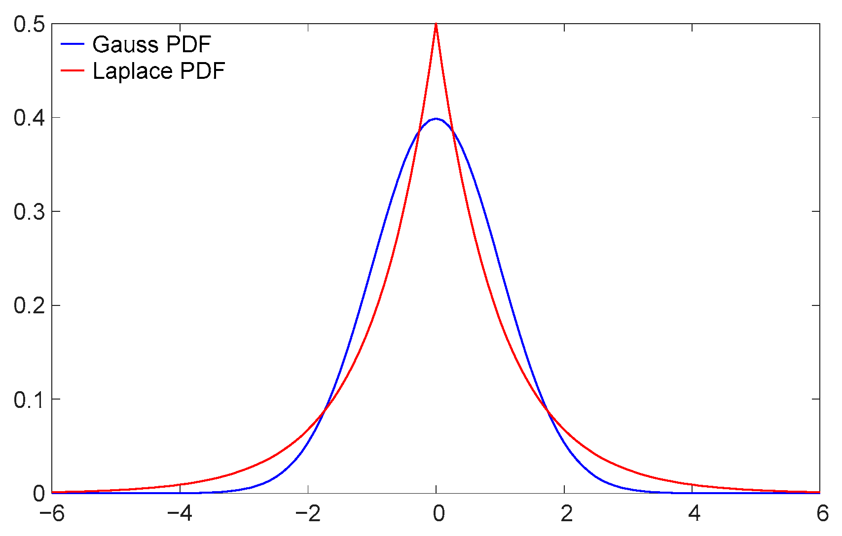
(1) The algorithm employs the Laplace distribution instead of the conventional Gaussian distribution to generate members of state vector ensembles. The general behavior of the Laplace distribution resembles the Gaussian distribution but includes a higher incidence of outliers. This feature allows the algorithm to more closely mimic the real system state in natural environments, thereby improving the algorithm’s robustness to non-Gaussian noise.

(2) The adaptive mechanism allows the algorithm to dynamically adjust the number of members in the state vector ensemble based on an evaluation of the smoothness of the filtered trajectory and the credibility of filtering outputs. This enables the algorithm to adaptively modify its performance according to the actual demand on smoothness and accuracy thus enhancing the efficiency for real-time navigation.

(3) AUV navigation data obtained from field tests is used for the parameter optimization and performance validation of our proposed filtering algorithm. The advantages of the enhanced adaptive EnKF algorithm are demonstrated through comparisons with other filtering algorithms.

The rest of this paper is organized as follows: Section 2 introduces the AUV platform and the hardware configuration of its integrated navigation system in this study. Section 3 presents the model and the parameters involved in our proposed EnKF algorithm, and also describes our sample generation method derived from the Laplace distribution. In Section 4, the key parameters of the algorithm are tuned based on AUV field data to optimize algorithmic performance. Section 5 introduces our adaptive mechanism into the algorithm, enabling it to adjust the number of generated sample ensembles based on the smoothness of the filtered trajectory curves and the credibility of filtering outputs. We explain the comparison between our enhanced EnKF algorithm with standard algorithms such as the conventional EnKF and EKF in Section 6. The last section summarizes the findings in the research and the future directions.

2. AUV Platform and Sensors

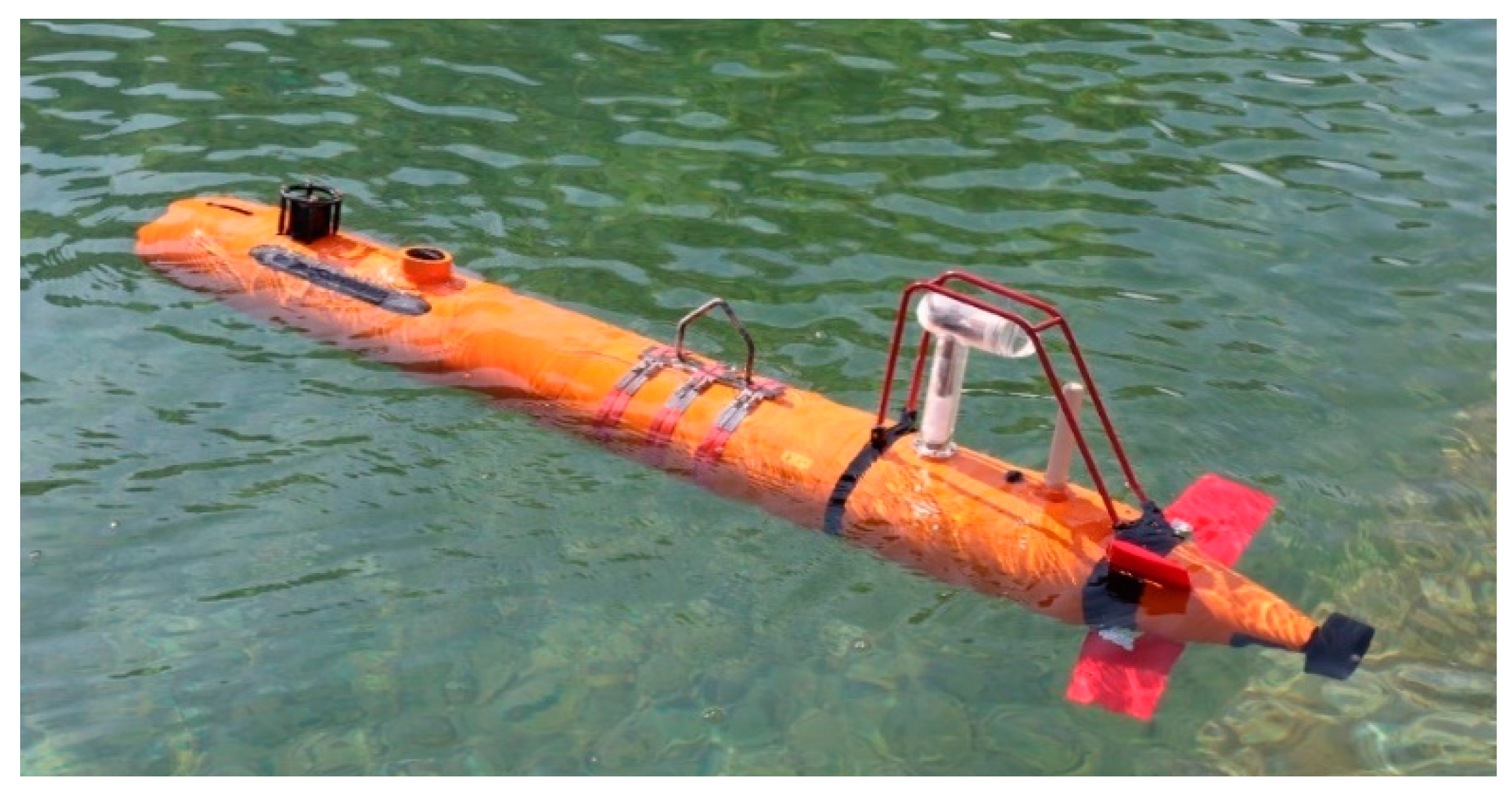
This section introduces the AUV platform as well as its navigation sensors involved in this study. The vehicle is 1.8 m in length and has a diameter of 0.2 m. The maximum working depth is 120 m and the nominal forward running speed is 1 m/s, with the maximum speed of 2 m/s [33]. The vehicle is designed into three modules: an observation module at the bow (capable of 180° rotation for both sea bottom and ice bottom mapping), a navigation and control module in the middle, and a propulsion module at the stern.

The AUV platform used in this study, as shown in Figure 1, is equipped with an array of sensors to perform various observational tasks efficiently. These sensors include the following: a Conductivity, Temperature, Depth sensor for measuring the physical properties of marine water, a DVL for water current measurement, an echosounder for altimeter measurement, a side-scan sonar for topography mapping, and a multi-beam sonar for underwater imaging. These sensors collectively enable comprehensive data collection for marine research and exploration.

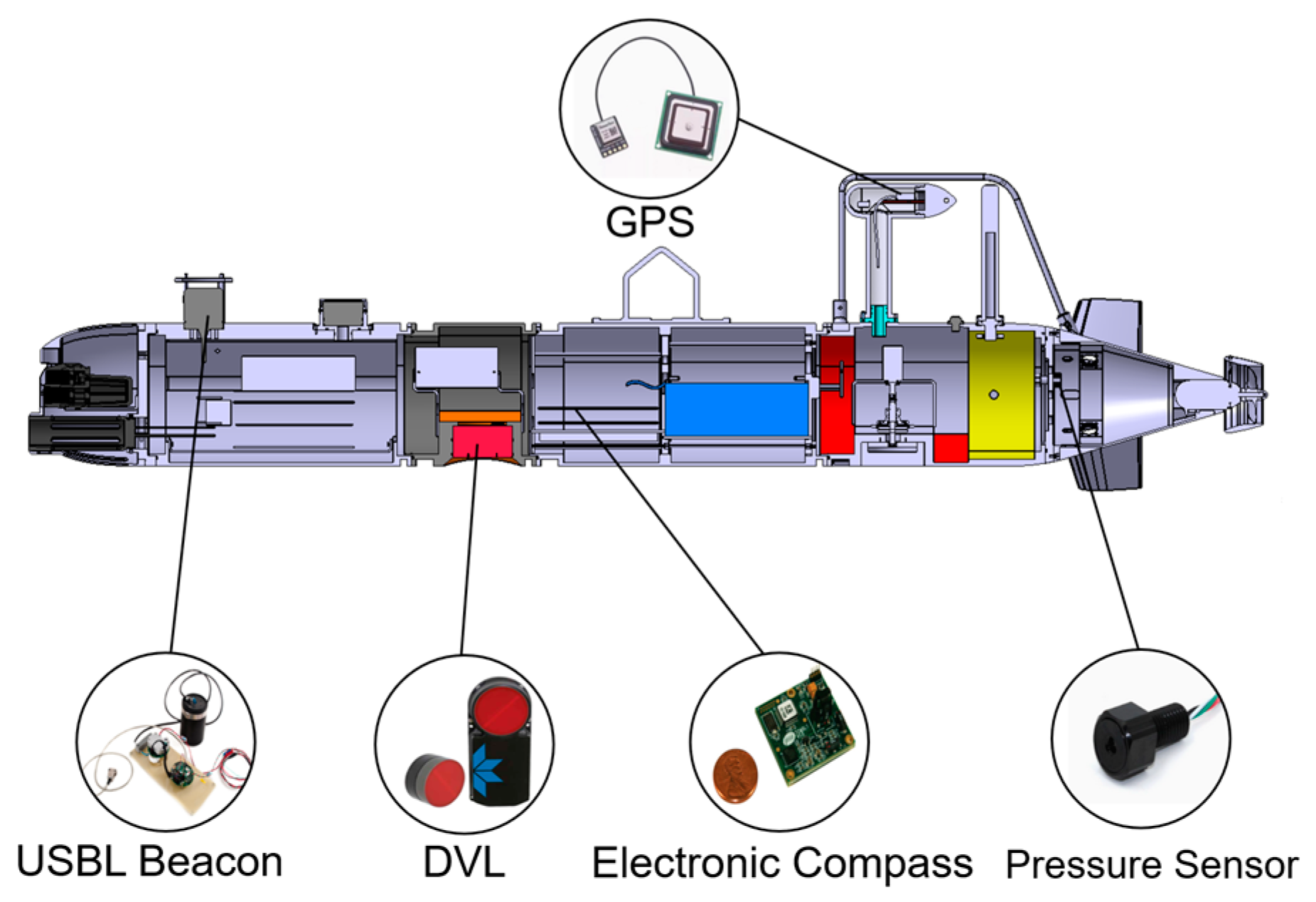
The AUV’s navigation system, as shown in Figure 2, comprises several key components: a USBL, a GPS receiver, a DVL, an electronic compass, and a pressure sensor.

The USBL in Figure 2 is an EvoLogics S2CR 18/34 model with a measurement range of 3500 m, slant range accuracy of 0.01 m, and bearing resolution of 0.1°. It provides acoustic positioning data for the AUV. The Teledyne RD Instruments Pathfinder 600 kHz phased array DVL (Teledyne RD Instruments, Poway, CA, USA) is utilized for both bottom and water mass tracking. Its primary function is to gather data on the AUV’s navigation speed and measure water flow rates with a long-term accuracy of approximately ±0.2% or ±0.1 cm/s. Additionally, the DVL enables the measurement of the AUV’s clearance from the seabed, with a maximum range of up to 150 m. The system also includes a FieldForce TCM electronic compass (PNI Sensor Corporation, Santa Rosa, CA, USA), which delivers precise heading data. This compass boasts a resolution of 0.1 degrees and a tilt accuracy of 0.2 degrees RMS (root mean square). Lastly, the pressure sensor measures pressures up to 20 bar with an accuracy of 0.05% full scale under specified temperature conditions. Together, these components form a robust navigation system, enabling the AUV to perform precise and reliable underwater operations if a proper filtering algorithm is well developed. Furthermore, the core computational platform utilized in the AUV is the LattePanda Alpha 864s dev kit, equipped with 8 GB of LPDDR3 memory and an Intel 8th generation m3-8100y processor, which has a base frequency ranging from 1.1 to 3.4 GHz, supporting dual-core and quad-thread processing.

Figure 3 shows the structure of the hardware system in the AUV of the study. The aforementioned sensors onboard the AUV communicate with the AUV processor via a serial interface, transmitting sampled data to the processor at a certain frequency. Under the control of the central master clock, time synchronization is achieved. This master clock broadcasts time signals to all sensors, ensuring they operate on a unified time basis. During the mission, the master clock is calibrated using GPS signals to establish a high-precision time reference thereby ensuring synchronization. Additionally, during data recording, each sensor adds high-precision timestamps to the recorded data. These timestamps are synchronized with the master clock, enabling precise time alignment for subsequent data fusion and analysis.

The field test navigation data collected from our AUV platform will be saved and exported as a time series dataset in .txt format. This dataset will then be processed using MATLAB R2022b software for data loading, preprocessing, and visualization of the selected results. The processed data will subsequently be utilized on the Python platform for developing and implementing the algorithm proposed in this study.

3. Setup of Our Proposed Ensemble Kalman Filter

This section will present the fundamental components and workflow of our enhanced adaptive EnKF algorithm. This algorithm fuses multi-sensor data to deliver accurate navigation information for vehicle control.

3.1. General Framework of Kalman Filter

3.1.1. Kalman Filter

Kalman filter (KF) is a recursive algorithm designed for optimal state estimation in time-varying linear systems. Its operation is mainly divided into prediction and correction phases, which allows the prediction of system states and the integration and updating of these predictions with observed values thus reducing the variance of prediction errors for future states [34]. Initially, we denote a system state vector $x_k$, which is assumed to contain a set of values describing the state of the system at time $k$. This allows the state from the previous time step to be propagated to time $k$, leading to the state transition equation for the KF as follows:

$$x_k=F{x}_{k-1}+B{u}_{k-1}+{\omega }_{k-1}$$

(1)

where $F$ denotes the state transition matrix, defining the relationship of system state variables as they evolve over time; $u_{k-1}$ represents the external input to the system at the previous time step; $B$ refers to the control matrix, indicating how external inputs influence the state of the system; and ω denotes the process noise, accounting for errors due to external uncertainties that cannot be entirely predicted by the system model. The system model of the algorithm often exhibits inevitable and unpredictable discrepancies compared to the actual system. These discrepancies may arise from internal uncertainties within the system or from external random disturbances. To mitigate these effects, it is essential to incorporate suitable process noise to enhance the model’s robustness against environmental disturbances and to improve the precision of state estimations.

To facilitate the transition from system state variables to observable output quantities, the following observation equation is formulated as follows:

$$z_k=H{x}_k+{\upsilon }_k$$

(2)

where $z_k$ represents the system observation vector; $H$ denotes the observation matrix, delineating how system states influence observed values and facilitating their mapping into the observation space; and $v_k$ describes the system’s measurement noise, which encompasses the random errors resulting from the uncertainties encountered during the measurement process. These uncertainties primarily originate from the inherent precision limitations of sensor equipment and distortions occurring during signal transmission. Furthermore, since the KF is primarily designed for linear Gaussian systems, both the process noise ω and the measurement noise $\upsilon$ are typically assumed to consist of random variables that are independent from each other, follow a Gaussian distribution, and have a zero mean. Therefore,

$$\begin{array}{l}{\omega }_k~N\left(0,Q\right),\\ {\upsilon }_k~N\left(0,R\right)\end{array}$$

(3)

where $Q$ and $R$, respectively, denote the covariance matrices of process noise and measurement noise.

The uncertainty associated with the state prediction from the preceding time step is propagated to the current time step via the state error covariance matrix, as described in Equation (4) as follows:

$$P_{\overline{k}}=F{P}_{k-1}{F}^T+Q$$

(4)

where $P_{k-1}$ is the state error covariance matrix corresponding to time $(k-1)$ and $P_{\overline{k}}$ denotes the prior state error covariance matrix at time $k$.

As previously stated, Equations (1), (2) and (4) collectively constitute the predictive component of the computational expressions in the core iterative algorithm of the KF. Then, the filter integrates the data from the prior state vector estimates and observations based on their respective confidence weights. To facilitate this integration, the KF employs a parameter known as the Kalman gain, which adjusts the relative weights assigned to the estimates and observations. This computation is specified as follows:

$$K_k={\displaystyle \frac{P_{\overline{k}}{H}^T}{H{P}_{\overline{k}}{H}^T+R}}$$

(5)

where $K_k$ represents the Kalman gain at time $k$. Using the Kalman gain value $K_k$ derived from this step, the optimal state estimate vector at time $k$ can be calculated using the following Equation (6):

$$x_k=x_{\overline{k}}+K_k\left(Z_k-H{x}_{\overline{k}}\right)$$

(6)

where $x_k$ refers to the posterior estimate of the state vector at time $k$ following filtering optimization and $x_{\overline{k}}$ denotes the prior predictive state vector value at time $k$ described in Equation (1). After the state vector is corrected through filtering, the error covariance matrix needs to be updated in accordance with the procedure outlined as follows:

$$P_k=\left(I-K_{k}H\right)P_{\overline{k}}$$

(7)

where $I$ is the identity matrix, which has the same dimensions as the state vector $x_k$, and $P_{\overline{k}}$ represents the prior error covariance matrix at time $k$, which has been derived in Equation (4).

Equations (1), (2) and (4)–(7) collectively constitute the core iterative equations utilized within the KF computation at a given time step. The posterior estimates $x_k$ and the error covariance matrices $P_k$ are then conveyed to the subsequent time step to continue the filtering process as described.

3.1.2. From KF to EnKF

The Ensemble Kalman filter (EnKF) is a nonlinear filtering algorithm that combines the KF with the Monte Carlo method. It constructs a sample ensemble to take the place of the covariance matrix operation in the KF, which enhances the filter’s effectiveness in dealing with nonlinear systems, offering significant improvements in handling the inherent complexity of such models. The EnKF involves the use of ensembles of randomly generated state vector samples to approximate and recover the statistical properties of the actual system state thus replacing the traditional error covariance matrix in the iterative computations. It uses a finite set of states to approximate the statistical properties of the system states, implicitly estimating the error covariance matrix through the variance between the sample ensembles. This approach avoids the direct manipulation of large error covariance matrices encountered in the conventional KF algorithm on large systems, and significantly reduces the computational resource consumption when dealing with high-dimensional systems [35]. Starting from the initial state vector $x_k$, random perturbations are applied to generate a corresponding ensemble of state vector samples, which are structured as follows:

$$X_k=\left[x_1^k,x_2^k,x_3^k,\cdots ,x_n^k\right]$$

(8)

where $X_k$ corresponds to the ensemble of random samples representing the system state vector at time $k$ and $n$ indicates the number of members in this ensemble. Similarly, based on the initial observation vector $z_k$, the observation vector sample ensemble $Z_k$ is defined as follows:

$$Z_k=\left[z_1^k,z_2^k,z_3^k,\cdots ,z_n^k\right]$$

(9)

As a substitute for estimating and updating the error covariance matrix, compute the mean of the generated state vector sample ensemble ${\overline{X}}_k$ as follows:

$${\overline{X}}_k={\displaystyle \frac{\sum _{i=1}^n{x}_i^k}{n}}$$

(10)

Furthermore, we can utilize the ensemble mean to execute the calculation outlined below, which serves to replace the iterative and corrective steps involving the error covariance matrix, as traditionally performed in the KF Equations (4) and (7).

$$P_H={\displaystyle \frac{\sum _{i=1}^n(x_i^k-{\overline{X}}_k\left)\right(H{x}_i^k-H{\overline{X}}_k)}{n-1}}$$

(11)

where $P_H$ represents an intermediate variable that substitutes for the traditional error covariance matrix thereby facilitating the implicit propagation of error covariance. Once $P_H$ has been computed, it is incorporated into Equation (5) to directly calculate the Kalman gain.

$$K_k={\displaystyle \frac{P_H}{H{P}_H+R}}$$

(12)

Additionally, modifications based on Equation (6) yield the filtering optimization correction formula for the state vector under the EnKF algorithm as follows:

$$x_k={\displaystyle \frac{\sum _{i=1}^n{[x}_i^k+K_k\left(z_i^k-H{x}_i^k\right)]}{n}}$$

(13)

From Equation (13), one can derive the EnKF algorithm’s filtering estimation for the current time step. The operations detailed in Equations (8)–(13) outline the principal computational steps of the EnKF algorithm. As the algorithm progresses to the subsequent time step, the process is initiated anew from Equation (8) with the reconstruction of the state vector’s random sample ensemble, followed by the subsequent calculations.

3.2. AUV State Model and Settings

In this study, the EnKF algorithm is utilized to address AUV qualitative navigation issues within a given area. To simplify the problem, we consider AUV navigation in the horizontal plane, so that AUV speed measured by DVL, attitude measurements from the electronic compass, and position data from the GPS are taken into account in the filtering algorithm. In this section, we will focus on the development of AUV system equations and variables that are specifically tailored to the EnKF algorithm.

Generally, AUV’s position $X={[x,y,z]}^T$ is described in the inertial coordinate frame, represented by an orthonormal triad $\{x,y,z\}$, where $z$ is aligned with the local direction of gravity. However, AUV’s velocity $v={[u,v,w]}^T$ is measured in the body-fixed coordinate frame, defined by an orthonormal triad $\{x_b,y_b,z_b\}$, where $\{x_b,y_b,z_b\}$ is aligned with the body’s longitudinal axis [36]. The origin of the body frame sits at the vehicle’s center of buoyancy. A proper rotation matrix $\mathcal{R}$, parameterized by the Euler angles, is used to map free vectors from the body-fixed frame to the inertial frame. The Euler angles include the roll angle $\varphi$, the pitch angle $\theta$, and the yaw angle $\psi$, which are depicted in Figure 4.

The rotation matrix $\mathcal{R}$ is defined as follows [37]:

$$\begin{gathered} \mathcal{R}=\left[\begin{array}{cc}\mathit{cos}\left(\psi \right)\cos \left(\theta \right)& -\mathit{sin}\left(\psi \right)\mathit{cos}\left(\varphi \right)+\mathit{cos}\left(\psi \right)\mathit{sin}\left(\theta \right)\sin \left(\varphi \right)\\ \mathit{sin}\left(\psi \right)\cos \left(\theta \right)& \mathit{cos}\left(\psi \right)\mathit{cos}\left(\varphi \right)+\mathit{sin}\left(\psi \right)\mathit{sin}\left(\theta \right)\sin \left(\varphi \right)\\ -\sin \left(\theta \right)& \mathit{cos}\left(\theta \right)\sin \left(\varphi \right)\end{array}\right. \cdots \\ \left.\begin{array}{c}\mathit{sin}\left(\psi \right)\mathit{sin}\left(\varphi \right)+\mathit{cos}\left(\psi \right)\mathit{sin}\left(\theta \right)cos\left(\varphi \right)\\ -\mathit{cos}\left(\psi \right)\mathit{sin}\left(\varphi \right)+\mathit{sin}\left(\psi \right)\mathit{sin}\left(\theta \right)cos\left(\varphi \right)\\ \mathit{cos}\left(\theta \right)cos\left(\varphi \right)\end{array}\right] \end{gathered}$$

(14)

Consequently, by multiplying the rotation matrix $\mathcal{R}$ with the velocity vector $v$, one obtains the AUV’s velocity vector expressed in the inertial frame.

$$V={[v_x,v_y,v_z]}^T=\mathcal{R}\cdot v$$

(15)

This process allows the establishment of the state vector of AUV dynamic system in the inertial frame, which includes AUV kinematic parameters.

$$x_{state}={\left[x,y,z,v_x,v_y,v_z\right]}^T$$

(16)

Assuming that the sensors sample the AUV’s motion data at intervals of $dt$, one can derive the kinematic equation shown in Equation (17). This equation employs the AUV’s motion states at the previous moment in conjunction with the data sampled from the sensors to calculate the motion states at the current moment.

$$x_{state,k}=\left[\begin{array}{c}{x}_k\\ y_k\\ z_k\\ v_{x,k}\\ v_{y,k}\\ v_{z,k}\end{array}\right]=\left[\begin{array}{c}{x}_{k-1}+v_{x,k}dt\\ y_{k-1}+v_{y,k}dt\\ z_{k-1}+v_{z,k}dt\\ v_{x,k}\\ v_{y,k}\\ v_{z,k}\end{array}\right]=\left[\begin{array}{cccccc}1& 0& 0& dt& 0& 0\\ 0& 1& 0& 0& dt& 0\\ 0& 0& 1& 0& 0& dt\\ 0& 0& 0& 1& 0& 0\\ 0& 0& 0& 0& 1& 0\\ 0& 0& 0& 0& 0& 1\end{array}\right]\left[\begin{array}{c}{x}_{k-1}\\ y_{k-1}\\ z_{k-1}\\ v_{x,k}\\ v_{y,k}\\ v_{z,k}\end{array}\right]=F{x}_{k-1}$$

(17)

where $F$ indicates the state transition matrix of the system. Then, the AUV’s positional and velocity data are utilized to compile the observation vector z. Since the AUV’s positioning information $X=[x,y,z]$ comes from the observed data, following Equation (2), the observation matrix $H$ is defined as follows:

$$H=\left[\begin{array}{cccccc}1& 0& 0& 0& 0& 0\\ 0& 1& 0& 0& 0& 0\\ 0& 0& 1& 0& 0& 0\end{array}\right]$$

(18)

Thus far, we have derived describe the AUV motion system by Equations (14)–(18).

3.3. Generation of State Vector Ensemble

EnKF necessitates the creation of a sample ensemble by adding random perturbations to the state vector to simulate model errors. The real error covariance is approximated through the distribution of members in the ensemble [38]. Therefore, generating a random ensemble with an appropriate distribution rule is crucial for the filtering performance of the EnKF algorithm. In this subsection, the Laplace distribution function is introduced into EnKF, and its effectiveness is compared with the conventional Gaussian distribution function to demonstrate its advantages.

The Gaussian distribution is characterized by its broad and general statistical properties. Filtering algorithms such as the EKF and EnKF typically assume that both system and observation errors adhere to a Gaussian distribution during the linear approximation of nonlinear systems. The probability density function for the Gaussian distribution is as follows:

$$f\left(x|\mu ,{\sigma }^2\right)={\displaystyle \frac{1}{\sqrt{2\pi {\sigma }^2}}}\mathrm{e}\mathrm{x}\mathrm{p}\left[-{\displaystyle \frac{{\left(x-\mu \right)}^2}{2{\sigma }^2}}\right]$$

(19)

where $x$ denotes a random variable; $\mu$ represents the mean value of the distribution; and $\sigma$ refers to the standard deviation of the distribution.

EnKF generates ensembles by adding zero-mean Gaussian-distributed perturbations to the state vector, simulating uncertainties inherent in real systems [39]. However, in actual AUV navigation tasks, dynamic ocean processes, human activities, and sensor errors may introduce significant non-Gaussian noise disturbances, which are characterized by large impulses, short durations, and pronounced tails. This makes Gaussian-based sample generation inadequate for accurate state approximation. To improve robustness against non-Gaussian noise, alternative sample generation methods are essential.

The Laplace distribution, also known as the double exponential distribution, derives its name from its graphical resemblance to the combined representation of two exponential distribution probability density functions. It is defined by a location parameter and a scale parameter, with its probability density function given by Equation (20).

$$f\left(x|\mu ,b\right)={\displaystyle \frac{1}{2b}}exp\left(-{\displaystyle \frac{\left|x-\mu \right|}{b}}\right)$$

(20)

where $\mu$ denotes the location parameter, indicating the mean value of the distribution, and $b$ represents the scale parameter, which determines the distribution’s spread; this value is estimated by $b={\displaystyle \frac{1}{n}}\sum |x^i-\mu |$ in this study. The introduction of additional parameters on this basis enables the development of various Laplace distribution variants, making it versatile enough to accommodate different research questions and data characteristics [40].

Figure 5 presents a comparative graph of the function curves for the standard Gaussian distribution ($\mu =0, \sigma =1$) and the standard Laplace distribution ($\mu =0, b=1$). Both distributions exhibit a comparable functional form and overall distribution trend. However, the Laplace distribution’s curve, as illustrated in Figure 5, features a more pronounced peak and thicker tails compared to the Gaussian distribution. This indicates that, while maintaining properties similar to the Gaussian distribution, the Laplace distribution is more prone to include extreme values or outliers, providing a more accurate reflection of the statistical characteristics for systems with significant non-Gaussian noise.

The Laplace distribution is extensively utilized in various fields, including finance and industry. It is often employed as an alternative to the Gaussian distribution in robustness research [40]. This distribution is characterized by the maximum entropy property, meaning it exhibits the highest level of entropy among all probability distributions with a given mean and variance. This results in greater uncertainty and informational content under comparable conditions, making the Laplace distribution particularly valuable for both practical applications and scholarly research [41].

To further verify the effectiveness of the Laplace distribution in modeling the positioning deviations of AUV in underwater conditions, the deviation between the actual navigation trajectory and the predefined trajectory at each sampling point during the AUV field test was calculated. Figure 6 depicts the probability density distribution curve of the aforementioned deviation, along with the Gaussian and Laplace distribution curves, which exhibit the same mean and standard deviation as the deviation data. As illustrated in the figure, the probability distribution of the AUV positioning trajectory exhibits pronounced peaks and relatively thick tails, closely approximating the probability density curve of the Laplace distribution.

Moreover, we employ the Akaike Information Criterion (AIC) to quantify and compare the fit of the trajectory error distribution with two specific distribution functions. AIC derives from the concept of entropy, which is a widely utilized metric for assessing the goodness of fit between models or distributions and observed data [42]. For the same dataset, a lower AIC value indicates a superior fit of the distribution to the data.

The definition of AIC is given by Equation (21) as follows:

$$AIC=2k-2\ln \left(L\right)$$

(21)

where $k$ represents the number of parameters in the formula of the distribution function, and $k$ is equal to 2 for both the Gaussian and Laplace distributions; $L$ denotes the log-likelihood function corresponding to the probability density function of the two distributions, as shown for the Gaussian distribution in Equation (22) and for the Laplace distribution in Equation (23).

$$\begin{gathered} \ln \left(L_{gauss}\right)=\sum _{i=1}^n\ln \left[{\displaystyle \frac{1}{\sqrt{2\pi {\sigma }^2}}}\exp \left(-{\displaystyle \frac{{\left(x_i-\mu \right)}^2}{2{\sigma }^2}}\right)\right] \\ =-{\displaystyle \frac{n}{2}}\ln \left(2\pi {\sigma }^2\right)-{\displaystyle \frac{1}{2{\sigma }^2}}\sum _{i=1}^n{\left(x_i-\mu \right)}^2 \end{gathered}$$

(22)

$$\begin{gathered} \ln \left(L_{laplace}\right)=\sum _{i=1}^n\ln \left[{\displaystyle \frac{1}{2b}}\exp \left(-{\displaystyle \frac{|x_i-\mu |}{b}}\right)\right] \\ =-n\ln \left(2b\right)-{\displaystyle \frac{1}{b}}\sum _{i=1}^n|x_i-\mu | \end{gathered}$$

(23)

Using Equations (21)–(23), the AIC value for the Gaussian distribution applied to the positioning deviation data is calculated as 366,986.314, while the value for the Laplace distribution is 295,339.704. These values indicate that, according to the AIC, the Laplace distribution provides a superior representation of the deviation distribution in the AUV’s navigation trajectory. It should be noted that the sample size of the dataset significantly impacts the numerical value and magnitude of the AIC. Therefore, the absolute value of the AIC has no specific meaning, only the relative size of the AIC values between the two distributions should be considered. The AUV trajectory deviation dataset in Figure 6 contains 60,000 samples, which results in a correspondingly high magnitude for the AIC values of both distributions.

Consequently, employing datasets that adhere to the Laplace distribution enhances the EnKF algorithm’s ability to adapt to non-Gaussian noise. This adaptation allows for more accurate approximations of systems within actual marine environments and increases the stability of the algorithm’s positioning capabilities. Therefore, in the EnKF algorithm we proposed, the random perturbations representing process noise and measurement noise added during the generation of the vector ensemble follow a Laplace distribution thus transforming Equation (3) to the following:

$$\begin{array}{l}{\omega }_k~Laplace\left(0,Q_{Lap}\right),\\ {\upsilon }_k~Laplace\left(0,R_{Lap}\right)\end{array}$$

(24)

where $Q_{Lap}$ and $R_{Lap}$ represent the covariance matrices of process noise and measurement noise, respectively, both following Laplace distribution.

3.4. Summary of EnKF Operational Procedures

In this subsection, we have summarized the overall framework of the EnKF and the method for generating vector samples within the algorithm. Figure 7 illustrates the operational flowchart of the EnKF, which estimates and updates the system state through multi-sensor data fusion and state optimization prediction. As shown in Figure 7, velocity information {$u,v,w\}$ from DVL and attitude information $\{\theta ,\phi ,w\}$ from the electronic compass is fused to provide dead reckoning data $\{v_x,v_y,v_z$}. These measurements combined with the system state from the previous iteration yield the current system state vector $x_k$. Meanwhile, GPS data builds the observation vector $z_k$, which, along with $x_k$, generates the corresponding observation and state vector ensembles $Z_k$ and $X_k$, respectively, by adding random disturbances ${\omega }_{ps}$ and ${\omega }_{po}$ that represent process noise. The system then calculates $X_k$ using the observation matrix $H$, resulting in the intermediate variable $P_H$, which implicitly reflects the state error covariance of the system. Further, the matrix $R$, which represents measurement noise, is introduced to compute the Kalman gain $K_k$. Using the Kalman gain, $X_k$ and $Z_k$ are integrated with specific weights to produce the final filtered state vector $x_k^{*}$. Among these factors, the parameters ${{\sigma }_{po}}^2$ and ${{\sigma }_{ps}}^2$, which affect the magnitude of process noise, as well as the parameters ${{\sigma }_{obs}}^2$ and ${{\sigma }_v}^2$, which influence the measurement noise $R$, play a significant role in the filtering performance of the algorithm. In the next section, we will discuss and analyze the values of these parameters to identify a relatively optimal parameter configuration.

4. Optimization of Parameters in EnKF

This section will focus on tuning the parameters of the EnKF algorithm based on data from field trials. The tuning process will utilize the method of controlled variables, systematically adjusting and analyzing the impact of different parameter changes on the filtering performance of the algorithm. This approach will guide the optimization of parameters, ultimately aiming to enhance the precision of the filtering process.

4.1. Data Sources

The AUV navigation data used in this study were collected from field trials conducted in the coastal waters surrounding Jiangmen City, Guangdong Province, China, between 31 May and 2 June 2022. The test area was located at 21°50′ N, 112°55′ E, as illustrated in Figure 8. During the field tests, the AUV navigates at the water’s surface, enabling it to obtain positioning information via GPS, although this information exhibited some instability and positioning fluctuations. This instability arises from the sensitivity of GPS signals to various environmental interference factors. When the AUV navigates on the surface in the dynamic ocean environment, the effects of wind and waves cause repeated changes in the air–sea interface, with factors such as bubbles and waves potentially interfering with GPS signal reception. Near the surface, GPS signals entering the receiving antenna through different reflected paths are subject to multipath effects, leading to possible signal delays, attenuation, or brief losses, which can result in short-term fluctuations in positioning data. These fluctuations may introduce significant instantaneous errors into positioning information. If such interference persists, the influence of instantaneous errors can accumulate when GPS signals are used to correct INS positioning data, potentially causing significant long-term drift, which compromises positioning accuracy. Furthermore, if the AUV’s receiving antenna is submerged in water, it may lead to a decrease in the frequency of received positioning signals or even temporary loss of signals. Although the AUV navigation data used in this study did not experience complete GPS signal loss, it remains an important factor to consider for ensuring GPS positioning accuracy during real missions. Therefore, mitigating the impact of these factors through the integration and processing of navigation data is one of the primary objectives of our proposed algorithm.

The example trajectories of the AUV’s dead reckoning and the GPS positioning, derived from the test data, are depicted in Figure 9. This figure includes the data spanning approximately 4000 time steps, with each step sampled at intervals of about 0.2 s. It is evident that the discrepancy between the dead reckoning and GPS positioning trajectories shown in Figure 9 increases over time, leading to a significant deviation at the end of the motion.

In this section, we aim to refine the EnKF algorithm to process sensor data, including speed, attitude, and GPS fix data collected from the AUV field trials. By integrating dead reckoning data with GPS information, the study seeks to mitigate the cumulative positioning errors inherent in dead reckoning over time and correct for the GPS positional drift and fluctuations caused by environmental disturbances during experiments [43]. In order to visually illustrate the optimization effect of the algorithm on the GPS information subsequent to the integration of dead reckoning data, GPS positioning data will be employed as a baseline for the comparison and evaluation of the filtering performance of the algorithm under different parameter settings in this section.

4.2. Impact of Key Parameters on EnKF Filtering Performance

In the algorithm utilized in this study, the measurement noise and process noise, represented by the ensemble covariance, cannot be adjusted iteratively by the filter and must be pre-set as key parameters. They describe the accuracy and reliability of system state estimates and directly influence the manner in which the filter strikes a balance between trusting system predictions and measurement data. This balance has a significant impact on the accuracy and stability of the state estimation. Therefore, this subsection will explore how different values of measurement noise and process noise affect the algorithm’s filtering performance through a series of tests, providing guidance for optimizing filter performance.

4.2.1. Process Noise

Process noise is a measure of the inherent uncertainty of a system model in relation to actual conditions. Intrinsically, in the EnKF algorithm, the model’s uncertainty will be captured and approximated by adding perturbations to each member of a vector ensemble according to a specified distribution and analyzing the statistical characteristics of the ensemble. Consequently, explicit propagation of process noise through Equation (5) is unnecessary in the EnKF. Thus, adjusting the process noise parameters in the EnKF fundamentally involves tuning the variance of the random perturbations introduced into the generated state vector ensemble.

To investigate the impact of variance changes in the sample vector ensembles on the filtering effectiveness of the EnKF algorithm and to provide guidance for algorithm parameter tuning, we generate sample ensembles with a quantity of 100, a variance of 1, and no measurement noise. All the other parameter adjustment conditions will be made in relation to this baseline.

(1) Variance of the observation vector ensemble ${{\sigma }_{po}}^2$

In the scenario where no measurement noise is present and a state vector ensemble of size 100 is generated using a Laplace distribution with a scale parameter of 1, we examine the influence of varying variances in the observation vector ensembles on the EnKF’s filtering performance.

Figure 10 shows a partial enlarged view of EnKF’s filtering trajectories and GPS positioning curves during AUV turning motion under different ${{\sigma }_{po}}^2$ values. When ${{\sigma }_{po}}^2=0.1$, the green curve in Figure 10a, the EnKF filtered trajectory nearly aligns with the GPS results, maintaining smoothness. At ${{\sigma }_{po}}^2=1$, the blue curve in Figure 10b, the trajectory still aligns closely with GPS, but noticeable fluctuations appear between 330 m and 340 m on the $x$-axis, reducing smoothness. At ${{\sigma }_{po}}^2=1$0, the red curve in Figure 10c, the filtered result fails to converge stably, showing significant fluctuations.

The results of the parameter adjustment shown in Figure 10 indicate that an increase in the variance of the observation vector ensemble correlates with a high degree of filtered trajectory fluctuation. Specifically, in the baseline parameter setting condition, setting the variance parameter to 10 leads to a significant instability in system filtering. This highlights the necessity of calibrating the variance parameters in the observation vector ensemble relative to the scale of the actual observational data. Such calibration ensures that the ensemble can accurately reflect the potential error distribution of the system without compromising stability due to overly high variance values.

(2) Variance of the state vector ensemble ${{\sigma }_{ps}}^2$

The adjustment test for the variance of the state vector set is analogous to that of the observation vector ensemble described above. The results of the test indicate that, with the current parameter settings, modifying the variance of the state vector ensemble does not significantly affect the filtering performance of the EnKF. Even when the value of ${{\sigma }_{ps}}^2$ is increased from 0.01 to 100, the algorithm’s filtering performance remains largely unchanged, with the filtered trajectory closely aligned with the GPS positioning trajectory. This outcome underscores that, in the current setup, the algorithm disproportionately relies on GPS positioning data, largely overlooking the positional estimates derived from dead reckoning. Therefore, future adjustments are needed to account for different settings of measurement noise in order to refine the algorithm’s performance.

4.2.2. Measurement Noise

Measurement noise represents the inherent uncertainty in the gathering of sensor data and significantly impacts filter performance, which is similar to the process noise [44]. To better approximate measurement errors, Kalman filter measurement noise should be tailored to sensor capabilities. In the absence of precise references, optimal measurement noise can be determined experimentally. In this study, the AUV’s position and orientation in three-dimensional space are derived from sensor observations, assuming independent measurement noise in the $x$, $y$, and $z$ axes with equal variance. This assumption leads to the fundamental form of the measurement noise covariance matrix in Equation (25).

$$R=\left[\begin{array}{ccc}{\sigma }_{obs}^2& 0& 0\\ 0& {\sigma }_{obs}^2& 0\\ 0& 0& {\sigma }_{obs}^2\end{array}\right]$$

(25)

where ${\sigma }_{obs}^2$ denotes the variance of the sensor measurement noise and serves as the scalar factor in the covariance matrix. Subsequently, the model incorporates additional random perturbations ${\upsilon }_{ij} (i,j=1, 2, 3)$ with a mean of zero, derived from a Laplace distribution, which are superimposed upon the foundational measurement noise covariance matrix. In this matrix, the variance of ${\upsilon }_{ij}$ is denoted by ${\sigma }_v^2$. This setup leads to the result as shown in Equation (26).

$$R=\left[\begin{array}{ccc}{\sigma }_{obs}^2+{\upsilon }_{11}& {\upsilon }_{12}& {\upsilon }_{13}\\ {\upsilon }_{21}& {\sigma }_{obs}^2+{\upsilon }_{22}& {\upsilon }_{23}\\ {\upsilon }_{31}& {\upsilon }_{32}& {\sigma }_{obs}^2+{\upsilon }_{33}\end{array}\right]$$

(26)

Subsequently, experiments will be conducted to separately investigate how variations in ${\sigma }_{obs}^2$ and ${\sigma }_v^2$ within the matrix affect the algorithm’s filtering performance, with the objective of confirming the value selection for the matrix $R$ in the algorithm.

(1) Variance of the sensor measurement noise ${\sigma }_{obs}^2$, diagonal elements in $R$

To investigate the impact of diagonal elements in matrix $R$ on the filtering algorithm, the ensemble variance is set to 1 for all 100 members, with ${\upsilon }_{ij}$ values at zero and ${\sigma }_{obs}^2$ values at 0.1, 1, and 10, respectively. The partial enlarged view of the EnKF filtering trajectory curves and the GPS positioning curves with different ${\sigma }_{obs}^2$ values is presented in Figure 11. This figure provides a detailed illustration of the impact of the ${\sigma }_{obs}^2$ value on the EnKF filtering results compared with the GPS positioning trajectory. The red curve in Figure 11c, which represents the filtering result with ${\sigma }_{obs}^2=10$, exhibits a notable divergence from GPS data, particularly within the range of 790 $\mathrm{m}$ and 800 $\mathrm{m}$ on the $y$-axis, which smooths the positioning result when AUV is turning. In contrast, no similar deviation is observed with smaller ${\sigma }_{obs}^2$ values. The dead reckoning positioning trajectory exhibits a high level of smoothness. Under the parameter settings represented by the red curve in Figure 11c, the influence of dead reckoning data on the algorithm slightly intensifies, causing a noticeable divergence between the filtered result and GPS positioning data. This divergence manifests as a decrease in the trajectory’s curvature along the general motion direction, making it trend toward a straight line. As a result, this tendency limits the algorithm’s capacity to respond swiftly to abrupt turns made by the AUV. Following a turn, the increased deviation in motion direction and the position hinders the algorithm from quickly recalibrating, leading to a series of short-term fluctuations in the positioning trajectory.

In the context of present conditions, an increase in the measurement noise variance ${\sigma }_{obs}^2$ results in a discernible rise in the fluctuation of the filtering curve, particularly in segments involving significant changes in direction, where deviations from the GPS trajectory become more pronounced. This observation underscores how, with elevated measurement noise, the influence of dead reckoning data on the filtering outcome is amplified, although at the expense of reduced smoothness in parts of the filtering curve. The optimal setting of ${\sigma }_{obs}^2$ is of paramount importance, as values that are either too high or too low will have a detrimental effect on the filter’s performance.

(2) Variance of the model incorporates additional random perturbations ${\sigma }_v^2$

Assume an ensemble variance of 1 and an ensemble members number of 100, with ${\sigma }_{obs}^2$ set at 1, and varying ${\sigma }_v^2$ for ${\upsilon }_{ij}$ at 0.01, 0.1, 0.3, 0.5; the resulting trajectory plots are depicted in Figure 12. As illustrated in the figure, when the value of ${\sigma }_v^2$ is less than 0.5, the filtering results exhibit a high degree of alignment with the GPS positioning data. When ${\sigma }_v^2$ increases to 0.5, as illustrated by the red curve, the filtering trajectory starts to exhibit significant irregular deviations.

In short, based on the experiment results, we conclude that as long as the variance of the random perturbations ${\upsilon }_{ij}$ remains within a predefined acceptable range, its impact on the algorithm’s filtering performance is negligible. However, if the variance is excessively high, it can severely compromise the stability of the filtering results, leading to the generation of anomalies characterized by substantial errors at specific instances.

4.3. Optimization and Comparative Analysis of Parameter Schemes

From the parameter adjustment tests discussed above, we gain the basic understanding of how individual parameters influence the EnKF filtering performance. However, this approach predominantly focuses on single-parameter adjustments thus overlooking the potential synergistic or antagonistic effects that could arise from the interactions between multiple parameters. Consequently, it is necessary to formulate and test combinations of the above discussed parameters that are theoretically optimal, with the aim of refining our strategy based on the insights already acquired.

Based on the discussion in the previous subsection, the preferred parameter configuration is established: assigning a variance of 10 to the observation vector ensemble that represents the process noise and setting the measurement noise within a covariance matrix characterized by a mean influence of 1 and a variance of 0.15.

Figure 13 illustrates a comparison of trajectory curves with different state vector variance settings under the preferred parameter configuration mentioned earlier. As shown in Figure 13a, varying parameter configurations lead to different outcomes in terms of filtering smoothness and divergence from the GPS positioning data, particularly noticeable in the area highlighted by the black box. The enlarged view in Figure 13b shows that as ${{\sigma }_{ps}}^2$ decreases from 0.5 to 0.01, the filtered positioning shifts from close alignment with the GPS trajectory to a deviation toward dead reckoning. Additionally, as ${{\sigma }_{ps}}^2$ decreases, the filtering curve demonstrates an incremental enhancement in its degree of smoothness. In summary, as the variance of the state vector ensemble increases, the filtered trajectory curve becomes increasingly aligned with the GPS trajectory, resulting in a compromise of both smoothness and filtering effectiveness. When ${{\sigma }_{ps}}^2$ reaches a certain threshold, the filtered trajectory tends to completely overlap with the GPS trajectory, and the degree of curve fluctuations increases correspondingly. Conversely, lower values of ${{\sigma }_{ps}}^2$ result in filtering outcomes that more closely resemble dead reckoning estimates, exhibiting a relative increase in smoothness. Consequently, within the parameters considered in this study, adjusting ${{\sigma }_{ps}}^2$ between 0.01 and 0.1 allows for relatively optimal balance between GPS positioning data and dead reckoning estimates while maintaining overall trajectory smoothness.

Based on these findings, this research employs the EnKF algorithm with a state vector ensemble variance of 0.03 for continued investigation.

5. Adaptive Mechanism in EnKF

The previous section investigates the impacts of various algorithm parameters on its filtering performance and achieves parameter optimization by selecting the optimal configurations. In addition to the parameters discussed in Section 4, the number of random samples included in the state vector ensemble generated by the algorithm also influences filtering stability and operational efficacy. The size of this ensemble dictates the sampling density within the system’s state space. Increasing the number of vector samples with random perturbations enhances the model’s ability to approximate the system’s uncertainties and nonlinear features. However, this also increases computational and storage demands thereby increasing the runtime. Conversely, a smaller ensemble of state vector samples may not adequately represent the system’s complexity and uncertainty, potentially compromising the algorithm’s filtering stability. Building on the preceding discussion, this subsection introduces an adaptive mechanism to the EnKF algorithm.

5.1. Key Criteria of Adaptive Mechanism

Our proposed mechanism enables the algorithm to assess the smoothness of the filtered results and the credibility of filtering outputs based on defined criteria, then autonomously adjust the number of ensemble members in the filtering process. This allows for a dynamic equilibrium between filtering stability and real-time performance, tailored to the needs of the navigation system.

5.1.1. Smoothness of Filtering Results

The smoothness of the filtering results reflects the extent of noise reduction and the accuracy of trajectory estimation. Smoother filtering outcomes indicate that the algorithm effectively mitigates noise and accurately captures the true motion pattern of the AUV, resulting in more reliable and stable trajectory predictions.

To evaluate the smoothness of the filtering results, we define a smoothness angle, which is the angle between two lines connecting adjacent trajectory points of the AUV after the filtering process. By computing the average angle of all trajectory points within a specified time interval, we can assess the smoothness of the filtered trajectory. The angle between every three consecutive trajectory points can be determined using the dot product of the corresponding vectors as follows:

$$\overrightarrow{AB}·\overrightarrow{BC}=\left|\overrightarrow{AB}\right|\left|\overrightarrow{BC}\right|\mathit{cos}\left(\theta \right)$$

(27)

where $A,B,C$ represent three consecutive trajectory points, $\overrightarrow{AB}$ and $\overrightarrow{BC}$ are the vectors defined by these points, and $\theta$ is the angle between the two vectors. Assume that the AUV trajectory points estimated by the EnKF algorithm at time $k$ are $(x_k,y_k)$, and the trajectory points at times $(k-1)$ and $(k-2)$ are $(x_{k-1},y_{k-1})$ and $(x_{k-2},y_{k-2})$, respectively. Consequently, the following expression can be derived from Equation (27) as follows:

$${\theta }_{k-1}=\mathrm{a}\mathrm{r}\mathrm{c}\mathrm{c}\mathrm{o}\mathrm{s}{\displaystyle \frac{\left(x_{k-2}-x_{k-1}\right)\left(x_k-x_{k-1}\right)+(y_k-y_{k-1})(y_{k-2}-y_{k-1})}{\sqrt{\left[{(x_{k-2}-x_{k-1})}^2+{(y_{k-2}-y_{k-1})}^2\right]\left[{(x_k-x_{k-1})}^2+{(y_k-y_{k-1})}^2\right]}}}$$

(28)

where ${\theta }_{k-1}$ denotes the angle with respect to the trajectory point at time step $(k-1)$ after filtering.

With Equation (28), we can record the smoothness angle at each trajectory point prior to time $k$. This angle serves as an indicator of the local smoothness of the filtering trajectory at that point. The angle ranges from 0° to 180°, with values closer to 180° indicating better smoothness of the trajectory. By calculating the average smoothness angle of all trajectory points within a specified time interval, we can evaluate the smoothness of the filtering results.

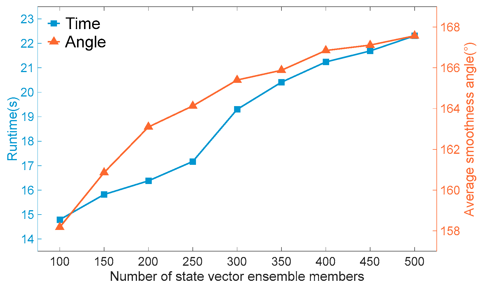
In our study, we find that the number of state vector ensemble members significantly impacts the smoothness of the filtering results. Generally, a larger number of ensemble members leads to a smoother filtered trajectory, but this also increases the filtering runtime, potentially compromising the real-time performance of the filter for online operation. With the given dataset, the variation in runtime and the average smoothness angle of the filter over a specified time period with the number of state vector ensemble members is depicted in Figure 14. The dataset comprises 30,000 sampling points, each separated by approximately 0.2 s, resulting in a total duration of approximately 600 s. As illustrated in Figure 14, an increase in the number of state vector ensemble members results in a smoother filtered trajectory. However, this also leads to a significant increase in the runtime of the filtering algorithm. When the number of ensemble members increases from 100 to 500, the average smoothness angle improves by approximately 10°, while the total runtime rises from approximately 15 s to 22 s, an increase of about 47%.

Based on the method for assessing the smoothness of filtering results mentioned above, an adaptive adjustment mechanism is integrated into the algorithm to dynamically alter the number of state vector members in the ensemble based on predefined thresholds. During the filtering process, a sliding window is used to average a specified number of smoothness angles along the filtered trajectory. This average serves as the quantitative measure of the trajectory’s smoothness. If it exceeds an upper threshold, indicating a sufficiently smooth trajectory, the algorithm will decrease the size of the generated state vector ensemble thereby expediting the processing speed. Conversely, if the average smoothness angle falls below a lower threshold, suggesting substantial fluctuations in the trajectory, the number of ensemble members will be increased to enhance filtering accuracy.

5.1.2. Credibility of Filtering Outputs

When the AUV persists in moving along relatively straight paths, the algorithm, influenced by the smoother trajectory points, may consistently generate fewer ensemble members. This could impede the algorithm’s capacity to implement prompt and effective corrections to minor deviations that occur during movement thereby gradually leading to the accumulation of filtering errors.

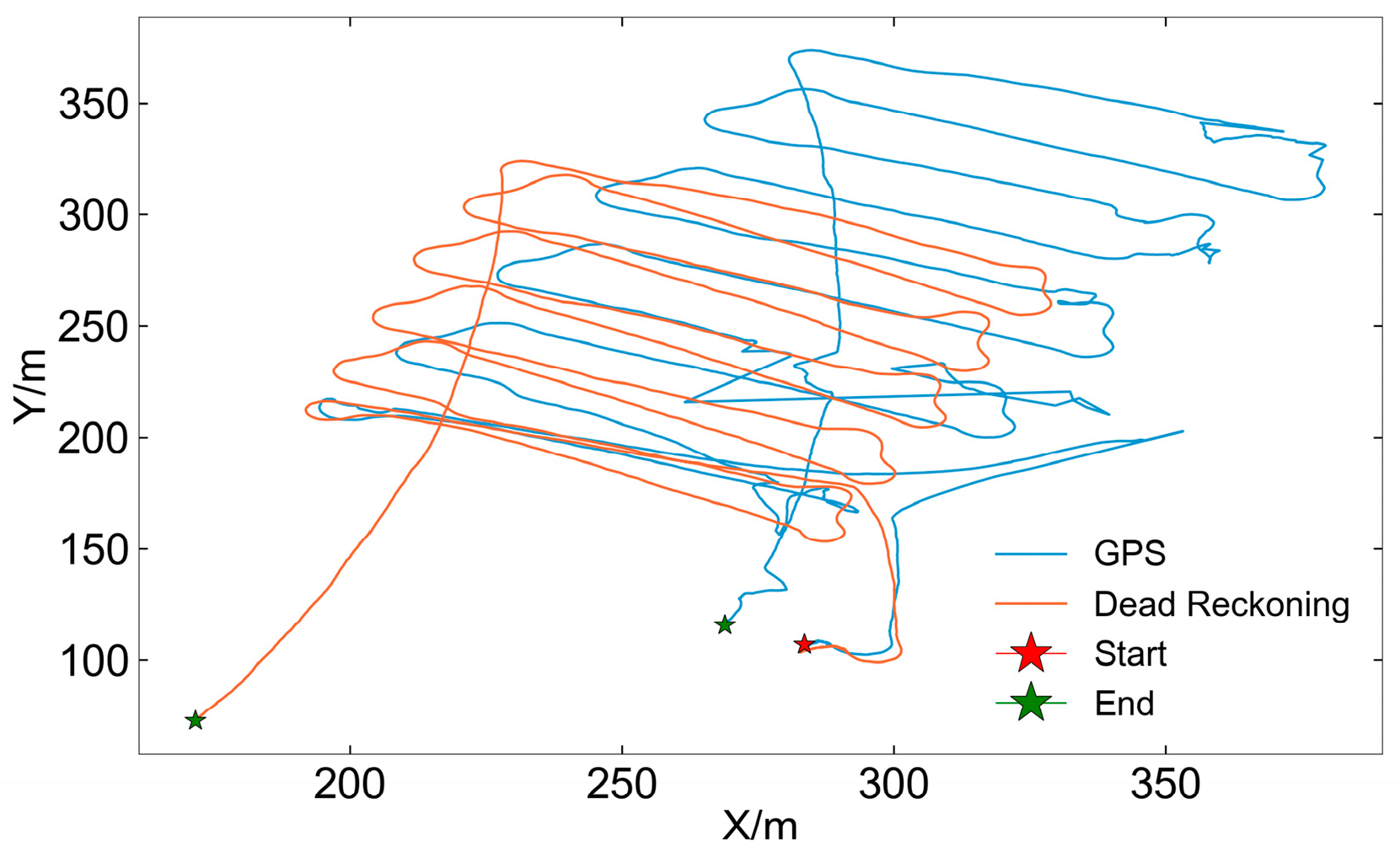
To address this issue, we further introduce a refined approach for adjusting the number of ensemble members based on the credibility of the filtering outputs. This approach establishes a threshold and calculates the Euclidean distance between the dead reckoning positioning data and GPS data, as specified in Equation (29).

$$d=\sqrt{{(x_{DR}-x_{GPS})}^2+{(y_{DR}-y_{GPS})}^2}$$

(29)

where $(x_{DR},y_{DR})$ and $(x_{GPS},y_{GPS})$ denote the positional coordinates derived from dead reckoning and GPS measurements, respectively, and $d$ represents the Euclidean distance deviation between them. If $d$ is found to be significantly large and persists above the threshold $d_{threshold}$ for a specified duration, it indicates a substantial deviation between the dead reckoning positioning data and the GPS data. In such cases, it is necessary to increase the number of ensemble members in order to maintain algorithmic precision. Conversely, if $d$ decreases and remains below the threshold for a certain period, the method reduces the number of ensemble members. The determination of the threshold $d_{threshold}$, the increment in member numbers once this threshold is surpassed, as well as the upper limit of the increase, should be tailored to the specific requirements of the navigation task and the scale of the mission area.

5.2. Validation of Adaptive Mechanism

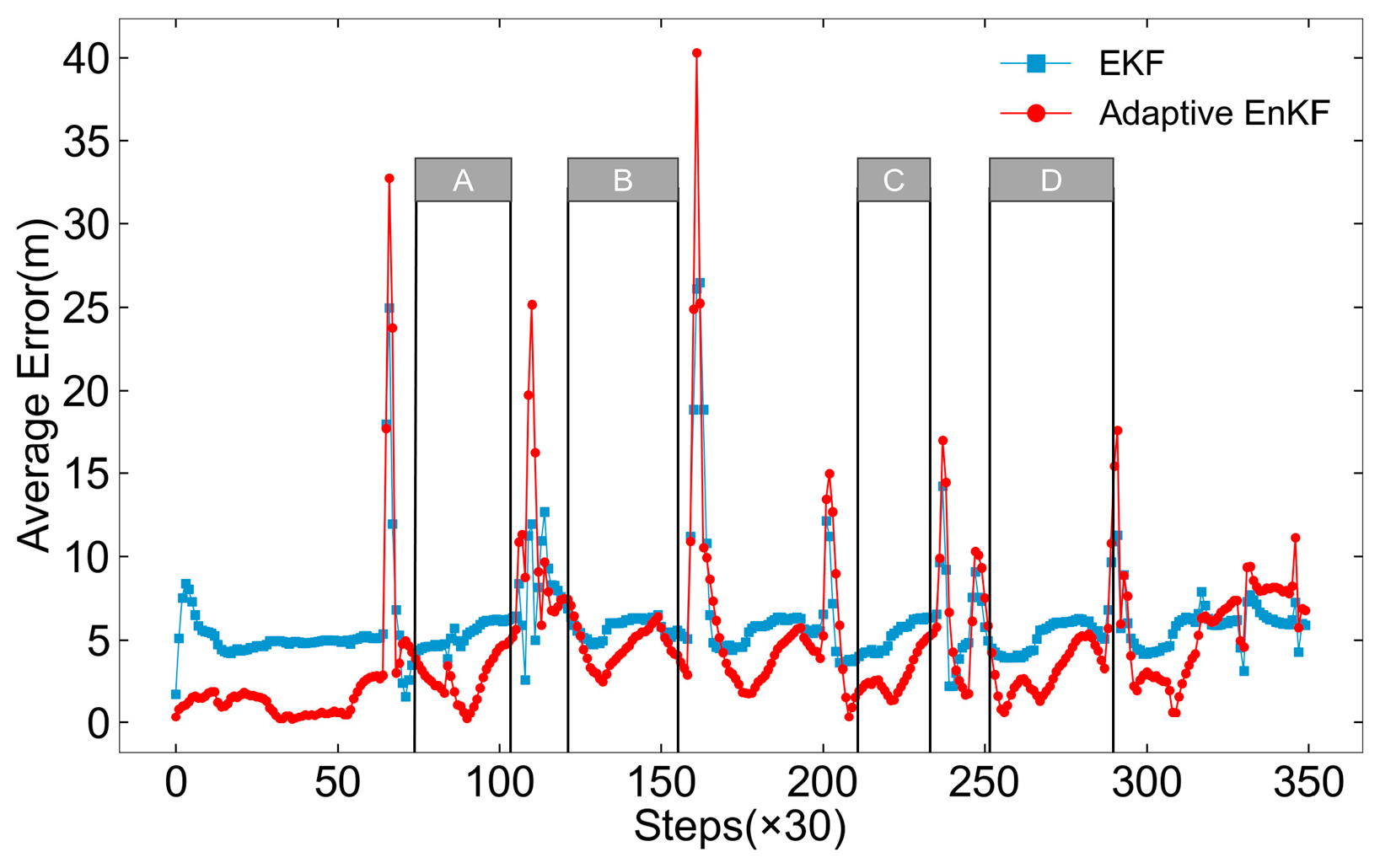
To validate the filtering performance of the EnKF algorithm enhanced with the adaptive mechanism described above, a comparative analysis is conducted between the EnKF algorithm before and after implementing this adaptive mechanism. The comparative analysis involves the following four scenarios of the EnKF algorithm, each applied to filter and assess navigation data:

A. EnKF with a constant ensemble size of 250;

B. EnKF adaptively adjusting the ensemble size based on both the smoothness of the filtered trajectory and the credibility of the filtering outputs;

C. EnKF adaptively adjusting the ensemble size solely based on the smoothness of the filtered trajectory;

D. EnKF adaptively adjusting the ensemble size solely based on the credibility of the filtering results.

In all four scenarios, the initial sample size of the ensemble is set to 250. The adaptive mechanism statistically evaluates the filtering results every 20 sampling points and adjusts the ensemble size based on the two independent criteria. By statistically analyzing the angular distribution of smoothed navigation data and considering the size and characteristics of the field test mission area, we have established a general range for setting the thresholds and parameters of the adaptive mechanism. Through multiple iterative tests and parameter optimization, the parameters of the adaptive mechanism are finalized. For the part of the adaptive mechanism using filtering smoothness as a criterion, thresholds of 170° and 150° are set as the upper and lower bounds, respectively. The ensemble size adjustment range is ±150 with an adjustment step size of 30. For the part of the adaptive mechanism using the deviation $d$ between dead reckoning and GPS data as a criterion, thresholds of 30 m and 100 m are set as the lower and upper bounds, respectively. And the ensemble size adjustment range is from 0 to 100, with a step size of 10. If the corresponding criterion exceeds the specified thresholds, the number of ensemble members is adjusted according to the relevant parameters to balance the algorithm’s performance in terms of computational efficiency and filtering stability. It should be noted that the adaptive threshold and sample size adjustment scheme used in this section are optimized results specifically tailored to the current experimental conditions, derived through repeated trials, rather than fixed, universally optimal values. Aside from the variable ensemble size, the other parameters within the algorithm remain unchanged across the scenarios.

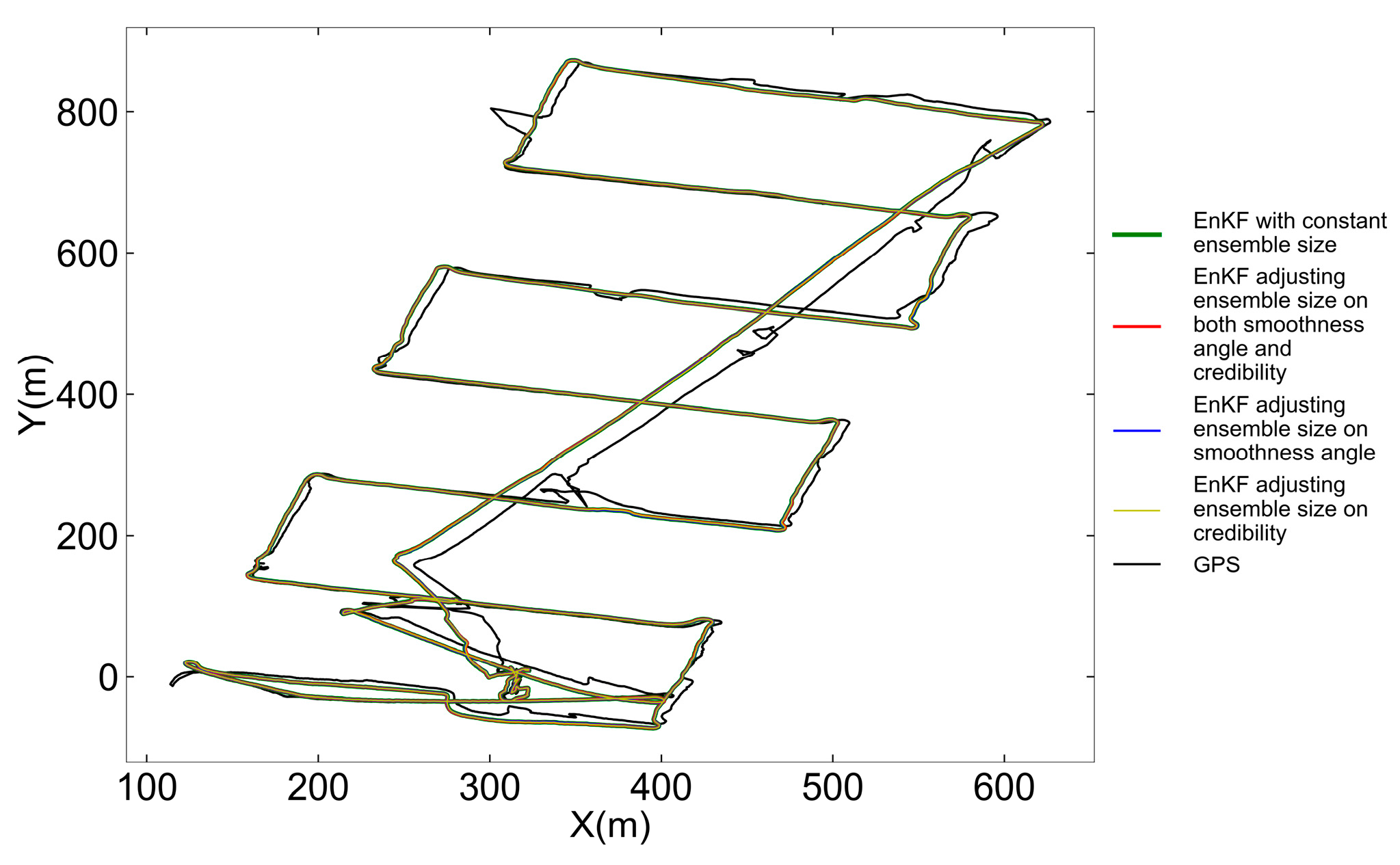
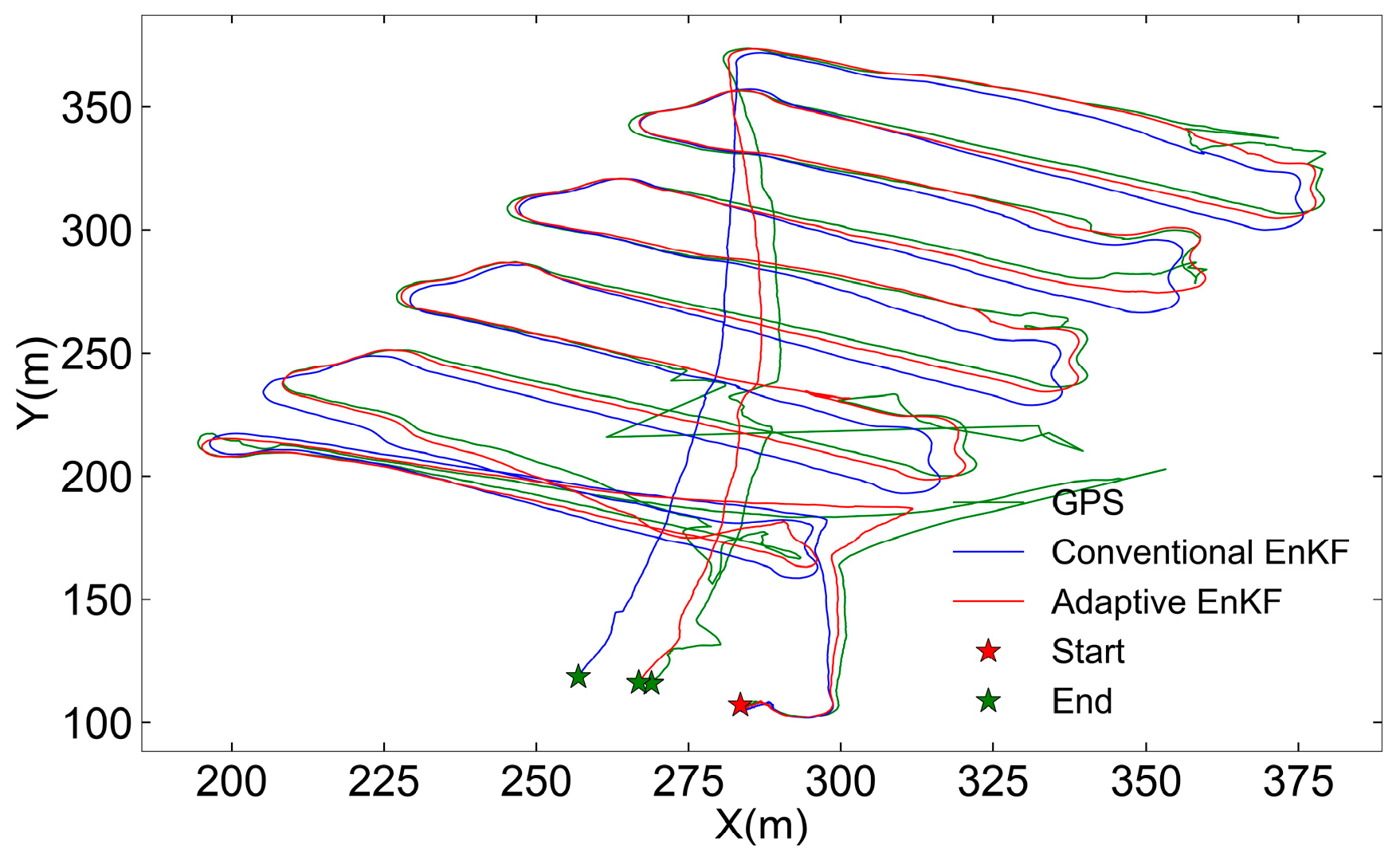
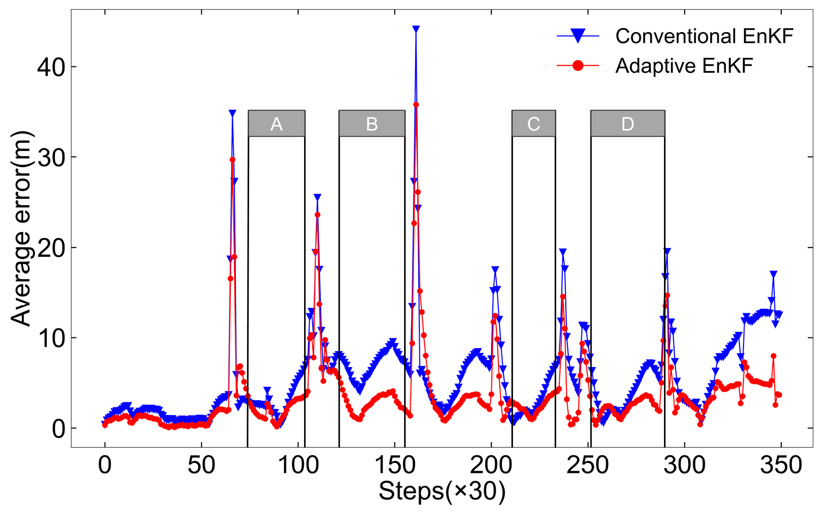
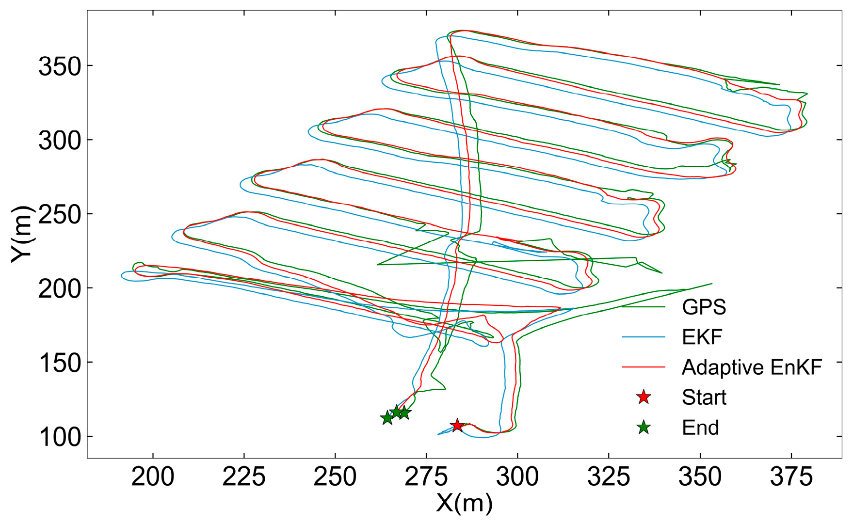
To compare the filtering performance of the four scenarios mentioned above, a series of repeated trials utilizing AUV measurements, which encompass complex motion states, are conducted. For each filtering scenario, the AUV trajectories after filtering are presented in Figure 15. The filtering trajectories generated by the algorithm under the four scenarios demonstrate a considerable degree of overlap, making it difficult to accurately assess the precision and smoothness of the algorithm across these scenarios based solely on the curves presented in Figure 15. This consistency is attributed to the parameter optimization described in Section 4, which has rendered the algorithm’s filtering effect on the navigation data both stable and reliable, leads to only minor differences in the positioning results across the scenarios.

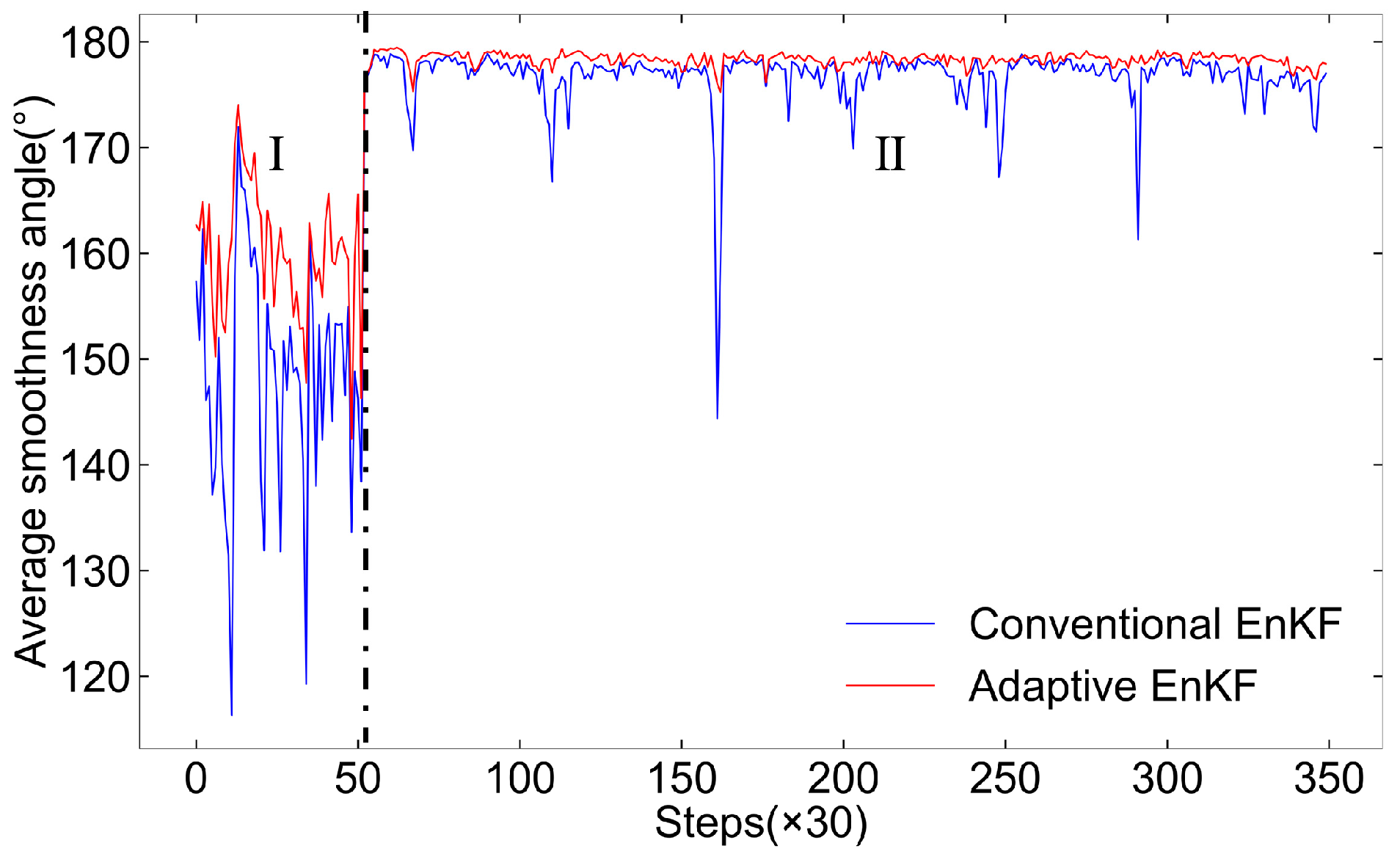
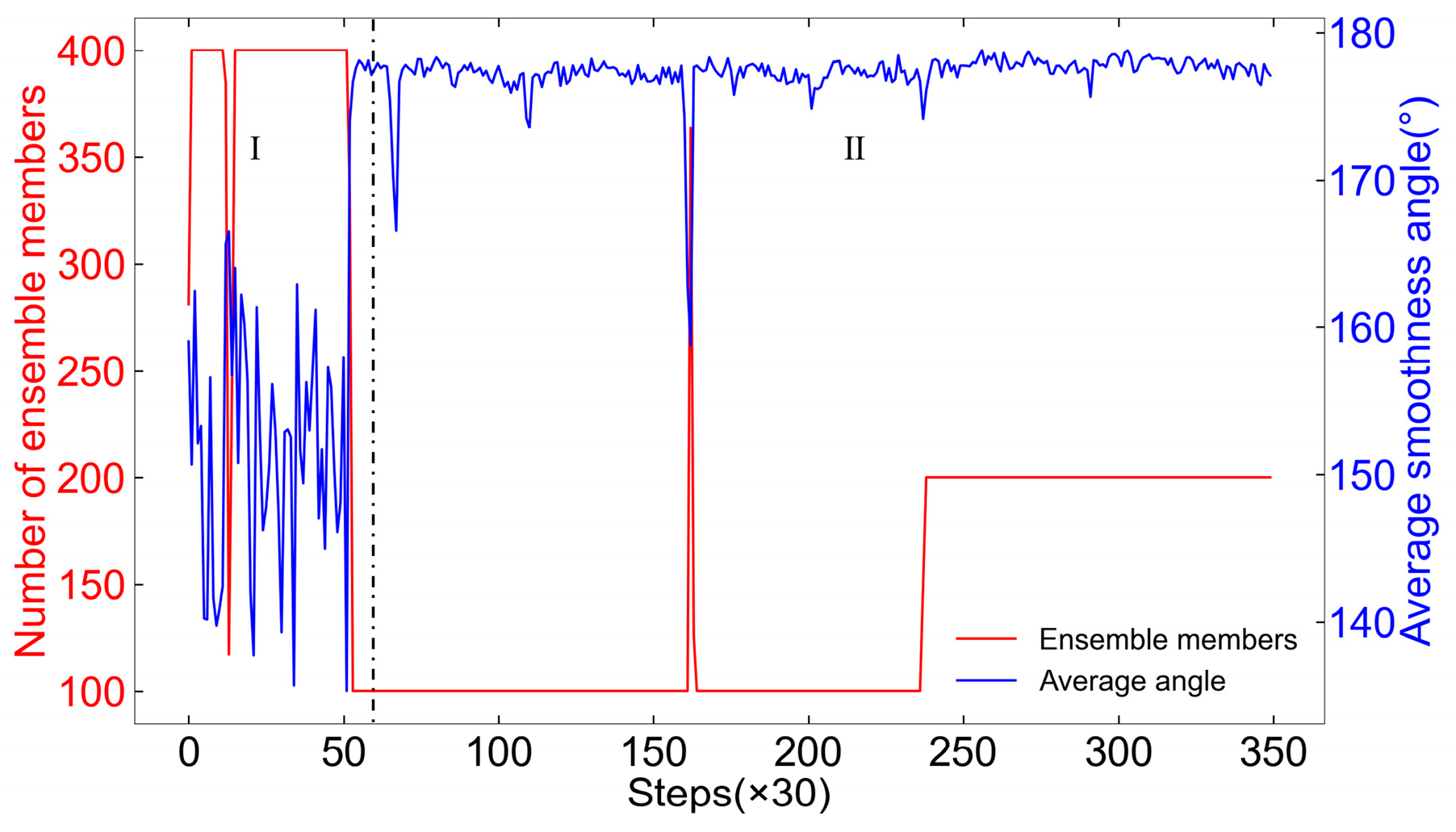
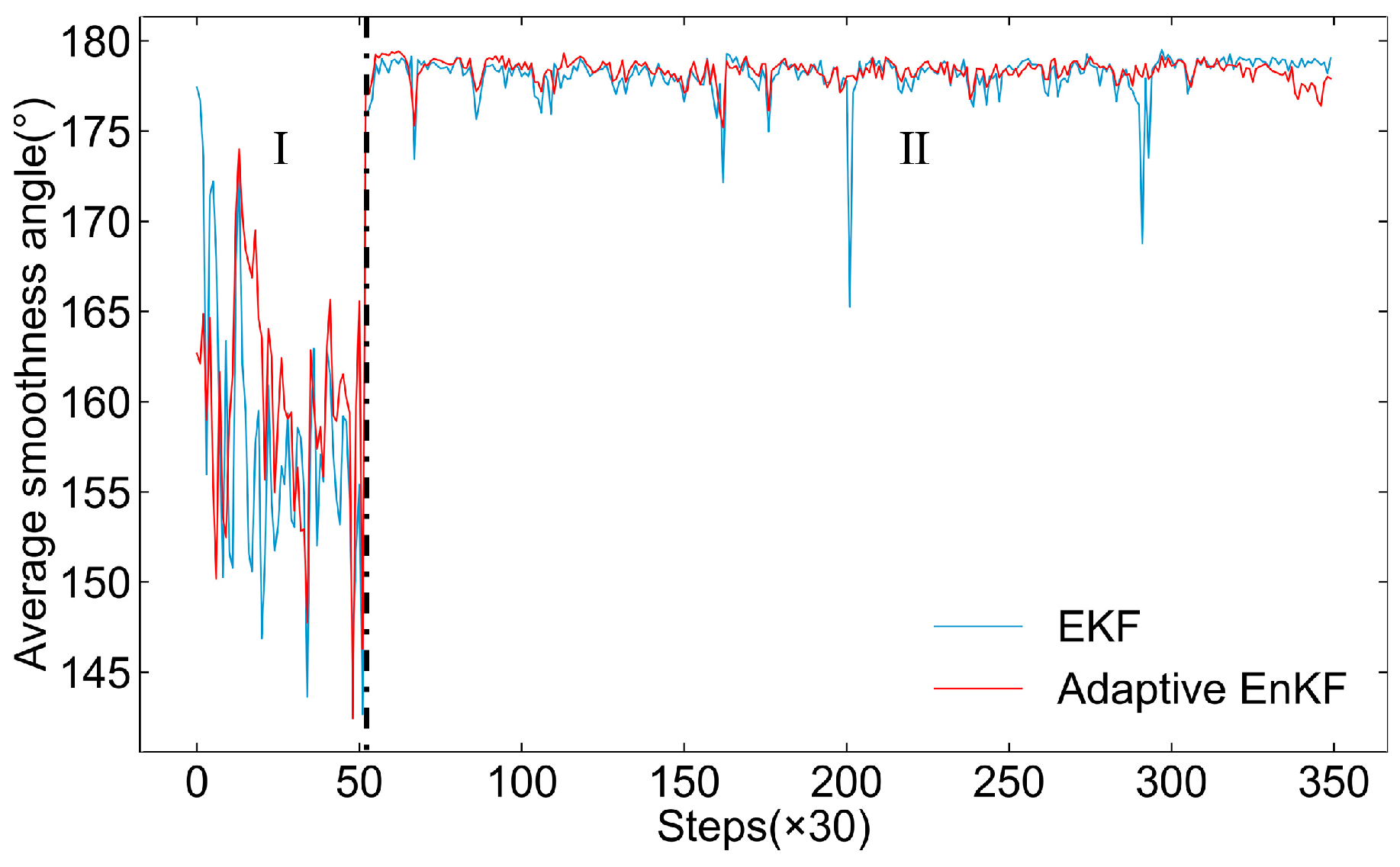
To compare the algorithm’s smoothing performance under different scenarios, Figure 16 depicts the average smoothness angle of filtered trajectories and changes in ensemble member numbers in four scenarios. The AUV trajectory is divided into three segments, I, II, and III, based on its motion state. Segment I features complex movement with frequent attitude changes and trajectory fluctuations, leading to varying filtering smoothness, as shown in Figure 16a. The red and blue curves in Figure 16b represent the EnKF algorithm scenarios that take the smoothness of the trajectory into consideration, resulting in smoother, more stable smoothness distributions. Unlike the green and yellow curves, which drop to a local minimum smoothness angle of about 138°, the red and blue curves increase by 10°, mitigating smoothness reduction.

In Segment II, AUV demonstrates a relatively steady movement, exhibiting minimal fluctuations in trajectory smoothness. Consequently, the red and blue curves in Figure 16b show a decrease in ensemble sizes, staying below the initial 250. This reduction slightly lowers the smoothness, with the red and blue curves in Figure 16a showing an average smoothness angle smaller within 3° than the green and yellow curves. This indicates that moderately reducing ensemble members during stable AUV motion has little impact on filtering smoothness.

The AUV’s movement in Segment III becomes complex again, causing frequent fluctuations in filtering smoothness, as shown in Figure 16a. The red and blue curves in Figure 16b respond by frequently adjusting the ensemble sizes. The red and yellow curves, employing an adaptive mechanism based on the filtering output credibility, increase ensemble members due to growing discrepancies between dead reckoning and GPS positioning. The red curve, employing both adaptive mechanisms, effectively limits low smoothness levels, showing relatively optimal performance in Figure 16a with a local minimum smoothness improvement of up to 5° compared to the other scenarios.

Furthermore, the algorithm’s operational efficiency in the four scenarios is analyzed, with average runtime data presented in

Table 1. Average computational time per iteration for algorithm across four scenarios.

	EnKF with a Constant Ensemble Size (Green Curve)	Adaptive EnKF Based on Both Smoothness and Credibility of Filtering Outputs (Red Curve)	Adaptive EnKF Based on Smoothness of Filtering Results (Blue Curve)	Adaptive EnKF Based on Credibility of Filtering Outputs (Yellow Curve)
Total time (s)	39.0735 s	36.0798 s	35.7675 s	39.4438 s
Average runtime per iteration (s)	0.0012785 s	0.0011784 s	0.0011683 s	0.0012895 s
Relative time consumption	100%	92.17%	91.38%	100.86%

. The scenario that adjusts ensemble size based on filtering smoothness, particularly during smooth AUV movement, operates significantly more efficiently than those without this adaptive mechanism. In contrast, the scenario that adapts based on the credibility of filtering outputs, increasing ensemble sizes to counter navigation errors, shows a slight increase in runtime. The red curve scenario, which adapts based on both smoothness and credibility, accelerates the filtering process, reducing iteration time by about 10% compared to the conventional EnKF algorithm. Despite this efficiency boost as well as the improvement of filtering smoothness shown in Figure 14, there is no noticeable increase in positioning error. In practical underwater operations, as the duration of the task increases, the improvements in filtering accuracy, smoothness, and speed are expected to have an even greater impact on enhancing the AUV’s positioning performance.

In conclusion, the EnKF with an adaptive mechanism for adjusting ensemble sizes based on filtering smoothness and output credibility demonstrates superior efficiency and smoothness, confirming that the proposed adaptive EnKF is better suited for real-world observational requirements and outperforms the conventional EnKF in real-time navigation. The algorithm’s operational flowchart incorporating the adaptive mechanism is shown in Figure 17. The mechanism adjusts the number of ensemble members $n$ according to deviation $d$ between dead reckoning and GPS positioning data, as well as the average smoothness angle $\theta$ of the filtered trajectory points. This adjustment controls the number of members included in the generated vector ensembles $X_k$ and $Z_k$ thereby influencing the performance of the subsequent EnKF filtering operations. The filtered result $x_k^{*}$ is the final optimized estimation of AUV position at time $k$.

6. Comparison of Filtering Performance

In Section 4 and Section 5, comparative analysis is conducted using field data to optimize the filtering parameters and to incorporate and verify the adaptive mechanism of the proposed EnKF algorithm, respectively. In this section, a new set of field data will be utilized to compare the performance of the adaptive EnKF algorithm against the conventional EnKF and EKF algorithms thereby further validating its effectiveness.

Figure 18 presents the GPS positioning and dead reckoning trajectories based on the new set of AUV field data. The AUV moves continuously on the water surface. On the one hand, the GPS data, significantly affected by environmental factors, exhibits considerable instability and fluctuations with notable deviations in certain areas. On the other hand, the repeated attitude changes in the AUV during continuous movement cause the DVL-based dead reckoning information to accumulate substantial positioning errors. Therefore, a combined navigation algorithm is required to integrate and correct these two data sources, providing more accurate, stable, and smooth AUV positioning results.

For the comparative analysis of filtering performance, both the conventional EnKF and the EKF algorithms used for comparison have optimized parameters. To highlight the differences, the conventional EnKF algorithm without the adaptive mechanism employs a standard Gaussian distribution for ensemble member generation.

6.1. Comparison with Conventional EnKF

The adaptive EnKF algorithm optimized in Section 5 and the conventional EnKF algorithm are each used to filter and optimize the aforementioned AUV navigation data. The resulting filtered trajectories are shown in Figure 19. It shows that the filtering trends of the two EnKF algorithms are similar, both achieving greater smoothness compared to the GPS positioning data. But notably, the filtering results of the adaptive EnKF algorithm are more closely aligned with the GPS data in Figure 19.

Figure 20 presents a comparison of the average smoothness angle distributions after filtering by the two EnKF algorithms. The comparison illustrates that the adaptive EnKF algorithm generally achieves a slightly higher average smoothness angle than the conventional EnKF algorithm and displays significantly smaller fluctuations in smoothness. With computation, the average angle of trajectory points filtered by the conventional EnKF algorithm is found to be 172.52° with a RMSE of 18.81°. The adaptive EnKF algorithm yields an average angle of 175.88° and a RMSE of 10.16°.

In Segment I of Figure 20 (within the first 60 time steps on the $x$-axis), the conventional EnKF algorithm shows an average smoothness angle of 152.20° with an RMSE of 17.14°, while the adaptive EnKF achieves a higher average smoothness angle of 163.52° and a lower RMSE of 13.81°, representing an improvement of approximately 11° in smoothness angle compared to the conventional algorithm. This indicates that the adaptive EnKF better suppresses smoothness variations, maintaining stability when the conventional EnKF’s smoothness drops. In Segment II, during stable AUV movement, the adaptive EnKF maintains a higher smoothness angle of 178.44° with a lower RMSE of 3.28°, compared to the conventional EnKF’s 176.72° and RMSE of 7.76°. It demonstrates that the adaptive EnKF not only improves the average smoothness angle, but also reduces the RMSE, which represents the fluctuation in the smoothness angle, by more than 50%. Overall, the adaptive EnKF consistently delivers higher smoothness and lower RMSE across different motion conditions (either turning or straight running), demonstrating superior filtering stability.

Figure 21 highlights how the number of ensemble members varies with smoothness in the adaptive EnKF filtering process, demonstrating the effectiveness of the adaptive mechanism. The mechanism promptly adjusts ensemble member counts based on smoothness variations, initially using a higher number of members during the initial phases of AUV motion, then reducing the number in later phases while responding to minor smoothness fluctuations. This efficient adjustment helps conserve computational resources. Overall, the adaptive EnKF algorithm enhances both filtering smoothness and stability compared to the conventional EnKF, proving the adaptive mechanism’s effectiveness.

To compare the positioning accuracy of the algorithms, GPS data are used as a reference to calculate the average Euclidean distance between the filtering results and GPS positions. To better illustrate positioning trends, this distance is computed every 30 sampling points. However, due to environmental disturbances during the AUV trial, some GPS data are unstable. Therefore, four stable segments of GPS data are selected for comparison, as shown in Figure 22. Both EnKF algorithms show similar trends, but the adaptive EnKF (red curve) consistently achieves lower errors than the conventional EnKF (blue curve), demonstrating better error control. In the four segments, the average positioning deviations for the conventional and adaptive EnKF algorithms are 4.28 m and 2.98 m, respectively, with RMSE values of 2.54 m and 2.03 m. These results indicate that the adaptive EnKF provides superior accuracy in positioning, reducing the average positioning error by 30% compared to the conventional EnKF.

Finally, the filtering performance data of the two EnKF algorithms are summarized and compared in

Table 2. Summary of the filtering performance of the conventional EnKF and the adaptive EnKF algorithms.

		Conventional EnKF		Adaptive EnKF
		Average	RMSE	Average	RMSE
Smoothness angle	Total	172.52°	18.81°	175.88°	10.16°
	Segment I	152.20°	17.14°	163.52°	13.81°
	Segment II	176.72°	7.76°	178.44°	3.28°
Absolute Error		4.28 m	2.54 m	2.98 m	2.03 m

. In conjunction with the aforementioned analysis of filtering smoothness and accuracy, the adaptive EnKF algorithm is capable of reducing fluctuations in positioning error without compromising the filtering smoothness. Consequently, the adaptive EnKF algorithm demonstrates superior performance in terms of positioning accuracy, stability, and filtering smoothness in comparison to the conventional EnKF algorithm.

6.2. Comparison with EKF

In this subsection, the filtered results of the adaptive EnKF algorithm are compared with the ones of the EKF algorithm. The filtered trajectories are presented in Figure 23. The figure shows that the EKF also exhibits satisfactory filtering performance.

Figure 24 compares the trajectory smoothness curves after filtering with both the EKF and adaptive EnKF algorithms. The adaptive EnKF shows a higher overall average smoothness angle than EKF, but with slightly larger fluctuations in some regions. The overall average smoothness angle for the EKF is 175.09° with the RMSE of 13.13°, while the adaptive EnKF’s values are 175.88° and 10.16°, respectively. In Segment I, where AUV movement is complex, the EKF achieves an average angle of 160.47° with an RMSE of 12.15°, whereas the adaptive EnKF shows an average angle of 163.52° and a higher RMSE of 13.81°. This indicates that, during the segment of frequent and complex changes in the AUV’s motion, the adaptive EnKF maintains an overall higher filtering smoothness performance compared to EKF, despite showing relatively higher RMSE values and greater smoothness fluctuations in Segment I. Such fluctuations stem from the adaptive EnKF algorithm’s response and adjustments to the complex motion states at this segment. However, as shown in Figure 24, the filtering smoothness angle of the adaptive EnKF generally remains above that of EKF, consistently exhibiting better smoothness performance despite the larger fluctuations. In the relatively stable middle and later stages of the motion trajectory, represented by Segment II in Figure 24, the adaptive EnKF algorithm demonstrates its ability to resist minor disturbances that could affect filtering smoothness, maintaining a high level of smoothness with minimal fluctuations. The average smoothness and the stability of the proposed algorithm are comparable to those of EKF.

Regarding filtering smoothness, the adaptive EnKF algorithm generally performs better than EKF, especially when the motion state of AUV is varying obviously. Conversely, when the motion state is relatively stable, the smoothness of the adaptive EnKF and EKF filtered trajectories seems similar, and both algorithms exhibit good stability.

To further compare the positioning accuracy of the algorithms, the position deviations between the EKF and the adaptive EnKF filtering results and the GPS positioning data are given in Figure 25. In the figure, the position deviation of both filtering algorithms remains relatively stable within the four selected segments, maintaining errors within a low range. The average position deviation of the EKF across the four segments, represented by the blue curve in Figure 25, is 5.35 m, with an RMSE of 0.88 m, while the adaptive EnKF, represented by the red curve, is 2.98 m and 2.03 m, reducing the average positioning error by 44% compared to the EKF. Although the adaptive EnKF shows a higher value of RMSE in positioning error, indicating relatively larger fluctuations in filtering error, this also reflects, to some extent, the adaptive EnKF’s adjustments to the inherent fluctuations in GPS positioning data. Nonetheless, the adaptive EnKF consistently exhibits superior positioning accuracy across different segments, as shown in Figure 25.

The summary and comparison of the filtering performance data for the adaptive EnKF and EKF algorithms are presented in

Table 3. Summary and comparison of the mean and RMSE of the filtering performance of the conventional EnKF and the adaptive EnKF.

		Adaptive EnKF		EKF
		Average	RMSE	Average	RMSE
Smoothness angle of the trajectory	Total	175.88°	10.16°	175.09°	13.13°
	0–60 steps (×30)	163.52°	13.81°	160.47°	12.15°
	After 60 steps (×30)	178.44°	3.28°	178.12°	4.97°
Absolute error		2.98 m	2.03 m	5.35 m	0.88 m
Average runtime per iteration		0.001178 s		0.000783 s

. Overall, the proposed adaptive EnKF algorithm demonstrates superior performance in terms of positioning accuracy and filtering smoothness compared to the EKF. Table 3 also includes the average runtime per iteration for each algorithm. The EKF shows a clear advantage in computational speed due to its simpler and faster processing steps, with an average computation time of approximately 0.000783 s per iteration—33.5% faster than the adaptive EnKF’s 0.001178 s. However, since the field trial data used in this study has a sampling interval of approximately 0.2 s, the computational speeds of both algorithms on the current hardware platform are more than sufficient to meet the real-time data processing requirements.

6.3. Discussion

By comparing the results presented in Table 2 and Table 3, we can summarize the filtering performance of the three algorithms: the EKF, the conventional EnKF, and the adaptive EnKF. With regard to positioning accuracy, all of them perform well, with the adaptive EnKF showing the most optimal performance by preventing error divergence and maintaining stable errors. In terms of filtering smoothness, the conventional EnKF shows inherent instability and fluctuations due to its reliance on the Monte Carlo method for ensemble state reconstruction. Consequently, its filtering smoothness is generally inferior to that of the EKF, particularly under complex AUV motion conditions. However, the adaptive EnKF, which leverages adaptive mechanism and a Laplace distribution-based vector ensemble generation method, achieves filtering smoothness and stability comparable to the EKF algorithm under stable motion conditions, and also demonstrates a superior overall performance in complex AUV motion conditions than EKF. This advantage becomes even more pronounced when the system operates in complex marine environments. In comparison to the EKF and conventional EnKF, the adaptive EnKF is better suited to address the potential challenges posed by various non-Gaussian noises that may emerge in real underwater settings and impede the accuracy of system observations.

7. Conclusions

This study proposes an enhanced adaptive EnKF algorithm for handling multi-sensor data fusion in AUV integrated navigation systems to optimize positioning accuracy. Based on the conventional EnKF algorithm, we introduced a Laplace distribution for state approximation, which improves the algorithm’s stability in real-world environments. We defined an average smoothness angle metric to evaluate the smoothness of the filtering trajectory. And we further incorporated an adaptive mechanism to dynamically adjust the performance of the algorithm by regulating the number of vector ensemble members in the algorithm. Using field tests to obtain AUV navigation data, we optimized the algorithm’s parameters and validated its performance by comparing it with the conventional EnKF and EKF.

After optimizing the core parameters, we evaluated the effectiveness of the adaptive mechanism in further enhancing the smoothness performance and computational efficiency by comparing four different EnKF scenarios. The EnKF with a fully adaptive mechanism was able to reduce runtime by about 10% compared to the conventional EnKF, while maintaining similar performance in terms of positioning accuracy and filtering smoothness. Based on post-processing results from field test AUV navigation data, the adaptive EnKF demonstrated significant advantages in both positioning accuracy and filtering smoothness. Compared to the EKF, the adaptive EnKF reduced the average positioning error by 44%, and by 30% compared to the conventional EnKF. Under complex AUV motion conditions, the adaptive EnKF showed a slightly higher average smoothness angle than the EKF, and an 11° improvement over the conventional EnKF, along with notable stability.

Given that the current adaptive mechanism only adjusts the number of ensemble members in the EnKF algorithm, future research will focus on expanding the types of parameters that can be dynamically adjusted. Additionally, we plan to incorporate more sources of real-world navigation data to further enhance the algorithm’s overall performance. Furthermore, our proposed algorithm will be implemented on our AUV platform for field trials to verify its practical applicability in specific underwater task scenarios.

References

1. Yuh, J. Design and Control of Autonomous Underwater Robots: A Survey. Auton. Robot. 2000, 8, 7–24. [Google Scholar] [CrossRef]
2. Leonard, J.J.; Bahr, A. Autonomous Underwater Vehicle Navigation. In Springer Handbook of Ocean Engineering, 1st ed.; Dhanak, M.R., Xiros, N.I., Eds.; Springer International Publishing: Cham, Switzerland, 2016; pp. 341–358. [Google Scholar] [CrossRef]
3. Mu, X.; He, B.; Wu, S.; Zhang, X.; Song, Y.; Yan, T. A Practical INS/GPS/DVL/PS Integrated Navigation Algorithm and Its Application on Autonomous Underwater Vehicle. Appl. Ocean Res. 2020, 106, 102441. [Google Scholar] [CrossRef]
4. Sahoo, A.; Dwivedy, S.K.; Robi, P.S. Advancements in the Field of Autonomous Underwater Vehicle. Ocean Eng. 2019, 181, 145–160. [Google Scholar] [CrossRef]
5. Wynn, R.B.; Huvenne, V.A.I.; Bas, T.P.; McPhail, S.D.; White, D.; Murton, B.J.; Harris, J.; Bett, B.J.; Tyler, P.A. Autonomous Underwater Vehicles (AUVs): Their Past, Present and Future Contributions to the Advancement of Marine Geoscience. Mar. Geol. 2014, 352, 451–468. [Google Scholar] [CrossRef]
6. Paglia, J.G.; Wyman, W.F. DARPA’S Autonomous Minehunting and Mapping Technologies (AMMT) Program: An Overview. In Proceedings of the OCEANS 96 MTS/IEEE Conference: The Coastal Ocean—Prospects for the 21st Century, Fort Lauderdale, FL, USA, 23–26 September 1996; IEEE: Fort Lauderdale, FL, USA, 1996; pp. 794–799. [Google Scholar] [CrossRef]
7. Larsen, M.B. High Performance Autonomous Underwater Navigation: Experimental Results. Hydro Int. 2002, 6, 6–9. [Google Scholar]
8. Li, Y.P.; Feng, X.S. Application of 6000 m Autonomous Underwater Robots “CR-01” in the Investigation of Manganese Nodules in the Pacific Ocean. High Technol. Lett. 2001, 1, 85–87. [Google Scholar]
9. Stutters, L.; Liu, H.; Tiltman, C.; Brown, D. Navigation Technologies for Autonomous Underwater Vehicles. IEEE Trans. Syst. Man Cybern. C 2008, 38, 581–589. [Google Scholar] [CrossRef]
10. Zhang, B.; Ji, D.; Liu, S.; Zhu, X.; Xu, W. Autonomous Underwater Vehicle Navigation: A Review. Ocean Eng. 2023, 273, 113861. [Google Scholar] [CrossRef]
11. Paull, L.; Saeedi, S.; Seto, M.; Li, H. AUV Navigation and Localization: A Review. IEEE J. Ocean. Eng. 2014, 39, 131–149. [Google Scholar] [CrossRef]
12. Silva, D.C.; Frutuoso, A.; Souza, L.F.; de Barros, E.A. Comparative Analysis of Innovation-Based Adaptive Kalman Filters Applied to AUVs Navigation. In Proceedings of the 2022 Latin American Robotics Symposium (LARS), 2022 Brazilian Symposium on Robotics (SBR), and 2022 Workshop on Robotics in Education (WRE), São Bernardo do Campo, Brazil, 10 October 2022; pp. 31–36. [Google Scholar] [CrossRef]
13. Memon, S.A.; Son, H.; Kim, W.-G.; Khan, A.M.; Shahzad, M.; Khan, U. Tracking Multiple Autonomous Ground Vehicles Using Motion Capture System Operating in a Wireless Network. IEEE Access 2024, 12, 61780–61794. [Google Scholar] [CrossRef]
14. Memon, S.A.; Son, H.; Kim, W.-G.; Khan, A.M.; Shahzad, M.; Khan, U. Tracking Multiple Unmanned Aerial Vehicles through Occlusion in Low-Altitude Airspace. Drones 2023, 7, 241. [Google Scholar] [CrossRef]
15. Chen, R.; Li, T.; Memon, I.; Shi, Y.; Ullah, I.; Memon, S.A. Multi-Sonar Distributed Fusion for Target Detection and Tracking in Marine Environment. Sensors 2022, 22, 3335. [Google Scholar] [CrossRef] [PubMed]
16. Kalman, R.E. A New Approach to Linear Filtering and Prediction Problems. J. Basic Eng. 1960, 82, 35–45. [Google Scholar] [CrossRef]
17. Fryxell, D.; Oliveira, P.; Pascoal, A.; Silvestre, C.; Kaminer, I. Navigation, Guidance and Control of AUVs: An Application to the MARIUS Vehicle. Control Eng. Pract. 1996, 4, 401–409. [Google Scholar] [CrossRef]
18. Barfoot, T.D.; Forbes, J.R.; Yoon, D.J. Exactly Sparse Gaussian Variational Inference with Application to Derivative-Free Batch Nonlinear State Estimation. Int. J. Robot. Res. 2020, 39, 1473–1502. [Google Scholar] [CrossRef]
19. Fulton, T.F.; Cassidy, C.J. Navigation Sensor Data Fusion for the AUV Remus. Mar. Technol. SNAME News 2001, 38, 65–69. [Google Scholar] [CrossRef]
20. Crassidis, J.L. Sigma-Point Kalman Filtering for Integrated GPS and Inertial Navigation. IEEE Trans. Aerosp. Electron. Syst. 2006, 42, 750–756. [Google Scholar] [CrossRef]
21. Julier, S.J.; Uhlmann, J.K. Unscented Filtering and Nonlinear Estimation. Proc. IEEE 2004, 92, 401–422. [Google Scholar] [CrossRef]
22. Allotta, B.; Ridolfi, A.; Costanzi, R.; Monni, N.; Nuti, F.; Fenucci, D.; Mengali, G. An Unscented Kalman Filter-Based Navigation Algorithm for Autonomous Underwater Vehicles. Mechatronics 2016, 39, 185–195. [Google Scholar] [CrossRef]
23. Krauss, S.T.; Stilwell, D.J. Unscented Kalman Filtering on Manifolds for AUV Navigation—Experimental Results. In Proceedings of the OCEANS 2022, Hampton Roads, VA, USA, 10–13 October 2022; pp. 1–6. [Google Scholar] [CrossRef]
24. Arulampalam, M.S.; Maskell, S.; Gordon, N.; Clapp, T. A Tutorial on Particle Filters for Online Nonlinear/Non-Gaussian Bayesian Tracking. IEEE Trans. Signal Process. 2002, 50, 174–188. [Google Scholar] [CrossRef]
25. Shariati, H.; Moosavi, H.; Danesh, M. Application of Particle Filter Combined with Extended Kalman Filter in Model Identification of an Autonomous Underwater Vehicle Based on Experimental Data. Appl. Ocean Res. 2019, 82, 32–40. [Google Scholar] [CrossRef]
26. Donovan, G.T. Position Error Correction for an Autonomous Underwater Vehicle Inertial Navigation System (INS) Using a Particle Filter. IEEE J. Ocean. Eng. 2012, 37, 431–445. [Google Scholar] [CrossRef]
27. Liu, C.; Xue, J. The Ensemble Kalman Filter Theory and Method Development. J. Trop. Meteorol. 2005, 21, 628–633. [Google Scholar]
28. Cui, B.; Zhang, J. The Improved Ensemble Kalman Filter for Multisensor Target Tracking. In Proceedings of the 2008 International Symposium on Information Science and Engineering, Shanghai, China, 20–22 December 2008; pp. 263–265. [Google Scholar] [CrossRef]
29. Pornsarayouth, S.; Wongsaisuwan, M.; Yamakita, M. An Improvement of Ensemble Kalman Filter for OOSM Tracking. IFAC Proc. Vol. 2011, 44, 12003–12008. [Google Scholar] [CrossRef]
30. Tin, N.; Apriliani, E.; Nurhadi, H. Comparison of AUV Position Estimation Using Kalman Filter, Ensemble Kalman Filter and Fuzzy Kalman Filter Algorithm in the Specified Trajectories. InPrime Indones. J. Pure Appl. Math. 2022, 4, 1–18. [Google Scholar] [CrossRef]
31. Ngatini; Apriliani, E.; Nurhadi, H. Ensemble and Fuzzy Kalman Filter for Position Estimation of an Autonomous Underwater Vehicle Based on Dynamical System of AUV Motion. Expert Syst. Appl. 2017, 68, 29–35. [Google Scholar] [CrossRef]
32. Tin, N.; Nurhadi, H. Estimasi Lintasan AUV 3 Dimensi (3D) Dengan Ensemble Kalman Filter. INOVTEK Polbeng-Seri Inform. 2018, 4, 12–21. [Google Scholar] [CrossRef]
33. Fan, S.; Zhang, X.; Zeng, G.; Cheng, X. Underwater Ice Adaptive Mapping and Reconstruction Using Autonomous Underwater Vehicles. Front. Mar. Sci. 2023, 10, 1124752. [Google Scholar] [CrossRef]
34. Miller, P.A.; Farrell, J.A.; Zhao, Y.; Djapic, V. Autonomous Underwater Vehicle Navigation. IEEE J. Ocean. Eng. 2010, 35, 663–678. [Google Scholar] [CrossRef]
35. Houtekamer, P.L.; Mitchell, H.L. Data Assimilation Using an Ensemble Kalman Filter Technique. Mon. Weather Rev. 1998, 126, 796–811. [Google Scholar] [CrossRef]
36. Aghababa, M.P.; Amrollahi, M.H.; Borjkhani, M. Application of GA, PSO, and ACO Algorithms to Path Planning of Autonomous Underwater Vehicles. J. Mar. Sci. Appl. 2012, 11, 378–386. [Google Scholar] [CrossRef]
37. Xu, C.; Xu, C.; Wu, C.; Liu, J.; Qu, D.; Xu, F. Accurate Two-Step Filtering for AUV Navigation in Large Deep-Sea Environment. Appl. Ocean Res. 2021, 115, 102821. [Google Scholar] [CrossRef]
38. Houtekamer, P.L.; Mitchell, H.L. Ensemble Kalman Filtering. Q. J. R. Meteorol. Soc. 2005, 131, 3269–3289. [Google Scholar] [CrossRef]
39. Carrillo, J.; Hoffmann, F.; Stuart, A.; Vaes, U. The Mean Field Ensemble Kalman Filter: Near-Gaussian Setting. arXiv 2022, arXiv:2212.13239. [Google Scholar] [CrossRef]
40. Kozubowski, T.J.; Nadarajah, S. Multitude of Laplace Distributions. Stat. Pap. 2010, 51, 127–148. [Google Scholar] [CrossRef]
41. Kotz, S.; Kozubowski, T.; Podgorski, K. The Laplace Distribution and Generalizations: A Revisit with Applications to Communications, Economics, Engineering, and Finance; Springer: New York, NY, USA, 2001. [Google Scholar] [CrossRef]
42. Akaike, H. A New Look at the Statistical Model Identification. IEEE Trans. Autom. Control 1974, 19, 716–723. [Google Scholar] [CrossRef]
43. Li, D.; Ji, D.; Liu, J.; Lin, Y. A Multi-Model EKF Integrated Navigation Algorithm for Deep Water AUV. Int. J. Adv. Robot. Syst. 2016, 13, 3. [Google Scholar] [CrossRef]
44. Mirzaei, M.; Hosseini, I.; Makarem, H. Attitude Determination Improvement in Accelerated Motions for Maneuvering Underwater Vehicles. Appl. Ocean Res. 2020, 104, 102355. [Google Scholar] [CrossRef]
Figure 1. Our AUV platform.
Drones 08 00711 g001
Figure 2. Longitudinal sectional view of the AUV platform structure.
Drones 08 00711 g002
Figure 3. Schematic diagram of AUV navigation system hardware connections.
Drones 08 00711 g003
Figure 4. Inertial and body-fixed coordinate frames to describe AUV motion.
Drones 08 00711 g004
Figure 5. Comparation of the function curves for the standard Gaussian distribution ( μ = 0 ,   σ = 1 ) and the standard Laplace distribution ( μ = 0 ,   b = 1 ).
Drones 08 00711 g005
Figure 6. Comparison of the probability distribution of AUV positioning trajectory deviation with two theoretical probability distribution curves, the three distributions have the same mean and standard deviation.
Drones 08 00711 g006
Figure 7. Operational flowchart of EnKF.
Drones 08 00711 g007
Figure 8. Location of test area.
Drones 08 00711 g008
Figure 9. Dead reckoning and GPS positioning trajectories during AUV field trial.
Drones 08 00711 g009
Figure 10. Partial enlarged view of AUV trajectory during turning motion with different variance values of observation vector ensemble σ p o 2 . (a) σ p o 2 = 0.1 ; (b) σ p o 2 = 1 ; (c) σ p o 2 = 10 .
Drones 08 00711 g010
Figure 11. Partial enlarged view of AUV trajectory during turning motion with different values of σ o b s 2 . (a) σ o b s 2 = 0.1 ; (b) σ o b s 2 = 1 ; (c) σ o b s 2 = 10 .
Drones 08 00711 g011
Figure 12. AUV trajectory filtered by EnKF under different measurement noise matrix perturbation variances σ v 2 .
Drones 08 00711 g012
Figure 13. Comparison of EnKF filtering trajectories with GPS and dead reckoning trajectories under different state vector ensemble. (a) Comparison of EnKF in different state vector ensemble variance values; (b) partial enlarged view by black box mark in Figure 13a.
Drones 08 00711 g013
Figure 14. Variation in runtime and average smoothness angle with number of state vector ensemble members.
Drones 08 00711 g014
Figure 15. AUV filtered trajectories in four filtering scenarios.
Drones 08 00711 g015
Figure 16. Comparison of the number of ensemble members and average filtered smoothness angle of the algorithm in four scenarios. (a) Average smoothness angles of the filtered trajectories; (b) alterations in the number of ensemble members of EnKF.
Drones 08 00711 g016
Figure 17. Operational flowchart of EnKF algorithm incorporating adaptive mechanism.
Drones 08 00711 g017
Figure 18. The navigation data used in this section. The red asterisk indicates the starting point, and the green asterisks indicate the ending points for both GPS positioning and dead reckoning.
Drones 08 00711 g018
Figure 19. Filtered trajectories by conventional EnKF and adaptive EnKF compared with GPS data.
Drones 08 00711 g019
Figure 20. Average smoothness angle distributions of conventional EnKF and adaptive EnKF.
Drones 08 00711 g020
Figure 21. The number of ensemble members varied with the smoothness angle within the adaptive EnKF filtering process.
Drones 08 00711 g021
Figure 22. Positioning deviation variations for conventional EnKF and adaptive EnKF, with segments A, B, C, and D representing relatively stable and reliable GPS positioning data.
Drones 08 00711 g022
Figure 23. Filtered trajectories by EKF and adaptive EnKF compared with GPS positioning data.
Drones 08 00711 g023
Figure 24. Average smoothness angle distributions of EKF and adaptive EnKF.
Drones 08 00711 g024
Figure 25. Positioning deviation variations for EKF and adaptive EnKF, with segments A, B, C, and D representing relatively stable and reliable GPS positioning data.
Drones 08 00711 g025