
A Hybrid ARO Algorithm and Key Point Retention Strategy Trajectory Optimization for UAV Path Planning


Abstract
1. Introduction
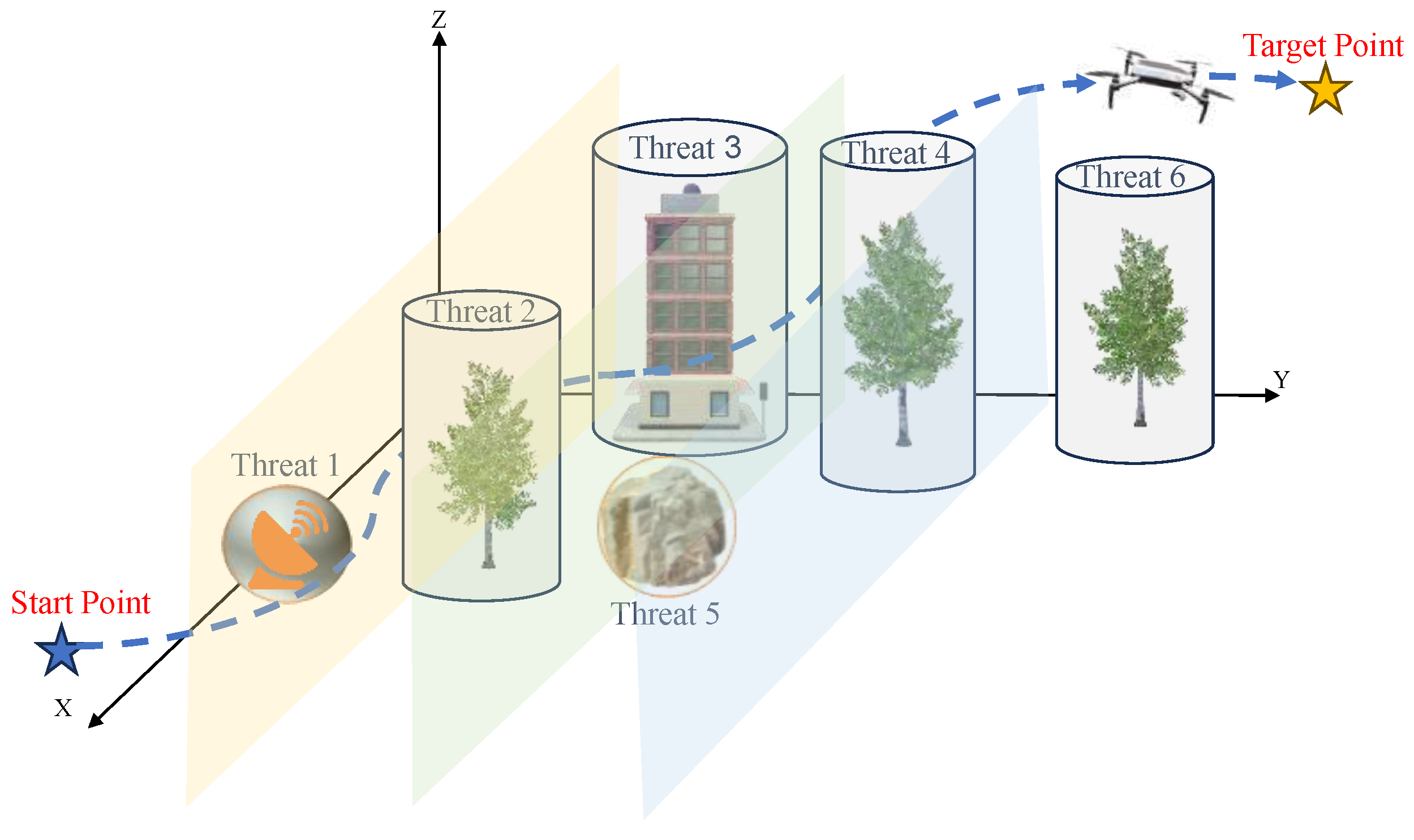
- Considering more complex and realistic scenarios, we introduce a spherical obstacle model to better replicate scene characteristics. Subsequently, we propose a hybrid multi-strategy artificial rabbits optimization (HARO+) that utilizes spherical vector coordinates to enhance the efficiency of UAV path planning in intricate environments.
- To enhance early exploration capabilities and flexibility while ensuring better candidate solutions for the development phase, we propose a dual-exploration strategy switching mechanism, balancing exploration and exploitation stages. Additionally, we introduce a population migration memory mechanism to maintain population diversity during iterations, enhancing the ability to avoid falling into local optima.
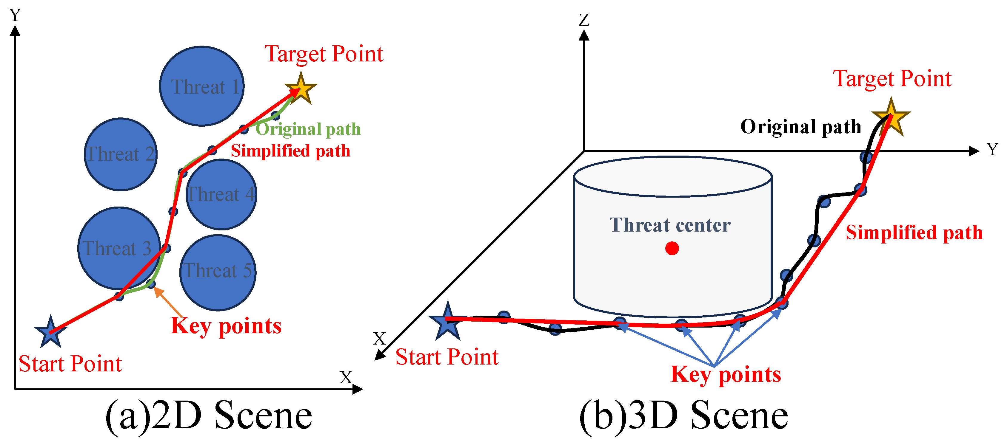
- Considering the differential treatment of preliminary paths generated by HARO based on obstacle density, we propose the key point retention trajectory optimization strategy, HARO+. This approach effectively generates safe, smooth, and cost-effective UAV flight paths in complex 2D and 3D environments.
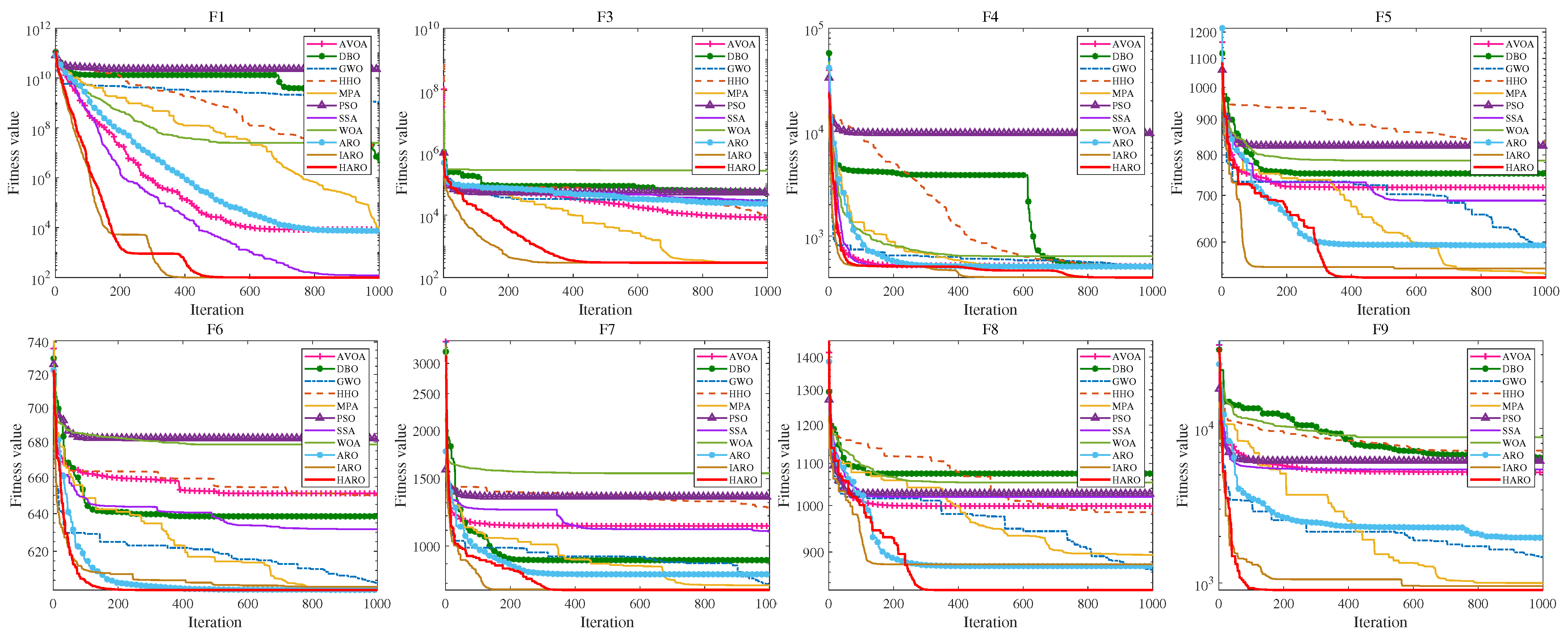
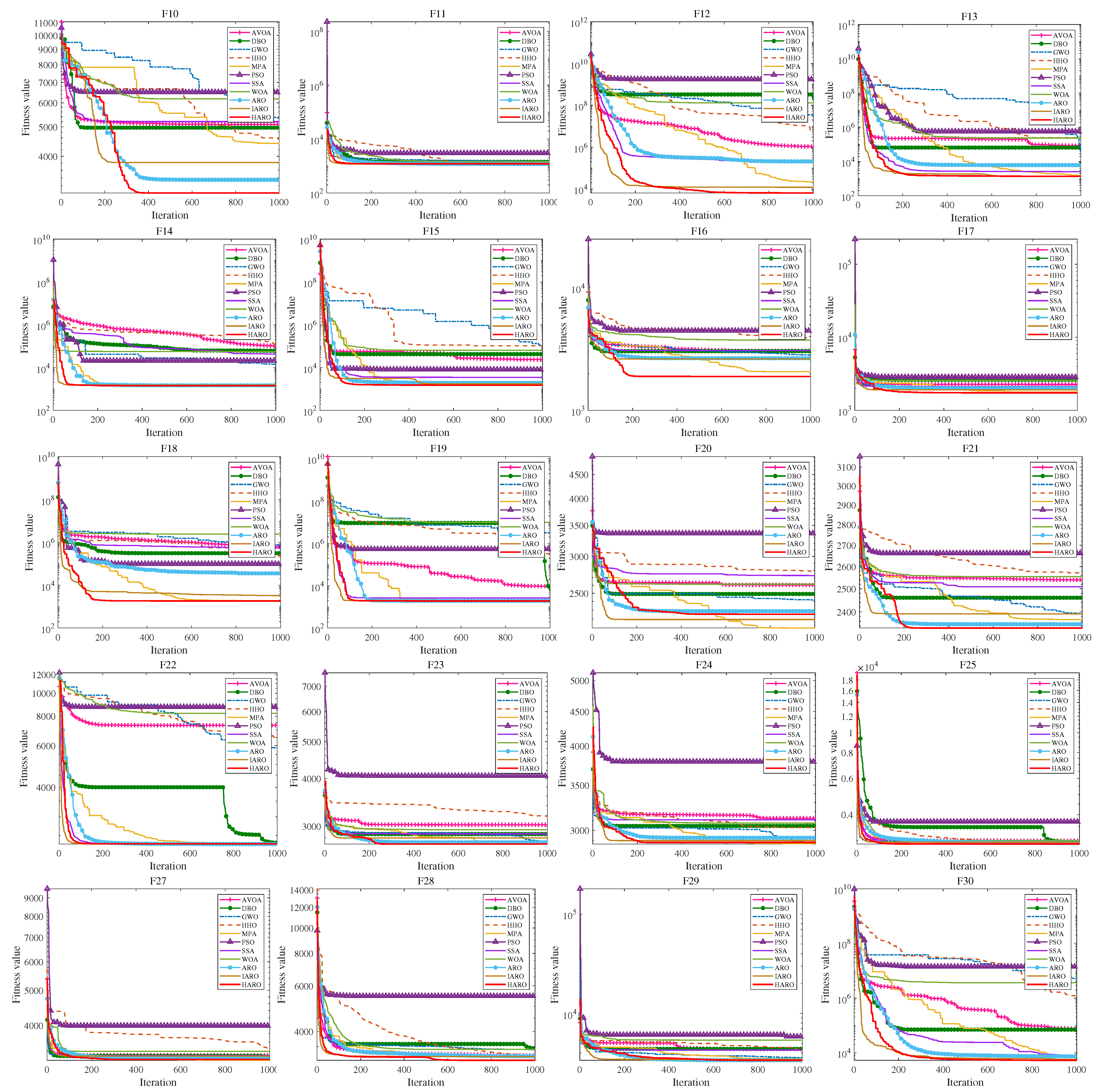
- HARO’s superior search performance is validated through comparisons with other methods using the CEC2017 test functions and various complex 2D/3D UAV flight scenarios. Additionally, the incorporation of the key point retention trajectory optimization strategy significantly reduces the fitness cost for both HARO+ and other methods (up to 4.5%), with a path point compression rate of approximately 50–80%, further validating the adaptability and compatibility of this optimization strategy in complex environments.
2. Related Work
2.1. UAV Path Planning
2.2. Artificial Rabbits Optimization Algorithm
3. Preliminaries
3.1. Definition of the UAV Path Planning Problem
3.1.1. Energy Constraint
3.1.2. Safety Constraint
3.1.3. Height Constraint
3.1.4. Attitude Angle Constraints
3.2. ARO Algorithm
3.2.1. Population Initialization
3.2.2. Detour Foraging (Exploration)
3.2.3. Random Hiding (Exploitation)
3.2.4. Energy Shrink
3.3. Douglas–Peucker Algorithm
4. The Proposed Methods
4.1. The Proposed HARO
4.1.1. Elite-Guided Exploration Strategy
4.1.2. Dual Exploration Strategy
4.1.3. Population Migration Memory Mechanism
4.1.4. The Algorithmic Process and Computational Complexity Analysis of HARO
| Algorithm 1 Pseudocode of the HARO algorithm |
| Input: The maximum iteration count T, the rabbit population size N, and the problem dimensionality D, and some other basic parameters. |
| Output: The best position of the rabbit and its corresponding fitness value |
| 1: Initialize the positions of the rabbits using Equation (14). |
| 2: whiledo |
| 3: Determine the positions and fitness values of all individuals, and implement the memory storage mechanism. Compute the energy factor F as Equation (32). |
| 4: for to N do |
| 5: Calculate the factor A by using Equation (26); |
| 6: if then |
| 7: Select a rabbit at random from other individuals; |
| 8: if then |
| 9: Perform detour foraging by using Equations (15)–(18). |
| 10: else |
| 11: Perform other exploration strategy by using Equations (28)–(30). |
| 12: end if |
| 13: else |
| 14: Create d burrows and randomly select one for hiding by using Equation (24); |
| 15: Execute random hiding in accordance with Equation (22). |
| 16: end if |
| 17: Update the position of the individual by using Equation (25) |
| 18: end for |
| 19: Accomplish memory saving, and perform the population migration mechanism by using Equations (31)–(32). |
| 20: end while. |
4.2. HARO+ Trajectory Optimization
- (1)
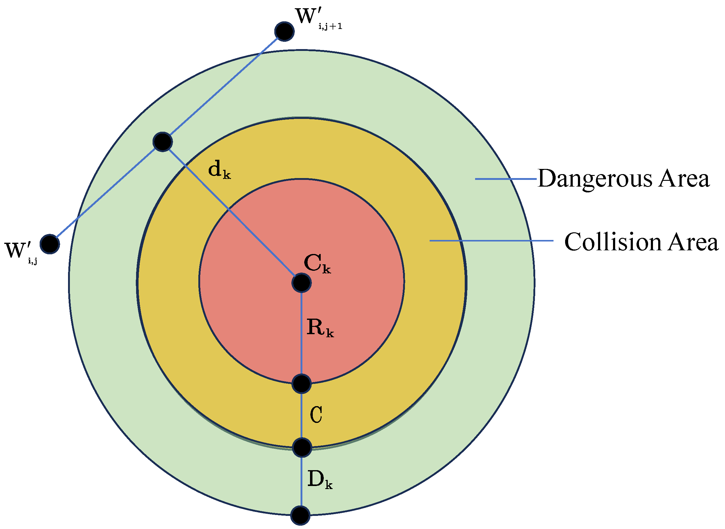
- Considering the UAV safety constraints mentioned earlier, we define path points within the danger zone as key points. Based on the actual obstacle environment, set an appropriate threshold value, D.
- (2)
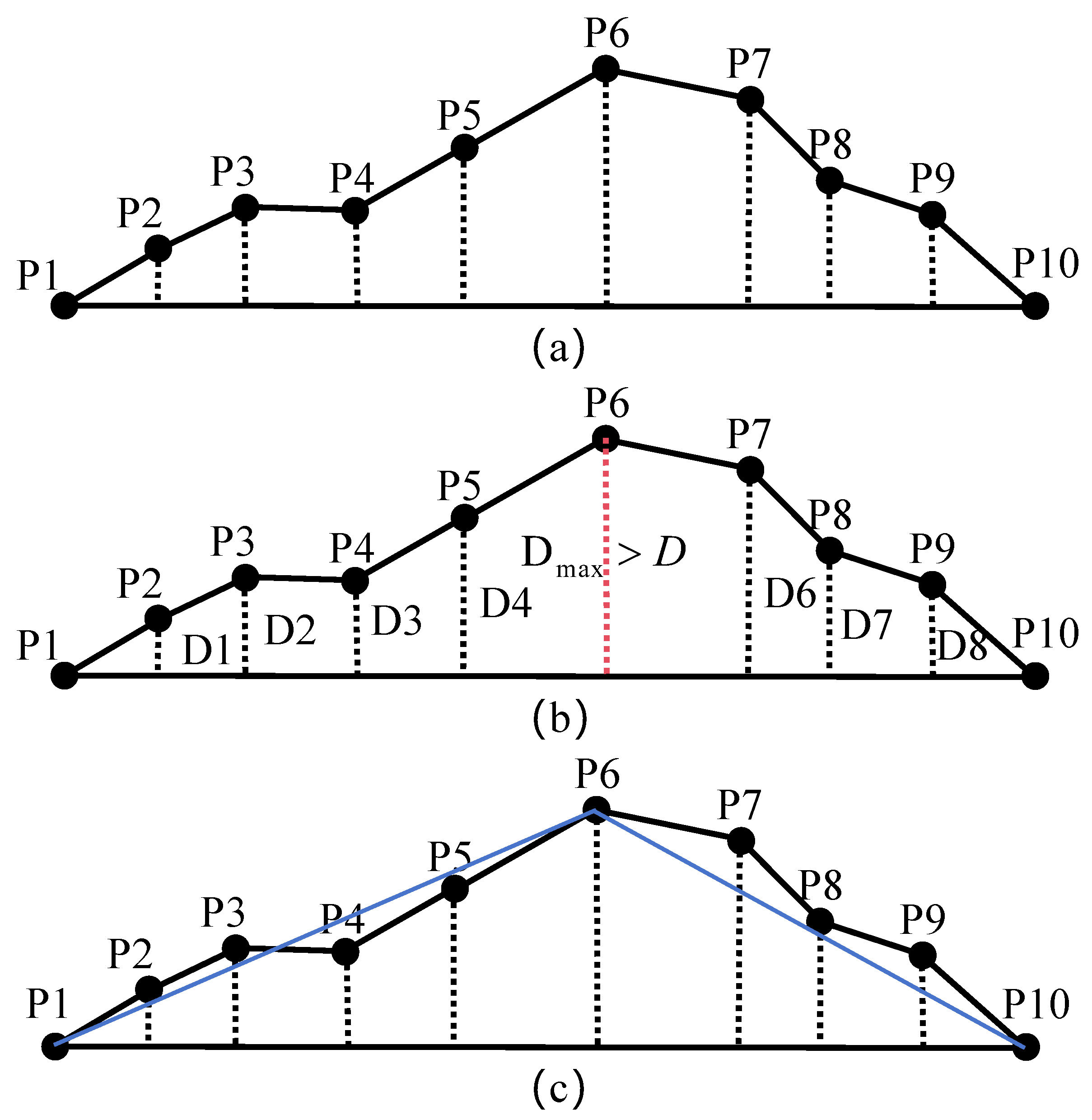
- Determine the Euclidean distance, , from each point in the flight path, P, to the centers of the obstacles it passes through. If is less than the preset danger zone radius, the path point belongs to a key point and needs to be retained; otherwise, path points outside this area can be ignored. According to the order in which the flight path passes through obstacles, these key points are sequentially stored in set , and the number of key points is denoted as n,
- (3)
- Utilize the DP algorithm to obtain the simplified set of path points . Then, traverse the key point set , adding the key point to set in order if it is not already present; otherwise, leave it unchanged. Set represents the final collection of simplified route points containing key points.
| Algorithm 2 Calculate the distance between a point to a line segment in 3D space using the Douglas–Peucker algorithm |
| Input: The point p, the starting point a of the line segment, and the ending point b of the line segment. |
| Output: The distance from the point to the line segment. |
|
5. Simulation Experiments and Result Analysis
5.1. Numerical Experiments and Analysis
5.1.1. Operating Environment Setup
5.1.2. Results and Analysis of CEC2017 Benchmark Functions
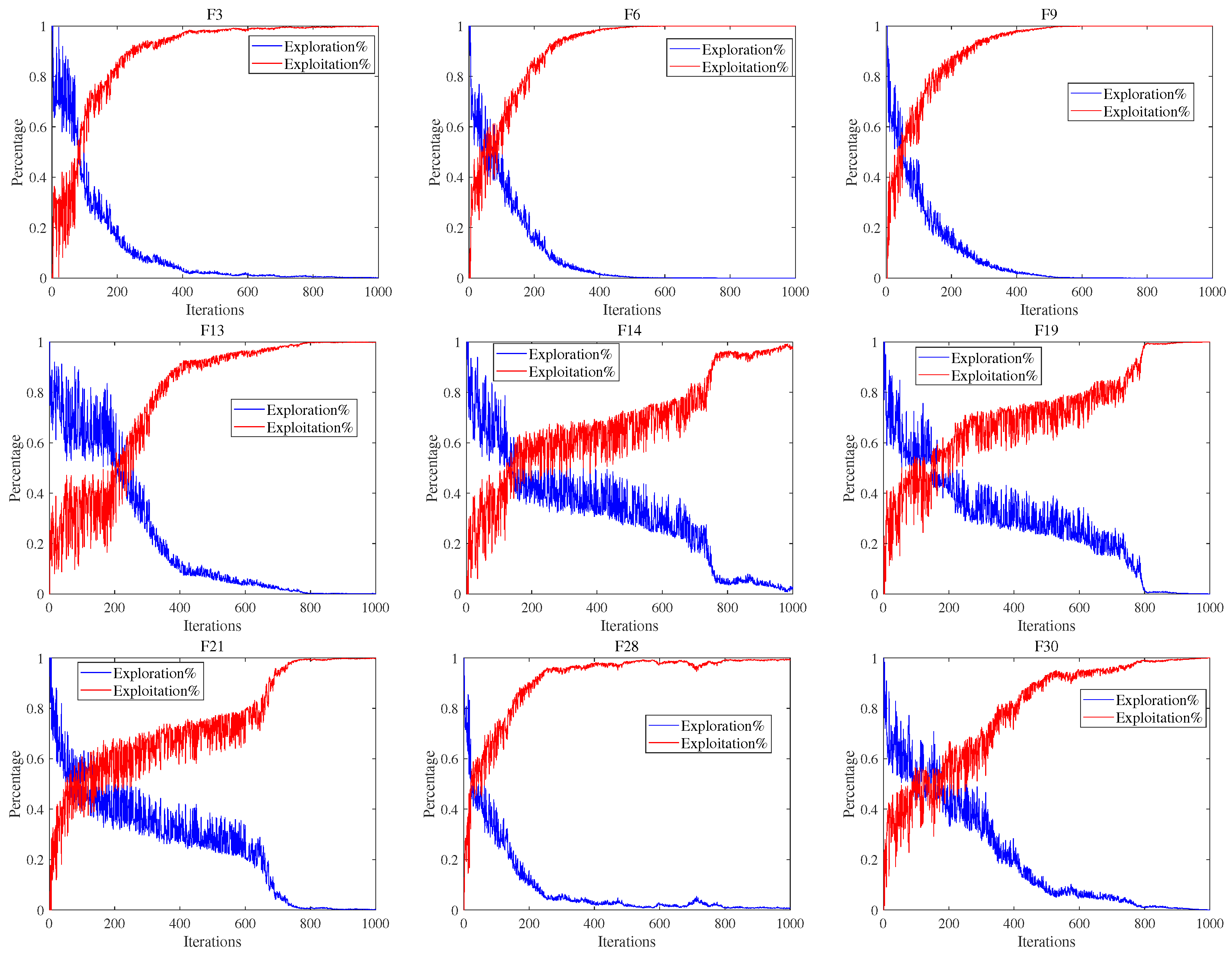
5.1.3. Exploration–Exploitation Analysis
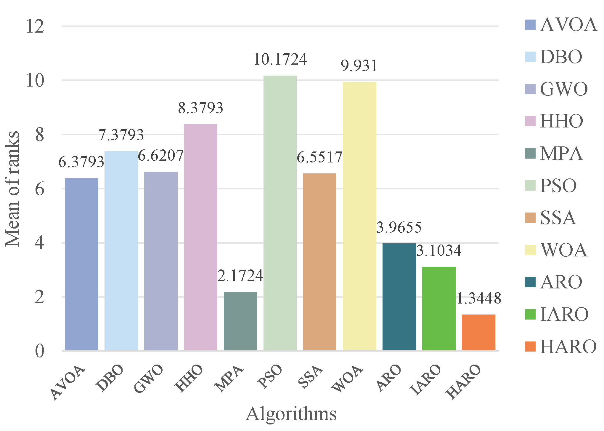
5.1.4. Non-Parametric Statistical Analysis
5.1.5. Ablation Study
5.2. Application of HARO+ in UAV Path Planning
5.2.1. Setting the Simulation Environment
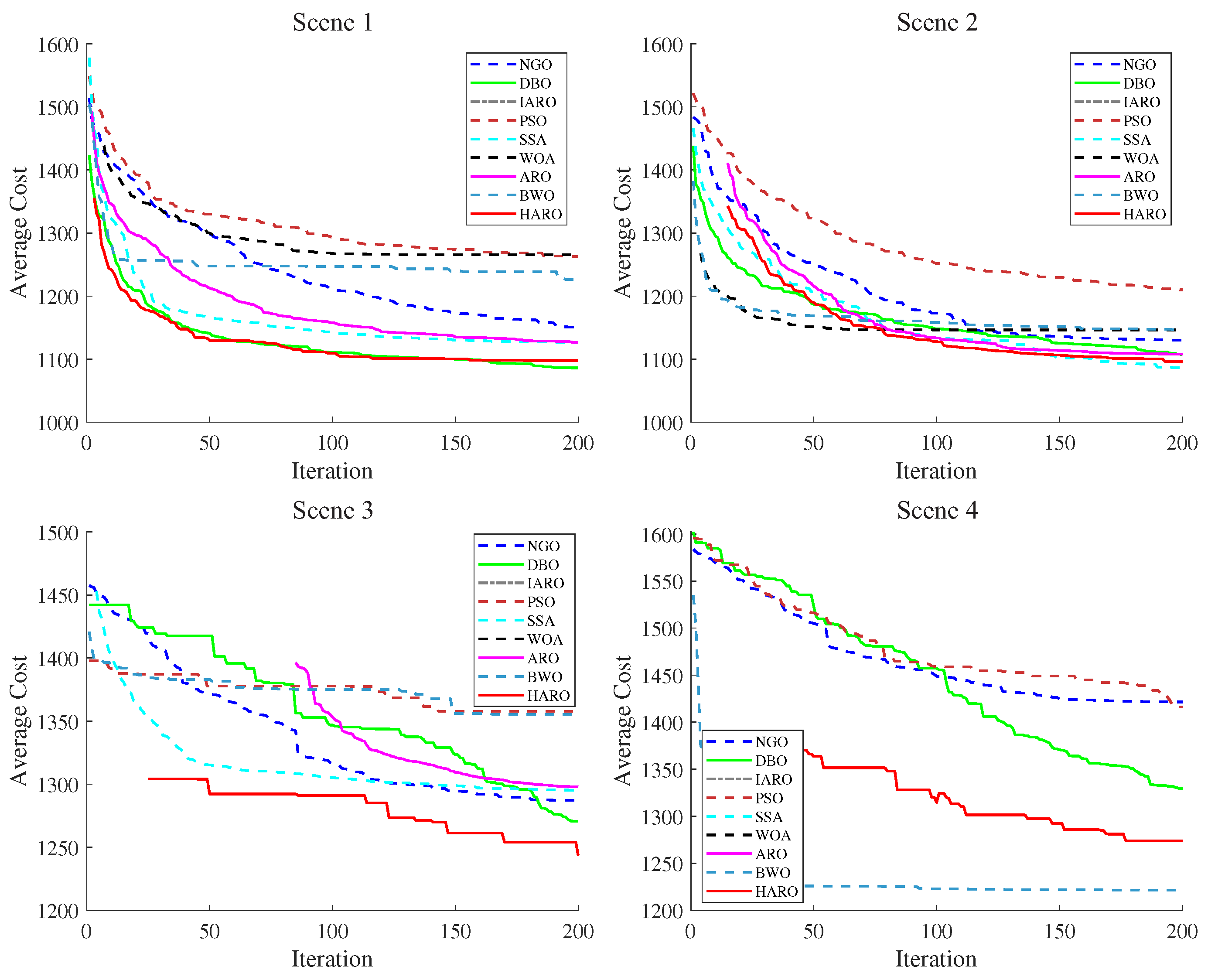
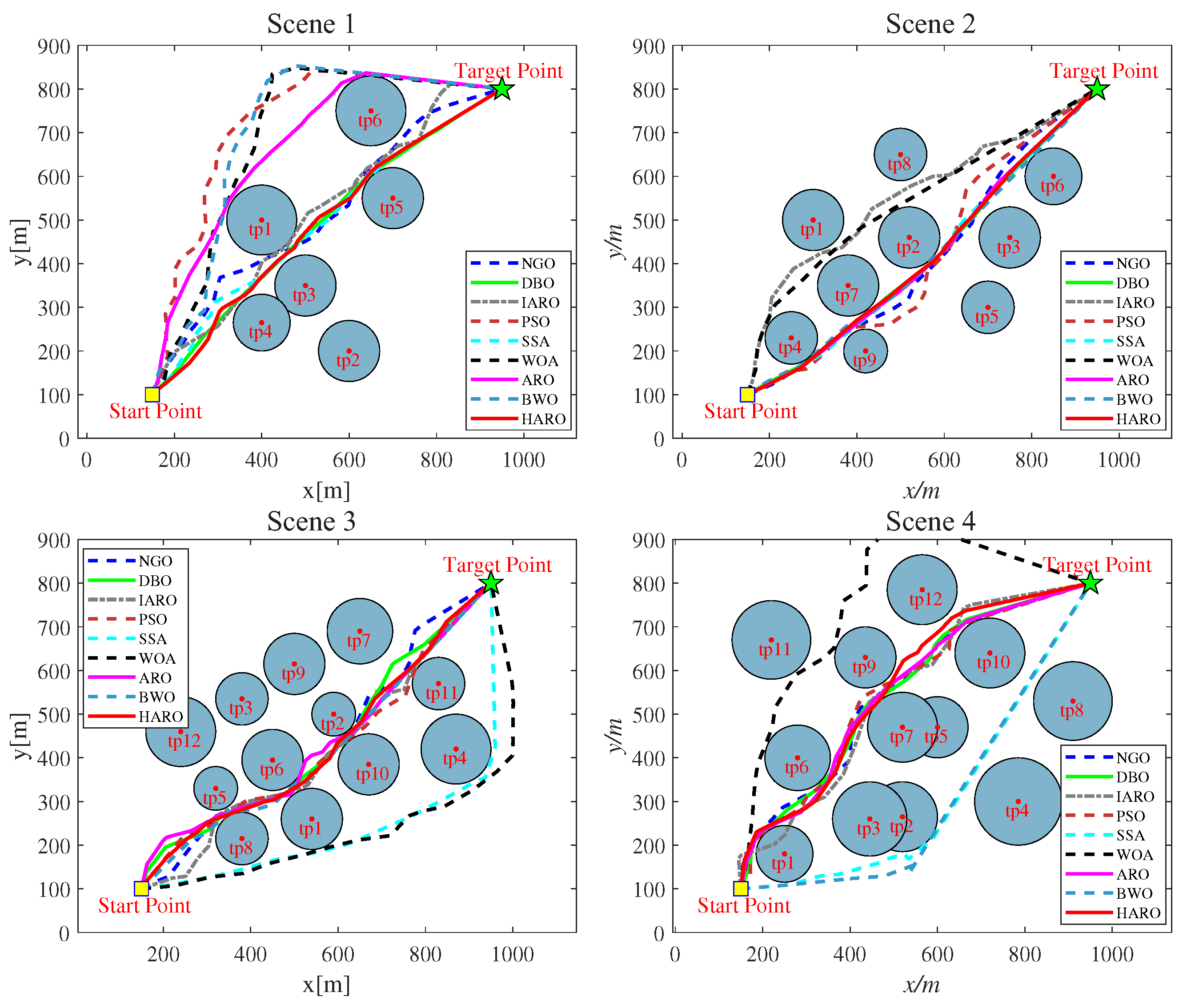
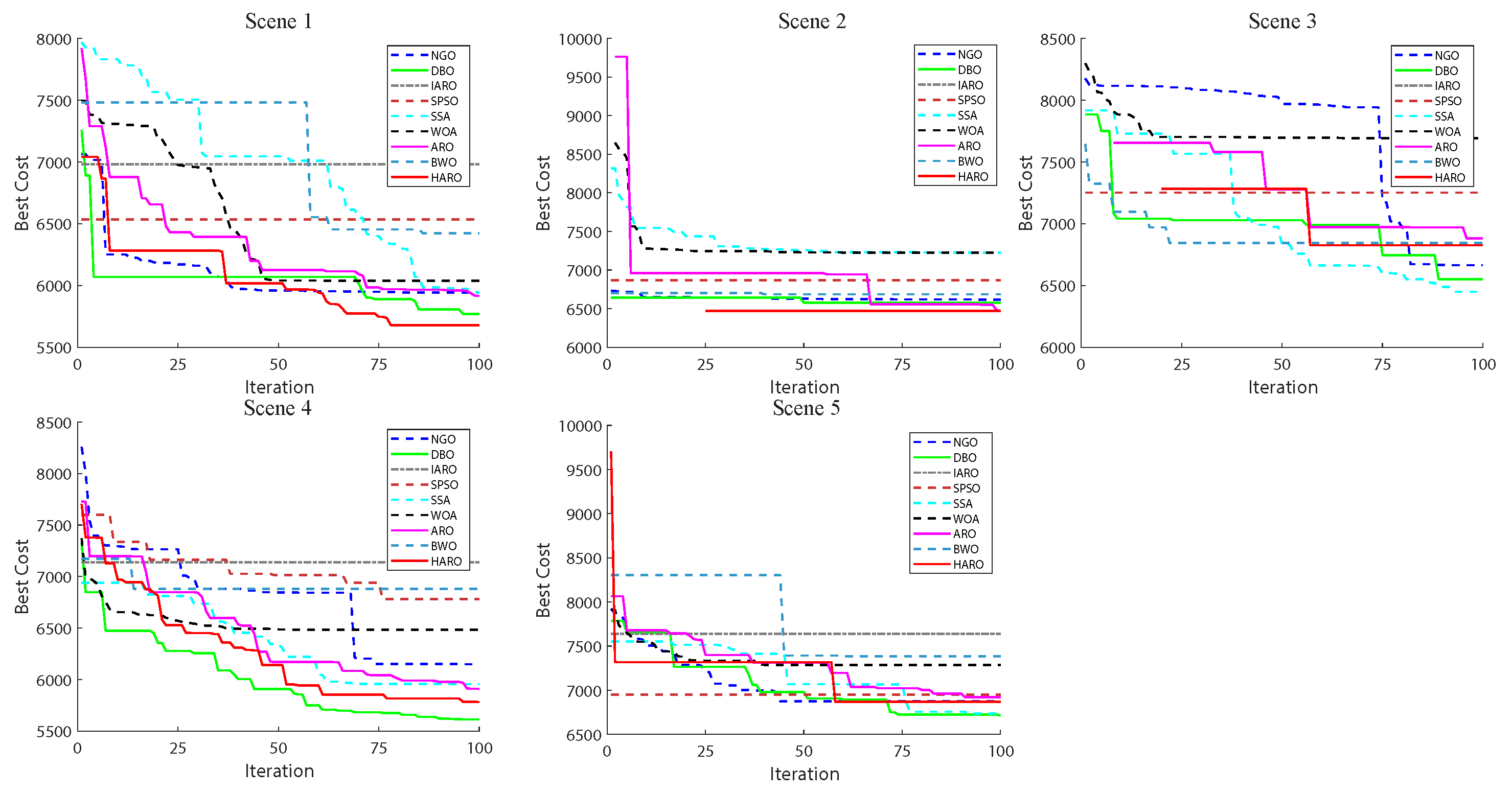
5.2.2. HARO for 2D UAV Path Planning
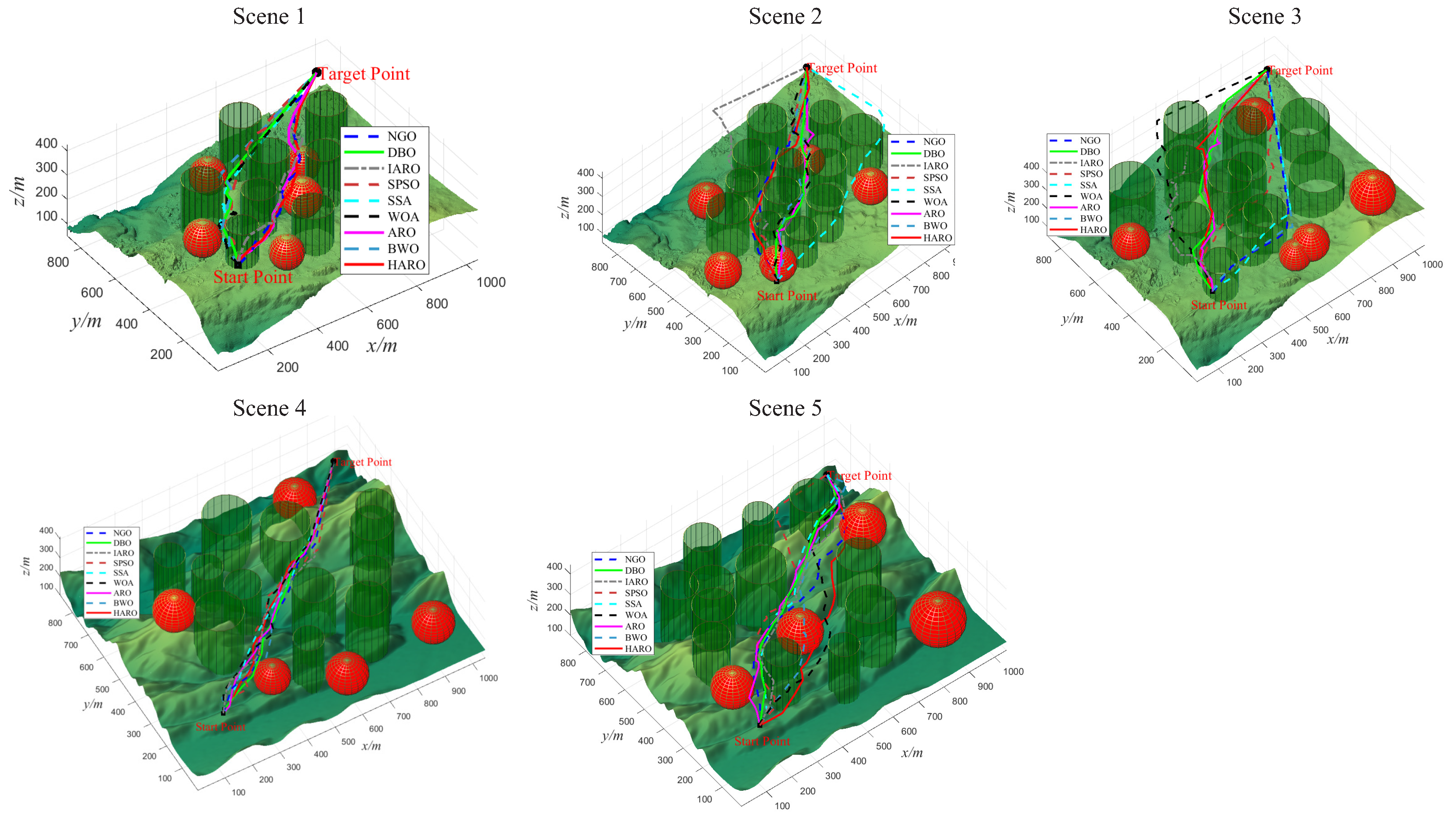
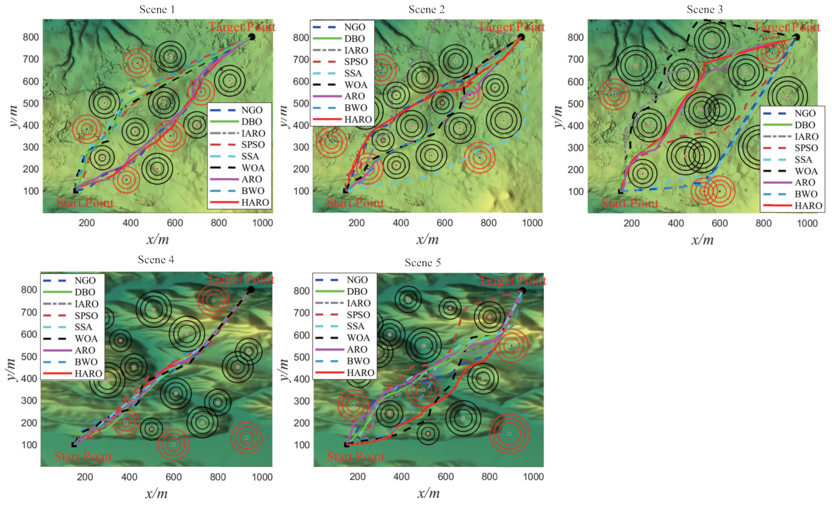
5.2.3. HARO for 3D UAV Path Planning
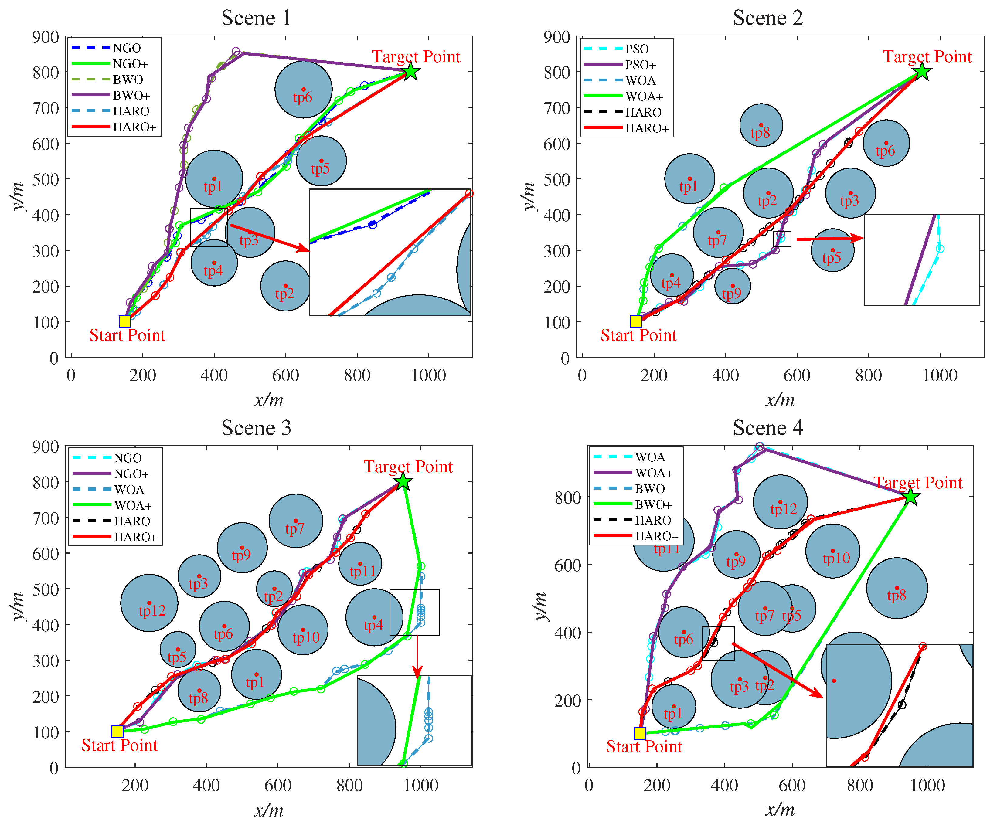
5.2.4. HARO+ with Trajectory Optimization in 2D/3D
6. Conclusions and Future Work
Author Contributions
Funding
Institutional Review Board Statement
Informed Consent Statement
Data Availability Statement
Conflicts of Interest
References
- Roberge, V.; Tarbouchi, M.; Labonté, G. Fast Genetic Algorithm Path Planner for Fixed-Wing Military UAV Using GPU. IEEE Trans. Aerosp. Electron. Syst. 2018, 54, 2105–2117. [Google Scholar] [CrossRef]
- Zhao, R.; Wang, Y.; Xiao, G.; Liu, C.; Hu, P.; Li, H. A method of path planning for unmanned aerial vehicle based on the hybrid of selfish herd optimizer and particle swarm optimizer. Appl. Intell. 2022, 52, 16775–16798. [Google Scholar] [CrossRef]
- Liu, X.; Li, G.; Yang, H.; Zhang, N.; Wang, L.; Shao, P. Agricultural UAV trajectory planning by incorporating multi-mechanism improved grey wolf optimization algorithm. Expert Syst. Appl. 2023, 233, 120946. [Google Scholar] [CrossRef]
- Liu, Y. An optimization-driven dynamic vehicle routing algorithm for on-demand meal delivery using drones. Comput. Oper. Res. 2019, 111, 1–20. [Google Scholar] [CrossRef]
- Huang, H.; Hu, C.; Zhu, J.; Wu, M.; Malekian, R. Stochastic Task Scheduling in UAV-Based Intelligent On-Demand Meal Delivery System. IEEE Trans. Intell. Transp. Syst. 2022, 23, 13040–13054. [Google Scholar] [CrossRef]
- Bakirci, M. Smart city air quality management through leveraging drones for precision monitoring. Sustain. Cities Soc. 2024, 106, 105390. [Google Scholar] [CrossRef]
- Tahir, A. Formation Control of Swarms of Unmanned Aerial Vehicles. Ph.D. Thesis, University of Turku, Turku, Finland, 2023. [Google Scholar]
- Shen, Q.; Zhang, D.; Xie, M.; He, Q. Multi-Strategy Enhanced Dung Beetle Optimizer and Its Application in Three-Dimensional UAV Path Planning. Symmetry 2023, 15, 1432. [Google Scholar] [CrossRef]
- Sun, C.; Tang, J.; Zhang, X. FT-MSTC*: An Efficient Fault Tolerance Algorithm for Multi-robot Coverage Path Planning. In Proceedings of the 2021 IEEE International Conference on Real-time Computing and Robotics (RCAR), Xining, China, 15–19 July 2021; pp. 107–112. [Google Scholar] [CrossRef]
- Deng, Y.; Chen, Y.; Zhang, Y.; Mahadevan, S. Fuzzy Dijkstra algorithm for shortest path problem under uncertain environment. Appl. Soft Comput. 2012, 12, 1231–1237. [Google Scholar] [CrossRef]
- Cai, Y.; Xi, Q.; Xing, X.; Gui, H.; Liu, Q. Path planning for UAV tracking target based on improved A-star algorithm. In Proceedings of the 2019 1st International Conference on Industrial Artificial Intelligence (IAI), Shenyang, China, 23–27 July 2019; pp. 1–6. [Google Scholar]
- Li, W.; Wang, L.; Zou, A.; Cai, J.; He, H.; Tan, T. Path Planning for UAV Based on Improved PRM. Energies 2022, 15, 7267. [Google Scholar] [CrossRef]
- Kelner, J.M.; Burzynski, W.; Stecz, W. Modeling UAV swarm flight trajectories using Rapidly-exploring Random Tree algorithm. J. King Saud-Univ.-Comput. Inf. Sci. 2024, 36, 101909. [Google Scholar] [CrossRef]
- Qu, C.; Gai, W.; Zhong, M.; Zhang, J. A novel reinforcement learning based grey wolf optimizer algorithm for unmanned aerial vehicles (UAVs) path planning. Appl. Soft Comput. 2020, 89, 106099. [Google Scholar] [CrossRef]
- Su, Y.; Dai, Y.; Liu, Y. A hybrid hyper-heuristic whale optimization algorithm for reusable launch vehicle reentry trajectory optimization. Aerosp. Sci. Technol. 2021, 119, 107200. [Google Scholar] [CrossRef]
- Chakraborty, S.; Sharma, S.; Saha, A.K.; Saha, A. A novel improved whale optimization algorithm to solve numerical optimization and real-world applications. Artif. Intell. Rev. 2022, 55, 1–112. [Google Scholar] [CrossRef]
- Mohapatra, P.; Nath Das, K.; Roy, S. A modified competitive swarm optimizer for large scale optimization problems. Appl. Soft Comput. 2017, 59, 340–362. [Google Scholar] [CrossRef]
- Nadimi-Shahraki, M.H.; Zamani, H.; Mirjalili, S. Enhanced whale optimization algorithm for medical feature selection: A COVID-19 case study. Comput. Biol. Med. 2022, 148, 105858. [Google Scholar] [CrossRef]
- Zhu, F.; Li, G.; Tang, H.; Li, Y.; Lv, X.; Wang, X. Dung beetle optimization algorithm based on quantum computing and multi-strategy fusion for solving engineering problems. Expert Systems with Applications 2024, 236, 121219. [Google Scholar] [CrossRef]
- Holland, J.H. Genetic Algorithms. Sci. Am. 1992, 267, 66–73. [Google Scholar] [CrossRef]
- Li, M.; Xu, G.; Zeng, L.; Lai, Q. Hybrid whale optimization algorithm based on symbiosis strategy for global optimization. Appl. Intell. 2023, 53, 16663–16705. [Google Scholar] [CrossRef]
- Li, M.; Xu, G.; Fu, Y.; Zhang, T.; Du, L. Improved whale optimization algorithm based on variable spiral position update strategy and adaptive inertia weight. J. Intell. Fuzzy Syst. 2022, 42, 1501–1517. [Google Scholar] [CrossRef]
- Storn, R.; Price, K. Differential evolution–a simple and efficient heuristic for global optimization over continuous spaces. J. Glob. Optim. 1997, 11, 341–359. [Google Scholar] [CrossRef]
- Kennedy, J.; Eberhart, R. Particle swarm optimization. In Proceedings of the ICNN’95—International Conference on Neural Networks, Perth, WA, Australia, 27 November 27–1 December 1995; Volume 4, pp. 1942–1948. [Google Scholar]
- Dorigo, M.; Birattari, M.; Stutzle, T. Ant colony optimization. IEEE Comput. Intell. Mag. 2006, 1, 28–39. [Google Scholar] [CrossRef]
- Yu, X.; Li, C.; Zhou, J. A constrained differential evolution algorithm to solve UAV path planning in disaster scenarios. Knowl.-Based Syst. 2020, 204, 106209. [Google Scholar] [CrossRef]
- Pehlivanoglu, Y.V.; Pehlivanoglu, P. An enhanced genetic algorithm for path planning of autonomous UAV in target coverage problems. Appl. Soft Comput. 2021, 112, 107796. [Google Scholar] [CrossRef]
- Phung, M.D.; Ha, Q.P. Motion-encoded particle swarm optimization for moving target search using UAVs. Appl. Soft Comput. 2020, 97, 106705. [Google Scholar] [CrossRef]
- Xu, X.; Xie, C.; Luo, Z.; Zhang, C.; Zhang, T. A multi-objective evolutionary algorithm based on dimension exploration and discrepancy evolution for UAV path planning problem. Inf. Sci. 2024, 657, 119977. [Google Scholar] [CrossRef]
- Phung, M.D.; Ha, Q.P. Safety-enhanced UAV path planning with spherical vector-based particle swarm optimization. Appl. Soft Comput. 2021, 107, 107376. [Google Scholar] [CrossRef]
- Wang, L.; Cao, Q.; Zhang, Z.; Mirjalili, S.; Zhao, W. Artificial rabbits optimization: A new bio-inspired meta-heuristic algorithm for solving engineering optimization problems. Eng. Appl. Artif. Intell. 2022, 114, 105082. [Google Scholar] [CrossRef]
- Alsaiari, A.O.; Moustafa, E.B.; Alhumade, H.; Abulkhair, H.; Elsheikh, A. A coupled artificial neural network with artificial rabbits optimizer for predicting water productivity of different designs of solar stills. Adv. Eng. Softw. 2023, 175, 103315. [Google Scholar] [CrossRef]
- Gülmez, B. Stock price prediction with optimized deep LSTM network with artificial rabbits optimization algorithm. Expert Syst. Appl. 2023, 227, 120346. [Google Scholar] [CrossRef]
- Yang, B.; Li, Y.; Huang, J.; Li, M.; Zheng, R.; Duan, J.; Fan, T.; Zou, H.; Liu, T.; Wang, J.; et al. Modular reconfiguration of hybrid PV-TEG systems via artificial rabbit algorithm: Modelling, design and HIL validation. Appl. Energy 2023, 351, 121868. [Google Scholar] [CrossRef]
- Dangi, D.; Telang Chandel, S.; Kumar Dixit, D.; Sharma, S.; Bhagat, A. An efficient model for sentiment analysis using artificial rabbits optimized vector functional link network. Expert Syst. Appl. 2023, 225, 119849. [Google Scholar] [CrossRef]
- Cao, Q.; Wang, L.; Zhao, W.; Yuan, Z.; Liu, A.; Gao, Y.; Ye, R. Vibration State Identification of Hydraulic Units Based on Improved Artificial Rabbits Optimization Algorithm. Biomimetics 2023, 8, 243. [Google Scholar] [CrossRef] [PubMed]
- Zhang, C.; Zhou, W.; Qin, W.; Tang, W. A novel UAV path planning approach: Heuristic crossing search and rescue optimization algorithm. Expert Syst. Appl. 2023, 215, 119243. [Google Scholar] [CrossRef]
- Yang, C.; Liu, Y.; Jiang, X.; Zhang, Z.; Wei, L.; Lai, T.; Chen, R. Non-Rigid Point Set Registration via Adaptive Weighted Objective Function. IEEE Access 2018, 6, 75947–75960. [Google Scholar] [CrossRef]
- Tahir, A.; Haghbayan, H.; Böling, J.M.; Plosila, J. Energy-Efficient Post-Failure Reconfiguration of Swarms of Unmanned Aerial Vehicles. IEEE Access 2023, 11, 24768–24779. [Google Scholar] [CrossRef]
- Zhao, L.; Shi, G. A method for simplifying ship trajectory based on improved Douglas–Peucker algorithm. Ocean Eng. 2018, 166, 37–46. [Google Scholar] [CrossRef]
- Faramarzi, A.; Heidarinejad, M.; Mirjalili, S.; Gandomi, A.H. Marine Predators Algorithm: A nature-inspired metaheuristic. Expert Syst. Appl. 2020, 152, 113377. [Google Scholar] [CrossRef]
- Huang, C.; Zhou, X.; Ran, X.; Wang, J.; Chen, H.; Deng, W. Adaptive cylinder vector particle swarm optimization with differential evolution for UAV path planning. Eng. Appl. Artif. Intell. 2023, 121, 105942. [Google Scholar] [CrossRef]
- Wang, W.; Ye, C.; Tian, J. SGGTSO: A Spherical Vector-Based Optimization Algorithm for 3D UAV Path Planning. Drones 2023, 7, 452. [Google Scholar] [CrossRef]
- Pan, Z.; Zhang, C.; Xia, Y.; Xiong, H.; Shao, X. An Improved Artificial Potential Field Method for Path Planning and Formation Control of the Multi-UAV Systems. IEEE Trans. Circuits Syst. II Express Briefs 2022, 69, 1129–1133. [Google Scholar] [CrossRef]
- Lin, K.; Li, Y.; Chen, S.; Li, D.; Wu, X. Motion Planner with Fixed-Horizon Constrained Reinforcement Learning for Complex Autonomous Driving Scenarios. IEEE Trans. Intell. Veh. 2024, 9, 1577–1588. [Google Scholar] [CrossRef]
- Lin, K.; Li, D.; Li, Y.; Chen, S.; Wu, X. FHCPL: An Intelligent Fixed-Horizon Constrained Policy Learning System for Risk-Sensitive Industrial Scenario. IEEE Trans. Ind. Inform. 2024, 20, 5794–5804. [Google Scholar] [CrossRef]
- Bai, X.; Xie, Z.; Xu, X.; Xiao, Y. An adaptive threshold fast DBSCAN algorithm with preserved trajectory feature points for vessel trajectory clustering. Ocean Eng. 2023, 280, 114930. [Google Scholar] [CrossRef]
- Tang, C.; Wang, H.; Zhao, J.; Tang, Y.; Yan, H.; Xiao, Y. A method for compressing AIS trajectory data based on the adaptive-threshold Douglas-Peucker algorithm. Ocean Eng. 2021, 232, 109041. [Google Scholar] [CrossRef]
- Awadallah, M.A.; Braik, M.S.; Al-Betar, M.A.; Abu Doush, I. An enhanced binary artificial rabbits optimization for feature selection in medical diagnosis. Neural Comput. Appl. 2023, 35, 20013–20068. [Google Scholar] [CrossRef]
- Luo, X.; Zou, H.; Hu, Y.; Gui, P.; Xu, Y.; Zhang, D.; Hu, W.; Hu, M. Synergistic registration of CT-MRI brain images and retinal images: A novel approach leveraging reinforcement learning and modified artificial rabbit optimization. Neurocomputing 2024, 585, 127506. [Google Scholar] [CrossRef]
- Hu, G.; Jing, W.; Houssein, E.H. Elite-based feedback boosted artificial rabbits-inspired optimizer with mutation and adaptive group: A case study of degree reduction for ball NURBS curves. Soft Comput. 2023, 27, 16919–16957. [Google Scholar] [CrossRef]
- Jiang, Y.; Wu, Q.; Zhu, S.; Zhang, L. Orca predation algorithm: A novel bio-inspired algorithm for global optimization problems. Expert Syst. Appl. 2022, 188, 116026. [Google Scholar] [CrossRef]
- Braik, M.; Hammouri, A.; Atwan, J.; Al-Betar, M.A.; Awadallah, M.A. White Shark Optimizer: A novel bio-inspired meta-heuristic algorithm for global optimization problems. Knowl.-Based Syst. 2022, 243, 108457. [Google Scholar] [CrossRef]
- Hu, G.; Huang, F.; Seyyedabbasi, A.; Wei, G. Enhanced multi-strategy bottlenose dolphin optimizer for UAVs path planning. Appl. Math. Model. 2024, 130, 243–271. [Google Scholar] [CrossRef]
- Douglas, D.H.; Peucker, T.K. Algorithms for the reduction of the number of points required to represent a digitized line or its caricature. Cartogr. Int. J. Geogr. Inf. Geovisualization 1973, 10, 112–122. [Google Scholar] [CrossRef]
- Abdel-Basset, M.; Mohamed, R.; Abouhawwash, M. Crested Porcupine Optimizer: A new nature-inspired metaheuristic. Knowl.-Based Syst. 2024, 284, 111257. [Google Scholar] [CrossRef]
- Parouha, R.P.; Das, K.N. A memory based differential evolution algorithm for unconstrained optimization. Appl. Soft Comput. 2016, 38, 501–517. [Google Scholar] [CrossRef]
- Opara, K.; Arabas, J. Comparison of mutation strategies in Differential Evolution—A probabilistic perspective. Swarm Evol. Comput. 2018, 39, 53–69. [Google Scholar] [CrossRef]
- Wu, G.; Mallipeddi, R.; Suganthan, P. Problem Definitions and Evaluation Criteria for the CEC 2017 Competition and Special Session on Constrained Single Objective Real-Parameter Optimization; Technology Report; Nanyang Technological University: Singapore, 2016; pp. 1–18. [Google Scholar]
- Mirjalili, S.; Lewis, A. The Whale Optimization Algorithm. Adv. Eng. Softw. 2016, 95, 51–67. [Google Scholar] [CrossRef]
- Mirjalili, S.; Mirjalili, S.M.; Lewis, A. Grey Wolf Optimizer. Adv. Eng. Softw. 2014, 69, 46–61. [Google Scholar] [CrossRef]
- Abdollahzadeh, B.; Gharehchopogh, F.S.; Mirjalili, S. African vultures optimization algorithm: A new nature-inspired metaheuristic algorithm for global optimization problems. Comput. Ind. Eng. 2021, 158, 107408. [Google Scholar] [CrossRef]
- Xue, J.; Shen, B. A novel swarm intelligence optimization approach: Sparrow search algorithm. Syst. Sci. Control. Eng. 2020, 8, 22–34. [Google Scholar] [CrossRef]
- Xue, J.; Shen, B. Dung beetle optimizer: A new meta-heuristic algorithm for global optimization. J. Supercomput. 2023, 79, 7305–7336. [Google Scholar] [CrossRef]
- Heidari, A.A.; Mirjalili, S.; Faris, H.; Aljarah, I.; Mafarja, M.; Chen, H. Harris hawks optimization: Algorithm and applications. Future Gener. Comput. Syst. 2019, 97, 849–872. [Google Scholar] [CrossRef]
- Morales-Castañeda, B.; Zaldívar, D.; Cuevas, E.; Fausto, F.; Rodríguez, A. A better balance in metaheuristic algorithms: Does it exist? Swarm Evol. Comput. 2020, 54, 100671. [Google Scholar] [CrossRef]
- Derrac, J.; García, S.; Molina, D.; Herrera, F. A practical tutorial on the use of nonparametric statistical tests as a methodology for comparing evolutionary and swarm intelligence algorithms. Swarm Evol. Comput. 2011, 1, 3–18. [Google Scholar] [CrossRef]
- Demšar, J. Statistical comparisons of classifiers over multiple data sets. J. Mach. Learn. Res. 2006, 7, 1–30. [Google Scholar]
- Dehghani, M.; Hubálovskỳ, Š.; Trojovskỳ, P. Northern goshawk optimization: A new swarm-based algorithm for solving optimization problems. IEEE Access 2021, 9, 162059–162080. [Google Scholar] [CrossRef]
- Zhong, C.; Li, G.; Meng, Z. Beluga whale optimization: A novel nature-inspired metaheuristic algorithm. Knowl.-Based Syst. 2022, 251, 109215. [Google Scholar] [CrossRef]
- Australia, G. Digital Elevation Model (DEM) of Australia Derived from LiDAR 5 Metre Grid; Commonwealth of Australia and Geoscience Australia: Canberra, Australia, 2015. [Google Scholar]
- Wolpert, D.; Macready, W. No free lunch theorems for optimization. IEEE Trans. Evol. Comput. 1997, 1, 67–82. [Google Scholar] [CrossRef]


| Fi | Index | AVOA | DBO | GWO | HHO | MPA | PSO | SSA | WOA | ARO | IARO | HARO |
|---|---|---|---|---|---|---|---|---|---|---|---|---|
| F1 | Mean | |||||||||||
| Std | ||||||||||||
| Best | ||||||||||||
| Rank | 5 | 7 | 10 | 8 | 6 | 11 | 3 | 9 | 4 | 1 | 2 | |
| F3 | Mean | |||||||||||
| Std | ||||||||||||
| Best | ||||||||||||
| Rank | 4 | 10 | 8 | 5 | 3 | 9 | 7 | 11 | 6 | 1 | 2 | |
| F4 | Mean | |||||||||||
| Std | ||||||||||||
| Best | ||||||||||||
| Rank | 6 | 7 | 9 | 8 | 3 | 11 | 4 | 10 | 5 | 1 | 2 | |
| F5 | Mean | |||||||||||
| Std | ||||||||||||
| Best | ||||||||||||
| Rank | 7 | 6 | 5 | 8 | 2 | 11 | 9 | 10 | 3 | 4 | 1 | |
| F6 | Mean | |||||||||||
| Std | ||||||||||||
| Best | ||||||||||||
| Rank | 7 | 6 | 5 | 9 | 4 | 11 | 8 | 10 | 2 | 3 | 1 | |
| F7 | Mean | |||||||||||
| Std | ||||||||||||
| Best | ||||||||||||
| Rank | 7 | 6 | 5 | 8 | 2 | 11 | 9 | 10 | 3 | 4 | 1 | |
| F8 | Mean | |||||||||||
| Std | ||||||||||||
| Best | ||||||||||||
| Rank | 6 | 9 | 4 | 7 | 2 | 11 | 8 | 10 | 5 | 3 | 1 | |
| F9 | Mean | |||||||||||
| Std | ||||||||||||
| Best | ||||||||||||
| Rank | 6 | 8 | 5 | 9 | 2 | 10 | 7 | 11 | 3 | 4 | 1 | |
| F10 | Mean | |||||||||||
| Std | ||||||||||||
| Best | ||||||||||||
| Rank | 6 | 7 | 4 | 9 | 2 | 11 | 8 | 10 | 5 | 3 | 1 | |
| F11 | Mean | |||||||||||
| Std | ||||||||||||
| Best | ||||||||||||
| Rank | 5 | 9 | 8 | 7 | 2 | 11 | 6 | 10 | 3 | 4 | 1 | |
| F12 | Mean | |||||||||||
| Std | ||||||||||||
| Best | ||||||||||||
| Rank | 6 | 8 | 9 | 7 | 2 | 11 | 5 | 10 | 4 | 3 | 1 | |
| F13 | Mean | |||||||||||
| Std | ||||||||||||
| Best | ||||||||||||
| Rank | 6 | 9 | 10 | 8 | 2 | 11 | 5 | 7 | 4 | 3 | 1 | |
| F14 | Mean | |||||||||||
| Std | ||||||||||||
| Best | ||||||||||||
| Rank | 7 | 8 | 10 | 9 | 2 | 5 | 6 | 11 | 4 | 3 | 1 | |
| F15 | Mean | |||||||||||
| Std | ||||||||||||
| Best | ||||||||||||
| Rank | 7 | 9 | 11 | 8 | 2 | 6 | 5 | 10 | 4 | 3 | 1 | |
| F16 | Mean | |||||||||||
| Std | ||||||||||||
| Best | ||||||||||||
| Rank | 6 | 7 | 4 | 9 | 1 | 11 | 8 | 10 | 5 | 3 | 2 | |
| F17 | Mean | |||||||||||
| Std | ||||||||||||
| Best | ||||||||||||
| Rank | 8 | 6 | 4 | 10 | 2 | 11 | 7 | 9 | 5 | 3 | 1 | |
| F18 | Mean | |||||||||||
| Std | ||||||||||||
| Best | ||||||||||||
| Rank | 8 | 10 | 7 | 9 | 2 | 5 | 6 | 11 | 4 | 3 | 1 | |
| F19 | Mean | |||||||||||
| Std | ||||||||||||
| Best | ||||||||||||
| Rank | 6 | 8 | 10 | 9 | 2 | 7 | 5 | 11 | 4 | 3 | 1 | |
| F20 | Mean | |||||||||||
| Std | ||||||||||||
| Best | ||||||||||||
| Rank | 7 | 6 | 5 | 9 | 2 | 11 | 8 | 10 | 4 | 3 | 1 | |
| F21 | Mean | |||||||||||
| Std | ||||||||||||
| Best | ||||||||||||
| Rank | 6 | 7 | 5 | 9 | 1 | 11 | 8 | 10 | 4 | 3 | 2 | |
| F22 | Mean | |||||||||||
| Std | ||||||||||||
| Best | ||||||||||||
| Rank | 6 | 8 | 5 | 9 | 4 | 11 | 7 | 10 | 2 | 3 | 1 | |
| F23 | Mean | |||||||||||
| Std | ||||||||||||
| Best | ||||||||||||
| Rank | 8 | 6 | 5 | 10 | 1 | 11 | 7 | 9 | 3 | 4 | 2 | |
| F24 | Mean | |||||||||||
| Std | ||||||||||||
| Best | ||||||||||||
| Rank | 8 | 6 | 4 | 10 | 2 | 11 | 7 | 9 | 3 | 5 | 1 | |
| F25 | Mean | |||||||||||
| Std | ||||||||||||
| Best | ||||||||||||
| Rank | 5 | 8 | 9 | 7 | 1 | 11 | 4 | 10 | 6 | 3 | 2 | |
| F26 | Mean | |||||||||||
| Std | ||||||||||||
| Best | ||||||||||||
| Rank | 7 | 6 | 4 | 9 | 1 | 11 | 8 | 10 | 3 | 5 | 2 | |
| F27 | Mean | |||||||||||
| Std | ||||||||||||
| Best | ||||||||||||
| Rank | 7 | 6 | 4 | 9 | 1 | 11 | 8 | 10 | 3 | 5 | 2 | |
| F28 | Mean | |||||||||||
| Std | ||||||||||||
| Best | ||||||||||||
| Rank | 5 | 8 | 9 | 7 | 3 | 11 | 4 | 10 | 6 | 1 | 2 | |
| F29 | Mean | |||||||||||
| Std | ||||||||||||
| Best | ||||||||||||
| Rank | 7 | 6 | 5 | 9 | 2 | 11 | 8 | 10 | 4 | 3 | 1 | |
| F30 | Mean | |||||||||||
| Std | ||||||||||||
| Best | ||||||||||||
| Rank | 6 | 7 | 9 | 8 | 2 | 11 | 5 | 10 | 4 | 3 | 1 |
| Function | AVOA | DBO | GWO | HHO | A, M.P. | PSO | SSA | WOA | ARO | IARO |
|---|---|---|---|---|---|---|---|---|---|---|
| F1 | ||||||||||
| F3 | ||||||||||
| F4 | ||||||||||
| F5 | ||||||||||
| F6 | ||||||||||
| F7 | ||||||||||
| F8 | ||||||||||
| F9 | ||||||||||
| F10 | ||||||||||
| F11 | ||||||||||
| F12 | ||||||||||
| F13 | ||||||||||
| F14 | ||||||||||
| F15 | ||||||||||
| F16 | ||||||||||
| F17 | ||||||||||
| F18 | ||||||||||
| F19 | ||||||||||
| F20 | ||||||||||
| F21 | ||||||||||
| F22 | ||||||||||
| F23 | ||||||||||
| F24 | ||||||||||
| F25 | ||||||||||
| F26 | ||||||||||
| F27 | ||||||||||
| F28 | ||||||||||
| F29 | ||||||||||
| F30 |
| Function | Index | ARO | EARO | DEARO | MARO | Function | Index | ARO | EARO | DEARO | MARO |
|---|---|---|---|---|---|---|---|---|---|---|---|
| F1 | Mean | F17 | Mean | ||||||||
| Std | Std | ||||||||||
| Best | Best | ||||||||||
| Rank | 3 | 4 | 2 | 1 | Rank | 4 | 3 | 2 | 1 | ||
| F3 | Mean | F18 | Mean | ||||||||
| Std | Std | ||||||||||
| Best | Best | ||||||||||
| Rank | 4 | 2 | 3 | 1 | Rank | 4 | 3 | 2 | 1 | ||
| F4 | Mean | F19 | Mean | ||||||||
| Std | Std | ||||||||||
| Best | Best | ||||||||||
| Rank | 4 | 2 | 3 | 1 | Rank | 4 | 3 | 2 | 1 | ||
| F5 | Mean | F20 | Mean | ||||||||
| Std | Std | ||||||||||
| Best | Best | ||||||||||
| Rank | 3 | 4 | 2 | 1 | Rank | 4 | 3 | 1 | 2 | ||
| F6 | Mean | F21 | Mean | ||||||||
| Std | Std | ||||||||||
| Best | Best | ||||||||||
| Rank | 3 | 4 | 2 | 1 | Rank | 4 | 3 | 1 | 2 | ||
| F7 | Mean | F22 | Mean | ||||||||
| Std | Std | ||||||||||
| Best | Best | ||||||||||
| Rank | 3 | 4 | 1 | 2 | Rank | 4 | 3 | 2 | 1 | ||
| F8 | Mean | F23 | Mean | ||||||||
| Std | Std | ||||||||||
| Best | Best | ||||||||||
| Rank | 4 | 3 | 2 | 1 | Rank | 4 | 3 | 1 | 2 | ||
| F9 | Mean | F24 | Mean | ||||||||
| Std | Std | ||||||||||
| Best | Best | ||||||||||
| Rank | 3 | 4 | 2 | 1 | Rank | 3 | 4 | 2 | 1 | ||
| F10 | Mean | F25 | Mean | ||||||||
| Std | Std | ||||||||||
| Best | Best | ||||||||||
| Rank | 4 | 1 | 3 | 2 | Rank | 4 | 2 | 3 | 1 | ||
| F11 | Mean | F26 | Mean | ||||||||
| Std | Std | ||||||||||
| Best | Best | ||||||||||
| Rank | 3 | 2 | 4 | 1 | Rank | 4 | 3 | 1 | 2 | ||
| F12 | Mean | F27 | Mean | ||||||||
| Std | Std | ||||||||||
| Best | Best | ||||||||||
| Rank | 4 | 2 | 3 | 1 | Rank | 4 | 2 | 3 | 1 | ||
| F13 | Mean | F28 | Mean | ||||||||
| Std | Std | ||||||||||
| Best | Best | ||||||||||
| Rank | 4 | 3 | 2 | 1 | Rank | 4 | 2 | 3 | 1 | ||
| F14 | Mean | F29 | Mean | ||||||||
| Std | Std | ||||||||||
| Best | Best | ||||||||||
| Rank | 4 | 3 | 2 | 1 | Rank | 4 | 3 | 2 | 1 | ||
| F15 | Mean | F30 | Mean | ||||||||
| Std | Std | ||||||||||
| Best | Best | ||||||||||
| Rank | 4 | 3 | 2 | 1 | Rank | 2 | 3 | 4 | 1 | ||
| F16 | Mean | ||||||||||
| Std | |||||||||||
| Best | |||||||||||
| Rank | 4 | 3 | 1 | 2 |
| Scenario | Algorithms | Mean | Best | Std. | Rank | Scenario | Algorithms | Mean | Best | Std. | Rank |
|---|---|---|---|---|---|---|---|---|---|---|---|
| 1 | NGO | 5 | 2 | NGO | 3 | ||||||
| DBO | 1 | DBO | 2 | ||||||||
| IARO | Inf | - | 9 | IARO | Inf | - | 8 | ||||
| PSO | 7 | PSO | 7 | ||||||||
| SSA | 3 | SSA | 4 | ||||||||
| WOA | 8 | WOA | Inf | - | 9 | ||||||
| ARO | 4 | ARO | 5 | ||||||||
| BWO | 6 | BWO | 6 | ||||||||
| HARO | 2 | HARO | 1 | ||||||||
| 3 | NGO | 5 | 4 | NGO | 5 | ||||||
| DBO | 3 | DBO | 3 | ||||||||
| IARO | Inf | Inf | - | 9 | IARO | Inf | - | 9 | |||
| PSO | 4 | PSO | 8 | ||||||||
| SSA | Inf | - | 7 | SSA | 1 | ||||||
| WOA | Inf | - | 8 | WOA | 6 | ||||||
| ARO | Inf | - | 6 | ARO | 4 | ||||||
| BWO | 1 | BWO | 7 | ||||||||
| HARO | 2 | HARO | 2 |
| Scenario | Algorithms | Mean | Best | Std. | Rank | Scenario | Algorithms | Mean | Best | Std. | Rank |
|---|---|---|---|---|---|---|---|---|---|---|---|
| 1 | NGO | 4 | 2 | NGO | 4 | ||||||
| DBO | 2 | DBO | 3 | ||||||||
| IARO | Inf | - | 9 | IARO | Inf | Inf | - | 9 | |||
| SPSO | 6 | SPSO | 6 | ||||||||
| SSA | 5 | SSA | 7 | ||||||||
| WOA | Inf | - | 8 | WOA | 8 | ||||||
| ARO | 3 | ARO | 2 | ||||||||
| BWO | 7 | BWO | 5 | ||||||||
| HARO | 1 | HARO | 1 | ||||||||
| 3 | NGO | 4 | 4 | NGO | 4 | ||||||
| DBO | 2 | DBO | 3 | ||||||||
| IARO | Inf | Inf | - | 9 | IARO | Inf | - | 9 | |||
| SPSO | 5 | SPSO | 5 | ||||||||
| SSA | Inf | - | 6 | SSA | Inf | - | 7 | ||||
| WOA | Inf | - | 8 | WOA | Inf | - | 8 | ||||
| ARO | Inf | - | 7 | ARO | 2 | ||||||
| BWO | 1 | BWO | 6 | ||||||||
| HARO | 3 | HARO | 1 | ||||||||
| 5 | NGO | 5 | |||||||||
| DBO | 1 | ||||||||||
| IARO | 9 | ||||||||||
| SPSO | 6 | ||||||||||
| SSA | 4 | ||||||||||
| WOA | 7 | ||||||||||
| ARO | 3 | ||||||||||
| BWO | 8 | ||||||||||
| HARO | 2 |
| Scenario | Algorithms | Mean | Best | Std. | Algorithms | Mean | Best | Std. | Path Points | Improve | CR |
|---|---|---|---|---|---|---|---|---|---|---|---|
| 1 | NGO | NGO+ | 408 | 0.59% | 61.82% | ||||||
| DBO | DBO+ | 316 | 0.11% | 47.88% | |||||||
| ARO | ARO+ | 376 | 0.08% | 56.97% | |||||||
| BWO | BWO+ | 386 | 1.76% | 58.48% | |||||||
| HARO | HARO+ | 363 | 0.12% | 55.00% | |||||||
| 2 | DBO | DBO+ | 429 | 4.50% | 65.00% | ||||||
| PSO | PSO+ | 444 | 4.47% | 67.27% | |||||||
| ARO | ARO+ | 306 | 0.38% | 46.36% | |||||||
| BWO | BWO+ | 361 | 2.48% | 54.70% | |||||||
| HARO | HARO+ | 454 | 3.75% | 68.79% | |||||||
| 3 | NGO | NGO+ | 392 | 2.88% | 59.39% | ||||||
| DBO | DBO+ | 414 | 0.65% | 62.73% | |||||||
| PSO | PSO+ | 424 | 1.33% | 64.24% | |||||||
| BWO | BWO+ | 135 | 0.11% | 20.45% | |||||||
| HARO | HARO+ | 428 | 0.62% | 64.85% | |||||||
| 4 | DBO | DBO | 310 | 0.23% | 46.97% | ||||||
| SSA | SSA | 287 | 0.33% | 43.48% | |||||||
| BWO | BWO+ | 244 | 0.17% | 36.97% | |||||||
| HARO | HARO | 327 | 0.29% | 49.55% |
| Scenario | Algorithms | Mean | Best | Std. | Algorithms | Mean | Best | Std. | Path Points | Improve | CR |
|---|---|---|---|---|---|---|---|---|---|---|---|
| 1 | NGO | NGO+ | 436 | 0.63% | 66.06% | ||||||
| DBO | DBO+ | 332 | 0.65% | 50.30% | |||||||
| SPSO | SPSO+ | 504 | 0.46% | 76.36% | |||||||
| SSA | SSA+ | 444 | 0.58% | 67.27% | |||||||
| ARO | ARO+ | 418 | 0.69% | 63.33% | |||||||
| BWO | BWO+ | 465 | 1.18% | 70.45% | |||||||
| HARO | HARO+ | 368 | 0.75% | 55.76% | |||||||
| 2 | NGO | NGO+ | 544 | 0.87% | 82.42% | ||||||
| DBO | DBO+ | 552 | 0.37% | 83.64% | |||||||
| SPSO | SPSO+ | 547 | 0.59% | 82.88% | |||||||
| SSA | SSA+ | 392 | 0.27% | 59.39% | |||||||
| WOA | WOA+ | 414 | 0.11% | 62.73% | |||||||
| ARO | ARO+ | 387 | 0.38% | 58.64% | |||||||
| BWO | BWO+ | 514 | 1.23% | 77.88% | |||||||
| HARO | HARO+ | 551 | 0.92% | 83.48% | |||||||
| 3 | NGO | NGO+ | 558 | 0.89% | 84.55% | ||||||
| DBO | DBO+ | 532 | 0.81% | 80.61% | |||||||
| SPSO | SPSO+ | 564 | 0.56% | 85.45% | |||||||
| BWO | BWO+ | 269 | 0.22% | 40.76% | |||||||
| HARO | HARO+ | 543 | 0.79% | 82.27% | |||||||
| 4 | NGO | NGO+ | 506 | 0.42% | 76.67% | ||||||
| DBO | DBO+ | 505 | 0.83% | 76.52% | |||||||
| SPSO | SPSO+ | 519 | 0.38% | 78.64% | |||||||
| ARO | ARO+ | 518 | 0.58% | 78.48% | |||||||
| BWO | BWO+ | 546 | 0.71% | 82.73% | |||||||
| HARO | HARO+ | 502 | 1.21% | 76.06% | |||||||
| 5 | NGO | NGO+ | 437 | 0.91% | 66.21% | ||||||
| DBO | DBO+ | 378 | 0.46% | 57.27% | |||||||
| IARO | IARO+ | 503 | 1.44% | 76.21% | |||||||
| SPSO | SPSO+ | 504 | 0.60% | 76.36% | |||||||
| SSA | SSA+ | 421 | 0.56% | 63.79% | |||||||
| WOA | WOA+ | 498 | 0.72% | 75.45% | |||||||
| ARO | ARO+ | 374 | 0.23% | 56.67% | |||||||
| BWO | BWO+ | 484 | 1.71% | 73.33% | |||||||
| HARO | HARO+ | 406 | 0.23% | 61.52% |
Disclaimer/Publisher’s Note: The statements, opinions and data contained in all publications are solely those of the individual author(s) and contributor(s) and not of MDPI and/or the editor(s). MDPI and/or the editor(s) disclaim responsibility for any injury to people or property resulting from any ideas, methods, instructions or products referred to in the content. |
© 2024 by the authors. Licensee MDPI, Basel, Switzerland. This article is an open access article distributed under the terms and conditions of the Creative Commons Attribution (CC BY) license (https://creativecommons.org/licenses/by/4.0/).
Share and Cite
Liu, B.; Cai, Y.; Li, D.; Lin, K.; Xu, G. A Hybrid ARO Algorithm and Key Point Retention Strategy Trajectory Optimization for UAV Path Planning. Drones 2024, 8, 644. https://doi.org/10.3390/drones8110644
Liu B, Cai Y, Li D, Lin K, Xu G. A Hybrid ARO Algorithm and Key Point Retention Strategy Trajectory Optimization for UAV Path Planning. Drones. 2024; 8(11):644. https://doi.org/10.3390/drones8110644
Chicago/Turabian StyleLiu, Bei, Yuefeng Cai, Duantengchuan Li, Ke Lin, and Guanghui Xu. 2024. "A Hybrid ARO Algorithm and Key Point Retention Strategy Trajectory Optimization for UAV Path Planning" Drones 8, no. 11: 644. https://doi.org/10.3390/drones8110644
APA StyleLiu, B., Cai, Y., Li, D., Lin, K., & Xu, G. (2024). A Hybrid ARO Algorithm and Key Point Retention Strategy Trajectory Optimization for UAV Path Planning. Drones, 8(11), 644. https://doi.org/10.3390/drones8110644