Deep Reinforcement Learning-Based Wind Disturbance Rejection Control Strategy for UAV

Abstract

Unmanned aerial vehicles (UAVs) face significant challenges in maintaining stability when subjected to external wind disturbances and internal noise. This paper addresses these issues by introducing a real-time wind speed fitting algorithm and a wind field model that accounts for varying wind conditions, such as wind shear and turbulence. To improve control in such conditions, a deep reinforcement learning (DRL) strategy is developed and tested through both simulations and real-world experiments. The results indicate a 65% reduction in trajectory tracking error with the DRL controller. Additionally, a UAV built for testing exhibited enhanced stability and reduced angular deviations in wind conditions up to level 5. These findings demonstrate the effectiveness of the proposed DRL-based control strategy in increasing UAV resilience to wind disturbances.

1. Introduction

Quadcopters are widely used in civil, police, and military domains because of their versatility, stability, and cost-effective features [1]. In the civil domain, high-resolution digital imagery captured by drones is being used to detect coastal erosion processes [2]. In line inspection, unmanned aerial vehicle (UAV) clusters provide fast and accurate automated inspection solutions for distribution lines [3]. In the police domain, UAVs function as surveillance and tracking platforms for policing [4]. Additionally, UAVs function as aerial base stations in post-disaster communication recovery efforts to enhance wireless network coverage [5]. UAV technology continues to evolve, and the demand for UAVs in the military sector is growing rapidly, especially on the battlefield [6]. Intelligent planning and scheduling of battlefields through UAVs provides situational awareness of complex battlefields [7]. In surveillance and reconnaissance missions using UAVs, civilian and military personnel on the battlefield can be identified [8]. To tackle complex and changing mission environments, UAVs need to improve their flight stability and responsiveness to perturbations [9]. This necessity has led to the development of various control strategies aimed at improving UAV stability during flight and facilitating rapid recovery from disturbances. For attitude control of UAVs, a fuzzy PID controller to reduce instability and an adaptive flight controller based on dynamic inversion and linear neural networks have been proposed for precise attitude and trajectory control [10,11]. Additionally, flight control faces challenges in handling the underactuated, non-linear, and highly coupled system characteristics of the UAV dynamics model [12]. Neural networks have been employed to address such complexities through real-time learning of unknown system dynamics, achieving precise control despite model and parameter uncertainties [13]. Previous studies have employed two distinct control strategies to address control quality and perturbation resistance. These include a controller utilizing a self-resistant strategy and a robust controller integrating sliding mode control and inverse step control techniques, primarily aimed at ensuring system stability [14,15]. Taking into account practical application scenarios and research and development costs, PID control can be considered as an option to balance control performance and algorithm complexity [16]. Previous studies implemented a dual-loop PID controller for flight control and obstacle avoidance in UAVs, integrating both PID and self-resistant control methods [17,18].

However, during complex missions, UAVs often face challenges from wind disturbances, which can significantly affect their trajectory tracking and stabilization [19]. Wind disturbances can cause deviations from intended flight paths, leading to operational inefficiencies and potentially compromising mission success. Therefore, addressing these disturbances is critical for enhancing UAV reliability and performance in real-world applications [20]. Previous studies have introduced various control techniques, including disturbance observers and adaptive control strategies, to suppress external disturbances like wind in real time, improving UAV robustness in complex environments [21]. The maximum wind speed that a UAV can withstand in a wind field has been analyzed through the construction of a composite wind field model [22]. This insight informs the design of effective control strategies to enhance UAV performance in dynamic wind conditions. Additionally, an adaptive sliding mode controller has been designed to enhance the flight stability of UAVs in urban wind-disturbed environments [23]. While prior analyses have constructed composite wind field models to assess the maximum wind speeds that UAVs can withstand, many existing control systems primarily consider constant-value mean wind, neglecting the unpredictable, ever-changing winds that UAVs frequently encounter [19]. This gap highlights the necessity for improved control strategies that can adapt to real-world wind conditions, thereby enhancing UAV performance in dynamic environments. By effectively managing wind disturbances, UAVs can maintain stability and trajectory tracking, which is essential for successful missions in critical applications such as search and rescue, surveillance, and disaster response [24].

Furthermore, wind speed is not a purely random signal; it exhibits certain fractal characteristics with predictability over short periods [25]. Previous studies using fractal dimensions to study the long-term persistence of daily gust data have shown that the wind speed series exhibit fractal behaviour, and fractal multiple analysis and power spectral analysis of wind speed time series recorded at different meteorological stations have similarly shown the fractal behaviour of the wind speed time series and its low-dimensional chaotic nature [26,27].

The capability of DRL to solve decision-making problems in complex environments further supports our approach [28]. Developing agents based on data from visual obstacle information through DRL reduces time consumption while increasing efficiency [29]. Training a UAV to detect nearby obstacles using depth imagery and geo-fencing shows that the agent can successfully learn and avoid obstacles in the environment [30]. The effectiveness of the DRL feed-forward compensator was demonstrated using the DRL in a feed-forward compensating manner using the Lyapunov stability evidence determination [31]. Using historical state observations as input information to participate in UAV control is an advantage of deep reinforcement learning algorithms [32]. The UAV continuously learns the best action from the environment using historical reinforcement state observation data, which can effectively reduce the overall delay and the energy consumption of the UAV [33]. A DRL path planning method is proposed using the model of the UAV under constraints and the historical observation data of the threat zone, and the results show that the method is effective in obstacle avoidance and consumes less energy [34]. The effectiveness of the control effects of deep reinforcement learning is further demonstrated by real data-based trained agents performing real tests and validations [35].

Based on the literature review, it can be concluded that the challenge of ensuring UAV stability in varying wind conditions has garnered significant attention in recent research. The following section reviews notable works that focus on wind resistance and control strategies, particularly highlighting the application of DRL and other methodologies.

Several studies have tackled the issue of wind resistance in UAVs. For example, ref. [36] analyzes the wind resistance stability of multi-rotor UAVs, establishing a wind static model to evaluate performance under high-wind conditions. While this work offers valuable insights into structural design and safety, it primarily addresses static evaluations rather than dynamic control adaptations, which are critical in real-time applications. Similarly, ref. [19] emphasizes the importance of quantifying wind resistance by analyzing the induced velocity and thrust of multi-rotor UAVs. Although this research presents a method for measuring wind resistance, it lacks an integrated control approach, limiting its applicability to real-time scenarios where dynamic adjustments are necessary. In terms of control strategies, ref. [37] introduces an acceleration feedback-enhanced H-infinity controller designed to improve UAV performance against wind disturbances. While the H-infinity approach demonstrates robustness in trajectory tracking, its complexity may hinder practical implementation, particularly in rapidly changing wind environments where adaptability is essential. Another noteworthy contribution is made by [38], which proposes a distributed adaptive control strategy based on a leader–follower model. This method effectively counteracts lateral errors induced by wind disturbances. However, it does not address the complexities of various wind field models, limiting its generalizability.

The application of DRL in UAV control is particularly promising. In [39], a DRL agent is developed to enhance landing precision on dynamic platforms, demonstrating significant improvements in performance under wind-induced disturbances. While this study effectively showcases DRL’s capabilities, its focus is primarily on landing scenarios, not encompassing broader operational challenges. In urban contexts, ref. [40] explores the 3D path planning problem for UAVs affected by wind, utilizing a modified DRL algorithm. While it presents effective strategies for obstacle avoidance, further refinement in integrating wind dynamics could improve its real-world applicability. Additionally, ref. [41] tackles UAV navigation through a distributed DRL framework, which enhances convergence rates in high-dynamic environments. However, this study does not directly address wind disturbance compensation, which is critical for the reliability of UAV operations in unpredictable conditions. Moreover, ref. [42] introduces a DRL-based end-to-end control method for dynamic target tracking. This innovative approach simplifies traditional control paradigms but does not sufficiently consider the challenges posed by environmental factors, such as wind.

The literature highlights a gap in integrated approaches that combine robust wind disturbance handling with advanced control strategies. The research aims to fill this gap by integrating real-time wind speed fractal analysis with a DRL-based control strategy. This approach not only enhances UAV stability and adaptability under varying wind conditions but also addresses existing limitations by providing a comprehensive framework. By leveraging the strengths of both DRL and traditional control methods, the solution promises to improve operational efficiency, making it particularly relevant for applications in unpredictable environments.

This paper proposes a PID-DRL disturbance compensation controller for UAVs, utilizing a wind speed time series fractal feature dataset to enhance trajectory tracking performance. DRL has proven to be an effective method for solving complex decision-making problems, particularly in dynamic and uncertain environments, making it well suited for UAV control. Meanwhile, PID controllers are widely adopted due to their simplicity and reliability in maintaining stability and achieving desired performance across various applications. By integrating DRL with PID control, our strategy seeks to combine the strengths of both approaches to improve trajectory tracking under challenging wind conditions. The approach utilizes a wind speed time series fractal feature dataset to train the DRL compensator, enhancing its robustness in dynamic wind environments. Additionally, we introduce a segmented training method for the DRL model to reduce training time and increase overall efficiency. The key contributions of this study are summarized as follows:

• The integration of real-time wind speed fractal analysis with a DRL control strategy, enhancing the UAV’s ability to adapt to changing wind conditions.
• The establishment of a composite wind field model that incorporates the fractal characteristics of real wind speed time series, allowing for more accurate and responsive control.
• The development of a unique method for dynamically training the DRL controller using real-time wind speed data, improving the compensator’s effectiveness and robustness in trajectory tracking.

The remainder of the paper is organized as follows: Section 2 formulates the encountered problems and performs systematic modelling, Section 3 presents the main results of the study and analyzes them, and Section 4 concludes the study.

2. Problem Formulation and System Modelling

The PID-DRL control system is designed to train the agent within a composite wind field environment, enabling the UAV to effectively resist wind disturbances. Figure 1 illustrates the components and processes of the PID-DRL trajectory tracking control system. The training begins with the UAV operating in four typical wind fields, where it is tasked with hovering, cruising, or following a specified path. The UAV executes these tasks using predetermined controller and path parameters. Throughout this process, the UAV’s state is continuously updated based on environmental feedback, while actions are generated by the DRL algorithm. The reward function is critical, as it evaluates the deviation between the actual and desired paths. The training involves interactions with the environment to update the reward, with the ultimate goal of minimizing the state error between the UAV’s trajectory and the expected path.

The core challenge tackled in this study is how to effectively mitigate the destabilizing effects of wind disturbances on UAVs, particularly during trajectory tracking and hovering operations. Wind disturbances are a significant problem for UAVs, as they can cause deviations from intended flight paths and reduce control stability. The goal of this work is to develop a control framework that can maintain UAV stability and reduce tracking errors in the presence of unpredictable wind conditions. To achieve this, we propose a system framework, as illustrated in Figure 2, that integrates four main components: wind field perturbation, RL control, the control framework, and flight tests.

The wind field perturbation component models the real-time wind speed by utilizing fractal characteristics from measured wind data, creating a composite wind field in a simulated environment. This model is further validated using R/S analysis to calculate the Hurst exponent, ensuring the accuracy of the wind field’s representation. To combat the effects of these disturbances on UAV flight, we introduce an RL-based compensator. This compensator is designed to dynamically adjust control strategies based on the changing wind conditions. The RL training process is divided into multiple stages, each corresponding to specific flight tasks, and uses tailored reward functions to optimize control performance. The synergy between the wind field perturbation model and the RL compensator enables the UAV to maintain stability and accurately track its intended trajectory, in both simulations and real-world tests. The system’s robustness is evaluated under various wind conditions, with a focus on testing at a minimum wind level of 5.

2.1. System Modelling

According to [43], the air resistance due to wind speed perturbation is shown as follows:

$$F_w={\displaystyle \frac{\rho S{C}_w{u}_w^2}{2}}$$

(1)

where $\rho$ represents air density, S is the effective area of the fuselage, $C_w$ is the wind speed size component of the wind field, and $F_w$ denotes the air resistance acting on the directional component. According to the real site, wind speed exhibits uninterrupted and gradual changes. Therefore, the air resistance $F_w$ caused by the wind disturbance is continuous and microscopic.

Using the Newton–Euler equations as a basis, the following UAV dynamics model is developed to study the effects of trajectory tracking from take-off to a fixed-height cruise [44]. During take-off and rise, the UAV’s pitch angle changes dramatically due to wind shear [45]. The dynamic model not only represents the fundamental movements of the UAV but also incorporates wind disturbance factors, making it capable of reflecting the impact of wind speeds on both translational and rotational motion. By embedding wind disturbances into the dynamics, the model plays a critical role in simulating real-world environmental conditions and ensuring the UAV can handle varying wind forces.

Moreover, the dynamic model serves as the primary target for the control strategies designed later in the paper. The control strategies are applied to regulate the parameters within this model, enabling precise trajectory tracking and disturbance rejection, which is key to improving the UAV’s stability and performance under wind disturbances. Therefore, the dynamic model is crucial in linking the UAV’s physical behavior to the controller’s ability to achieve the desired trajectory in real-world conditions.

$$\left\{\begin{array}{c}\ddot{x}=(cos\psi sin\theta cos\varphi +sin\psi sin\varphi ){\displaystyle \frac{U_1}{m}}-{\displaystyle \frac{\rho S_x{C}_{Wx}{u}_W^2}{2m}}\hfill \\ \ddot{y}=(sin\psi sin\theta cos\varphi +sin\varphi cos\psi ){\displaystyle \frac{U_1}{m}}-{\displaystyle \frac{\rho S_y{C}_{Wy}{v}_W^2}{2m}}\hfill \\ \ddot{z}=cos\theta cos\varphi {\displaystyle \frac{U_1}{m}}-g-{\displaystyle \frac{\rho S_z{C}_{Wz}{w}_W^2}{2m}}\hfill \\ \dot{p}={\displaystyle \frac{L{U}_2+(I_{yy}-I_{zz})qr-J_{r}q\Omega -M_{Wx}}{I_{xx}}}\hfill \\ \dot{q}={\displaystyle \frac{L{U}_3+(I_{\mathrm{zz}}-I_{xx})pr+J_{r}q\Omega -M_{Wy}}{I_{yy}}}\hfill \\ \dot{r}={\displaystyle \frac{U_4+(I_{xx}-I_{yy})pq-M_{Wz}}{I_{zz}}}\hfill \\ \dot{\varphi }=p+(sin\varphi +rcos\varphi )tan\theta \hfill \\ \dot{\theta }=qcos\theta -rsin\varphi \hfill \\ \dot{\psi }=(qsin\varphi +rcos\varphi )/cos\theta \hfill \end{array}\right.$$

(2)

where the elements and the definitions involved in Equations (2) and (3) are shown in

Table 1. Table of variables.

Variable	Description
$\varphi$	Roll angle
$\theta$	Pitch angle
$\psi$	Yaw angle
x	UAV position in the inertial coordinate system
y	UAV position in the inertial coordinate system
z	UAV position in the inertial coordinate system
$u_W$	Wind speed component in the x direction
$v_W$	Wind speed component in the y direction
$w_W$	Wind speed component in the z direction
p	Angular velocity around the x axis
q	Angular velocity around the y axis
r	Angular velocity around the z axis
$S_x$	Effective area of the fuselage in the x direction
$S_y$	Effective area of the fuselage in the y direction
$S_z$	Effective area of the fuselage in the z direction
$U_1$	Total lift force generated by the UAV
$U_2$	Rotational moment along the body coordinate system
$U_3$	Rotational moment along the body coordinate system
$U_4$	Rotational moment along the body coordinate system
m	Mass of the UAV
g	Gravitational acceleration
L	Arm length of the UAV
$I_{xx}$	Rotational moment of inertia around x axis
$I_{yy}$	Rotational moment of inertia around y axis
$I_{zz}$	Rotational moment of inertia around z axis
$J_r$	Rotational moment of inertia of the motors
${\Omega }_i$	Rotational speed of the rotor blades
$\Omega$	Residual rotational speed of the wings
$M_W$	Aerodynamic drag moment under wind disturbance

.

$$\Omega ={\Omega }_1-{\Omega }_2+{\Omega }_3-{\Omega }_4$$

(3)

$M_W$ denotes the aerodynamic drag moment of the UAV under wind disturbance:

$$M_W=\sqrt{2}/2L{F}_w$$

(4)

2.2. Reinforcement Learning Trajectory Tracking Controller

In this paper, a dual-loop PID attitude controller is used to design a PID-DRL UAV anti-disturbance trajectory tracking controller, and the controller structure is shown in Figure 2 Control Flow. Among them, the final output of the position controller, the desired attitude angle ${\eta }_d$, is obtained by the summation of the control quantity ${\eta }_{PID}$ output from the PID controller and the compensated control quantity ${\eta }_{drl}$ output from the reinforcement learning compensator. The input of the PID controller is the difference $P_e$ between the desired position $P_d$ and the actual position $P_{x,y,z}$, and the input of the DRL controller has a total of 12 dimensions, which contains the UAV’s position error $P_e$, acceleration $\overrightarrow{a}$, UAV attitude $\eta$, and PID controller output ${\eta }_{PID}$.

The PID trajectory tracking control scheme is a classical dual-loop structure composed of an outer position loop and an inner attitude loop. The outer loop corrects the UAV’s position by minimizing the error between the desired trajectory and the current UAV position, while the inner loop stabilizes the UAV’s attitude based on position error feedback. The error-based control method enables precise adjustments to the UAV’s motion and attitude, allowing for reliable tracking of a given path. This ensures robust trajectory tracking, even under disturbances such as wind.

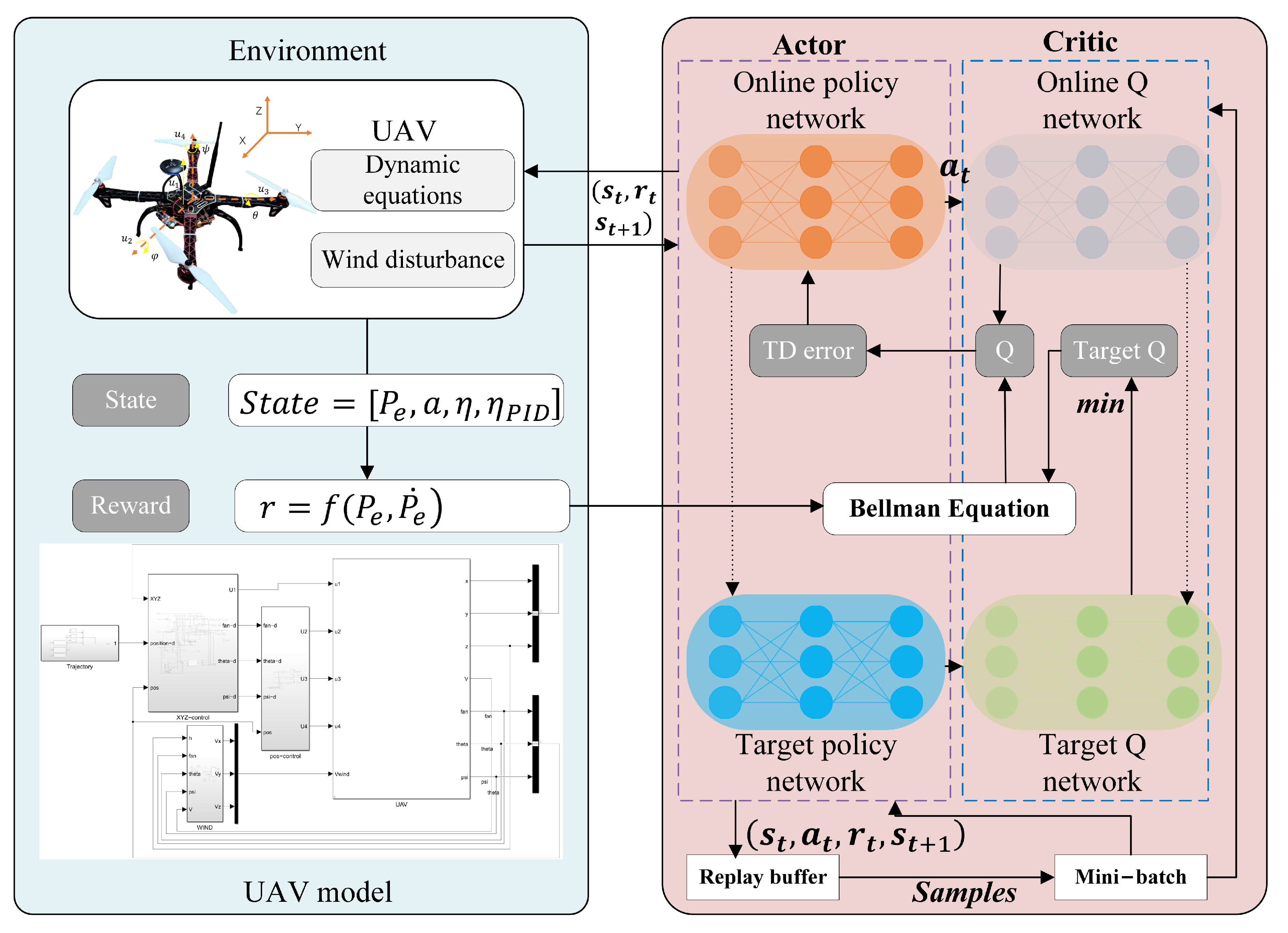
A DRL control strategy was employed for UAVs, with the DRL compensator utilizing interactions with the environment to learn the control strategy. Figure 3 illustrates the UAV model designed in this study and presents the framework of the DDPG-based DRL controller. The anti-disturbance control of UAVs presents a control challenge characterized by a high-dimensional continuous state and continuous action, suitable for the Actor–Critic method based on a deterministic policy gradient. The construction of the UAV tracking control model utilizes a deep deterministic policy gradient (DDPG)-based algorithm.

In a deterministic strategy, an agent’s action corresponds one-to-one with the state, denoted as follows:

$$\begin{array}{cc}S\to A& a_i=\end{array}\mu \left(s_i{\left|\theta \right.}^{\mu }\right)$$

(5)

where $a_i$ denotes the decision action of the agent at i, $s_i$ denotes the state of the agent at i, and $\mu$ and $\theta$ are the parameters in the policy and policy network, respectively.

In order to address the issue of prediction inaccuracy caused by multiple iterations of the same value network, the DDPG algorithm incorporates the notion of a target network. The target network employs only the strategy network and the value network to compute returns, and its parameters are periodically updated using those of the other two networks.

$${\theta }_{Q_{\mathrm{t}}}\leftarrow \tau {\theta }_Q+\left(1-\tau \right){\theta }_Q$$

(6)

$${\theta }_{{\mu }_t}\leftarrow \tau {\theta }_{\mu }+\left(1-\tau \right){\theta }_{\mu }$$

(7)

where $\tau$ is the soft update weight; ${\theta }_{Q_t}$ and ${\theta }_{{\mu }_t}$ are the target evaluation network and target strategy network, respectively; and ${\theta }_Q$ and ${\theta }_{\mu }$ are the online evaluation network parameters and online strategy network parameters.

In the DDPG algorithm, the input to the goal network is the next state $S_{i+1}$, the goal actor network predicts the next action through the policy ${\mu }_t$, and the valuation of the action $y_i$ using the goal critic network is expressed as follows:

$$y_i=r_i+\gamma ·Q_t\left(S_{i+1},{\mu }_t\left(S_{i+1}\left|{\theta }_{{\mu }_t}\right|\right)\left|{\theta }_{Q_t}\right.\right)$$

(8)

where $\gamma$ denotes the value update weight.

In the DDPG algorithm, exploration of the environment is achieved by adding random noise N to the action:

$$a_t=a_i+N$$

(9)

Updating the critic network with mean square error (MSE):

$$L={\displaystyle \frac{1}{N}}\sum _i{\left(y_i-Q\left(S_i,a_i\left|{\theta }_Q\right.\right)\right)}^2$$

(10)

where the gradient of the update strategy of the actor network is

$$\begin{array}{c}{\nabla }_{{\theta }_{\mu }}\mu {|}_{S_{\mathrm{i}}}={\displaystyle \frac{1}{N}}\sum _i{\nabla }_{{\theta }_{\mu }}\mu {|}_{S_i}\\ ={\displaystyle \frac{1}{N}}\sum _i{\nabla }_{a}Q\left(S,a\left|{\theta }_Q\right.\right){|}_{S=S_i,a=\mu \left(S_i\right)}{\nabla }_{{\theta }_{\mu }}\mu \left(S\left|{\theta }_{\mu }\right.\right){|}_{S=S_i}\end{array}$$

(11)

The pseudocode flow of the DDPG algorithm is shown in Algorithm 1.

Algorithm 1 DDPG Algorithm

1: Randomly initialize the parameters ${\theta }_Q$ and ${\theta }_{\mu }$ of the critic network $Q(S,a|{\theta }_Q)$ and the actor network $\mu \left(S\right|{\theta }_{\mu })$. 2: Initialize the parameters ${\theta }_{Q_t}$ and ${\theta }_{{\mu }_t}$ of the target networks $Q_t$ and ${\mu }_t$, where ${\theta }_{Q_t}\leftarrow {\theta }_Q$, ${\theta }_{{\mu }_t}\leftarrow {\theta }_{\mu }$. 3: Initialize the experience pool R. 4: for episode = 1 to M do 5:    Initialize the random noise N. 6:    Initialize the environment and get the initial state. 7:    for $t=1$ to T do 8:      Execute actions according to the policy network and explore the noise: $a_t=\mu \left(S_t\right|{\theta }_{\mu })+N$. 9:      Execute action $a_t$, update the environment to obtain new state $S_{t+1}$ and reward $r_t$. 10:      Obtain $(S_t,a_t,r_t,S_{t+1})$ and save to the experience pool R. 11:      Random sampling of small batches of several data from the experience pool. 12:      Calculate target Q: $y_i=r_i+\gamma ·Q_t(S_{i+1},{\mu }_t\left(S_{i+1}\right|{\theta }_{{\mu }_t})|{\theta }_{Q_t})$. 13:      Updating Critic-Network with Minimizing Loss Function: $L={\displaystyle \frac{1}{N}}{\sum }_i{(y_i-Q(S_i,a_i|{\theta }_Q))}^2$. 14:      Update the Actor-Network based on the strategy gradient of the samples:      ${\nabla }_{{\theta }_{\mu }}{\mu |}_{S_i}={\displaystyle \frac{1}{N}}{\sum }_i{\nabla }_{a}Q(S,a|{\theta }_Q){{|}_{(S=S_i,a=\mu \left(S_i\right))}{\nabla }_{{\theta }_{\mu }}\mu \left(S\right|{\theta }_{\mu })|}_{(S=S_i)}$. 15:      Updating the target network: ${\theta }_{Q_t}\leftarrow \tau {\theta }_Q+(1-\tau ){\theta }_Q$, ${\theta }_{{\mu }_t}\leftarrow \tau {\theta }_{\mu }+(1-\tau ){\theta }_{\mu }$. 16:    end for 17: end for

The design of the reward function is an important part of DRL, and the reward function directly affects the training effect of the agent. In order to avoid the algorithm obtaining positive values for too long a period due to reward sparsity and to promote the training process, a staged training approach is adopted, and the specific training process and reward mechanism are formulated in (12).

In the early stage of training, the UAV’s ability to hover at a fixed height without wind disturbance is developed. The maximum allowable altitude error is set to 2 m, with rewards earned when the altitude error is less than 1 m and the rate of change in altitude error is less than 3 m per second. Subsequently, the complete wind field perturbation model is introduced to train fixed-height hovering and the maximum allowable error is reduced to 1 m; rewards are obtained when the error is confirmed to be less than 0.1 m, the rate of change in the error is less than 0, and the number of the initial training sets is set to be 2000. Finally, the UAV uses the agents obtained from the previous stage of training to conduct the training of trajectory tracking, and the training task is set to resist the wind perturbation and track the desired position, and the maximum allowable error is set to be 0.1 m. The single-step reward is set as follows:

$$r=\left\{\begin{array}{ll}50·(0.1-\left|p_e\right|)& \left|p_e\right|<0.1\\ 20·(0.1-\left|p_e\right|)\hfill & 0.1\le \left|p_e\right|<0.5\\ -200·\left|p_e\right|\hfill & \left|p_e\right|\ge 0.5\\ -400·{\dot{p}}_e\hfill & -0.5<{\dot{p}}_e<0\end{array}\right.$$

(12)

where $P_e$ represents the position error while $\dot{P_e}$ indicates its rate of change. Additionally, r denotes the reward, and t stands for the runtime.

For each training set, the total reward is calculated as the sum of rewards from individual training steps, with the cumulative reward resetting to zero when the UAV initiates a new training set.

2.3. Wind Disturbance Rejection Control Strategy

To enhance the UAV’s robustness against wind disturbances, we introduce a wind disturbance rejection control strategy that integrates a dual-loop PID trajectory tracking controller with a DRL compensator. This strategy is designed to address trajectory errors caused by wind disturbances, ensuring effective trajectory tracking performance.

Dual-Loop PID Controller: Our control strategy employs a dual-loop PID controller, consisting of an outer position loop and an inner attitude loop. The outer loop controls the UAV’s position, while the inner loop manages its attitude. The PID controller adjusts the UAV’s position based on the error between the desired position and the actual position. This structure is crucial for achieving precise trajectory tracking.

DRL Compensator: The DRL compensator is trained on simulated wind fields based on fractal theory. It operates alongside the dual-loop PID controller, adapting to changing dynamics in response to wind disturbances. By leveraging historical wind data and simulating various wind scenarios, the DRL agent learns to predict the impact of wind on trajectory tracking. The DRL compensator analyzes trajectory errors generated by wind disturbances and adjusts the PID parameters in real time, effectively mitigating the lag effects commonly associated with pure PID control.

Training Process: The staged training approach allows the UAV to develop its capability to counter wind disturbances. Initially, the UAV learns to hover without wind, then is exposed to simulated wind conditions, refining its ability to maintain trajectory tracking under these circumstances.

Enhanced Performance: The integration of the DRL compensator with the dual-loop PID control scheme significantly mitigates the adverse effects of wind disturbances on trajectory tracking. The DRL compensator continuously adjusts PID parameters based on real-time observations, enhancing the overall responsiveness and stability of the UAV. This combined approach reduces tracking errors and improves robustness, enabling effective operation in varying wind environments.

2.4. Offshore Surface Wind Field Simulation Model

2.4.1. Composite Wind Field Modelling

A comprehensive wind field model based on atmospheric dynamics theory is developed to address wind disturbances [46]. The model captures the complexity of outdoor wind conditions by simulating various wind patterns, including real-time wind dynamics, wind shear, turbulence, and sudden changes in wind speed. By integrating these wind patterns into the training environment for the DRL compensator, the UAV is trained to effectively manage unpredictable wind disturbances and maintain stable flight.

$$V_{wind}=V_{shear}+V_{Dryden}+V_{gust}+V_{mean}$$

(13)

where, $V_{shear}$ denotes the wind shear model and the logarithmic wind shear model proposed by Prandtl [47] is used, and the model is represented as follows:

$$V_{shear}={\displaystyle \frac{V_{w0}}{k}}ln{\displaystyle \frac{H}{H_0}}$$

(14)

where $V_{shear}$ denotes the value of wind speed for wind shear, $H_0$ denotes the roughness height; H denotes the flight altitude; k denotes Karman’s constant; and $V_{w0}$ denotes the friction velocity, which is determined by the ground shear stress ${\tau }_0$ and the air density $\rho$, and is expressed as follows:

$$V_{w0}=\sqrt{{\displaystyle \frac{{\tau }_0}{\rho }}}$$

(15)

$V_{Dryden}$ is the turbulent wind based on the Dryden model [48], which is obtained from a large number of atmospheric turbulence statistics as follows:

$$\left\{\begin{array}{c}f\left(\xi \right)={\sigma }^{2}exp[-\xi /(L/v)]\\ g\left(\xi \right)=f\left(\xi \right)[1-\xi /(2L/v\left)\right]\end{array}\right.$$

(16)

where $f\left(\xi \right)$ is the longitudinal correlation function, $g\left(\xi \right)$ is the transverse correlation function, $\xi$ is the time variable, $\sigma$ is the turbulence intensity, L is the turbulence scale, and v is the airspeed.

$V_{gust}$ denotes a discrete sudden wind model using a half-wavelength discrete gust model [49] with the following model expression:

$$\left\{\begin{array}{ll}{V}_{gust}=0& x<0\\ V_{gust}={\displaystyle \frac{V_{w_m}}{2}}(1-cos{\displaystyle \frac{\pi x}{d_m}})\hfill & 0\le x\le d_m\\ V_{gust}=V_{w_m}\hfill & x>d_m\end{array}\right.$$

(17)

where $d_m$ denotes the gust scale range, $V_{w_m}$ denotes the peak gust, and x denotes the distance from the gust center.

$V_{mean}$ denotes the real-time wind speed measured by the UAV. Leveraging the fractal characteristics of wind speed time series, the time resolution of wind speed measurements is refined from hourly averages to per-second values. To enhance adaptability to real-world conditions, we replace the fixed wind speed values employed in previous studies with a dynamic fractal wind field model. This model is constructed using real-time, variable wind speed data collected from actual environments, ensuring that the UAV operates under more realistic, fluctuating wind conditions.

The fractal characteristics of the model allow it to simulate short-term bursts of strong winds and varying wind patterns, thereby accurately capturing the complexity of real-world environments.

2.4.2. Fractal Characterization and Validation of Wind Speed Time Series

In [50], the results of fractal analysis show that both daily and hourly mean wind speeds exhibit clear time series fractal behavior and the fractal dimension does not vary with time scale. Self-similarity is one of the important features of fractals, and when an object has self-similarity, then its fractal can be considered to have scale-invariance under geometric transformation, i.e., similarity or statistical self-similarity between time series under different time scales such as daily, weekly, and monthly [51]. Wind is a natural motion formed by the flow of air with apparent chaotic characteristics, and the wind speed time series exhibits obvious self-similarity. Therefore, the analysis of wind speed mapping based on wind speed time series data can be conducted using fractal analysis. The Hurst index is used to quantify the degree of fractal self-similarity in the time series and the persistence of the underlying stochastic process. Different Hurst indices correspond to different characteristics of the time series [52].

Several methods can be used to estimate the Hurst index, including the absolute value method, the aggregated variance method, the period gram method, and the rescaled range analysis R/S method. Among them, the R/S analysis method is a non-parametric analysis method, which makes few other assumptions about the object under examination and has good robustness [53]. The object of R/S analysis includes not only normal distribution, but also independent processes with non-Gaussian distribution, such as t, $\gamma$, $\Gamma$, and other distributions. The basic principle of R/S analysis is as follows:

$${\left({\displaystyle \frac{R}{S}}\right)}_{\mathrm{n}}=C·n^H$$

(18)

where R denotes the extreme deviation of the time series, S is the standard deviation, n is the time interval, C is a constant, and H is the Hurst index.

The R/S analysis method is to define a time series $\left\{R_t\right\}$ of length N, divide it into $A=\left[{\displaystyle \frac{T}{N}}\right]$ subsequences of length n, where the symbol $\left[\right]$ denotes rounding, and define each subinterval as $I_a$, where $a=1,2,...,A$. Any point in $I_a$ is denoted as $R_{k,a}$, $k=1,2,...,n$, $a=1,2,...,A$.

• Calculate individual subinterval means:

  $$R_a={\displaystyle \frac{1}{n}}\sum _{k=1}^n{r}_{k,a}$$

  (19)
• Calculate the cumulative mean deviation for individual subintervals:

  $$X_{k,a}=\sum _{i=1}^k(r_{k,a}-R_a)$$

  (20)
• Work out the extreme deviation of a single subinterval:

  $$R_{Ia}=\underset{k}{max}\left\{X_{k,a}\right\}-\underset{k}{min}\left\{X_{k,a}\right\}$$

  (21)
• Analyze the standard deviation of each subinterval:

  $$S_{Ia}=\sqrt{{\displaystyle \frac{1}{n}}\sum _{k=1}^n{(r_{k,a}-R_a)}^2}$$

  (22)
• Find the average rescaled extreme deviation of A subintervals of length n:

  $${\left(R/S\right)}_n={\displaystyle \frac{1}{A}}\sum _{a=1}^A{\displaystyle \frac{R_{Ia}}{S_{Ia}}}$$

  (23)
• Increase the value of n and repeat the above steps to obtain a series of $(n,{(R/S)}_n)$, which is obtained by taking the logarithm of (10)

  $$ln{(R/S)}_n=Hln\left(n\right)+c$$

  (24)

  where c is a constant, $ln\left(n\right)$ is the independent variable, $ln{(R/S)}_n$ is the dependent variable using the least squares method of linear fitting, and the slope of the resulting straight line is the estimated value of the Hurst index.

A relationship exists between the Hurst index and the fractal dimension D as follows:

$$D=2-H$$

(25)

According to fractal theory, the Hurst exponent of a time series ranges from 0 to 1, with different characteristics at different intervals, critical at 0.5.

• When $H=0.5,D=1.5$, the time series exhibits characteristics of a standard random wandering series. Data points are independent, lacking any correlation with each other. The time series of wind speeds conforms to a normal distribution, and wind speeds exhibit independence across all time scales. Furthermore, past and present data exert no influence on the future state.
• When $0.5<H\le 1$, $1\le D<1.5$, the time series has persistence, and if the series shows an increasing (decreasing) trend in the past, it will continue to maintain that increasing (decreasing) trend. The change in time scale will not affect the change in time series correlation, in which the value of H tends to be about 1; the greater the strength of the persistence of the time series, the lower the random component. The Hurst index is 1, which indicates that the time series has the ability to be completely predictable.
• When $0\le H<0.5$, $1.5<D\le 2$, the original series has anti-persistence; if the series in the past shows a rising (falling) state, the future period of time the series will show a falling (rising) state. The closer the value of H tends to be to 0, the greater the strength of the anti-persistence of the time series, and the lower the random component.

Therefore, the R/S analysis method shows excellent predictive ability in time series research by calculating the Hurst index of the time series and performing significance analysis. Specifically, by studying the change rule of the Hurst index and the significance index, the scale invariance of the wind speed time series is used to explore the change rule of the wind speed in different time scales and realize the relevant applications.

The pseudocode for the computation of the Hurst exponent for a sequence of arbitrary length $(n\ge 8)$ is shown in Algorithm 2.

Algorithm 2 Hurst Index Calculation Process

1: Input: $X=\{X_1,X_2,\cdots ,X_n\}={\left\{T{s}^k\right\}}_{1\le k\le n,n\ge 8}$ 2: Output: H 3: while True do 4:    Calculate the mean value R of the sequence X: $R_a={\displaystyle \frac{1}{n}}{\sum }_{k=1}^n{r}_{k,a}$ 5:    Calculate the cumulative mean deviation $\left\{X_{k,a}\right\}$: $X_{k,a}={\sum }_{i=1}^k(r_{k,a}-R_a)$ 6:    Work out individual sub-interval extremes $R_{I,a}$: $R_{I,a}=max\left\{X_{k,a}\right\}-min\left\{X_{k,a}\right\}$ 7:    Analyse the sub-interval standard deviation $S_{I,a}$: $S_{I,a}=\sqrt{{\displaystyle \frac{1}{n}}{\sum }_{k=1}^n{(r_{k,a}-R_a)}^2}$ 8:    Find the rescaled range sequence ${(R/S)}_n$: ${(R/S)}_n={\displaystyle \frac{R_{I,a}}{S_{I,a}}}$ 9:    if $n<4$ then 10:      break 11:    end if 12:    if $n\%2=0$ then 13:      $n\leftarrow n/2$ 14:      $X\leftarrow \left\{({\displaystyle \frac{(X_1+X_2)}{2}},{\displaystyle \frac{(X_3+X_4)}{2}},\cdots ,{\displaystyle \frac{X_{n-1}+X_n}{2}})\right\}$ 15:    end if 16:    if $n\%2\ne 0$ then 17:      $n\leftarrow n/2$ 18:      $X\leftarrow \{{\displaystyle \frac{(X_1+X_2)}{2}},{\displaystyle \frac{(X_3+X_4)}{2}},\cdots ,{\displaystyle \frac{X_{n-2}+X_{n-1}}{2}},X_n\}$ 19:    end if 20: end while 21: Fit the curve $ln{(R/S)}_n\sim ln\left(n\right)$ and calculate its slope to get H

2.4.3. Hurst Index Test Method

Typically, multifractal behavior in time series can be attributed to two main factors: long-range correlations within the data and the underlying probability distribution of the time series [54]. Thus, the technique of data rearrangement is employed to disturb the correlation within the data while preserving the probability density distribution of the original sequence.

To verify the validity of the long-range correlation of the wind speed time series, the wind speed time series is randomly perturbed and processed as follows:

• Randomly generate pairs of natural numbers $(i,j)$ of length less than N.
• Exchange the ith and jth data points in the wind speed time series $\left\{R_t\right\}$.
• Repeat the above steps $100N$ times to ensure adequate disruption of the data.
• Compute the Hurst index of the rearrangement sequence $\left\{R_{t_1}\right\}$.

When the multifractal behavior of the sequence $\left\{R_t\right\}$ is solely linked to its long-range correlation, the Hurst exponent of the rearranged sequence should be 0.5 after eliminating the correlation. If the multifractal behavior of the original sequence is only related to its probability density, the Hurst exponents of the original and the rearranged sequences should remain the same. If the multifractal behavior of the original sequence is influenced by both its long-range correlation and probability density distribution, the Hurst exponent of the rearranged sequence should satisfy $H\ne 0.5$, and the Hurst exponent of the rearranged sequence should be smaller than that of the original sequence.

In the significance test for the Hurst exponent, the null hypothesis is set as an independent and identically distributed stochastic process following a normal distribution, and its significance is determined by rejecting the null hypothesis. According to the literature [55], the following empirical formula is proposed:

$$E\left({\displaystyle \frac{R}{S_N}}\right)=\left({\displaystyle \frac{N-0.5}{N}}\right){{\displaystyle \frac{N\pi }{2}}}^{-0.5}\sum _{r=1}^{N-1}\sqrt{{\displaystyle \frac{N-r}{r}}}$$

(26)

where the corresponding $E(R/S_N)$ when N takes different values was calculated, respectively, and a linear fit was made to $ln\left(N\right)$ and $ln\left(E(R/S_N)\right)$, whose slopes were taken as the expected value of the Hurst exponent, $E\left(H\right)$. Then, the corresponding significance test formula was as follows:

$$l={\displaystyle \frac{H-E\left(H\right)}{\sqrt{1/T}}}$$

(27)

In the $5\%$ significance level test, the null hypothesis is accepted when $\left|\lambda \right|<1.96$, indicating that the time series is a standard stochastic wandering series with randomness. Conversely, the null hypothesis of randomness is rejected when $\left|\lambda \right|>1.96$. In such cases, the time series is deemed persistent when $\lambda >1.96$, and conversely, it is considered anti-persistent when $\lambda <-1.96$.

2.5. Flight Experiment Design

In order to verify the wind field model and controller control effect proposed in this paper, flight experiments were carried out in simulation and real environments, respectively, with the following specific scheme.

2.5.1. Simulation Experimental Design

In the simulation environment, two scenarios were designed: one with no wind disturbance and the other with composite wind field disturbance. The composite wind field continuously generates simulated wind conditions, in which the composite wind speed exceeds 10 m/s. The data of fractal wind speed and composite wind speed are shown in Figure 4a,b, respectively. The aim is to thoroughly investigate the robust control capabilities of the controller under wind field perturbations to ensure that the UAV maintains stability effectively.

The trajectory tracking experiment aims to assess the stability performance of the UAV regarding attitude and altitude in the presence of wind field perturbations. The UAV takes off from point A and follows the boundary of the operation area following the cow ploughing curve pattern, as depicted in Figure 4c. Upon reaching the boundary, the UAV turns and moves laterally by width d to continue the operation, repeating this process until completing the cow ploughing curve to point B. The mean is obtained to examine the stability of the UAV in hovering, straight-line flight, flight around the point, and large-curvature turns.

Using the MATLAB/Simulink platform, various modules of the UAV are built for simulation and modelling. The traditional PID algorithm controller is selected as the method control.

2.5.2. Real-World Flight Experiment Design

The experimental setup, as shown in Figure 5, comprises a quadcopter UAV designed to test the robustness and feasibility of the proposed control algorithm under wind disturbances. The platform includes several key modules: a flight computer for control calculations, a quadcopter frame, power motors, brushless electronic speed controllers, a flight controller, a GPS module, and a wireless data transmission unit. The CUAV V5+ flight controller is the core of the system, responsible for executing the proposed PID-DRL control model. This controller receives feedback on the UAV’s flight state (velocity, position, and attitude angles) and calculates control commands for the motors. The flight controller communicates with the ground control station via a serial port utility to receive remote commands and execute corresponding tasks.

To provide a clearer overview of the UAV’s hardware components and their specifications,

Table 2. UAV hardware configuration.

Component	Specification
Flight Controller	CUAV V5+, STM32F765 processor
IMU Sensor	ICM-20602/ICM-20689/BMI055
Power Motors	DJI 2212 920 KV brushless self-locking motors
Electronic Speed Controller	SKYWALKER-20A
GPS Module	CUAV NEO V2
Telemetry Unit	CUAV P9 wireless data transmission unit
Total Mass (m)	0.65 kg
Inertia ($I_{xx}$, $I_{yy}$, $I_{zz}$)	0.0075 kg · m2, 0.0075 kg · m2, 0.013 kg · m2
Gravitational Acceleration (g)	9.8 N/kg
Arm Length (l)	0.23 m
Lift Coefficient (b)	$3.1\times {10}^{-5}$ N · s2

summarizes the key elements that make up the experimental platform.

The proposed PID-DRL-based control model runs on the CUAV V5+ flight controller. The controller is equipped with an STM32F765 main processor and an IMU sensor model ICM-20602/ICM-20689/BMI055, which can measure key flight state parameters with high precision. The UAV’s total lift is generated by four DJI 2212 920 KV brushless motors, with rotational speed controlled by SKYWALKER-20A electronic speed controllers. Real-time position data are obtained through the GPS module CUAV NEO V2, and experimental data are transmitted to the local host via CUAV P9 telemetry.

Additionally, the UAV experimental platform and control structure framework is shown as follows: The speed of the brushless motors is regulated in real time by the output pulse-width modulation (PWM) signal. The torque control of the UAV is achieved by adjusting the rotational speed of the symmetrically placed power motors on the frame. Horizontal torque is generated on the UAV frame when the speed of neighboring power motors is varied. When the rotational speed of the relative power motors is changed, a vertical torque is generated on the UAV frame, and the attitude angle of the UAV varies with the change in the torque on the frame. In the above manner, the UAV can track a predetermined desired trajectory in a timely manner based on real-time data.

The UAV developed in this study is designed for high-precision and stable flight in outdoor wind field environments. An open and windy location was chosen for the experiment, with real-time wind speeds estimated based on the day’s wind warning information. In order to further verify the reliability of the control algorithm proposed in this study, the wind-resistant and stabilizing flight mode is introduced in the real world using the constructed UAV platform for experimental analysis according to the requirements of the actual flight mission.

3. Results and Discussion

In order to evaluate the control effectiveness of the proposed PID-DRL perturbation compensation controller in dynamic environments, the following experiments, hardware-in-the-loop simulation experiments and physical flight tests, were designed and conducted. The control effect evaluation index is based on two criteria, root mean square error (RMSE) and maximum tracking index (MAX), providing a quantitative assessment of the control performance, and the evaluation equations are as follows:

$$\begin{array}{cc}RMSE=\sqrt{{\displaystyle \frac{1}{N}}{\displaystyle \sum _{i=1}^N}{e}_{pos\_xyz\_i}^2}& \hspace{1em}\hspace{1em}\forall i\in A\end{array}$$

(28)

$$MAX=max\left(\left|e\left(i\right)\right|\right)$$

(29)

where N denotes the sample capacity and $e_{pos\_xyz\_i}$ denotes the trajectory tracking error.

3.1. Fractal Characterization of Wind Speed Time Series

This paper uses the measured wind speed time series data from an area in eastern China, sourced from the “Wave and Wind Data” released by the National Marine Science Data Centre, as an illustrative example. The time series dataset calculates the hourly average wind speed based on 10 min sampling intervals. Covering one year, the dataset has a resolution of 1 h, resulting in a total of 8928 data points.

The selected wind speed time series were subjected to R/S analysis, and the Hurst index was calculated using Python programming, and validity and significance analyses were performed. Taking the wind speed time series data in October 2022 as an example, the original wind speed series and the R/S analysis results are shown in Figure 6.

• The plot of $log(R/S)$ against $log\left(n\right)$ exhibits a strong linear relationship in double logarithmic coordinates, and the slope of the least-squares fitting curve for $log(R/S)$ against $log\left(n\right)$ represents the Hurst exponent of the wind speed time series for that month. The calculated Hurst exponent is $H=0.315$, and this value falls within the range of $0\le H<0.5$.
• Instances in the time series are randomly disrupted and rearranged, and the result of the R/S analysis for the time series after rearranging indicates $H=0.16$. This value falls within the range of $0\le H<0.5$.
• The test of significance was performed according to (19), and the instances satisfy $\lambda =-6.71<-1.96$, which passes the $95\%$ confidence level test.

The presented results affirm that the outcome of $0\le H<0.5$ at a $95\%$ confidence level is not attributed to error but rather objectively reflects the inherent characteristics of the wind speed time series. This verification indicates that the wind speed time series in October exhibits clear fractal characteristics, pointing to its self-similarity across various time scales.

The outcomes of the R/S analysis for the annual wind speed time series at this site are presented in

Table 3. R/S analysis and significance analysis results.

Month	Hurst	Fractal Dimension	Significance Indicator	Hurst (Rearranged)	Significance (Rearranged)
1	0.261	1.739	−8.213	0.122	−11.807
2	0.322	1.678	−6.870	0.103	−12.823
3	0.233	1.767	−9.282	0.169	−11.035
4	0.272	1.728	−8.126	0.110	−12.490
5	0.275	1.725	−8.147	0.141	−11.811
6	0.168	1.832	−10.922	0.134	−11.846
7	0.281	1.719	−7.991	0.107	−12.720
8	0.271	1.729	−8.175	0.128	−12.024
9	0.195	1.805	−10.342	0.134	−11.998
10	0.315	1.685	−6.710	0.162	−10.620
11	0.318	1.682	−6.905	0.101	−12.718
12	0.282	1.718	−7.968	0.161	−11.258
Mean	0.266	1.734	−8.304	0.131	−11.930

.

Table 3 reveals that the Hurst indices of the wind speed time series at this site span the range of 0–0.5 throughout the year, and all of these indices have undergone successful significance verification. This indicates the presence of long-range correlation in the measured wind speed time series at this site, with the long-range correlation reflecting anti-persistence characteristics. Furthermore, it confirms that the wind speed time series at this site exhibits a certain degree of scalar invariance across different time scales.

Post rearranging the disrupted data, the Hurst index for the wind speed time series data for the entire year exhibits a notable reduction, indicating that the time series data lacs true independence, and disrupting the order of the data compromises the structure of the system. Additionally, the Hurst index for the wind speed time series after the rearrangement satisfies $H\ne 0.5$, suggesting that the fractal characteristics of the time series are associated with its probability density distribution. Furthermore, the Hurst index of the rearranged sequence is significantly smaller than that of the original sequence, concluding that the fractal characteristics of the wind speed time series result from the combined influence of its probability density distribution and its long-range correlation.

Based on the results from the R/S analyses of wind speed time series over the past year, it is clear that the observed wind speeds at the selected wind farms exhibit typical fractal characteristics and scale invariance, as outlined in this paper.

3.2. Reinforcement Learning Controller Training Results

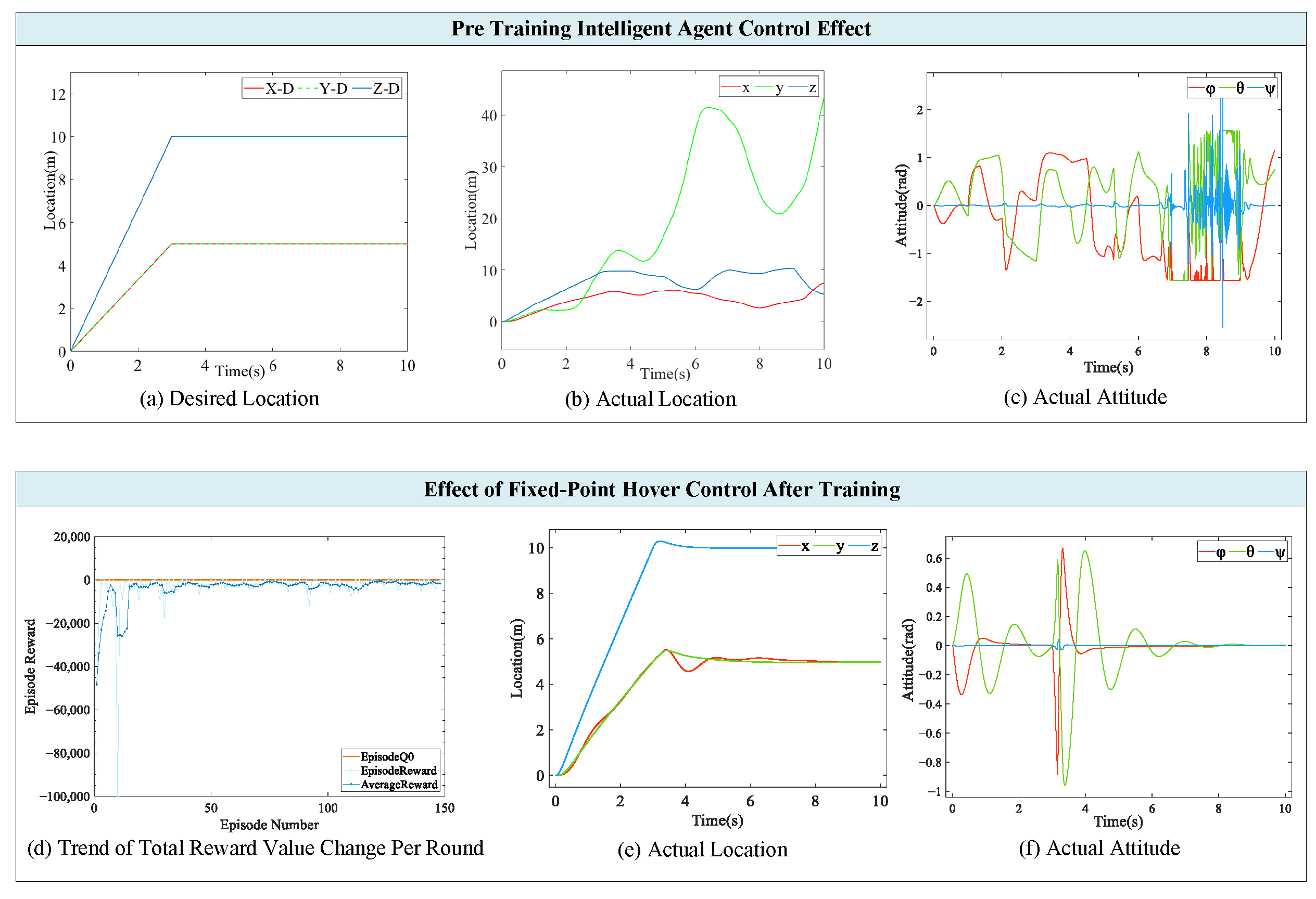
Figure 7b shows the exploration stage of the agent, with the desired position depicted in Figure 7a. Since the training learning through the neural network has not been carried out at this time, the agent is incapable of controlling the UAV to achieve fixed-point hovering under windless working conditions.

Figure 7d shows the trend of the reward system obtained by the agent action per round. Figure 7e,f depict the trends of the UAV position and attitude angle after training. In the early stages of the training process, the rewards obtained in rounds exhibit large fluctuations, with the minimum value reaching about $-5\times {10}^4$. This is attributed to the extensive stochastic exploration undertaken by the agent due to the lack of experience in executing a reasonable action in a certain deterministic state. In the later stages of training, the round reward increases and stabilizes with the rise in training rounds, and the fluctuation gradually decreases. This suggests that the agent has more effectively achieved the exploration and exploitation of actions, ultimately learning the control strategy for fixed-point hovering.

To verify the trajectory tracking ability of the trained agent under wind disturbance, the trajectory is designed, as depicted in Figure 8a. As shown in Figure 8b,c, it is evident that although the agent trained in the previous stage can achieve the trajectory tracking effect to a certain extent, it shows obvious jitter in the late stage of trajectory tracking after 80 s. This jitter raises concerns about potential overheating and damage to the UAV motors. During trajectory tracking, the agent experiences significant fluctuations in the attitude angle, with a maximum change exceeding 0.8 radians, which poses a risk of UAV capsize under wind disturbances. In summary, to address the observed issues, further training is conducted to enhance the agent’s trajectory tracking performance.

As shown in Figure 8d, the reward value obtained in each round at the beginning of training exhibits fluctuating characteristics. Considering that the trajectory tracking task is more complex compared to the fixed-point hovering task, the duration of the fluctuating rounds is also longer. As the number of training rounds increases, the fluctuation in the reward value gradually decreases, signifying that the agent can explore and apply actions more effectively. However, the reward value jumps and fluctuates in part of the rounds, indicative of the phenomenon where the action space of the agent is over-explored. Upon further increasing the number of iterations, the reward value gradually converges, and the fluctuation in the reward value diminishes after 300 rounds, suggesting that the UAV trajectory tracking control model based on the DDPG algorithm is approaching convergence. The agent has successfully learned an effective trajectory tracking control strategy.

3.3. Simulation Experiment Results and Discussion

The simulation results and the control system performance indices are presented in Figure 9 and

Table 4. Performance indicators for wind-disturbance-free stability testing.

	POX_X $\mathit{e}\left(\mathit{m}\right)$	POX_Y $\mathit{e}\left(\mathit{m}\right)$	POX_Z $\mathit{e}\left(\mathit{m}\right)$	$\mathit{\varphi }$ (Attitude_ABS)	$\mathit{\theta }$ (Attitude_ABS)	$\mathit{\psi }$ (Attitude_ABS)
PID	0.9	1.6	0.6	0.65	1.08	0.024
PID_DRL	0.5	0.7	0.3	0.96	1.17	0.11
PID_DRL_T	0.4	0.6	0.3	1.03	1.16	0.09

below.

No wind disturbance:

Here, e denotes the amount of overshoot; PID, PID_DRL, and PID_DRL_T, respectively, represent pure PID control, untrained PID_DRL controller, and PID-DRL controller trained in stages; and Attitude_ABS represents the maximum value of the corresponding attitude angle change. Significant differences are observed in the wind-turbulence-free stability test, with PID_DRL_T, in particular, demonstrating a lower level of overshooting. This controller reduces the amount of overshooting by 55.6% (POS_X), 62.5% (POS_Y), and 50% (POS_Z), resulting in reductions in the maximum values of $\varphi$ and $\theta$ by 8.5% and 4.6%, respectively. Taking into account both the amount of overshooting and the attitude angle control, PID_DRL_T exhibits superior overall performance compared to PID and PID_DRL. However, it is important to note that some attitude jitter is introduced along with the improved response speed.

In the given experimental setup, it is noteworthy that the PID controller demonstrates notable performance in a windless environment. More precisely, the PID controller shows relatively stable height control in the POS_Z axis and satisfactory performance in the POS_X and POS_Y axes. This suggests that the PID controller is effective in meeting job requirements under windless conditions. However, the differing control effects observed in the X and Y axes can be attributed to the need to accommodate varying wind speeds in these directions during wind disturbance scenarios. The PID parameters were specifically tuned to address the higher wind perturbations encountered along the X axis, ensuring effective trajectory tracking and stability. Hence, when choosing the most suitable controller, considering the performance indicators and integrating them with the actual application cases ensures that the selected controller can meet the work requirements by maintaining stability and improving efficiency.

In the trajectory tracking experiment, the initial attitude angle and altitude of the UAV are 0. The UAV trajectory tracking response curve is shown in Figure 10a.

An extensive quantitative analysis of the graphical results yields the following outcomes: There are significant disparities in XY-plane trajectory tracking under windless conditions among the three controllers (PID, PID_DRL, and PID_DRL_T). Both the PID and PID_DRL_T controllers exhibit superior performance in trajectory tracking, outperforming the RMSE values and maximum error (MAX) of the untrained PID_DRL controller.

Specifically, the PID controller presents a significant advantage in achieving the desired trajectory. In terms of RMSE values, the PID and PID_DRL_T controllers show similar trends and have a maximum value of about 0.2, respectively, whereas the maximum value of the PID controller is smaller than that of the PID_DRL_T controller, and both are significantly smaller than that of the untrained PID_DRL controller, which fluctuates with a mean value of about 0.6 and a peak value of more than 1.2.

The trends in maximum error (MAX) align with those observed in the RMSE values. In the absence of wind, both the PID controller and PID_DRL_T controller exhibit similar control, with the PID controller demonstrating a MAX of approximately 0.18, and the PID_DRL_T controller exhibiting a MAX of 0.32—both significantly smaller than the untrained PID_DRL controller.

In summary, the PID controller demonstrates superior performance in trajectory tracking under windless conditions, whereas the trained PID_DRL controller closely approaches the performance of the PID controller and outperforms the untrained PID_DRL controller by a significant margin. The use of a traditional PID controller in windless conditions can reduce the controller computational load and improve control efficiency while ensuring effective control.

With composite wind field disturbance:

The experimental results and control performance indices are shown in Figure 11.

Quantitatively analyzing the trajectory tracking performance, we can see that PID_DRL_T achieves significant improvements compared to PID, which can be contextualized against existing solutions in UAV control systems.

• Visualization of Trajectory Tracking Effect: Upon examining the XY-plane trajectory projection (Figure 11a), it is evident that the trajectory tracking effect of PID_DRL_T closely resembles that of PID under wind disturbances. However, during the take-off and landing phases, PID_DRL_T exhibits slightly smoother control with less error fluctuation compared to PID. Notably, the trajectory projection curve of PID_DRL_T is consistently enclosed within the PID curve throughout the entire trajectory, indicating its superior trajectory tracking effect. This aligns with the growing need for enhanced UAV performance in environments affected by dynamic wind conditions.
• Quantitative Percentage Improvement: In terms of specific data, two key performance indicators were focused on, namely RMSE (root mean square error) and maximum error (Max). The comparison results are as follows:

Concerning RMSE, the RMSE peak of PID_DRL_T is reduced by approximately 30% compared to PID, decreasing from 0.58 m to 0.42 m. The sub-wave peak is approximately 0.45 m at around 70 s for PID_DRL_T, while for PID, the sub-wave peak is about 0.38 m at around 37 s. In comparison to the untrained PID_DRL controller, the mean RMSE of PID_DRL_T is reduced by approximately 65%, decreasing from 0.8 m to 0.28 m, and the peak RMSE is also reduced by about 67%, decreasing from 1.38 m to 0.44 m.

Concerning the maximum error (Max), the maximum error of PID_DRL_T is reduced by approximately 36% compared to PID, decreasing from 0.44 m to 0.28 m. In comparison to the untrained PID_DRL controller, the maximum error of PID_DRL_T is reduced by about 65%, decreasing from 0.8 m to 0.28 m.

The percentage improvement underscores the substantial superiority of the PID_DRL_T approach over traditional PID control in terms of trajectory tracking performance, particularly in challenging wind conditions. Research on the wind resistance capabilities of multi-rotor UAVs has focused on mitigating wind disturbances under high-wind conditions, with studies demonstrating the ability to withstand winds of up to 16 m/s [36], often using static wind models. In contrast, the approach that leverages real-time wind data to train the PID-DRL controller provides a more dynamic response, allowing the UAV to adapt its control strategy to varying wind environments.

Notably, the effectiveness of the trained PID_DRL_T controller highlights the critical role of training in enhancing control effectiveness and stability. While the wind resistance capabilities of UAVs are commonly assessed through induced velocity and propeller thrust metrics [19], the proposed method goes further by incorporating learning-based adaptive control strategies that effectively handle both horizontal and gusty winds. The innovative approach not only offers a new solution for UAVs facing wind disturbances but also significantly improves operational efficiency in real-world scenarios, ultimately enhancing the UAV’s stability against wind disturbances through continuous adaptation of the agent model and control strategy.

3.4. Real-World Flight Experiments

Figure 12 shows the experimental circumstances and the outcomes of the aerial test conducted on the specified day. The experimental platform transitions into the wind-resistant and stabilization flight mode immediately after lift-off and conducts hovering (b) and trajectory tracking tests (c) under the depicted weather and wind conditions (a). In this mode, the reinforcement learning compensator contributes to control. As depicted in the curves of (b), the UAV achieves precise hovering at the specified position with an attitude angle change of less than 0.3 rad using the proposed control algorithm. Furthermore, in the trajectory tracking test, the UAV demonstrates excellent performance, with the maximum attitude angle change not exceeding 0.27 rad, along with minimal fluctuations and jumps. These are primarily attributed to the control algorithm’s resistance to external wind perturbations, showcasing the UAV’s robustness and adaptability in this flight mode. Through these flight tests, the control algorithm’s exceptional performance in trajectory tracking and hovering, along with its strong adaptability, is validated on the real platform.

3.5. Novelty and Limitations

The innovation resides in the establishment of an original reference framework for the fractal characteristics of temporal wind speed time series, facilitating adaptation to real-time wind speed variations within the composite wind field model. Through the utilization of the DDPG algorithm for reinforcement learning, stable hovering and high-precision trajectory tracking control of a UAV under wind field disturbance are achieved.

This work developed a comprehensive wind field model by integrating turbulent wind, shear wind, and abrupt changes in wind components. Integrating real-time wind speed data into the wind field model improves its accuracy and simulation efficacy, establishing a dependable basis for controller development.

To enhance the control performance of the UAV in the presence of wind disturbances, a reinforcement learning methodology was employed. Through the utilization of the DDPG algorithm and training in simulated wind conditions, acquired control strategies were effectively applied to maneuver the UAV with stability and execute predetermined flight paths even in complex wind situations. To expedite the learning process and minimize the duration of training, a segmented learning approach was adopted.

There are still several limitations that need to be addressed in future work. One of the primary issues is the system’s limited ability to adapt to rapidly changing wind fields, which require a higher temporal resolution for accurate real-world wind simulation. To overcome this, future efforts will focus on collecting wind speed data with higher time resolution, which will optimize and refine the wind field model. A comprehensive analysis of the fractal characteristics of these high-resolution wind data will also be conducted to further improve accuracy, efficiency, and safety in the UAV’s anti-wind-disturbance performance.

Additionally, we plan to develop a virtual environment with a simulated wind field. This will involve the creation of a simulation engine-based wind field model to enhance the visualization and effectiveness of wind field simulations. These improvements aim to create more realistic and intuitive scenarios for testing, enabling a more thorough evaluation of the UAV’s performance under diverse wind conditions.

Furthermore, future tests will assess the effectiveness of the trained controllers and UAVs in higher wind speeds and more complex, realistic wind field models. This analysis will provide deeper insights into the UAV’s wind stability in challenging environments. By adjusting various configurations of the experimental platform, we will explore how hardware influences the system’s performance under wind disturbances. This approach will offer valuable insights for optimizing both the control strategies and the experimental platform for future applications.

4. Conclusions

In short, this study suggests a trajectory tracking controller for a UAV in severe wind conditions, using a combination of PID control and DRL. In order to account for the fluctuations in wind speed in the wind field model, a model is proposed that utilizes fractal theory. The Hurst exponent is derived using the R/S analysis method to ensure the importance and usefulness of the fractal characteristics and scale invariance. The DRL compensator is trained and substantially enhances the trajectory tracking control effect by utilizing the wind speed time series model. The experimental results further confirm the efficacy of the PID-DRL controller.

• In stable weather conditions, the traditional PID controller can effectively model the dynamics of unmanned aerial vehicles (UAVs). Using classic PID controllers in windless situations guarantees efficient control and decreases the computational load on the controller, improving total control efficiency.
• The selected annual wind speed time series underwent validation through R/S analysis, revealing a Hurst index below 0.5, indicative of its anti-persistence feature. Through meticulous validation assessing the significance and validity of the Hurst index, it was confirmed that the time series indeed possesses distinct fractal characteristics. This confirmation solidifies its scale invariance across various time scales, providing robust support for the fitting of real-time wind speeds across different time scales.
• The trained PID_DRL_T controller demonstrates a noteworthy improvement in performance compared to the untrained PID_DRL controller, indicating that the training scheme, grounded in wind speed time series, effectively improves the trajectory tracking control effectiveness of the agent, which provides useful empirical support for exploring the precise handling of UAVs under different operating conditions.