UAV Anomaly Detection Method Based on Convolutional Autoencoder and Support Vector Data Description with 0/1 Soft-Margin Loss

Abstract

Unmanned aerial vehicles (UAVs) are becoming more widely used in various industries, raising growing concerns about their safety and reliability. The flight data of UAVs can directly reflect their flight health status; however, the rarity of abnormal flight data and the spatiotemporal characteristics of these data represent a significant challenge for constructing accurate and reliable anomaly detectors. To address this, this study proposes an anomaly detection framework that fully considers the temporal correlations and distribution characteristics of flight data. This framework first combines a one-dimensional convolutional neural network (1DCNN) with an autoencoder (AE) to establish a feature extraction model. This model leverages the feature extraction capabilities of the 1DCNN and the reconstruction capabilities of the AE to thoroughly extract the spatiotemporal features from UAV flight data. Then, to address the challenge of adaptive anomaly detection thresholds, this research proposes a nonlinear model of support vector data description (SVDD) utilizing a 0/1 soft-margin loss, referred to as L0/1-SVDD. This model replaces the traditional hinge loss function in SVDD with a 0/1 loss function, with the goal of enhancing the accuracy and robustness of anomaly detection. Since the 0/1 loss function is a bounded, non-convex, and non-continuous function, this paper proposes the Bregman ADMM algorithm to solve the L0/1-SVDD. Finally, the difference between the reconstructed and the actual value is employed to train the L0/1-SVDD, resulting in a hypersphere classifier that is capable of detecting UAV anomaly data. The experimental results using real flight data show that, compared with methods such as AE, LSTM, and LSTM-AE, the proposed method exhibits superior performance across five evaluation metrics.

1. Introduction

In recent years, as electronics, sensors, and communication technologies have continually advanced, unmanned aerial vehicles (UAVs) have been widely used in various fields, including emergency search and rescue, crop protection, logistics, aerial photography, news reporting, crop management, and crop yield prediction [1,2,3,4,5]. UAVs offer advantages, such as being lightweight, compact, easy to carry, and capable of operating in extreme environments, thus helping humans to complete specific tasks. However, as the complexity of UAV systems and the diversity of their missions continue to increase, the UAV accident rate has also been on the rise in recent years. These accidents have resulted in significant economic losses. To reduce the risk of accidents involving UAVs in commercial, medical, and other application scenarios, it is crucial to conduct anomaly detection research on UAVs to promptly identify and isolate anomalies [6,7].

With the growing use of UAVs in various application domains, extensive research has been conducted on anomaly detection in UAV flight data. Anomaly detection methods for UAVs can be broadly classified into three main categories: knowledge-based methods, model-based methods, and data-driven methods [7,8]. Knowledge-based methods rely on domain experts’ knowledge and experience to define and model the characteristics and attributes of normal UAV flight data to identify anomalies. The effectiveness of this approach depends heavily on the expertise and experience of the specialists involved, which can limit its adaptability. Model-based anomaly detection methods involve constructing mathematical models with which to simulate normal UAV flight behavior and detect anomalies based on the deviations between the model outputs and the actual observed data. This approach generally requires the development and optimization of UAV dynamic models, control system models, or physical behavior models. However, model-based methods depend on a comprehensive understanding and prior knowledge of the system, requiring significant domain knowledge and experience to establish accurate physical models. This can be challenging for complex flight data, limiting the applicability of such methods [9,10,11]. In contrast, data-driven methods do not rely on prior knowledge, but use machine learning and data mining techniques to automatically extract features from large amounts of data for anomaly detection. These methods are better suited to handle the diversity and complexity of data, making them an important research direction for anomaly detection.

Currently, many data-driven UAV anomaly detection methods identify anomalies through reconstruction errors and prediction errors, especially those based on deep learning [12]. Therefore, the threshold plays a crucial role in anomaly detection, as it indicates whether a fault condition truly exists within a system. Common thresholds in the existing research include the fixed threshold [13] and the parameter-dependent threshold [14]. The former sets a fixed global threshold, identifying the data exceeding this value as abnormal, while the latter defines a threshold using parameters such as the density or distance between data points, deeming faults to have occurred if the threshold is exceeded. Due to the diversity and dynamic nature of UAV sensor faults, these two threshold methods do not adequately meet the requirements for UAV anomaly detection.

To address the aforementioned issues, a method combining deep neural networks with classification techniques can be employed, using reconstruction errors and prediction errors for classification. SVDD is considered a highly effective classification method for identifying anomalies, but it is susceptible to the outliers and noise present in the training datasets [15]. Since reconstruction and prediction errors may contain outliers, directly applying the SVDD method to anomaly detection can significantly impact the detection accuracy. Statistical analysis indicates that the binary loss function is among the most suitable loss functions used in machine learning. It minimizes classification error rates to the greatest extent and exhibits strong robustness against outliers and label noise. Wang et al. proposed a new 0/1 non-convex approximate-loss SVM, which improved the accuracy and robustness of the SVM algorithm [16,17]. Therefore, this research introduces a UAV anomaly detection algorithm that utilizes the 0/1 loss function of the SVDD combined with a convolutional autoencoder (CAE-L0/1-SVDD). The primary contributions of this study can be outlined as follows:

(1)

We developed a convolutional autoencoder (CAE) model incorporating a 1DCNN and an AE, which merges the feature extraction strengths of the 1DCNN with the reconstruction abilities of the AE to obtain the spatiotemporal features from the data.

(2)

Given the non-convex nature and the challenges of solving the 0/1 loss function directly, we introduce the Bregman ADMM method into the L0/1-SVDD model.

(3)

To address the issue of poor adaptability when manually determining thresholds based on reconstruction errors, the difference between the reconstructed values and the actual values of the UAV data is input into the L0/1-SVDD threshold determination module for secondary training. As a result, an optimal threshold is obtained, which improves the recall, detection, and accuracy rates.

(4)

The effectiveness of the proposed approach is assessed using actual flight data. The evaluation validates the proposed method’s effectiveness and demonstrates its superior performance compared to existing approaches to UAV anomaly detection.

The rest of this paper is structured as follows: Section 2 discusses the theoretical foundations of AEs and SVDDs. Section 3 describes the proposed UAV anomaly detection method. Section 4 provides an analysis of the experimental findings obtained from applying the proposed method to real datasets. Section 5 concludes with a summary of the key findings and contributions of this research, along with suggestions for future work.

2. Related Work

Data-driven anomaly detection methods use machine learning and data mining techniques to automatically extract features from large datasets for anomaly detection. These methods typically include traditional machine learning approaches and deep learning methods. Due to the limited availability of labeled data and the rarity of abnormal samples in UAV flight data, traditional machine learning methods, such as K-means clustering, one-class support vector machines (OC-SVM), kernel principal component analysis (KPCA), decision trees, and local outlier factor (LOF), have been widely used for anomaly or fault detection in UAV flight data [18,19]. While these methods are effective in certain scenarios, they are insensitive to changes in data trends, struggle to handle complex time series data, and have limited feature extraction capabilities. Moreover, they suffer from high computational complexity and low efficiency when dealing with high-dimensional data. Lu-Kai Song et al. [20] proposed a cascade ensemble learning method that combines the cascade synchronous strategy with wavelet neural network-based AdaBoost ensemble learning, and applied it to the reliability analysis and anomaly detection of aeroengine turbine rotor systems.

Deep learning techniques have demonstrated strong capabilities in feature extraction and anomaly detection, particularly in handling complex data patterns. Through automated feature learning mechanisms, deep learning models can capture the underlying complex relationships and patterns of large, high-dimensional datasets, leading to their widespread application in UAV anomaly detection [21,22,23,24]. Deep learning-based anomaly detection is primarily divided into two theoretical approaches: reconstruction-based methods and prediction-based methods. The reconstruction-based approach assumes that abnormal data will result in more significant reconstruction errors compared to normal data, while the prediction-based approach assumes that abnormal data will exhibit more significant prediction errors [25,26]. Zhong et al. developed an LSTM-based method that leverages the spatiotemporal correlations to achieve anomaly detection and fault recovery for fixed-wing UAVs [27]. Chang et al. developed a fault-tolerant adaptive control approach using the LSTM technique to achieve stable and rapid attitude control, effectively addressing the challenges posed by high dynamic disturbances and surface failures in fixed-wing UAVs [28]. Wang and others [29,30], recognizing the difficulties in obtaining accurate physical models of UAVs and the presence of random noise, as well as the spatial and temporal correlations within flight data, designed an LSTM-based regression model that extracts the spatiotemporal features from flight data and uses filters to smooth the residuals between the actual flight data and estimated values, achieving good anomaly detection results. Guo et al. [31] integrated UAV flight action modes and actuator state information to develop an LSTM-based fault detection model that enables the efficient detection of actuator faults under dynamic flight conditions through a comparison with the corresponding detection thresholds. Park et al. [32] trained a stacked autoencoder (SAE) model using only normal data, where the reconstruction loss was used to distinguish between the safe and fault states. G. Jiang et al. [33] used an LSTM autoencoder (LSTM-AE) to simultaneously detect UAV anomalies and network attacks. Bell and others designed an LSTM–stacked autoencoder (LSTM-SAE) for UAV anomaly detection [34,35].

3. Preliminaries

3.1. Autoencoder

The autoencoder (AE) represents a well-known model in the domain of unsupervised deep learning neural networks. It consists of multiple, nonlinear processing layers designed to learn the distribution features and representations of nonlinear data. The structure of the autoencoder, as shown in Figure 1, comprises two main components: an encoding layer and a decoding layer [36]. The encoding layer transforms the input features into a compact representation, preserving the essential data characteristics and removing unnecessary details from the features, while maximizing the retention of essential information in the features. This is computed through the following formula:

$$H=\phi \left(W_e\chi +b_e\right)$$

(1)

where $\chi$ denotes the input data, $H$ indicates the features in the latent space, $\phi$ is the activation function, $b_e$ denotes the bias matrix for the encoding layer, and $W_e$ represents the weight matrix of the encoding layer. The decoding layer aims to understand the features in a reduced dimensional space and reconstruct them to match the original input with the following computation formula:

$$\widehat{\chi }=f\left(W_{d}H+b_d\right)$$

(2)

where $\widehat{\chi }$ is the output data after the AE computation, $f$ is the activation function, $b_d$ is the bias matrix for the decoding layer, and $W_d$ is the weight matrix for the decoding layer. The goal of an AE model is to reduce the discrepancy between the input data and its reconstructed output, enabling the AE to recover the original input features. The following formula illustrates this calculation:

$$R_{\left(\chi -\widehat{\chi }\right)}=\arg \min f_L\left(\chi ,\widehat{\chi }\right)$$

(3)

where $R_{\left(\chi -\widehat{\chi }\right)}$ represents the reconstruction error of the AE model and $f_L$ denotes the reconstructed loss function.

3.2. SVDD

SVDD is a data description method based on statistical principles. Its core idea is to find the smallest possible hypersphere that maximally encompasses the target data while keeping the non-target data outside the hypersphere [37]. The problem formulation is outlined below:

$$\begin{array}{l}\underset{R,\mu ,{\xi }_i}{\min } R^2+C_1{\displaystyle \sum _{i\in I^{+}}{\xi }_i}+C_2{\displaystyle \sum _{j\in I^{-}}{\xi }_j}\\ \mathrm{s}.\mathrm{t} {‖\phi \left(x_j\right)-\mathrm{a}‖}^2\ge R^2-{\xi }_j, {\xi }_j>0, j\in I^{-}\\ \hspace{1em}{‖\phi \left(x_i\right)-\mathrm{a}‖}^2\le R^2+{\xi }_i, {\xi }_i>0,i\in I^{+}\end{array}$$

(4)

where $\mathrm{a}$ represents the center of the hypersphere, $R$ represents the radius of the hypersphere, $C_1$ and $C_2$ are coefficients for penalizing the slack variables, and ${\xi }_i$, ${\xi }_j$ denote the slack variables. By using the Lagrange multiplier method, the dual problem can be formulated as

$$\begin{array}{l}\max L\left(\alpha \right)={\displaystyle \sum _i{\alpha }_i{y}_i\left(x_i\cdot x_i\right)}-{\displaystyle \sum _{i,j}{\alpha }_i{\alpha }_j{y}_i{y}_j\left(x_i\cdot x_j\right)}\\ \mathrm{s}.\mathrm{t} {\displaystyle \sum _i{\alpha }_i{y}_i=1}, 0\le {\alpha }_i\le C_{y_i}, \mathrm{for} i=1,\cdots ,n\end{array}$$

(5)

where ${\alpha }_i$ is the Lagrange multiplier, and $y_i\in \left\{+1,-1\right\}$, such that $y_i=1$ for samples from the target class and $y_i=-1$ for samples from the non-target class. According to the KKT condition, the center and radius of the hypersphere are given by

$$\mathrm{a}={\displaystyle \sum _{i=1}^n{\alpha }_i}{y}_i\phi \left(x_i\right)$$

(6)

$$R=‖\phi \left(x_{sv}\right)-\mathrm{a}‖=\sqrt{\left(x_{sv}\cdot x_{sv}\right)-2{\displaystyle \sum _i{\alpha }_i{y}_i\left(x_{sv}\cdot x_i\right)}+{\displaystyle \sum _{i,j}{\alpha }_i{\alpha }_j{y}_i{y}_j}\left(x_i\cdot x_j\right)}$$

(7)

where $x_{sv}$ represents the support vectors.

When the test sample $z$ is received, its decision function is defined as

$$f\left(z\right)=R^2-{‖z-\mathrm{a}‖}^2=R^2-\left(z\cdot z\right)+2{\displaystyle \sum _i{\alpha }_i{y}_i\left(z\cdot x_i\right)}-{\displaystyle \sum _{i,j}{\alpha }_i{\alpha }_j}{y}_i{y}_j\left(x_i\cdot x_j\right)$$

(8)

If $f\left(z\right)\ge 0$, the sample $z$ is classified as belonging to the target class; otherwise, it is identified as a non-target class sample.

4. Algorithm Framework

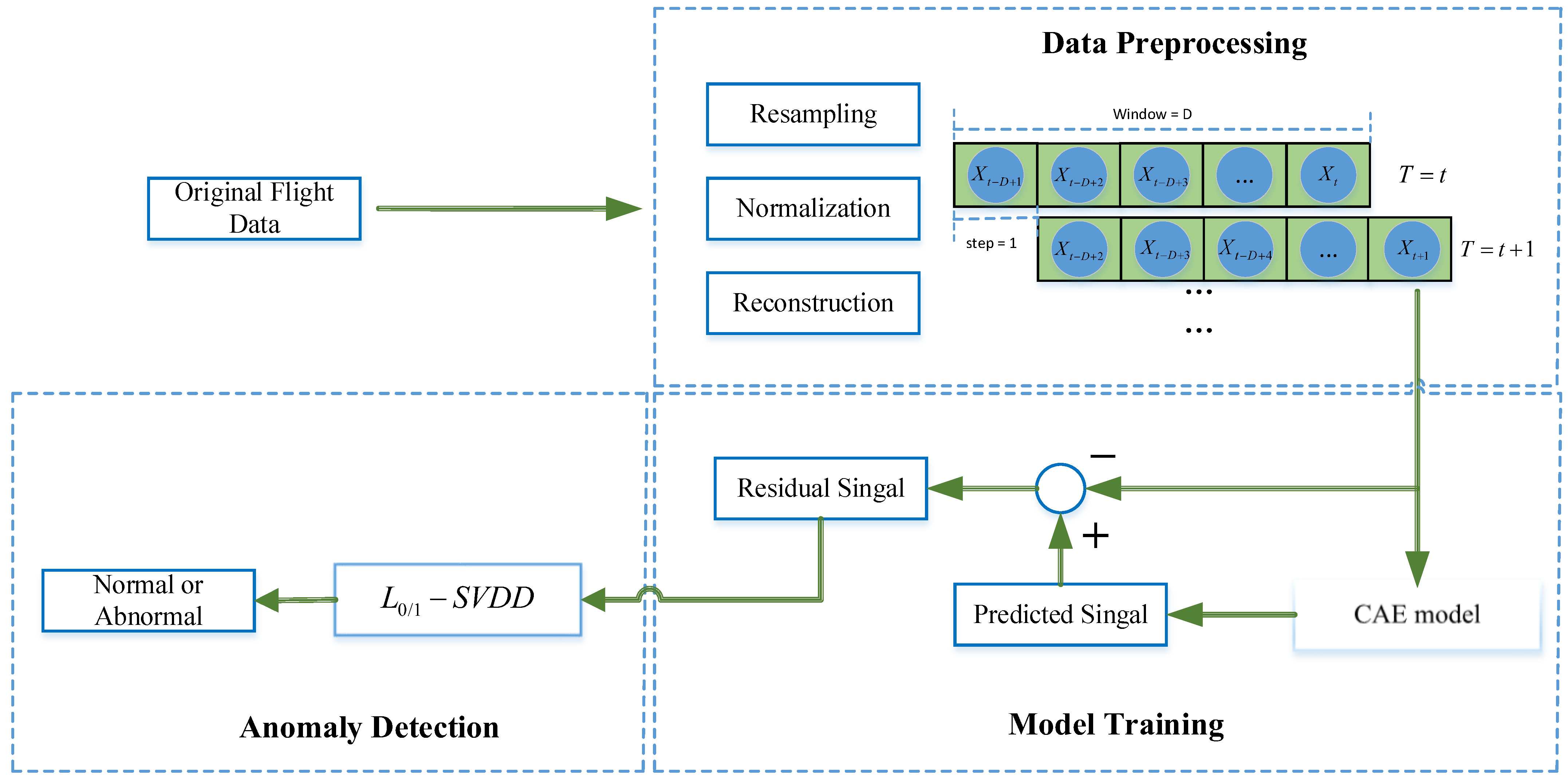
This study proposes a novel anomaly detection framework designed to detect various anomalies in UAVs. Figure 2 shows the overall structure of the proposed anomaly detection framework, which consists of three main steps. The first step involves preprocessing the flight data, which includes tasks such as resampling, normalization, and reconstruction using a sliding window. After feature engineering, the preprocessed flight data are split into training and testing datasets. The training and validation sets contain only normal flight data, while the testing set includes anomalous flight data. In the second stage, the preprocessed training data are employed to develop and assess the CAE model, with residuals obtained by contrasting the input data with the reconstructed data. Finally, the residual signals are used to train the L0/1-SVDD model, which is employed to predict anomalies within the residuals.

4.1. Data Preprocessing

Due to the varying measurement units, parameter ranges, and sampling frequencies of UAV sensor characteristics, it is necessary to preprocess these feature parameters before performing anomaly detection. In this study, the following three preprocessing operations were carried out.

(1)

Resampling: Since the sampling frequencies of the selected features are inconsistent, the data are resampled at a frequency of 10 Hz.

(2)

Normalization: To ensure that the input UAV feature data are on the same scale, the input data are normalized. The Z-score technique is employed to standardize the data, and it is expressed as follows:

$$Z_{Data}={\displaystyle \frac{X_{Data}-mean\left(X_{Data}\right)}{std\left(X_{Data}\right)}}$$

(9)

where $Z_{Data}$ is the normalized value, $X_{Data}$ is the feature data, $mean\left(X_{Data}\right)$ is the mean of the data, and $std\left(X_{Data}\right)$ is the standard deviation of the data. This formula transforms the data into standardized values having a mean equal to zero and a standard deviation of one.

(3)

Reconstructing flight data: To fully utilize the temporal correlations in UAV data, this study adopts a sliding window approach to reconstruct the flight data. Assuming that there are $N$ sampling points, the flight data representation is given by

$$X=\left[\begin{array}{cccc}{x}_{1,1}& x_{1,2}& \dots & x_{1,N}\\ x_{2,1}& x_{2,2}& \dots & x_{2,N}\\ ⋮& ⋮& \dots & ⋮\\ x_{m,1}& x_{m,2}& \dots & x_{m,N}\end{array}\right], x_{i,j}\in R$$

(10)

where $m$ indicates the total number of features. By setting the sliding window length and the stride to 1, the reconstructed data at time $t$ are formulated as

$${\tilde{X}}_{t-Window}=\left[\begin{array}{cccc}{x}_{1,t-Window+1}& x_{1,t-Window+2}& \dots & x_{1,t}\\ x_{2,t-Window+1}& x_{2,t-Window+2}& \dots & x_{2,t}\\ & \dots & & \\ x_{m,t-Window+1}& x_{m,t-Window+2}& \dots & x_{m,t}\end{array}\right]$$

(11)

The reconstructed flight data are expressed in the form:

$${\tilde{X}}_R=\left[\begin{array}{cccc}{\tilde{X}}_{1-Window}& {\tilde{X}}_{2-Window}& \dots & {\tilde{X}}_{N-Window}\end{array}\right]$$

(12)

4.2. Model Training

4.2.1. CAE Model

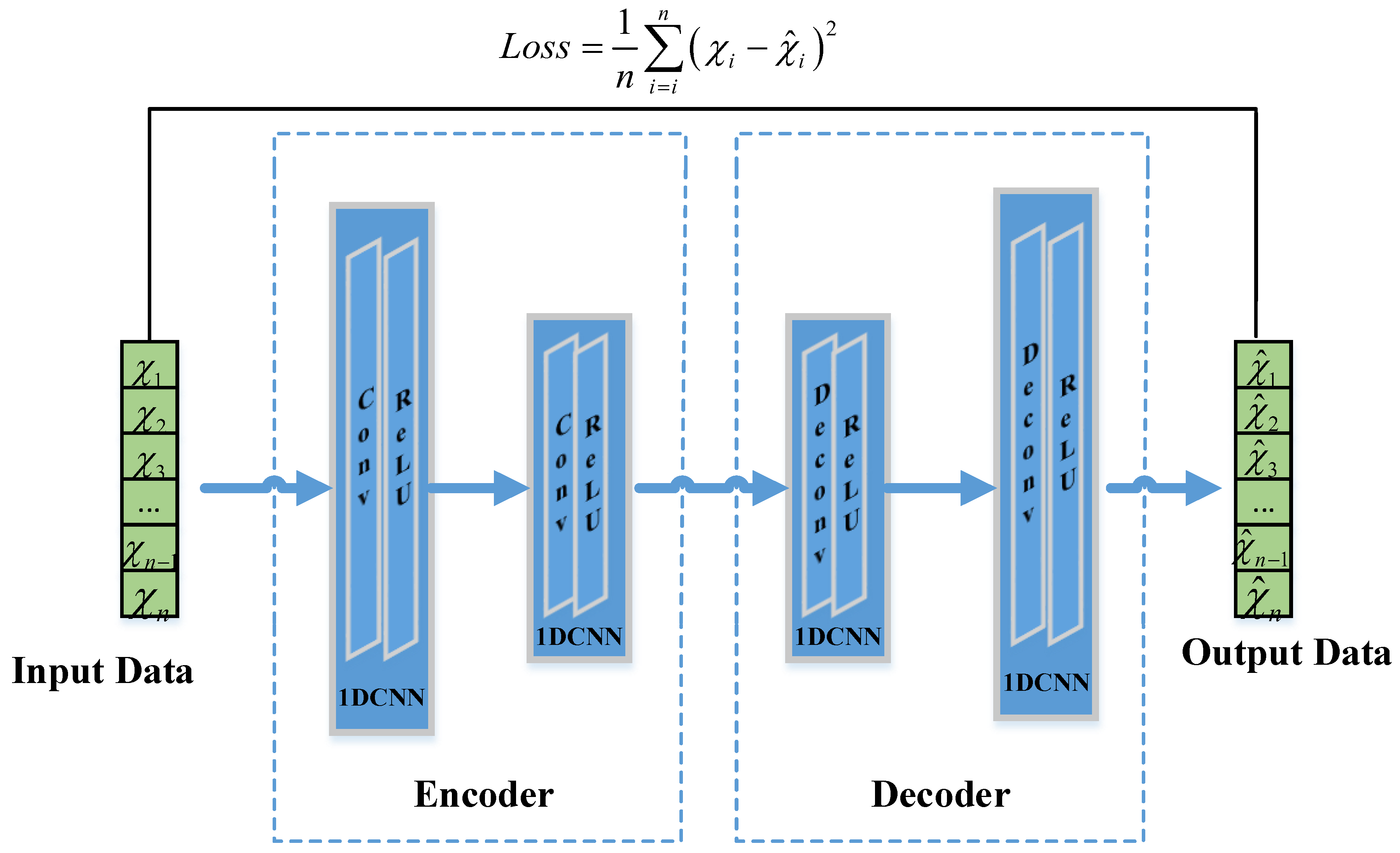
The CAE model is a neural network that uses 1DCNNs as the encoder–decoder layers, combined with linear layers. It leverages the reconstruction capability of the AE, the feature extraction ability of the 1DCNN, and the mapping ability of the linear layers on the data to efficiently extract the spatiotemporal features. Figure 3 shows the architecture of the CAE model, where two 1DCNNs are used as encoding layers to extract the spatial features, the linear layers perform mapping at the temporal level, and, finally, two 1DCNNs are used as decoding layers to reconstruct the features in the latent space.

Assuming that the flight data after preprocessing are $X$, the input data undergo feature extraction by the first convolutional layer in the encoding stage. The 1DCNN calculates the feature values between the samples using a sliding convolutional kernel, effectively capturing the feature relationships between the samples. A 1DCNN includes a convolutional layer and an activation layer. The flight data are subjected to feature extraction by the first 1DCNN in the encoding stage, and the encoder’s computation is defined by the following equation:

$$z_j^c=f\left(b_j^c+{\displaystyle \sum _{m=1}^M{W}_{m,j}^c*x_m^{c-1}}\right)$$

(13)

where $z_j^c$ denotes the resulting feature corresponding to the $j\mathrm{th}$ channel with the $c\mathrm{th}$ convolutional layer; $b_j^c$ is the bias for the $j\mathrm{th}$ feature; $W_{m,j}^c$ denotes the convolutional weight matrix; $M$ represents the input channel data; $*$ denotes the convolution operation; the term $x_m^{c-1}$ refers to the feature map from the $m\mathrm{th}$ input channel with the $c\mathrm{th}$ convolutional layer, capturing the channel’s data input; and $f$ denotes the ReLU activation function. In the encoding stage, there are two 1DCNN layers, and the convolution operation in the second layer is the same as in Equation (13). Thus, the latent space feature matrix is obtained after the encoding stage.

The decoder part of the CAE contains two 1DCNN layers, where each 1DCNN includes a deconvolution (transposed convolution) layer and an activation layer. In the decoding stage, the latent space is reconstructed into data with the same window size, and the decoding process can be expressed by the following calculation:

$${\widehat{x}}_j^c=f\left({\widehat{b}}_j^c+{\displaystyle \sum _{m=1}^M{\widehat{W}}_{m,j}^c\odot z_m^{c-1}}\right)$$

(14)

where ${\widehat{x}}_j^c$ represents the output feature corresponding to the $j\mathrm{th}$ channel with the $c\mathrm{th}$ deconvolution layer; ${\widehat{b}}_j^c$ indicates the bias associated with the $j\mathrm{th}$ feature; ${\widehat{W}}_{m,j}^c$ denotes the convolutional weight matrix; $M$ represents the input channel data; and $\odot$ denotes the deconvolution operation.

Training the model requires iteratively adjusting the weight parameters via backpropagation to reduce the disparity between the reconstructed and input data. The aim of the model’s training in this study is defined by the following objective function:

$$Loss={\displaystyle \frac{1}{n}}{\displaystyle \sum _{i=1}^n{\left(X_i-{\widehat{X}}_i\right)}^2}$$

(15)

4.2.2. Time Complexity of CAE Model

The time complexity of the CAE model primarily depends upon the computational cost of the 1D convolution and deconvolution (or transposed convolution) operations. A 1D CAE is typically used for processing one-dimensional sequence data and consists of two main components: the encoder and the decoder. The following sections will detail the time complexity of the encoder and decoder.

(1)

Time Complexity of the Encoder

The time complexity of the encoder is primarily determined by the 1D convolutional layers. Let us suppose the encoder has $d$ 1D convolutional layers, with the following parameters for each layer:

$L_i$: Length of the input sequence for the $i\mathrm{th}$ convolutional layer.

$C_{in,i}$: Number of input channels (features) for the $i\mathrm{th}$ convolutional layer.

$C_{out,i}$: Number of output channels (number of filters) for the $i\mathrm{th}$ convolutional layer.

$K_i$: Size of the convolution kernel (filter length) for the $i\mathrm{th}$ convolutional layer.

$S_i$: Stride of the deconvolution.

$P_i$: Padding size.

The output sequence length for the $i\mathrm{th}$ convolutional layer is

$$L_{out,i}={\displaystyle \frac{L_i+2P_i-K_i}{S_i}}+1$$

(16)

The time complexity for a single convolutional layer involves computing the convolution for each output position, which includes an element-wise multiplication and sum. Thus, the time complexity for the $i\mathrm{th}$ layer is

$$O\left(L_{out,i}{K}_i{C}_{in,i}{C}_{out,i}\right)$$

(17)

The total time complexity for the encoder is the sum of the time complexities of all the convolutional layers:

$$T_{encoder}=O\left({\displaystyle \sum _{i=1}^d\left(\frac{L_i+2P_i-K_i}{S_i}+1\right)K_i{C}_{in,i}{C}_{out,i}}\right)$$

(18)

(2)

Time Complexity of the Decoder

The decoder uses 1D deconvolution (or transposed convolution) operations to reconstruct the input sequence. The output sequence length for the $j\mathrm{th}$ deconvolutional layer is

$${L^{\prime }}_{out,j}=S_j\left(L_j-1\right)+K_j-2P_j$$

(19)

The time complexity for a single deconvolutional layer is similar to that of a convolutional layer:

$$O\left({L^{\prime }}_{out,j}{K}_j{C}_{in,j}{C}_{out,j}\right)$$

(20)

Supposing that the decoder has $d^{\prime }$ deconvolutional layers, the total time complexity for the decoder is the sum of the time complexities of all the deconvolutional layers:

$$T_{decoder}=O\left({\displaystyle \sum _{j=1}^{d^{\prime }}{L^{\prime }}_{out,j}{K}_j{C}_{in,j}{C}_{out,j}}\right)$$

(21)

(3)

Time Complexity of the CAE

The overall time complexity of the 1D convolutional autoencoder is the sum of the time complexities of both the encoder and the decoder:

$$T=T_{encoder}+T_{decoder}$$

(22)

Upon substituting the expressions for the encoder and decoder, we obtain

$$T=O\left({\displaystyle \sum _{i=1}^d{L}_{out,i}{K}_i{C}_{in,i}{C}_{out,i}}\right)+O\left({\displaystyle \sum _{j=1}^{d^{\prime }}{L^{\prime }}_{out,j}{K}_j{C}_{in,j}{C}_{out,j}}\right)$$

(23)

The time complexity of the 1D convolutional autoencoder is influenced by several factors: the number of convolutional and deconvolutional layers, where having more layers increases the computational complexity; the size of the convolution and deconvolution kernels, with larger kernels requiring more computations; the number of input and output channels, where having more channels adds to the complexity of each operation; and the stride and padding, where smaller strides lead to higher complexity due to more computations, and the padding increases the input size, further raising the computations required.

4.3. Anomaly Detection Based on L0/1-SVDD

4.3.1. The L0/1-SVDD Model

Based on the representer theorem [38], a set of vectors $\alpha$ can be found, such that the expression for the center $\mathrm{a}={\displaystyle \sum _{i=1}^n{\alpha }_i}{y}_i\phi \left(x_i\right)$ represents the optimal solution for Equation (4). Substituting $\mathrm{a}={\displaystyle \sum _{i=1}^n{\alpha }_i{y}_i}\phi \left(x_i\right)$ into Equation (4) yields

$$\begin{array}{l}\underset{a,R}{\min } R^2+C{\displaystyle \sum _{i=1}^{n}L\left({\xi }_i\right)}\\ {\xi }_i=y_i{K}_{ii}+y_i{\displaystyle \sum _{j=1}^n{\displaystyle \sum _{k=1}^n{y}_j{a}_j{y}_k{a}_k{K}_{jk}-y_i{R}^2}}-2y_i{\displaystyle \sum _{j=1}^n{y}_j{a}_j{K}_{ij}}\end{array}$$

(24)

where $K_{ij}=K\left(x_i,x_j\right)$ and $L$ is the loss function.

The 0/1 loss function is

$$L_{0/1}\left(u\right)={‖u_{+}‖}_0=\left\{\begin{array}{cc}1\hfill & u>0\hfill \\ 0\hfill & u\le 0\hfill \end{array}\right.$$

(25)

According to Equation (25), it can be seen that when $u>0$, $L_{0/1}\left(u\right)=1$; otherwise, $L_{0/1}\left(u\right)=0$. The 0/1 loss function creates a clear hard boundary by strictly distinguishing between correct and incorrect classifications. This strict boundary reduces the model’s sensitivity to outliers, resulting in a more robust decision boundary. Since the 0/1 loss function focuses only on whether a classification is correct, without considering the magnitude of the deviation, it makes the SVDD more robust when dealing with noisy data. Even in the presence of noise points, the 0/1 loss function does not significantly increase the loss due to the noise, thereby reducing interference with the model’s decision boundary. This gives the 0/1 loss function excellent robustness.

By replacing $L$ in Equation (24) with $L_{0/1}$, the L0/1-SVDD model can be expressed as

$$\underset{R,{\alpha }_y}{\min } R^2+C{L}_{0/1}\left(K_I+a_y^{T}K{a}_{y}Y-2K_D{a}_y-R^{2}Y\right)$$

(26)

The above notations are defined as

$$\begin{array}{l}{K}_I={\left(y_1{K}_{11},y_2{K}_{22},\dots ,y_n{K}_{nn}\right)}^T\in {ℝ}^{n\times 1}\\ K_D=\left[y_1{K}_{1·},y_2{K}_{2·},\dots ,y_n{K}_{n·}\right]\in {ℝ}^{n\times n}\\ Y={\left(y_1,y_2,\dots ,y_n\right)}^T\in {ℝ}^{n\times 1}\\ a_y={\left(y_1{a}_1,y_2{a}_2\dots ,y_n{a}_n\right)}^T\in {ℝ}^{n\times 1}\\ C=\left(c_{y_1},c_{y_2}\dots ,c_{y_n}\right)\in {ℝ}^{1\times n}\end{array}$$

(27)

The 0/1 loss function is characterized as bounded, non-convex, and discontinuous, with a zero gradient at its differentiable points, which complicates the process of solving this equation. In the following, this paper mainly discusses the solution of the L0/1-SVDD model. The Lagrangian function of Equation (26) is given by

$$L_{\lambda }\left(R^2,a_y,z,\lambda \right)=R^2+C{L}_{0/1}\left(z\right)+{\lambda }^T\left(K_I+a_y^{T}K{a}_{y}Y-2K_D{a}_y-R^{2}Y-z\right)$$

(28)

The KKT conditions for Equation (26) are provided below:

$$\left\{\begin{array}{c}\left(2Y{a}_y^{*T}K-2{K_D}^T\right){\lambda }^{{*}^T}=0\\ \partial C{L}_{0/1}\left(z^{*}\right)-{\lambda }^{*}∍0\\ K_I+a_y^{{*}^T}K{a}_y^{*}Y-2K_D{a}_y^{*}-R^{2^{*}}Y-{\lambda }^{*}=0\\ {\lambda }^{{*}^T}Y=1\end{array}\right.$$

(29)

where $\left(R^{2^{*}},a_y^{*},z^{*},{\lambda }^{*}\right)$ is a KKT point of Equation (26).

4.3.2. The Proximal Operator of $L_{0/1}$

Definition 1

(Proximal Operator) [39]. The proximal operator $pro{x}_{\lambda f\left(x\right)}$ for a closed convex function  $f\left(x\right)$ can be expressed by the following definition:

$$pro{x}_{\lambda f\left(x\right)}\left(x\right)=\arg \min \left\{{\displaystyle \frac{1}{2\lambda }}{‖y-x‖}^2+f\left(y\right)\right\}$$

(30)

The purpose of the proximal operator $pro{x}_{\lambda f\left(x\right)}$ is to find a point $y$ such that it not only minimizes the function $f\left(y\right)$, but also minimizes the distance between $y$ and $x$. The proximal operator is widely used in various optimization algorithms, especially in iterative solutions, where it is employed to handle non-differentiable or complex regularization terms. In this paper, the proximal operator is applied to manage the non-differentiable parts of the L0/1-SVDD model.

Lemma 1

[33]. For given parameters $\lambda >0$, $C>0$, the proximal operator of the $L_{0/1}$ is

$$pro{x}_{\lambda C{L}_{0/1}}\left(x\right)=\left\{\begin{array}{cc}0& 0\le x<\sqrt{2\lambda C}\\ 0 \mathrm{or} x& x=\sqrt{2\lambda C}\\ x& x>\sqrt{2\lambda C} \mathrm{or} x<0\end{array}\right.$$

(31)

4.3.3. Bregman ADMM Algorithm for L0/1-SVDD

Section 4.3.1 presents the mathematical optimization model for the L0/1-SVDD model. Due to the presence of a non-convex and non-continuous loss function in the optimization mathematical model, this paper employs the Bregman ADMM method to solve Equation (26). The augmented Lagrangian function for Equation (26) is given by the following expression:

$$L_{\mu }\left(R^2,a_y,z,\lambda ,\mu \right)=R^2+C{L}_{0/1}\left(z\right)+{\lambda }^T\left(f\left(a_y\right)-R^{2}Y-z\right)+{\displaystyle \frac{\mu }{2}}{‖f\left(a_y\right)-R^{2}Y-z‖}^2$$

(32)

where $\lambda \in {ℝ}^n$ denotes the Lagrange multiplier vector, $\mu >0$ indicates a penalty coefficient, and $f\left(a_y\right)=K_I+a_y^{T}K{a}_{y}Y-2K_D{a}_y$. Based on the values of $\left(R^{2^k},a_y^k,z^k,{\lambda }^k\right)$, the Bregman ADMM algorithm proceeds with the following iterative steps:

$$z^{k+1}=\underset{z\in {ℝ}^m}{\arg \min }{L}_{\mu }\left(R^{2^k},a_y^k,z,{\lambda }^k\right)$$

(33)

$$a_y^{k+1}=\underset{a_y\in {ℝ}^m}{\arg \min }{L}_{\mu }\left(R^{2^k},a_y,z^{k+1},{\lambda }^k\right)+\Delta D_{{\varphi }_1}\left(a_y,a_y^k\right)$$

(34)

$$R^{2^{k+1}}=\underset{R^2\in {ℝ}^m}{\arg \min }{L}_{\mu }\left(R^2,a_y^{k+1},z^{k+1},{\lambda }^k\right)+\Delta D_{{\varphi }_2}\left(R^2,R^{2^k}\right)$$

(35)

$${\lambda }^{k+1}={\lambda }^k+\mu \left(f\left(a_y^{k+1}\right)-R^{2^{k+1}}Y-z^{k+1}\right)$$

(36)

(1)

Updating $z^{k+1}$: According to Equation (30) and Equation (33), the solution of $z^{k+1}$ can be expressed as

$$\begin{array}{l}{z}^{k+1}=\underset{z\in {ℝ}^m}{\arg \min }C{L}_{0/1}\left(z\right)+{\displaystyle \frac{\mu }{2}}{‖\left(f\left(a_y^k\right)+{\displaystyle \frac{{\lambda }^k}{\mu }}-R^{2^k}Y\right)-z‖}^2\\ \hspace{1em} =\underset{z\in {ℝ}^m}{\arg \min }C{L}_{0/1}\left(z\right)+{\displaystyle \frac{\mu }{2}}{‖s^k-z‖}^2\\ \hspace{1em} =pro{x}_{{\displaystyle \frac{c}{\mu }}{L}_{0/1}}\left(s^k\right)\end{array}$$

(37)

where $s^k=f\left(a_y^k\right)+{\displaystyle \frac{{\lambda }^k}{\mu }}-R^{2^k}Y$.

(2)

Updating $a_y^{k+1}$

By analyzing Equation (34), it is evident that a closed-form solution for the variable $a_y^{k+1}$ cannot be obtained, requiring iterative computation, which results in a slower algorithm. To enhance the efficiency of solving the L0/1-SVDD model, we introduce an improved ADMM approach utilizing the Bregman distance.

The Bregman distance for a differentiable convex function $\varphi$ can be described by the following expression:

$$\Delta D_{\varphi }\left(y,x\right)=\varphi \left(y\right)-\varphi \left(x\right)-\left(\nabla \varphi \left(x\right),y-x\right)$$

(38)

In this paper, by setting $\varphi \left(x\right)={\displaystyle \frac{\beta }{2}}{‖x‖}^2-{\displaystyle \frac{\mu }{2}}{‖f\left(x\right)+{\displaystyle \frac{{\lambda }^k}{\mu }}-R^{2^k}Y-z^{k+1}‖}^2$, the Bregman distance $\Delta D_{\varphi }\left(y,x\right)$ is obtained as

$$\begin{array}{l}\Delta D_{{\varphi }_1}\left(y,x\right)={\displaystyle \frac{\beta }{2}}{‖y-x‖}^2-{\displaystyle \frac{\mu }{2}}{‖f\left(y\right)+{\displaystyle \frac{{\lambda }^k}{\mu }}-R^{2^k}Y-z^{k+1}‖}^2+{\displaystyle \frac{\mu }{2}}{‖f\left(x\right)+{\displaystyle \frac{{\lambda }^k}{\mu }}-R^{2^k}Y-z^{k+1}‖}^2\\ \hspace{1em}\hspace{1em}\hspace{1em}+〈\mu \nabla f\left(x\right)\left(f\left(y\right)+{\displaystyle \frac{{\lambda }^k}{\mu }}-R^{2^k}Y-z^{k+1}\right),y-x〉\end{array}$$

(39)

Substituting Equation (39) into Equation (34) yields

$$\begin{array}{l}{a}_y^{k+1}=\underset{a_y\in {ℝ}^m}{\arg \min }{\displaystyle \frac{\beta }{2}}{‖a_y-a_y^k‖}^2+{\displaystyle \frac{\mu }{2}}{‖f\left(a_y^k\right)+{\displaystyle \frac{{\lambda }^k}{\mu }}-R^{2^k}Y-z^{k+1}‖}^2\\ \hspace{1em}\hspace{1em}\hspace{1em}+〈\mu \nabla f\left(a_y^k\right)\left(f\left(a_y^k\right)+{\displaystyle \frac{{\lambda }^k}{\mu }}-R^{2^k}Y-z^{k+1}\right),a_y-a_y^k〉\end{array}$$

(40)

By taking the derivative of the above equation, we obtain

$$a_y^{k+1}=a_y^k-{\displaystyle \frac{\mu \left(2Y{a}_y^{k^T}K-2K_D\right)}{\beta }}\left(f\left(a_y^k\right)+{\displaystyle \frac{{\lambda }^k}{\mu }}-R^{2^k}Y-z^{k+1}\right)$$

(41)

For the Bregman ADMM algorithm to converge, the following condition must be met: $\beta \ge \mu {‖2Y{a}_y^{k^T}K-2K_D‖}^2$

(3)

Computing $R^{2^{k+1}}$: Let $\Delta D_{{\varphi }_2}\left(R^2,R^{2^k}\right)={\displaystyle \frac{1}{2}}‖R^2-R^{2^k}‖$, and combining this with Equation (35) we obtain

$$R^{2^{k+1}}=\underset{R^2\in {ℝ}^m}{\arg \min }{R}^2+{\displaystyle \frac{1}{2}}{‖R^2-R^{2^k}‖}^2+{\displaystyle \frac{\mu }{2}}{‖f\left(a_y^{k+1}\right)+{\displaystyle \frac{{\lambda }^k}{\mu }}-R^{2}Y-z^{k+1}‖}^2$$

(42)

$R^{2^{k+1}}$ is calculated using the following equation:

$$R^{2^{k+1}}={\displaystyle \frac{\left(\mu Y^{T}f\left(a_y^{k+1}\right)+Y^T{\lambda }^k-\mu Y^T{z}^{k+1}+R^{2^k}-1\right)}{\left(1+\mu Y^{T}Y\right)}}$$

(43)

(4)

Updating ${\lambda }^{k+1}$: Calculate ${\lambda }^{k+1}$ according to Equation (36).

Algorithm 1 provides the steps of the Bregman ADMM method tailored to the L0/1-SVDD model.

Algorithm 1: Bregman ADMM for L01/-SVDD

1 Initialize $\left(R^{2^0},a_y^0,z^0,{\lambda }^0\right)$; set $C$, $\mu$, $\sigma$, $k=0$, and $K$.

2 Repeat the following steps until the stopping criterion is met or the maximum iteration $K$ is reached:

3   Compute $z^{k+1}$ by Equation (37).

4   Compute $a_y^k$ by Equation (41).

5   Compute $R^{2^k}$ by Equation (43).

6   Compute ${\lambda }^k$ by Equation (36).

7   Increment the iteration counter: $k=k+1$.

8 End

9 Output the final optimal values: $\left(R^{2^k},a_y^k,z^k,{\lambda }^k\right)$.

5. Experiment

5.1. Data Description and Feature Engineering

This research utilized the Air Laboratory Failure and Anomaly (ALFA) dataset to assess the effectiveness of the proposed approach [40]. This dataset consists of flight logs generated during circular flights of a fixed-wing UAV at an airport in Pittsburgh, USA. It currently comprises processed data from 47 autonomous flights, encompassing four primary categories of control surface malfunctions: engine, rudder, elevator, and aileron issues. These 47 autonomous flights consist of 10 normal flights and 37 abnormal flights. Each flight is independently documented with a fault detection log that captures the relevant timestamps, with the features sampled at a frequency of 5 Hz or more. Among the abnormal flight scenarios, 23 involve engine failures, 3 involve rudder failures, 2 involve elevator anomalies, 8 involve aileron failures, and 1 involve a combination of rudder and aileron failures. Detailed information about the ALFA dataset is provided in

Table 1. Description of the ALFA dataset.

Type of Failure	Experiment Cases	Flight Time Pre-Failure(s)	Flight Time Post-Failure(s)
Engine failure	23	2282	362
Rudder stuck to the left	1	60	9
Rudder stuck to the right	2	107	32
Elevator stuck at zero	2	181	23
Left aileron stuck at zero	3	228	183
Right aileron stuck at zero	4	442	231
Both ailerons stuck at zero	1	66	36
Rudder and aileron at zero	1	116	27
No fault	10	558	-
Total	47	3935	777

.

As the ALFA dataset is composed of raw flight logs, it includes a range of data features, including UAV sensor information and system status details. Additionally, different data features were recorded by the UAV during the same time period, with varying numbers of data points for each feature. Therefore, it was necessary to preprocess the ALFA data. The ALFA dataset provides timestamps corresponding to the moments when UAV faults occurred. In this study, the data recorded before the occurrence of a UAV fault were classified as normal, whereas the data following the fault were marked as abnormal.

Table 2. Selected feature names.

Feature Name	Description	Signal Source
Rotation rate along axes (x, y, z)	Rate of angular change for each of the x, y, and z axes	Gyroscope
Linear acceleration (x, y, z)	Acceleration values in the x, y, and z directions	Accelerometer
Magnetic field (x, y, z)	Magnetic field components measured along the x, y, and z axes	Magnetometer
Velocity (x, y, z)	Velocity recorded in the x, y, and z directions	GPS
Airspeed	The UAV’s indicated airspeed	Pressure sensor
Position (x, y, z)	The UAV’s spatial position	GPS
Pitch, roll, and yaw angle commands	Pitch, roll, and yaw angle commands calculated with the control law	-
Altitude deviation	Difference between the actual and desired altitude levels	-

shows the feature vectors selected from the ALFA dataset, which can be categorized into sensor data and UAV control information (e.g., desired pitch angle, yaw angle). Next, the selected feature vectors underwent data preprocessing. First, due to the differing sampling rates, the selected variables were resampled at a frequency of 10 Hz. Then, the data were normalized using the Z-score method.

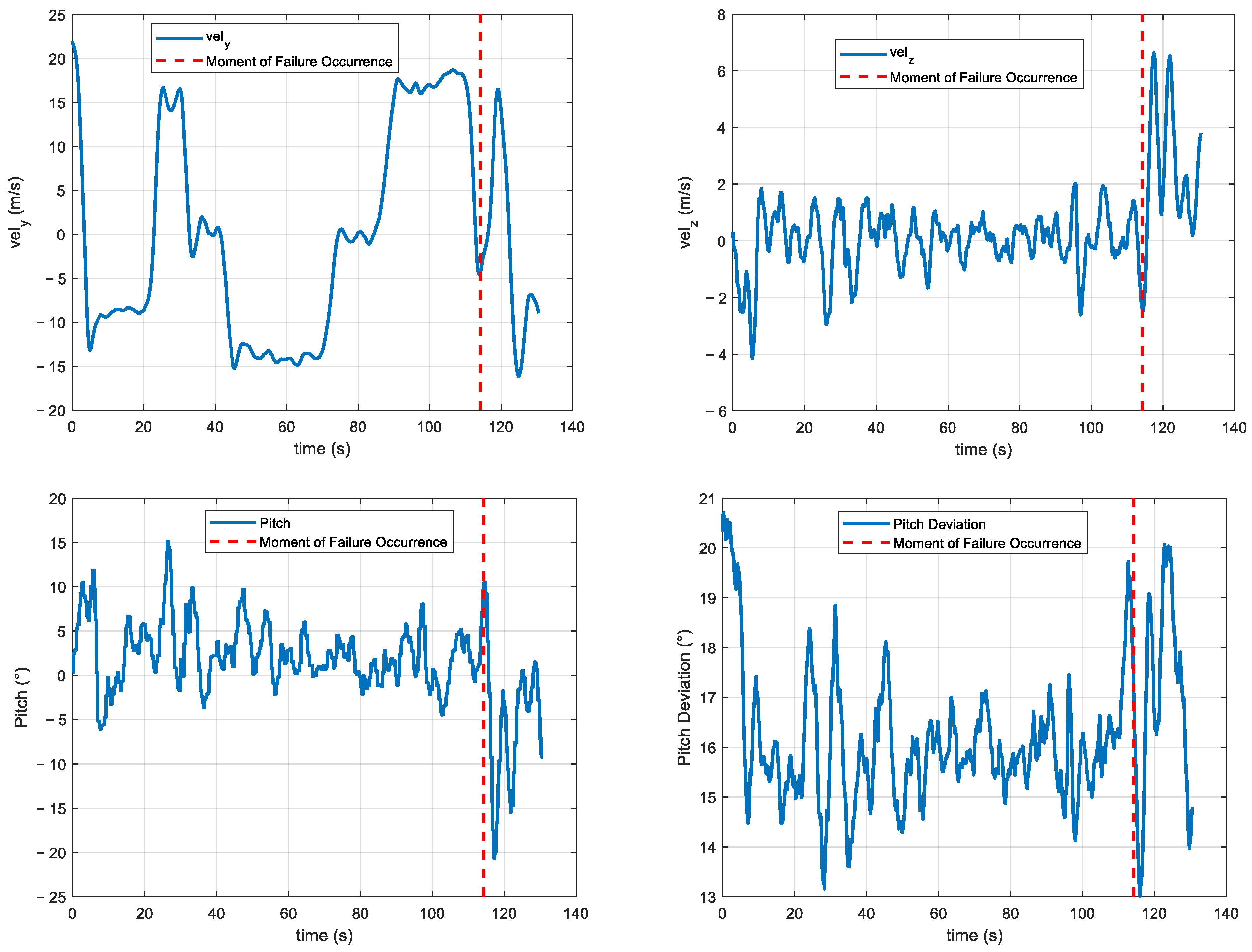
From Figure 4, it can be seen that, when the UAV’s engine completely failed, certain features exhibit significant changes after the failures, indicating their relevance to the faults. The velocity features ($V_x$, $V_y$, and $V_z$) show noticeable fluctuations, particularly after the red-dashed line, suggesting instability in the UAV’s speed along these axes following the engine failures. The pitch control (pitch and commands) also shows an increased difference between the actual and desired values after the failures, indicating that the pitch control is affected. Additionally, the airspeed exhibits significant changes, such as fluctuations or a decrease, typically due to the loss of engine power. In summary, the changes in velocity, roll, yaw, pitch, and airspeed can serve as important indicators for detecting UAV engine failure.

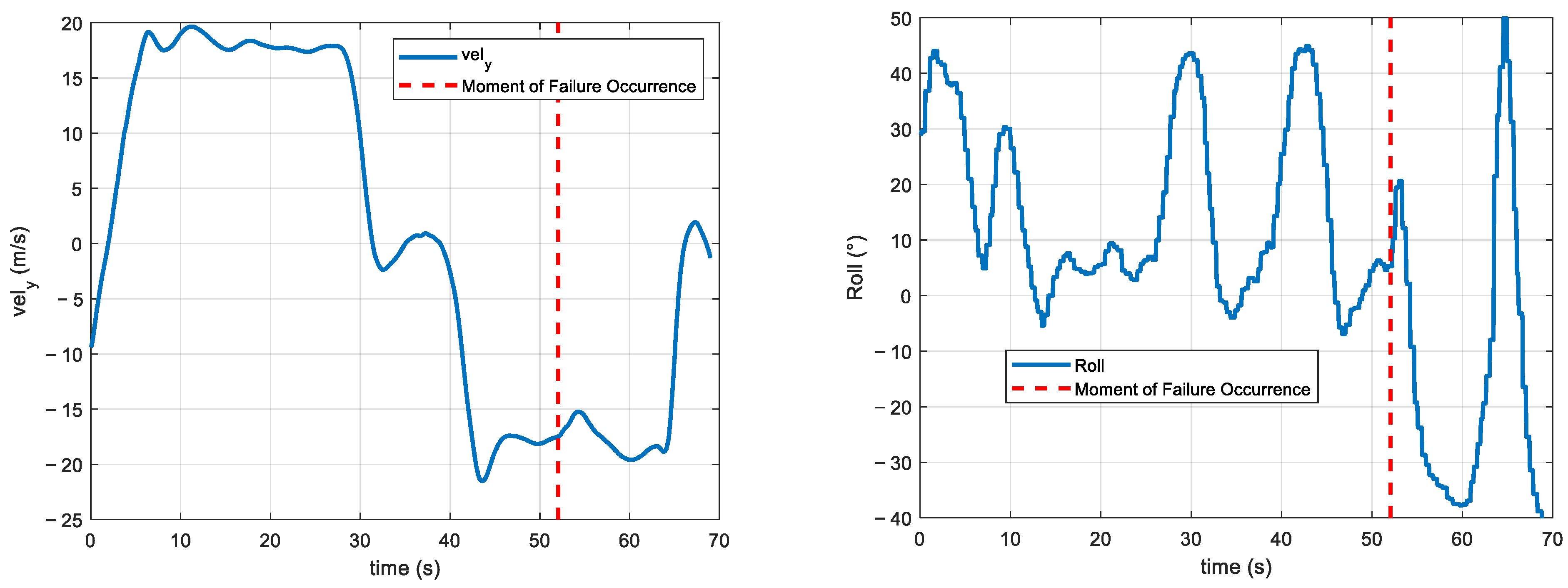
From Figure 5, it can be seen that, when the UAV’s rudder is stuck to the right, certain features exhibit significant changes after the failure. The acceleration features ($ac{c}_x$ and $ac{c}_y$) show noticeable fluctuations after the failure, particularly a significant increase in amplitude after the red-dashed line, indicating substantial changes in the acceleration characteristics in these directions following the rudder deviation. Although $ac{c}_z$ also shows some changes, they are less pronounced than those of $ac{c}_x$ and $ac{c}_y$. The velocity features ($V_x$ and $V_y$) display significant fluctuations after the failure, especially more pronounced changes in $V_y$, suggesting instability in the UAV’s speed following the rudder deviation, while the changes in $V_z$ are relatively smaller. The roll characteristics (roll and roll command) show an increased deviation between the actual and desired values after the failure, indicating instability in the roll control. Similarly, the yaw characteristics (yaw and yaw command) exhibit significant differences after the failure, with the actual values deviating more from the desired values, suggesting that the yaw control is affected. In summary, the acceleration features ($ac{c}_x$ and $ac{c}_y$), velocity features ($V_x$ and $V_y$), roll, and yaw show significant changes after the rudder deviation failure, indicating that these features are closely related to the failure and can serve as important references for anomaly detection and fault diagnosis.

Based on the analysis of the features associated with two different UAV failures, it was found that engine failure primarily affects the velocity, airspeed, and attitude control, while the rudder being stuck to the right significantly impacts the attitude angles, linear acceleration, velocity, and spatial position. Therefore, the features listed in Table 2 effectively reflect the changes in the UAV after a failure, and these significant variations can serve as key indicators for anomaly detection, providing a reliable basis for detection algorithms. Since multiple failure features may be simultaneously correlated and change when a failure occurs, exhibiting complex multi-dimensional dynamics, it is difficult to accurately detect and diagnose failures using a single feature or a fixed threshold. In the following sections, this study will use these failure features to conduct experiments on UAV anomaly detection algorithms.

5.2. Evaluation Metrics

This research employes five evaluation metrics—accuracy ($Acc$), $Precision$, $Recall$, $F1-score$, and $G-mean$—to demonstrate the effectiveness of the anomaly detection results. The calculation formulas for these evaluation metrics are shown in Equations (44)–(48), where $TP$ indicates the count of instances correctly classified as target data, $FN$ denotes the instances where target data are mistakenly identified as anomalies, $FP$ refers to the cases where anomalous data are wrongly classified as target data, and $TN$ signifies the instances where anomalous data are accurately classified as anomalies.

$$Acc={\displaystyle \frac{TP+TN}{TP+TN+FP+FN}}$$

(44)

$$Precision={\displaystyle \frac{TP}{TP+FP}}$$

(45)

$$Recall={\displaystyle \frac{TP}{TP+FN}}$$

(46)

$$F1-score={\displaystyle \frac{2\times Precision\times Recall}{Precision+Recall}}$$

(47)

$$G-mean=\sqrt{Recall\times {\displaystyle \frac{TN}{\left(TN+FP\right)}}}$$

(48)

5.3. Experimental Analysis of Sliding Window Parameters for Anomaly Detection

The flight data reconstruction process utilizes a sliding window approach to segment the time series data, effectively capturing the temporal correlations within the data. The reconstructed flight data are closely related to the sliding window length and stride. To analyze the impact of these two parameters on the anomaly detection accuracy, we designed two experiments:

• Experiment 1: The stride is set to 1, and the sliding window length is varied to observe its effect on the accuracy of the anomaly detection algorithm.
• Experiment 2: The sliding window length is set to 25, and different strides are tested to examine their impact on the accuracy of the anomaly detection algorithm.

The goal of these experiments is to determine how the choice of the sliding window length and stride affects the detection accuracy of the model under a given dataset and anomaly detection model. The anomaly detection algorithm uses an autoencoder, detecting anomalies by comparing the residuals between the original data and the reconstructed data against a threshold, which is chosen based on the 3σ rule.

(1)

Impact of Different Sliding Window Lengths on Anomaly Detection Accuracy

The sliding window length is chosen from a predefined set of values, and for each selected length, the data are reconstructed into a multi-dimensional time series input. A new dataset version is generated for each sliding window length, and the same anomaly detection algorithm is used to train and test on each reconstructed dataset version.

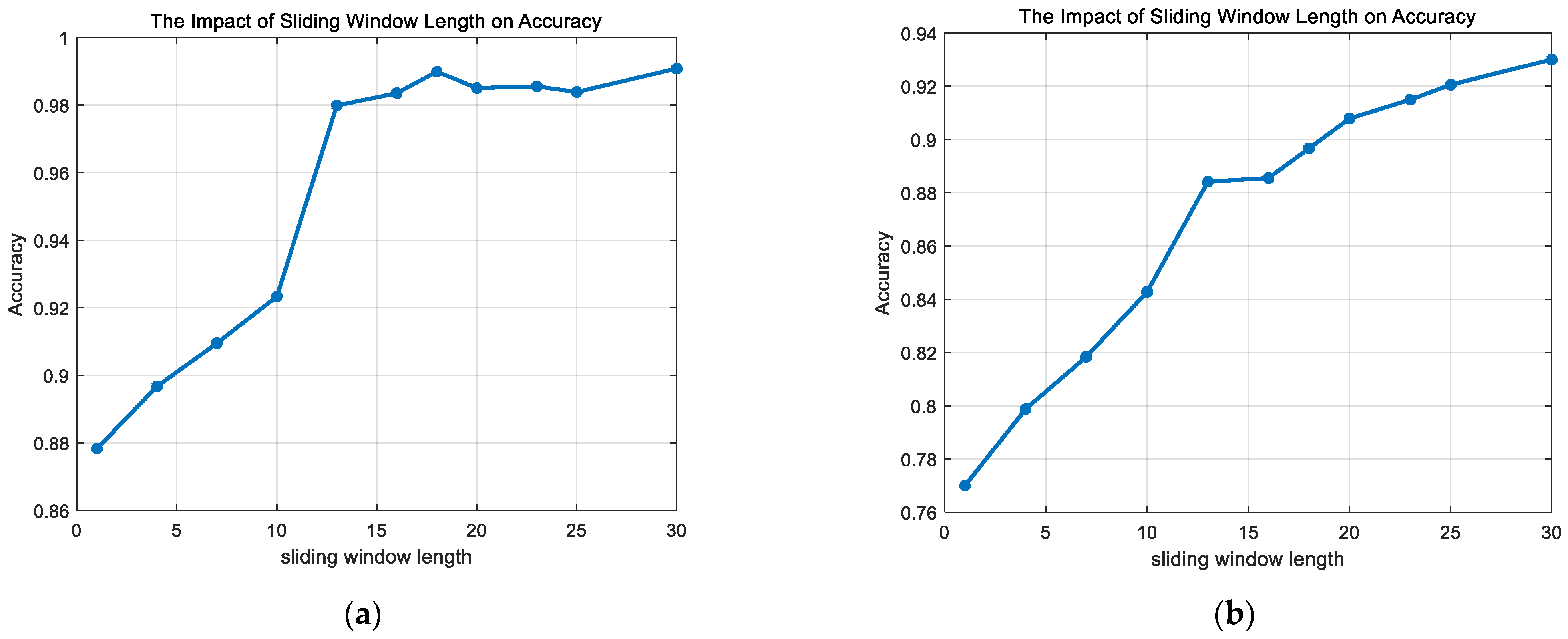
As shown in Figure 6, the accuracy of the anomaly detection algorithm improves as the sliding window length increases. When the sliding window length exceeds 20, further increasing the length has little to no effect on the accuracy. A larger sliding window length means that each window covers more data points, allowing the model to capture data features over a longer time range, which helps the model to better understand and utilize the long-term trends or patterns in the time series. However, a larger window also increases the number of data points within each window, significantly raising the computation time and resource consumption. Considering these factors, the sliding window length is set to 25 in this study.

(2)

Impact of Different Strides on Anomaly Detection Accuracy

The stride is chosen from a predefined set of values. Based on a fixed sliding window length and different strides, the data are reconstructed into a multi-dimensional time series input. Each stride generates a new dataset version, and the same anomaly detection algorithm is used to train and test on each reconstructed dataset version.

As shown in Figure 7, the accuracy of the anomaly detection algorithm gradually decreases as the stride increases. A larger stride means that the sliding window moves a greater distance in the data sequence with each step, resulting in fewer sliding windows and, consequently, fewer data samples for model training. While this can speed up the training and prediction process, the reduced number of samples may result in the insufficient learning of the data by the model, thereby decreasing the accuracy of the anomaly detection. Considering these factors, the stride for the sliding window is set to 1 in this study.

Based on the experimental analysis, in this study, the sliding window length is set to 25 with a stride of 1, and the flight feature data are reconstructed using the sliding window method. This process yields the training and validation datasets.

5.4. CAE Model Training

For the CAE model parameter settings, the starting learning rate was set to 0.001. The optimizer utilized was Adam, and the mean squared error (MSE) function was used for reconstruction loss. The encoding and decoding layers of the CAE model each consisted of two 1DCNNs. The parameter settings for the convolutional layers are detailed in

Table 3. Convolutional layer parameters of experiment.

Component	Lay Type	Lay Number	Number of Filters	Filter Lengths	Stride
Encoder	Convolutional Layer	1	32	10	2
Encoder	Convolutional Layer	2	16	10	2
Decoder	Deconvolutional Layer	1	16	10	2
Decoder	Deconvolutional Layer	2	32	10	2

.

The figure below illustrates the reconstructed residuals from the CAE model’s dataset.

In Figure 8, it can be seen that for the rudder anomalies, there is a significant difference between the normal data and the anomalous data reconstructed by the CAE. However, for the “rudder and aileron at zero” anomaly, a small portion of the reconstruction error values for the anomalous data are close to those of the normal data. For the right aileron anomaly, a larger portion of the reconstruction error values for the anomalous data are close to those of the normal data, making it difficult to determine a threshold that distinguishes between the normal and anomalous data.

5.5. Anomaly Detection

To demonstrate the effectiveness of the proposed algorithm, this study selected several anomaly detection methods for comparative experiments. Here is an overview of the methods chosen:

(1)

SVDD [36]: As a one-class classification method, SVDD uses a kernel function to map the input data onto a high-dimensional space and find the optimal hyperplane with which to separate the normal and abnormal samples. It performs well in anomaly detection, particularly with high-dimensional data, making it effective for evaluating the performance of our algorithm.

(2)

LSTM [25]: LSTM is a deep learning sequence modeling method that excels at capturing long-term dependencies. It can predict future states by learning the patterns of the historical data and detecting anomalies. Its strong ability to handle time series data makes it an ideal benchmark model for anomaly detection in UAV data.

(3)

LSTM-AE [32]: LSTM-AE combines the sequence modeling capabilities of LSTM with the reconstruction abilities of an autoencoder, enabling it to better learn the temporal features of normal UAV flight states and quickly detect abnormal patterns. It has been widely applied in UAV anomaly detection, making it an important comparative model.

(4)

Autoencoder [30]: As a classic unsupervised learning model, the autoencoder performs dimensionality reduction and reconstruction to learn the representation and features of normal data. It achieves anomaly detection by comparing the reconstruction residuals with a threshold. Its effectiveness across various data types (including images and time series) makes it a representative benchmark model.

Both SVDD and the proposed method use the Gaussian kernel function. The parameter $c$ for regularization was selected from $\left\{0.1,0.5,1,5,10,20\right\}$, and the Gaussian kernel parameter $\sigma$ was selected from $\left\{2^{-5}s,2^{-4}s,\dots ,2^{4}s,2^{5}s\right\}$, where $s$ denotes the mean Euclidean distance across all training instances [41]. The iteration numbers for the AE, LSTM, and LSTM-AE were set to 400, using the Adam optimizer and the mean squared error (MSE) as the loss function. The learning rate for the AE was 0.001, while the learning rate for the LSTM and LSTM-AE was 0.0008. The rest of the experimental environment was consistent with that of the previous experiment. For anomaly detection, the AE, LSTM, and LSTM-AE detected anomalies by evaluating the residuals between the original dataset and the observed data against a specified threshold. To ensure fairness in the experiments, the 3σ principle was used to select the threshold for the comparative experiments. The SVDD and CAE-L0/1-SVDD distinguished between the normal and anomalous samples using a hypersphere.

The experimental results of the ALFA dataset are reported in

Table 4. Results of anomaly detection using various methods based on ALFA dataset.

Type of Anomaly	Method	Evaluation Metrics
		Acc	Precision	Recall	F1-Score	G-mean
Engine failure	SVDD	0.9021	0.8794	0.9863	0.9298	0.8546
	LSTM	0.9862	0.9843	0.9949	0.9896	0.9871
	AE	0.9879	1	0.9181	0.9908	0.9909
	LSTM-AE	0.9919	0.9906	0.9888	0.9897	0.9913
	Our	0.9926	0.9931	0.9969	0.9950	0.9885
Rudder stuck to the left	SVDD	0.9786	0.9910	0.9800	0.9855	0.9773
	LSTM	0.9891	1	0.9842	0.9920	0.9921
	AE	0.9836	1	0.9597	0.9795	0.9797
	LSTM-AE	0.9674	1	0.9526	0.9757	0.9760
	Our	0.9966	1	0.9955	0.9977	0.9977
Rudder stuck to the right	SVDD	0.9554	0.9624	0.9690	0.9657	0.9657
	LSTM	0.9791	1	0.9596	0.9794	0.9796
	AE	0.9903	1	0.9625	0.9809	0.9811
	LSTM-AE	0.9971	1	0.9888	0.9944	0.9944
	Our	0.9985	1	0.9975	0.9987	0.9987
Elevator stuck at zero	SVDD	0.8620	0.9026	0.9816	0.9405	0.8578
	LSTM	0.9525	0.9505	0.9851	0.9675	0.9253
	AE	0.9530	0.9618	0.9733	0.9675	0.9366
	LSTM-AE	0.9765	1	0.9673	0.9834	0.9835
	Our	0.9912	0.9955	0.9933	0.9944	0.9885
Left aileron stuck at zero	SVDD	0.6129	0.4081	0.9432	0.6796	0.5697
	LSTM	0.5414	0.1936	0.9912	0.3239	0.6936
	AE	0.5947	0.4006	0.9840	0.5994	0.6646
	LSTM-AE	0.6665	0.4482	0.9771	0.6145	0.7334
	Our	0.9549	0.9051	0.9727	0.9377	0.9590
Right aileron stuck at zero	SVDD	0.6550	0.5946	0.9720	0.7378	0.7378
	LSTM	0.5625	0.5362	0.9817	0.6936	0.3652
	AE	0.6320	0.5796	0.9845	0.7297	0.5187
	LSTM-AE	0.7537	0.6729	0.9901	0.8012	0.7149
	Our	0.9582	0.9653	0.9641	0.9647	0.9568
Both ailerons stuck at zero	SVDD	0.8986	0.9044	0.9126	0.9083	0.8865
	LSTM	0.9822	1	0.9506	0.9747	0.9747
	AE	0.9896	1	0.9712	0.9854	0.9855
	LSTM-AE	0.9962	0.9938	0.9817	0.9877	0.9902
	Our	0.9982	1	0.9959	0.9979	0.9979
Rudder and aileron at zero	SVDD	0.8597	0.8110	0.9794	0.8873	0.8310
	LSTM	0.9301	0.9	0.9873	0.9416	0.9183
	AE	0.9236	0.8163	0.9653	0.8847	0.9350
	LSTM-AE	0.9466	0.9337	0.9758	0.9543	0.9412
	Our	0.9879	0.9851	0.9965	0.9908	0.9839

. The best results are highlighted in bold and underline in the table footer. In Table 4, it can be observed that the SVDD method’s performance in anomaly detection was less effective compared to the approaches utilizing LSTM, AE, and LSTM-AE, as well as the CAE-L0/1-SVDD. The SVDD method had a high rate of false alarms, indicating that it unreasonably neglected the complex spatial correlations among the flight data. In contrast, the LSTM, AE, LSTM-AE, and CAE-L0/1-SVDD methods performed well in detecting the four types of anomalies: “rudder stuck to the left”, “rudder stuck to the right”, “ailerons stuck at zero”, and “engine failure”. According to the reconstruction residuals from the dataset, the reconstruction error values for these four types of anomalies showed significant differences compared with the normal data, making it possible to effectively detect anomalies by appropriately selecting a threshold. However, for the two anomalies “rudder and aileron stuck at zero” and “elevator stuck at zero”, some of the reconstruction error values of the anomalous data were close to those of the normal data, making it easy to misjudge when using a fixed threshold. Therefore, in these cases, the accuracy of the LSTM, AE, and LSTM-AE methods was lower than that of the CAE-L0/1-SVDD. For the anomalies “left aileron stuck at zero” and “right aileron stuck at zero”, a significant portion of the anomalous data’s reconstruction error for the anomalous data were similar to those of the normal data, increasing the risk of misclassification when a fixed threshold is applied. In this situation, the accuracy of the AE, LSTM, and LSTM-AE methods was significantly lower than that of the CAE-L0/1-SVDD. The experiments with real data show that the proposed CAE model comprehensively accounted for the spatiotemporal correlations in the flight data and efficiently extracted the relevant features. When the reconstruction and prediction errors of the anomalous data closely matched those of the normal data, the L0/1-SVDD approach was effective in detecting anomalies.

From Figure 9, it can be observed that the area under the curve (AUC) values of the SVDD method are lower than those of the LSTM, AE, LSTM-AE, and CAE-L0/1-SVDD methods across all the datasets. For some datasets, the AUC values of the SVDD range from 0.62 to 0.98, indicating significant performance fluctuations and limited applicability across different types of datasets. The AE and LSTM methods perform well on most of the datasets, with AUC values typically close to 1.00, but their performance drops on the “left aileron stuck at zero” and “right aileron stuck at zero” datasets, with their AUC values falling to 0.63 or 0.82, respectively. The LSTM-AE method also shows excellent performance, with AUC values close to or reaching 1.00 for all the datasets except the “right aileron stuck at zero” dataset, demonstrating strong anomaly detection capabilities. The CAE-L0/1-SVDD method achieves perfect AUC values (1.00) across all the datasets, showcasing its superior performance, stability, and robustness in anomaly detection tasks, making it the best-performing method among those tested.

6. Conclusions

Anomaly detection based on UAV flight data is one of the key methods for enhancing UAV flight safety. This study proposed a framework combining CAE and L0/1-SVDD to enhance UAV anomaly detection performance. First, a CAE model based on a 1DCNN and an AE was established as an alternative to existing methods. This model combined the feature extraction capabilities of the 1DCNN with the reconstruction capabilities of the AE to extract the spatiotemporal features from the data. To address the issue of adaptive anomaly detection thresholds, it was noted that the difference between the reconstructed values and the actual values in the CAE model may contain outliers, and that the traditional SVDD algorithm was highly sensitive to noise and outliers in the training data. Therefore, this study proposed an SVDD method utilizing the 0/1 loss function, replacing the traditional hinge loss function in SVDD with a 0/1 loss function, and solving this nonlinear model using the Bregman ADMM algorithm. Then, the L0/1-SVDD threshold determination module was trained using the residuals, allowing for a more accurate threshold determination and further improving the anomaly detection performance. The experimental results indicate that the proposed anomaly detection algorithm outperforms currently popular methods, such as the SVDD, autoencoder, LSTM, and LSTM-AE, in terms of accuracy, precision, recall, F1-score, and G-mean. Although this research makes new contributions to the technical field, there are still some limitations that warrant further investigation. First, the current deep learning feature extraction method is primarily based on historical healthy data in real time; future research could consider incorporating a small number of anomalous data in the model training. Second, the anomaly detection method proposed in this study, which combines CAE and L0/1-SVDD, increases the model’s parameters. Future work may need to explore the introduction of intelligent optimization algorithms to determine the model parameters. Additionally, incorporating the 0/1 loss function into the L0/1-SVDD framework creates a non-convex optimization challenge, significantly raising the computational complexity and complicating the search for a globally optimal solution. When handling large-scale datasets, the training time can substantially increase. Therefore, future research could explore using a distributed computing framework to speed up the L0/1-SVDD model’s training process.

References

1. Cho, J.; Kim, C.; Lim, K.J.; Kim, J.; Ji, B.; Yeon, J. Web-based agricultural infrastructure digital twin system integrated with GIS and BIM concepts. Comput. Electron. Agric. 2023, 215, 108441. [Google Scholar] [CrossRef]
2. Alkadi, R.; Shoufan, A. Unmanned Aerial Vehicles Traffic Management Solution Using Crowd-Sensing and Blockchain. IEEE Trans. Netw. Serv. Manag. 2023, 20, 201–215. [Google Scholar] [CrossRef]
3. Mohsan, S.A.H.; Othman, N.Q.H.; Li, Y.; Alsharif, M.H.; Khan, M.A. Unmanned aerial vehicles (UAVs): Practical aspects, applications, open challenges, security issues, and future trends. Intell. Serv. Robot. 2023, 16, 109–137. [Google Scholar] [CrossRef]
4. Radoglou-Grammatikis, P.; Sarigiannidis, P.; Lagkas, T.; Moscholios, I. A compilation of UAV applications for precision agriculture. Comput. Netw. 2020, 172, 107148. [Google Scholar] [CrossRef]
5. Maimaitijiang, M.; Sagan, V.; Sidike, P.; Hartling, S.; Esposito, F.; Fritschi, F.B. Soybean yield prediction from UAV using multimodal data fusion and deep learning. Remote Sens. Environ. 2020, 237, 111599. [Google Scholar] [CrossRef]
6. Puchalski, R.; Giernacki, W. UAV fault detection methods state-of-the-art. Drones 2022, 6, 330. [Google Scholar] [CrossRef]
7. Yang, L.; Li, S.; Li, C.; Zhang, A.; Zhang, X. A survey of unmanned aerial vehicle flight data anomaly detection: Technologies, applications, and future directions. Sci. China Technol. Sci. 2023, 66, 901–919. [Google Scholar] [CrossRef]
8. Shao, G.; Ma, Y.; Malekian, R.; Yan, X.; Li, Z. A novel cooperative platform design for coupled USV-UAV systems. IEEE Trans. Ind. Inf. 2019, 15, 4913–4922. [Google Scholar] [CrossRef]
9. Abbaspour, A.; Aboutalebi, P.; Yen, K.K.; Sargolzaei, A. Neural adaptive observer-based sensor and actuator fault detection in nonlinear systems:Application in UAV. ISA Trans. 2017, 67, 317–329. [Google Scholar] [CrossRef] [PubMed]
10. Guo, D.; Zhong, M.; Zhou, D. Multisensor data-fusion-based approach to airspeed measurement fault detection for unmanned aerial vehicles. IEEE Trans. Instrum. Meas. 2017, 67, 317–327. [Google Scholar] [CrossRef]
11. Rosa, R.L.; Schwartz, G.M.; Ruggiero, W.V.; Rodríguez, D.Z. A Knowledge-Based Recommendation System That Includes Sentiment Analysis and Deep Learning. IEEE Trans. Ind. Inform. 2019, 15, 2124–2135. [Google Scholar] [CrossRef]
12. Erkan, C.O. Vibration data-driven anomaly detection in UAVs: A deep learning approach. Eng. Sci. Technol. Int. J. 2024, 54, 101702. [Google Scholar] [CrossRef]
13. Zhang, Y.; Meratnia, N.; Havinga, P. Outlier detection techniques for wireless sensor networks: A survey. IEEE Commun. Surv. Tutor. 2010, 12, 159–170. [Google Scholar] [CrossRef]
14. Rassam, M.A.; Zainal, A.; Maarof, M.A. Advancements of data anomaly detection research in wireless sensor networks: A survey and open issues. Sensors 2013, 13, 10087–10122. [Google Scholar] [CrossRef]
15. Alam, S.; Sonbhadra, S.K.; Agarwal, S.; Nagabhushan, P. One-class support vector classifiers: A survey. Knowl.-Based Syst. 2020, 196, 105754. [Google Scholar] [CrossRef]
16. Wang, H.; Shao, Y.; Zhou, S.; Zhang, C.; Xiu, N. Support Vector Machine Classifier via L0/1 Soft-Margin Loss. IEEE Trans. Pattern Anal. Mach. Intell. 2022, 44, 7253–7265. [Google Scholar] [CrossRef]
17. Lin, R.; Yao, Y.; Liu, Y. Kernel support vector machine classifiers with ℓ0-norm hinge loss. Neurocomputing 2024, 589, 127669. [Google Scholar] [CrossRef]
18. Liu, Y.; Ding, W. A KNNS based anomaly detection method applied for UAV flight data stream. In Proceedings of the Prognostics and System Health Management Conference (PHM), Beijing, China, 21–23 October 2015; pp. 1–8. [Google Scholar]
19. Pan, D.; Nie, L.; Kang, W.; Song, Z. UAV anomaly detection using active learning and improved S3 VM model. In Proceedings of the International Conference on Sensing, Measurement & Data Analytics in the Era of Artificial Intelligence (ICSMD), Xi’an, China, 15–17 October 2020; pp. 253–258. [Google Scholar]
20. Song, L.K.; Li, X.Q.; Zhu, S.P.; Choy, Y.S. Cascade ensemble learning for multi-level reliability evaluation. Aerosp. Sci. Technol. 2024, 148, 109101. [Google Scholar] [CrossRef]
21. Whelan, J.; Almehmadi, A.; El-Khatib, K. Artificial intelligence for intrusion detection systems in unmanned aerial vehicles. Comput. Electr. Eng. 2022, 99, 107784. [Google Scholar] [CrossRef]
22. Al-Haddad, L.A.; Jaber, A.A. An intelligent fault diagnosis approach for multirotor UAVs based on deep neural network of multi-resolution transform features. Drones 2023, 7, 82. [Google Scholar] [CrossRef]
23. Al-lQubaydhi, N.; Alenezi, A.; Alanazi, T.; Senyor, A.; Alanezi, N.; Alotaibi, B.; Alotaibi, M.; Razaque, A.; Hariri, S. Deep learning for unmanned aerial vehicles detection: A review. Comput. Sci. Rev. 2024, 51, 100614. [Google Scholar] [CrossRef]
24. Ahmad, M.W.; Akram, M.U.; Ahmad, R.; Hameed, K.; Hassan, A. Intelligent framework for automated failure prediction, detection, and classification of mission critical autonomous flights. ISA Trans. 2022, 129 Pt A, 355–371. [Google Scholar] [CrossRef]
25. Choi, K.; Yi, J.; Park, C.; Yoon, S. Deep learning for anomaly detection in time-series data: Review, analysis, and guidelines. IEEE Access 2021, 9, 120043–120065. [Google Scholar] [CrossRef]
26. Pang, G.; Shen, C.; Cao, L.; Hengel, A.V.D. Deep learning for anomaly detection: A review. ACM Comput. Surv. 2021, 54, 1–38. [Google Scholar] [CrossRef]
27. Zhong, J.; Zhang, Y.; Wang, J.; Luo, C.; Miao, Q. Unmanned Aerial Vehicle Flight Data Anomaly Detection and Recovery Prediction Based on Spatio-Temporal Correlation. IEEE Trans. Reliab. 2022, 71, 457–468. [Google Scholar] [CrossRef]
28. Chang, X.; Rong, L.; Chen, K.; Fu, W. LSTM-based output-constrained adaptive fault-tolerant control for fixed-wing UAV with high dynamic disturbances and actuator faults. Math. Probl. Eng. 2021, 2021, 8882312. [Google Scholar] [CrossRef]
29. Wang, B.; Liu, D.; Peng, Y.; Peng, X. Multivariate Regression-Based Fault Detection and Recovery of UAV Flight Data. IEEE Trans. Instrum. Meas. 2020, 69, 3527–3537. [Google Scholar] [CrossRef]
30. Wang, B.; Peng, X.; Jiang, M.; Liu, D. Real-Time Fault Detection for UAV Based on Model Acceleration Engine. IEEE Trans. Instrum. Meas. 2020, 69, 9505–9516. [Google Scholar] [CrossRef]
31. Guo, K.; Wang, N.; Liu, D.; Peng, X. Uncertainty-Aware LSTM Based Dynamic Flight Fault Detection for UAV Actuator. IEEE Trans. Instrum. Meas. 2023, 72, 3502113. [Google Scholar] [CrossRef]
32. Park, K.H.; Park, E.; Kim, H.K. Unsupervised fault detection on unmanned aerial vehicles: Encoding and thresholding approach. Sensors 2021, 21, 2208. [Google Scholar] [CrossRef]
33. Jiang, G.; Nan, P.; Zhang, J.; Li, Y.; Li, X. Robust Spatial-Temporal Autoencoder for Unsupervised Anomaly Detection of Unmanned Aerial Vehicle with Flight Data. IEEE Trans. Instrum. Meas. 2024, 73, 3526014. [Google Scholar] [CrossRef]
34. Bae, G.; Joe, I. UAV anomaly detection with distributed artificial intelligence based on LSTM-AE and AE. In Advanced Multimedia and Ubiquitous Engineering; Park, J., Yang, L., Jeong, Y.S., Hao, F., Eds.; Lecture Notes in Electrical Engineering; Springer: Singapore, 2019; Volume 590. [Google Scholar]
35. Yang, L.; Li, S.; Zhu, C.; Zhang, A.; Liao, Z. Spatio-temporal correlation-based multiple regression for anomaly detection and recovery of unmanned aerial vehicle flight data. Adv. Eng. Inform. 2024, 60, 102440. [Google Scholar] [CrossRef]
36. Schmidhuber, J. Deep learning in neural networks: An overview. Neural Netw. 2015, 61, 85–117. [Google Scholar] [CrossRef] [PubMed]
37. Tax, D.M.J.; Duin, R.P.W. Support vector data description. Mach. Learn. 2004, 54, 45–66. [Google Scholar] [CrossRef]
38. Scholkopf, B.; Herbrich, R.; Smola, A.J. A generalized representer theorem. In Proceedings of the 14th Annual Conference on Computational Learning Theory, Amsterdam, The Netherlands, 16–19 July 2001; pp. 416–426. [Google Scholar] [CrossRef]
39. Wang, H.J.; Shao, Y.H.; Xiu, N.H. Proximal operator and optimality conditions for ramp loss SVM. Optim. Lett. 2022, 16, 999–1014. [Google Scholar] [CrossRef]
40. Keipour, A.; Mousaei, M.; Scherer, S. ALFA: A dataset for UAV fault and anomaly detection. Int. J. Robot. Res. 2021, 40, 515–520. [Google Scholar] [CrossRef]
41. Hu, W.; Hu, T.; Wei, Y.; Lou, J.; Wang, S. Global Plus Local Jointly Regularized Support Vector Data Description for Novelty Detection. IEEE Trans. Neural Netw. Learn. Syst. 2023, 34, 6602–6614. [Google Scholar] [CrossRef] [PubMed]
Figure 1. Autoencoder.
Drones 08 00534 g001
Figure 2. The overall framework for UAV anomaly detection.
Drones 08 00534 g002
Figure 3. Diagram of the architecture of the CAE model.
Drones 08 00534 g003
Figure 4. Feature change curves during UAV engine failure.
Drones 08 00534 g004
Figure 5. Feature change curves when the UAV’s rudder is stuck to the right.
Drones 08 00534 g005aDrones 08 00534 g005b
Figure 6. The impact of different sliding window lengths on the anomaly detection accuracy: (a) engine failure; (b) rudder and aileron at zero.
Drones 08 00534 g006
Figure 7. Impact of different strides on anomaly detection accuracy: (a) engine failure; (b) rudder and aileron at zero.
Drones 08 00534 g007
Figure 8. Residuals of the reconstructed data for different types of anomalies: (a) rudder and aileron at zero; (b) rudder stuck to the left; (c) rudder stuck to the right; and (d) left aileron stuck at zero.
Drones 08 00534 g008
Figure 9. ROC curves for different anomaly detection methods: (a) engine failure; (b) rudder stuck to the left; (c) rudder stuck to the right; (d) elevator stuck at zero; (e) left aileron stuck at zero; (f) right aileron stuck at zero; (g) both ailerons stuck at zero; (h) rudder and aileron at zero.
Drones 08 00534 g009aDrones 08 00534 g009b