1. Introduction
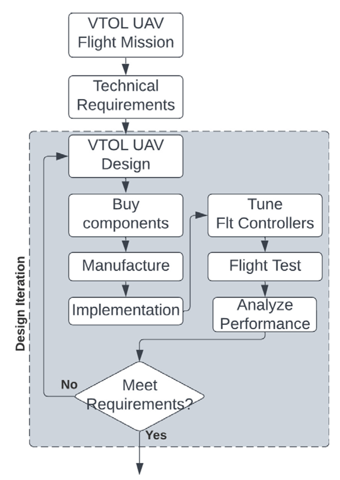
UAV designs vary due to mission requirement and system performance. As the scale of the UAV increases, the design modification and fabrication processes are added to ensure a successful outcome, as referred to in
Figure 1. The building costs and manpower for the development of tasks in the yellow blocks increase drastically. It is known that each change from the preliminary design may cause significant reconsideration and add a tedious workload to the whole project. For a full-scale rotorcraft UAV, its cost is about USD 75 k/hour for the flight test and 35% of that cost falls within the flight control [
1]. The same scale of development cost is also applied to the UAV development program. Simulation with minor real flight tests can be useful to speed up the development process toward an accurate result [
1]. Under the aegis of such a concept, this approach to developing larger-scale UAVs or urban air mobility (UAM) vehicles will not be a practical investment from a business standpoint. There is quite a demand to establish a method to predict the design performance of these vehicles with at least 80% accuracy without building the real vehicle in the preliminary study and design. This leads to a significant reduction in time and cost for design iterations.
Today, flight simulators are quite mature in terms of flight dynamics analysis, the internal physics engine, and visualization. Using a flight simulator leverages thousands of hours for developers to evolve complex physical models, so that the flight simulator can be more reliable and have higher accuracy [
2]. Thanks to the establishment and sophistication of flight simulators in the past decade, more and more commercial and military pilots are trained using flight simulators [
3]. A detailed comparison of the commercial and open-source PC-based flight simulators applied from small UAVs to general-category aircrafts was undertaken by Dahlstrom et al. in [
4,
5]. They concluded that it is not worth developing a flight simulator from scratch. These studies by Dahlstrom and Alexander et al. [
4,
5] analyzed the quality of the flight simulators based on four criteria, including physical environment fidelity, functional fidelity, ease of development, and cost. The top five high-fidelity flight simulators from Dahlstrom et al. [
4] are shown in
Table 1.
Both X-Plane and Unity have high physical and functional fidelity. However, X-Plane has a lower cost and is easier to use. It is also important that FAA has certified X-Plane as a training simulator to run on certain hardware configurations. It results in high fidelity in its physical flight model. Moreover, there are many studies that use Matlab/Simulink (R2021b) in conjunction with X-Plane on the same PC (Windows OS) to develop and validate the flight controller, either in Software in the Loop (SIL) or Hardware in the Loop (HIL). With the advantages of a seamless PC-based (Windows OS) flight simulator setup (with X-Plane and Matlab/Simulink), the control signal from the pilot is sent to the flight simulator precisely, with minimum latency, and the same thing occurs for the UAV model’s flight data from the X-Plane in reverse. Furthermore, the flight test data could be analyzed directly using Matlab instead of firstly being copied from Linux (Ubuntu22) to Windows 10. Moreover, the latency, error, and complexity of passing the flight data between software in different operating systems could be avoided. These technical problems in passing data between OSs are very hard to detect, quantify, and verify whether it is a control problem or a communication problem in case the vehicle does not perform as expected. With the seamless PC-based flight simulator setup, not only are the time and cost to develop and test the flight controller reduced dramatically, but the pilot can directly fly the air vehicle in X-Plane and offer their comments immediately at each revision of the flight controller. This makes the design iteration much shorter and cheaper than the traditional design iteration shown in
Figure 1. As a result, X-Plane is chosen for the flight simulator in this study.
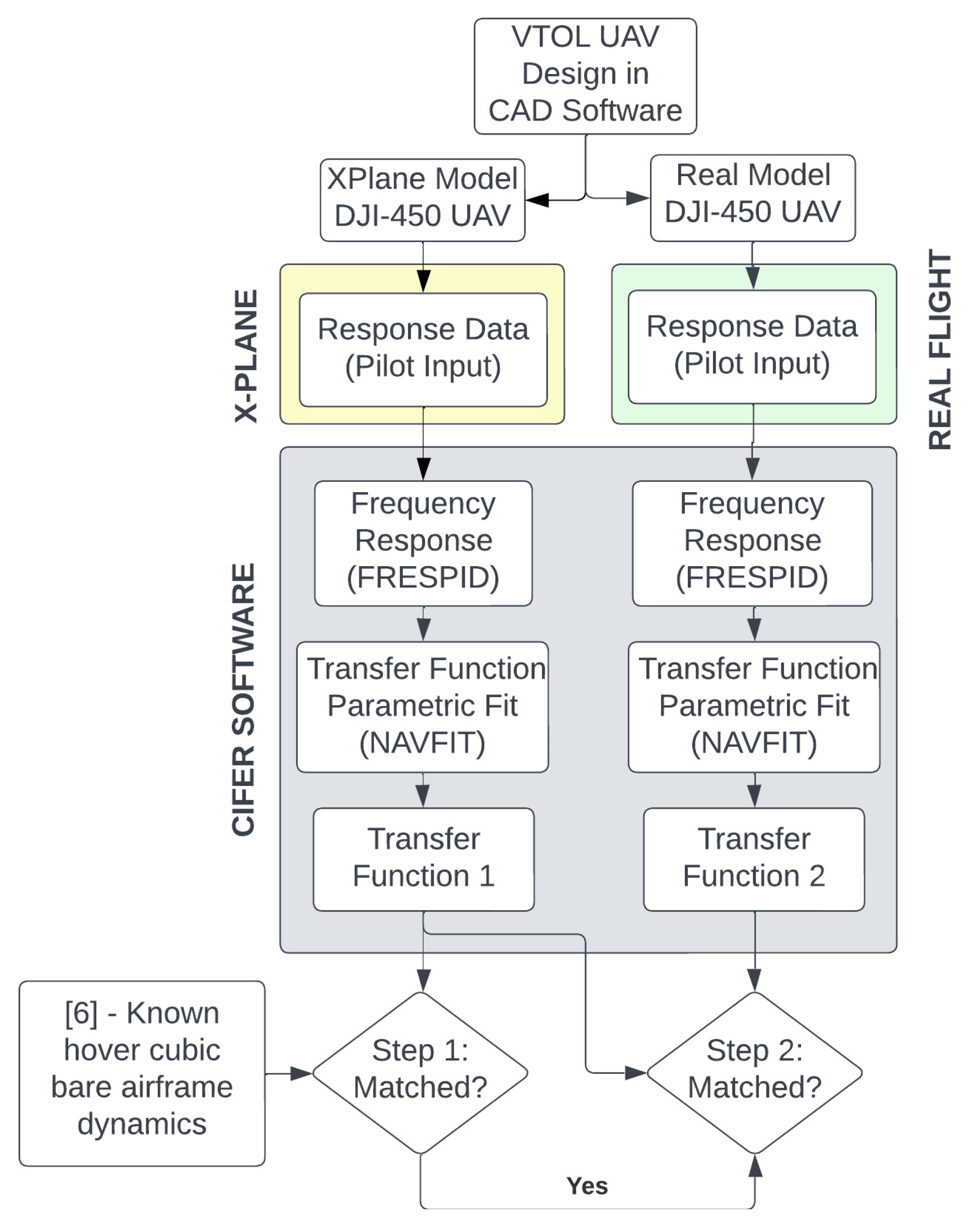
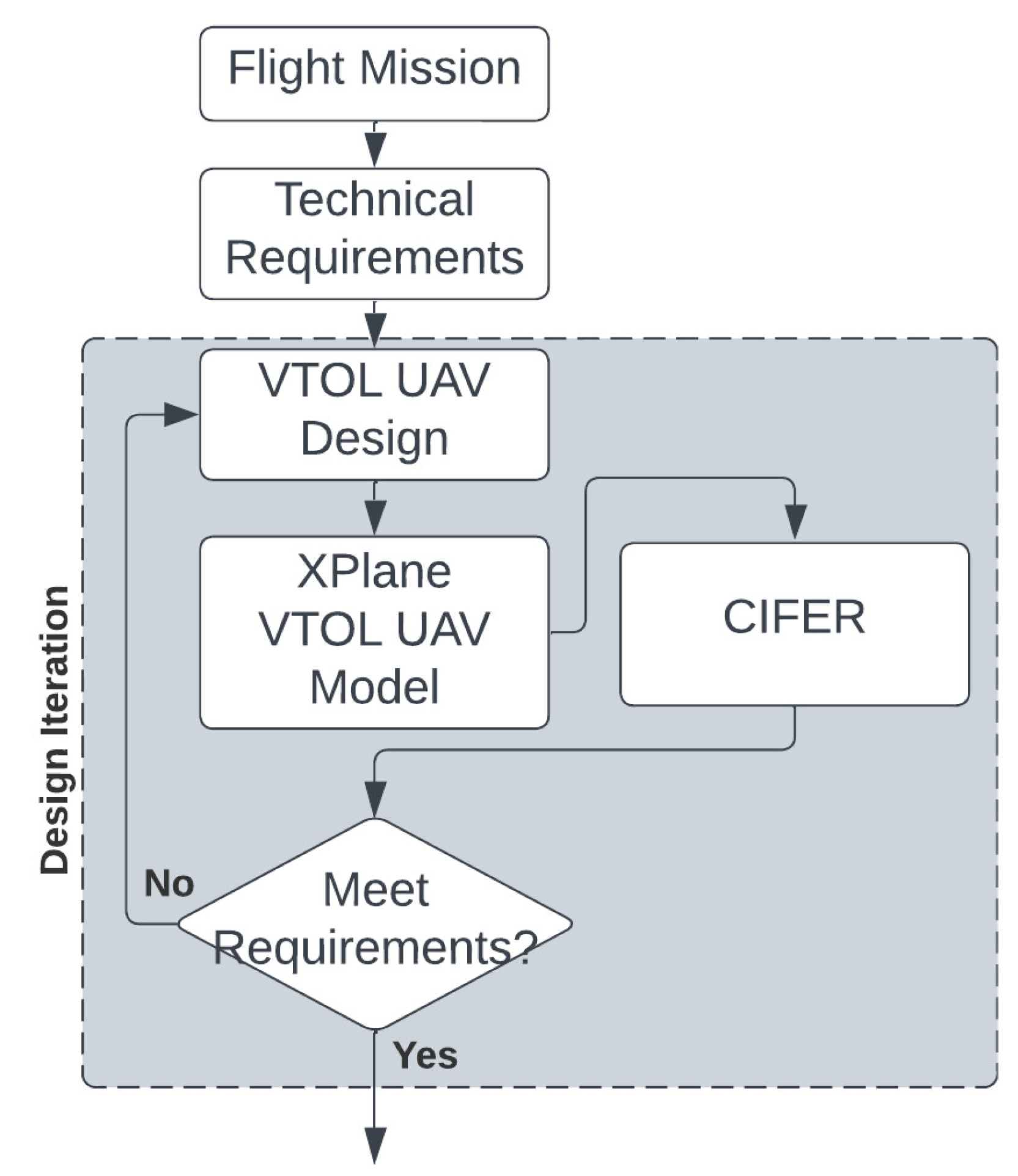
This paper proposes a new design process, as shown in
Figure 2. The proposed process predicts high accuracy for the quadrotor UAV flight dynamics at hover state without building the quadrotor UAV in the real world. In addition, guidance for building high-fidelity models in X-Plane is presented. There are two main steps to achieve this goal: validate the X-Plane dynamics engine qualitatively (step 1) and quantitatively (step 2).
X-Plane uses blade element theory to estimate the aerodynamic forces acted on the UAV mode. Therefore, the smaller the quadrotor, the harder for X-Plane to simulate the dynamics of the UAV precisely because (i) more complex aerodynamics forces happen on the propeller, fuselage, and frame of the UAV that cannot be captured by the simple blade element theory. This also means that the signal to noise ratio will decrease significantly, and the identified dynamics will have very low confidence. (ii) Based on the Froude scale, the smaller quadrotor will have a higher natural frequency, which needs the simulator to run faster to keep the Nyquist sampling theorem satisfied. X-Plane has a limited refresh rate, with a communication bandwidth of 100 Hz. The UAV should have a maximum natural frequency 25 times smaller than the simulator to leave room for applying a digital filter in post-data processing. Consequently, the maximum UAV natural frequency should be around 4 Hz (~25 rad/s). In this research, the DJI-450 quadrotor was selected as a framework to verify the new design method because the DJI-450 frame is not only small and popular, but it still has enough thrust to carry a meaningful payload for many applications. Furthermore, the natural frequency of the DJI-450 quadrotor is about 2.5 rad/s, which is 10 times smaller than the limit of the X-Plane simulator. This makes DJI-450 a good experimental UAV for this research.
If the dynamics identified for the small DJI-450 using X-Plane data align with the dynamics observed during real-world flight, then applying the proposed method in this paper to obtain the dynamics of the larger VTOL UAV should pose no issues. As discussed above, the bigger the size of the UAV, the higher the signal-to-noise ratio is, and the obtained dynamics model will have a much higher level of accuracy. Below are the details of the experiments conducted in this paper:
Step 1: Validate the X-Plane flight dynamics engine qualitatively, as shown in
Figure 3.
Although X-Plane is recognized for its high fidelity in flight dynamics simulation, as shown in
Table 1, it is still a closed-source software in which the codes for estimating the dynamics of the UAV are not open, and the way X-Plane simulates the dynamics of the UAV could be considered as a black box. Therefore, there are no clues to the exact limitations or bugs in the lines of code for simulating the dynamics. Therefore, it is very important to first verify the dynamics engine for the quadrotor UAV of X-Plane qualitatively by comparing the identified bare-airframe longitudinal transfer function from X-Plane with a well-established hover cubic function from McRuer [
6]. If the data from X-Plane could fit the hover cubic function with a low cost, J <50, then the X-Plane dynamics engine is qualified physically and qualitatively. The experiment setup and results of step 1 are described in
Section 4.3 and
Section 5.4, respectively. Below are the details of tasks conducted in this research to accomplish step 1.
- (1-a)
From the CAD software with the same quadrotor UAV physical specifications, a real hardware of DJI-450 UAV is selected as a reference flight model and an X-Plane flight simulator model is built according to
Figure 3.
- (1-b)
Both the X-Plane UAV model and the real UAV will be excited with the same frequency range of pilot input, which covers the natural frequency of the UAV’s natural frequency, and the response data of the UAV are logged.
- (1-c)
Use CIFER to extract the transfer function in roll/pitch axes in X-Plane flight.
- (1-d)
Compare the bare-airframe dynamics of the UAV model in X-Plane with the known hover cubic transfer function derived from the physics-based method by McRuer, et al. [
6]. If the X-Plane UAV model’s transfer function matches with the hover cubic transfer function, then the X-Plane physics engine can also match with the real-world flight dynamics. Now X-Plane is qualified to build a high-fidelity quadrotor model in the next step.
Step 2: Validate the X-Plane flight dynamics engine quantitatively, as shown in
Figure 3.
In this research [
7,
8,
9], the UAV model is constructed in X-Plane and the dynamics model is identified directly from the X-Plane output. Next, the feedback controller is designed based on this identified model without quantifying the difference in the quadrotor UAV dynamics between X-Plane and the real world. In real flight, if this difference is larger than the highest model variation margin that the feedback controller could handle, then the UAV will crash in real flight. A problem in the flight-testing phase would cost a lot of money, time, and human resources for a company in the process of developing a new drone.
It is very important to tackle this problem in the design phase by quantifying the gap in the UAV bare-airframe dynamics between the simulation and the real world. With a good understanding of the difference, a robust controller will be designed to handle this model variation so that the quadrotor UAV will not crash in the real flights and meet the expectations in performance.
These are the details of the tasks conducted in this paper to accomplish step 2.
- (2-a)
Analyze the two most important parameters (CG’s position in body frame
z-axis and propulsor dynamics) that have a significant impact on the quadrotor UAV bare-airframe dynamics. The experiment setup is described in
Section 4.1 and
Section 4.2, and the results are represented in
Section 5.1 and
Section 5.2, respectively.
- (2-b)
Both the methods of frequency domain system identification and the transfer function parametric fit are used to extract the bare-airframe dynamics of the X-Plane UAV model as Transfer Function 1 and real UAV as Transfer Function 2.
- (2-c)
Compare the Transfer Function 1 of the X-Plane UAV model to the Transfer Function 2 of the real UAV. If these two transfer functions are matched, the performance of the X-Plane model can be identical to that of the real hardware.The experiment setup for task 2-b and 2-c are described in
Section 4.3, and the results are shown and discussed in
Section 5.4 and
Section 5.5.
In this paper, the design development will focus on Step 1 and Step 2 in
Figure 3.
2. Quadrotor UAV Rigid-Body Bare-Airframe Dynamics
In this study, the DJI-450 UAV is used for collecting real flight data. The UAV model is constructed in the X-Plane simulator with identical physical specifications to the DJI-450 UAV in the X configuration. The quadrotor UAV is a well-known platform with open-loop longitudinal, lateral dynamics in the form of hover cubic transfer function. This third-order transfer function is derived from physics [
6] and proven by many studies and flight test data from full-scale vehicles (AH-64, XV-15, UH-1H), collected by Tischler et al. [
1], and from sub-scale vehicles, collected by Ivler et al. [
10,
11].
In VTOL UAV design, the stability and response in roll and pitch axes are more important than directional and vertical speed. This is the reason that the roll and pitch guarantee the vehicle stability, and small angle deviation around hover state linearization should occur for the controller to work properly. Roll and pitch are prioritized and given to the control authority. When designing the VTOL UAVs, the performance of the UAV in roll axis and pitch axis are the most critical parameters that the designer should know. The reasons for this are twofold. (i) Most of the flight controller algorithms used to stabilize the vehicle are based on the linearization of the nonlinear dynamics, with a small deviation from the linearized state as its hover states of pitch, roll, roll rate, and linear velocity. The further the roll/pitch angle deviates away from the linearization point, the worse the controller can stabilize the vehicle. The control may fail to crash if either roll or pitch angle are not controlled to be close to the linearization condition. (ii) When the vehicle is under huge disturbance, the roll and pitch states allocate the most control authority from the motor to recover to equilibrium state. Then, its heading and altitude will be controlled because a titled quadrotor will lead to an increase in linear velocity in x and y axes. As the vehicle loses its altitude, it will dramatically push the vehicle further away from the linearized point of the controller. For these reasons, the designer should spend a good amount of effort and resources on pitch and roll bare-airframe dynamics analysis first, before analyzing yaw and vertical velocity.
In this study, a quadrotor UAV in X configuration is selected for collecting the data, and the X-configuration quadrotor UAV has a symmetrical dimension in roll and pitch axes. Thus, the bare-airframe dynamics in the pitch and roll axes will be very similar, as shown in the literature [
10,
12,
13]. As a result, only the bare-airframe dynamics in the pitch axis (longitudinal) of the UAV is analyzed in this study.
The longitudinal open-loop dynamics of the quadrotor UAV are expected to be an unstable system with one real pole on the left-hand-side plane, two complex poles on the right-hand-side plane, and one real pole of the propulsor dynamics on the left-hand side. The longitudinal bare-airframe dynamics of the quadrotor UAV is the hover cubic equation [
9] with an extra real pole as shown in Equation (1).
DJI-450 UAV is used as a test platform to collect flight data. The specifications of DJI-450 UAV are shown in
Table 2.
3. System Identification Methodology
A mathematical model of the bare-airframe dynamics of the UAV can be obtained either via the physics-based method or via the system identification method. Compared to the physics-based method, system identification is a faster, less expensive tool for obtaining the dynamic model of a UAV with a higher fidelity.
A frequency domain method is selected to extract the linear representation of the quadrotor UAV bare-airframe dynamics. In contrast with the time domain system identification method, the frequency domain system identification is much more robust against bias effect or processing noise. Moreover, the coherence metric is used to validate the accuracy of the identified model at different frequencies [
14].
Among the different identification software, CIFER stands out because it was successfully used to identify the dynamics of many popular full-scale flight vehicles, such as XV-15, AH-64, V-22, and OH-58D [
14]. Moreover, CIFER could extract the dynamics of the sub-scaled VTOL aircraft [
15].
The coherence metric is calculated from spectral densities of the input
, output
, and the cross-spectral density
[
14].
A good system identification result would have a coherence value higher than 0.6. A more precise identification result would have a coherence higher than 0.8. Once the UAV bare-airframe dynamics is extracted, the transfer function from the equation (1) is parametric fitted by the NAVFIT feature in CIFER. It is based on the low-order equivalent system method in CIFER with the cost function as shown below [
14]:
where,
is the weight related to the coherence value () at each frequency. CIFER uses this equation below to calculate this weight for this study:
Using this equation to calculate the makes sure that the most reliable data will be used for the identification process. Given a coherence of the , which means that the weight of the squared error is reduced by 50%.
and
are the weights related to the phase and magnitude squared error. Based on the USAF MIL-STD-179B (2006), these values are used in this research
These values set 1-dB magnitude error equivalent to 7.57-deg phase error. This selection in weighting approximately equalizes the weighting of the imaginary and the real parts of the transfer function error [
16]. Nonetheless, the results from NAVFIT (transfer function fitting feature in CIFER) are not sensitive to the specific selection of these values
. (USAF MIL-STD-179B-2006)
Tischler et al. [
14] stated that if the cost value J of the full-scale vehicle is smaller than 50, the pilot could not feel the difference between flying the real aircraft and the simulator via this transfer function. A cost value J smaller than 100 is acceptable for the identified model. For the subscale vehicle, the Froude scale is applied to adjust the threshold for validating the fidelity of the bare-airframe dynamic transfer function.
4. Experiment Setup and Data Collection
4.1. Experiment Setup and Data Collection for Analyzing the CG’s Position on Z Axis
The two X-Plane quadrotor UAV models share identical configurations and parameters, with the sole exception of the CG’s position axis along the z-axis (body frame). In the first X-Plane model, the CG is positioned above the plane formed by the four propellers, while in the second X-Plane quadrotor model, the CG is positioned below the same plane. Both X-Plane models are excited with the same time domain sweeping inputs, and the angular rate data are logged to extract the open-loop longitudinal dynamics. These data are then used to validate the impact of CG’s position on the quadrotor’s dynamics, estimated by the X-Plane internal flight dynamics engine.
It is expected that when the CG is positioned below the propellers’ plane, the quadrotor will display instability with oscillating characteristics, evident from a peak in phase. Conversely, the other quadrotor with the CG positioned above the propellers’ plane will exhibit pure divergent instability, indicated by a pure roll-off in phase [
17].
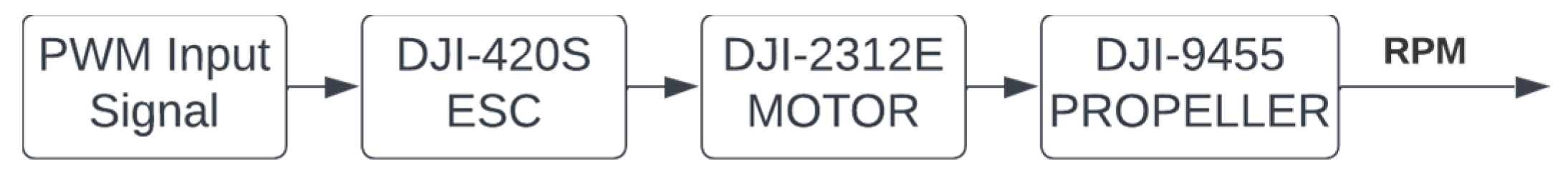
4.2. Experiment Setup and Data Collection for Analyzing the Propulsor Dynamics
The propulsion system dynamics depends on the performance of the motor, ESC, and the propeller, which is shown in
Figure 4. Therefore, the whole propulsion system will be excited, with the sweeping control input to obtain the transfer function instead of identifying only the motor and propeller.
From [
18,
19], the dynamics of the propulsor system could be represented by a first order transfer function where the inertia of the propeller dominates the response of the propulsor system. The transfer function of the electrical propulsor system is shown in this equation below:
The sweeping time domain data used for the system identification starts with the frequency of 1 rad/s and ends with 100 rad/s, and the data are sampled at 100 Hz, which is about 25 times faster than the bandwidth of the propulsor system, so that all the characteristic modes of the propulsor system will be captured.
4.3. Experiment Setup and Data Collection for the Bare-Airframe Dynamics
An X-Plane UAV model and DJI-450 UAV are constructed from the same CAD file, with the same physical specifications as described in
Figure 5. Then, both the X-Plane UAV model and DJI-450 UAV are excited with the pilot angle commands. The frequency spectrum of the pilot’s command is large enough to cover the natural frequency of the UAV bare-airframe dynamics. The pilot’s command signal, the controller’s output, and the angular rate output response of DJI-450 UAV and X-Plane UAV model are collected. The bare-airframe dynamics and identified transfer function of these two models in the longitudinal axis are obtained using the FRESPID and NAVFIT identification features in the CIFER software.
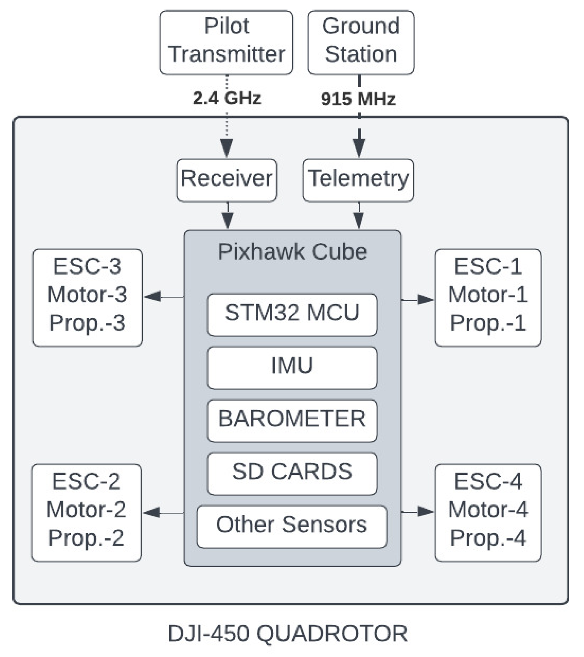
Since the VTOL UAV is not stable in nature, it needs a feedback controller to stabilize. From real flight tests, the required data should be collected for the system identification process. The Pixhawk Cube (version: black) hardware with Arducopter firmware v4.3.1 is chosen to build into controller. Pixhawk is an open-source system with well-developed and mature verifications (Pixhawk is available from
https://ardupilot.org/copter/docs/common-thecubeorange-overview.html (accessed on 1 June 2023). The Pixhawk has become the most popular system in professional communities all over the world.
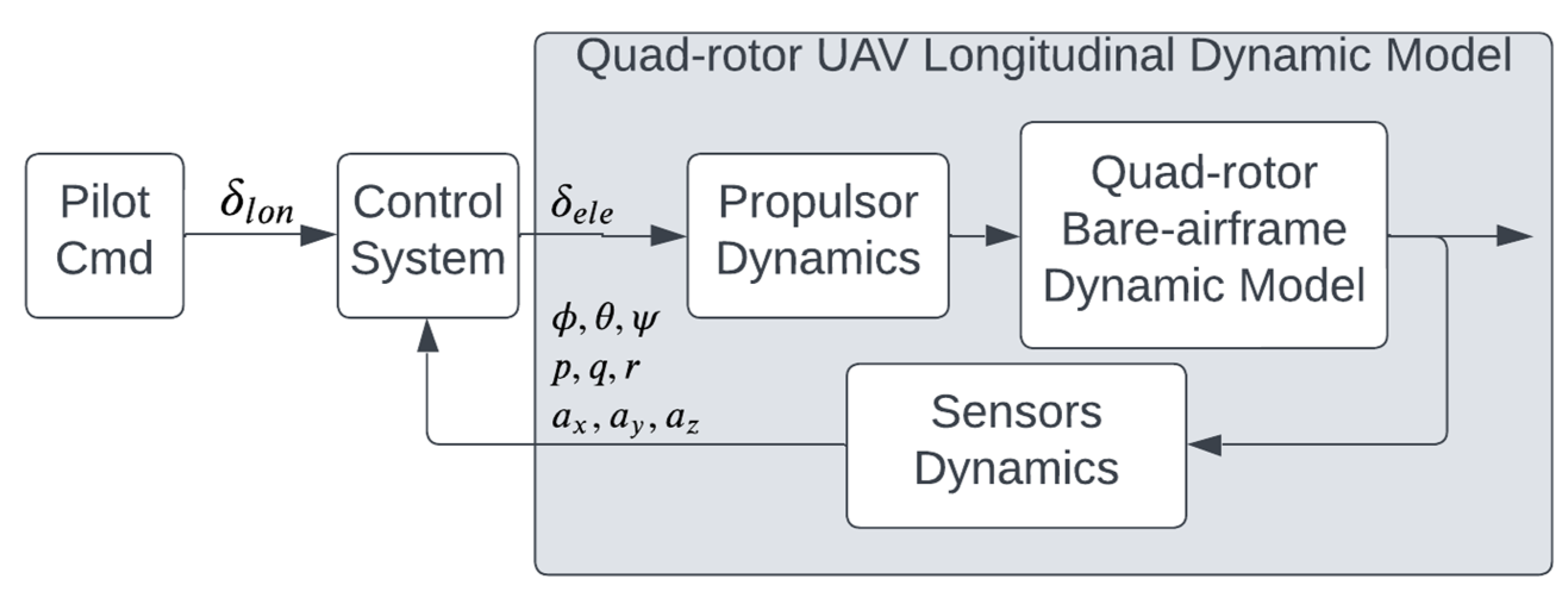
The simple PID controller is used to stabilize DJI-450 UAV, and the other parts of the closed-loop control are shown in
Figure 6. The Pixhawk Cube flight controller system is running the ArduCopter firmware. In Pixhawk, the pilot inputs are
with each axis control command
and angular velocity (p, q, r). The three-axis linear accelerations (
) are measured and logged at the high rate of 400 Hz. These high sampling rate data are imported to the CIFER software for system identification and validation processes to extract the UAV bare-airframe dynamics model.
The same closed-loop control architecture is constructed in Simulink to collect the flight data of the X-Plane UAV model, as shown in
Figure 6. The X-Plane UAV model communication interface is directly connected to the Simulink in order to have a minimal delay in data transfer between X-Plane and Simulink. This avoids the delay problem of the identified longitudinal dynamics of the quadrotor UAV in X-Plane.
For the purposes of this paper, the pilot commands, controller’s output, angular velocity, and the timestamp of the data in pitch axis are used to identify the bare-airframe dynamics of the quadrotor UAV both in X-Plane and in the real world.
From the datasheet, the control hardware of DJI-450 adopts a STM32 microprocessor with its peripherals, and two communication links of 2.4 GHz and 915 MHz, as shown in
Figure 5, with the flight controller setup in X configuration.
The most important factors that affect the result of the identification process are the natural frequency of the system and the sampling rate. Defining the right expected natural frequency of the VTOL UAV will make sure that the sweeping frequency range should be wide enough to cover the whole frequency range of the quadrotor UAV. Thus, all of the distinct modes of the open-loop longitudinal dynamics can be observed in the identified result. The sweeping frequency range is determined by the natural frequency of the identified vehicle [
14]. In this study, the natural frequency of the DJI-450 UAV is estimated from the UH-1H natural frequency using the Froude scale method. This method is widely used and has been proven in many flight test data [
10].
Using the Froude scale rule [
14], the natural frequency of the UAV is estimated from the UH-1 helicopter natural frequency and the ratio between the UH-1 blade diameter and the DJI-450 UAV hub-to-hub distance.
where the UH-1H natural frequency
from [
12] is 0.405 rad/s.
From the specifications of the UAV shown in
Table 1, both the X-Plane UAV model and the DJI-450 UAV have the same diagonal distance between the two motors. This is also known as a hub-to-hub distance of 460 mm, which is around 18 inches. The UH-1H propeller diameter is about 50 ft = 600 inches.
Therefore, the sweeping frequency range calculated from Equation (4) is:
Practically, the actual frequency range is expanded to [0.5, 20] rad/s to make sure that it covers the desired frequency range of the vehicle [0.75, 7.5] rad/s. The sweep signal total minimum time length is:
Following the instruction by Tischler et al. [
14] for the pilot sweeping signal to utilize the COMPOSITE function in CIFER for higher system identification quality, the pilot should make at least two sweeps with 5 s trim condition at the beginning, between and at the end of each sweep. Thus, the minimum flight time for the system identification process for the pitch/roll axis is:
In X-Plane, the chirp Z-transform signal generation block from the CONDUIT is used to simulate the pilot
signal. The equations used to generate the Chirp-z signal are described in Tischler et al. [
14] as below:
The second important parameter for a successful system identification process is the sampling rate. The experimental data must be logged at least 25 times faster than the desired natural frequency. The data are sampling at 25 times faster to ensure that there is enough room to add in a filter to the data at the post-processing step, in case the data need to be refreshed.
Once the desired sweeping frequency range is selected, the sampling rate can be calculated based on the highest value of the frequency range. In this study, the sampling rate is:
The data-logging rate of the Cube flight stack is 400 Hz, which should be much higher than the required sampling rate of 29 Hz. This high logging rate of the flight stack helps to avoid all the latency, aliasing, and data filtering problems along the identification process.
Following the strict requirements above guarantees a precise pilot input signal to exercise the dynamics mode of the vehicle and the logged data could capture all the modes of the DJI-450 UAV. The quality of the system identification process is quantified by the coherence value; a good result will have coherence >0.6 and an excellent result will have coherence value >0.8 [
14].
5. Experiment Result
5.1. Frequency Response of the Quadrotor with Respect to the CG Position
As is discussed at length in [
17], the X-Plane dynamics engine demonstrates remarkable precision in simulating the impact of the CG position on the longitudinal dynamics of the quadrotor UAV. As shown in
Figure 7, the quadrotor has pure divergent characteristics when the CG is above the propellers’ plane. This outcome significantly influences the design of the controller, as it plays a crucial role in achieving both excellent performance and handling quality.
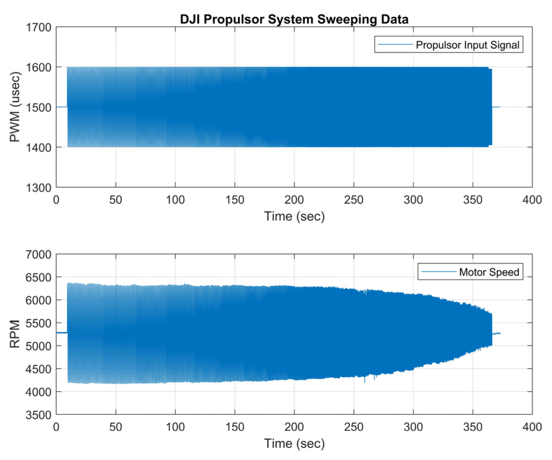
5.2. Frequency Response and Identified Transfer Function of the Electrical Propulsion System
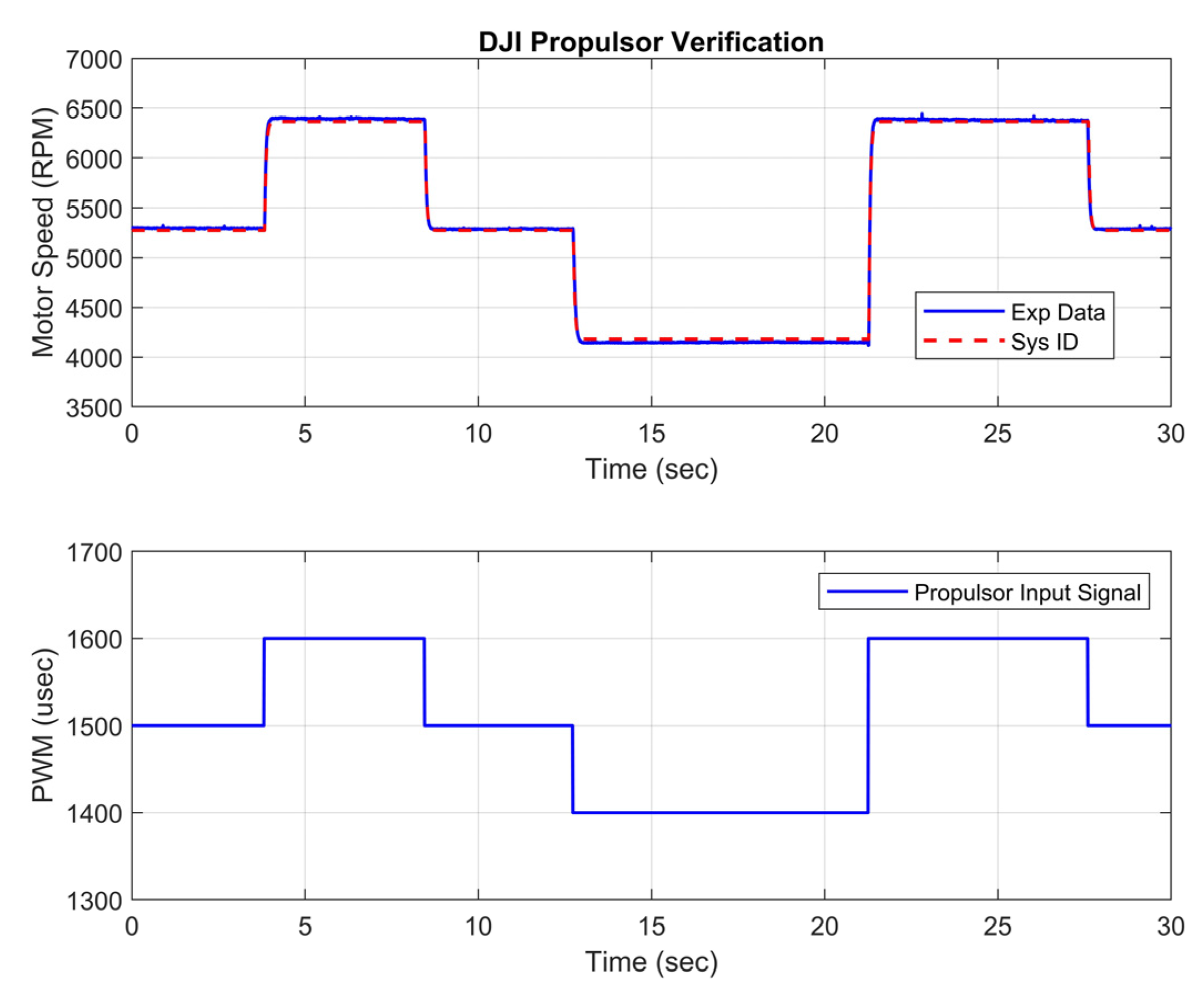
Figure 8 shows the time domain sweeping data used for extracting the frequency response of the propulsion system at 50% throttle, which is equivalent to the PWM input signal of 1500 (us) high time. The frequency response of the propulsion system has a very high coherence of almost one, which means that the identified result has a very high accuracy, as shown in
Figure 9. Then, the NAVFIT feature in CIFER is used to parametric fit the frequency response data to the transfer function of the propulsor system. The result is shown below:
It is obvious that when the scale of the UAV drone is increased, the size of the propeller will increase also, and the inertia of the propeller increases with the squared increment in diameter of the propeller. As a result, the pole of the propulsor system is smaller and approaches the bare-airframe characteristic poles. In a large, heavyweight UAV drone, the dynamics of the propulsion system play an important role in the dynamics of the overall UAV drone. Carefully characterizing the propulsor system dynamics and making sure that the propulsor system in the X-Plane model has the same characteristics will guarantee the similarity between the simulation results and the real-world flight data.
Finally, the model is verified with step-input time domain data and the result is shown in the
Figure 10 below:
5.3. Frequency Response and Identified Transfer Function of Longitudinal Bare-Airframe Dynamics of the Quadrotor UAV Model in X-Plane
In this section, a quadrotor UAV is built in X-Plane with exactly the same configurations and specifications as the DJI-450. The flight data are logged and input to CIFER software to extract the longitudinal dynamics of the vehicle.
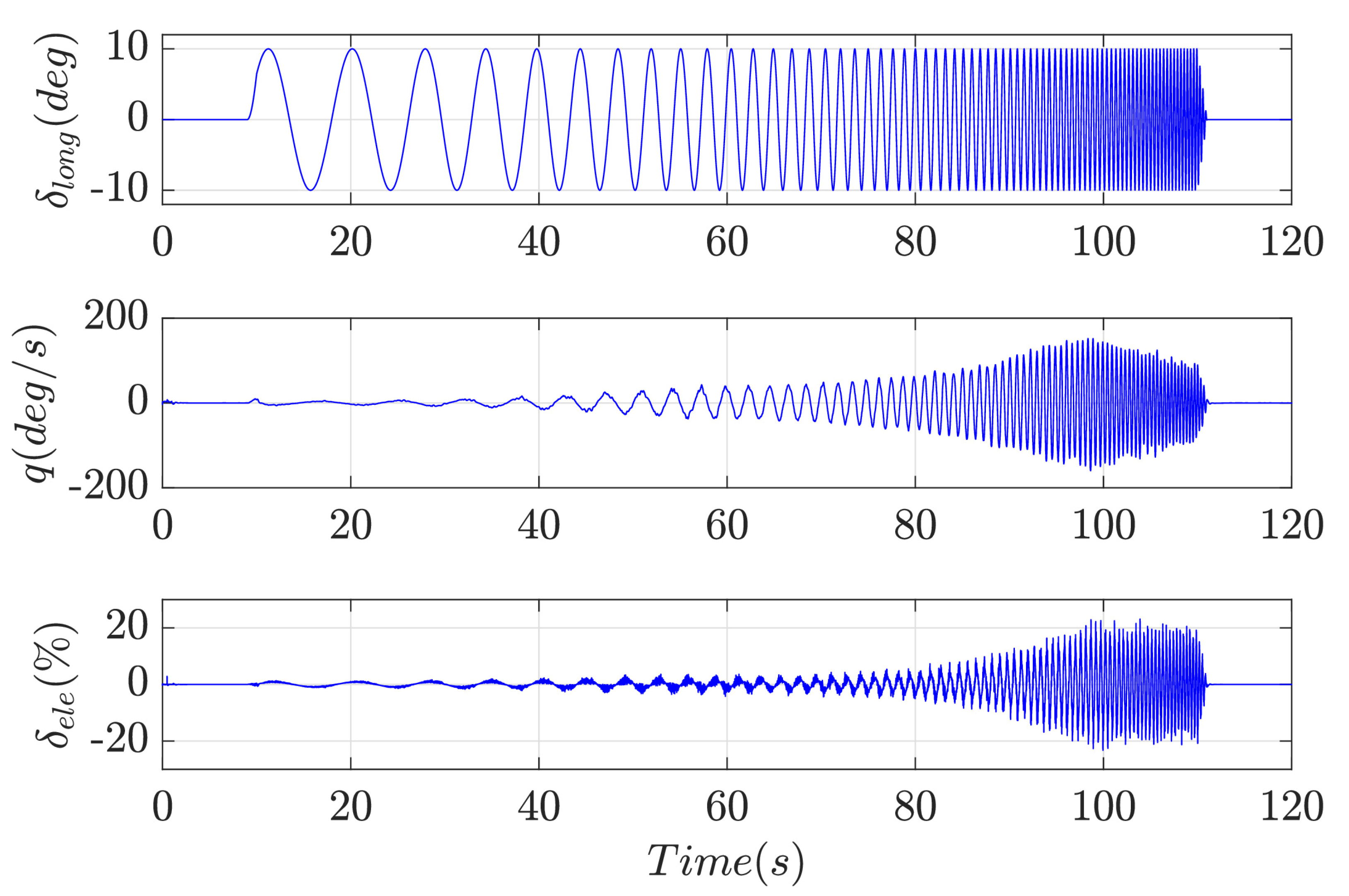
Figure 11 shows the time domain sweeping data of the quadrotor UAV in X-Plane. The top plot is the chirp-z signal from 0.7 to 20 rad/s with an amplitude of 10 degrees. The middle plot is the angular rate of the pitch axis, and the bottom plot is the control effort from the PID controller. Since the environment in the X-Plane simulator is ideal, with no wind disturbance, one sweep signal is enough to extract the bare-airframe dynamics of the quadrotor UAV. Then, the time domain flight data is used to extract the frequency response, and the identified model of the UAV model in X-Plane is shown in
Figure 12.
The coherence of the frequency response in
Figure 12 is larger than 0.8 for a frequency range of 1~20 rad/s. The high coherence implies that the dynamics of the UAV are greatly excited in pitch axis and the signal-to-noise ratio (SNR) is very high. Hence, the dynamics of the UAV in X-Plane could be represented by this frequency response.
The transfer function of X-Plane quadrotor UAV longitudinal dynamics can be presented as:
The transfer function identification cost of the X-Plane UAV model, as shown in
Figure 12, is 10.56. Based on the guidelines for cost J by Tischler et al. [
14], the identification cost of X-Plane J < 50, which is excellent. The errors between the identified model and frequency response in magnitude and phase at each frequency are calculated and plotted in
Figure 13. The error between the identified result and the frequency response is almost zero in the frequency range from 1 to 20 rad/s and the error does not exceed the ±95% confidence limit, which proves that the parameters are identified with high confidence.
The pitch dynamics of the VTOL UAV form an unstable system because its two complex poles are on the right-hand-side plane. The system is lightly damped and has a natural frequency of 2.42 rad/s. This natural frequency is very close to the expected natural frequency of 2.33 rad/s, which is calculated from the Froude scale. This means the physical simulation engine of X-Plane could capture the important metrics of the bare-airframe dynamics of the vehicle.
The transfer function of the X-Plane model in the longitudinal axis has a hover cubic structure (third order, one real pole and two complex poles), the same as the transfer function derived from the physics-based method by McRuer et al. [
6], which is proven with many real fight data, especially by Berrios et al. and Wei [
13] for the sub-scale quadrotor real flight data. This means that the physical engine inside the X-Plane is matched with the physics of the real-world environment.
These two complex poles on the right-hand-side plane with the non-zero imaginary parts show that the quadrotor UAV is an unstable system with oscillation. Given that the CG position is lower than the propeller plane in the X-Plane model, this unstable oscillation phenomenon is matched with the effects of CG position analyzed by Pounds et al. [
17]. This implies that an important effect of the CG is also captured by the X-Plane simulation engine.
The three important metrics (CG’s position, hover cubic structure, and the natural frequency) of the quadrotor UAV bare-airframe dynamics in X-Plane are matched with the dynamics of the real-world quadrotor UAV, which is analyzed in the literature [
7,
9,
13]. This result proves that the X-Plane physics engine simulator for the VTOL UAV is qualitatively verified to use as a tool to predict the bare-airframe dynamics of the actual DJI-450 UAV. Next, real DJI-450 UAV bare-airframe dynamics will be identified to compare with the X-Plane UAV model bare-airframe dynamics quantitatively.
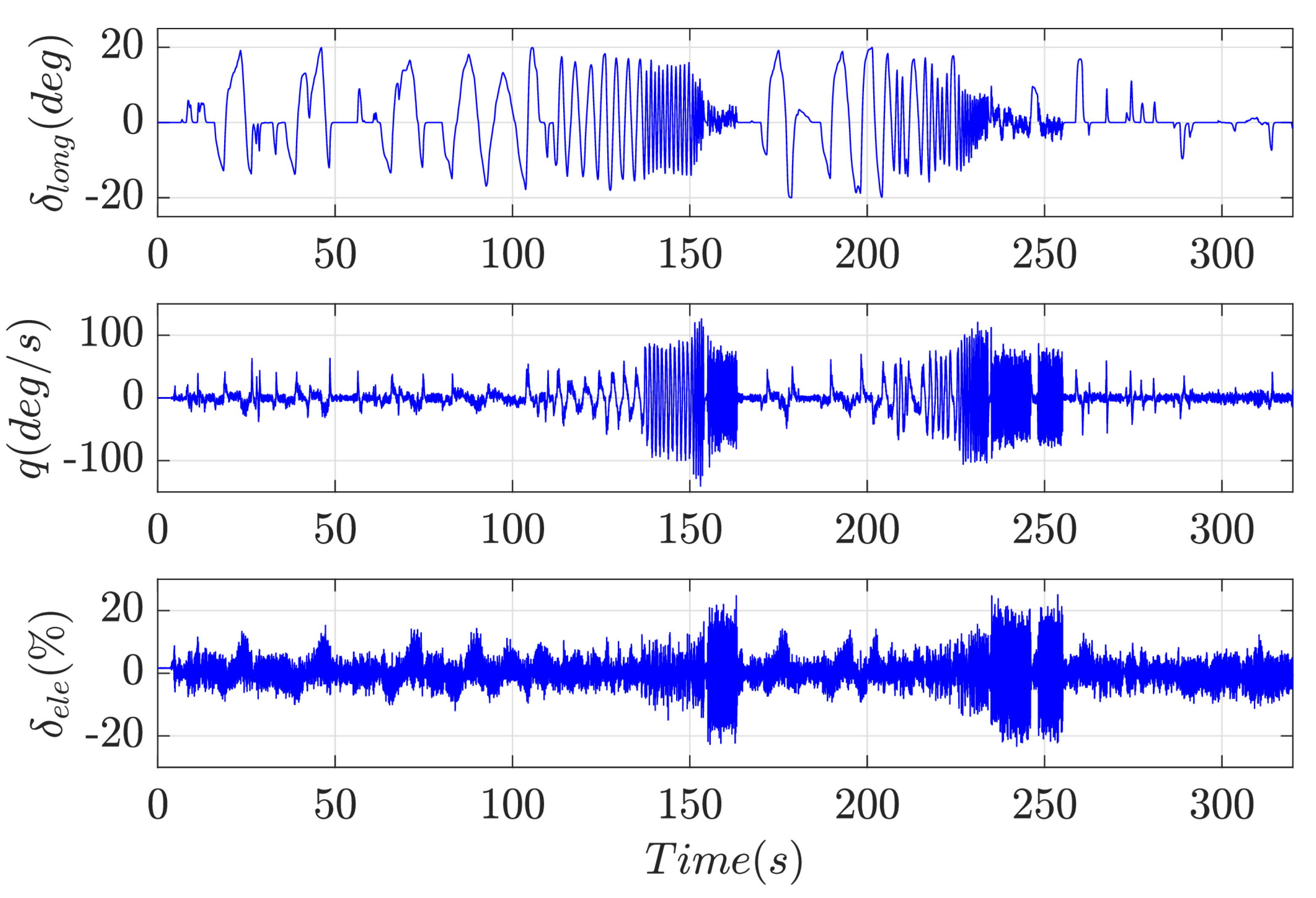
5.4. Frequency Response and Identified Transfer Function of Longitudinal Bare-Airframe Dynamics of the DJI-450 Quadrotor UAV in the Real World
In the same way as the identification process of the X-Plane UAV model,
Figure 14 plots the time domain real flight data used to extract the frequency response of the DJI-450 quadrotor. The top plot shows the two cycles sweep command of the pilot in the frequency range of 0.7–20 rad/s with an amplitude of 20 degrees in the 300 s time length. The amplitude of the sweep signal for actual flight with DJI-450 UAV is larger than the amplitude of the sweep command used for the X-Plane model. Since they are real flight data, there are inevitable wind disturbances from the environment. Thus, increasing the amplitude of the input command will enlarge the signal-to-noise ratio, which ensures the high coherence value of the identified frequency response of the DJI-450 UAV.
The middle plot in
Figure 14 is the pitch angular velocity of the DJI-450 UAV, and the bottom plot is the control effort of the PID controller for stabilizing and tracking the pilot sweeping command.
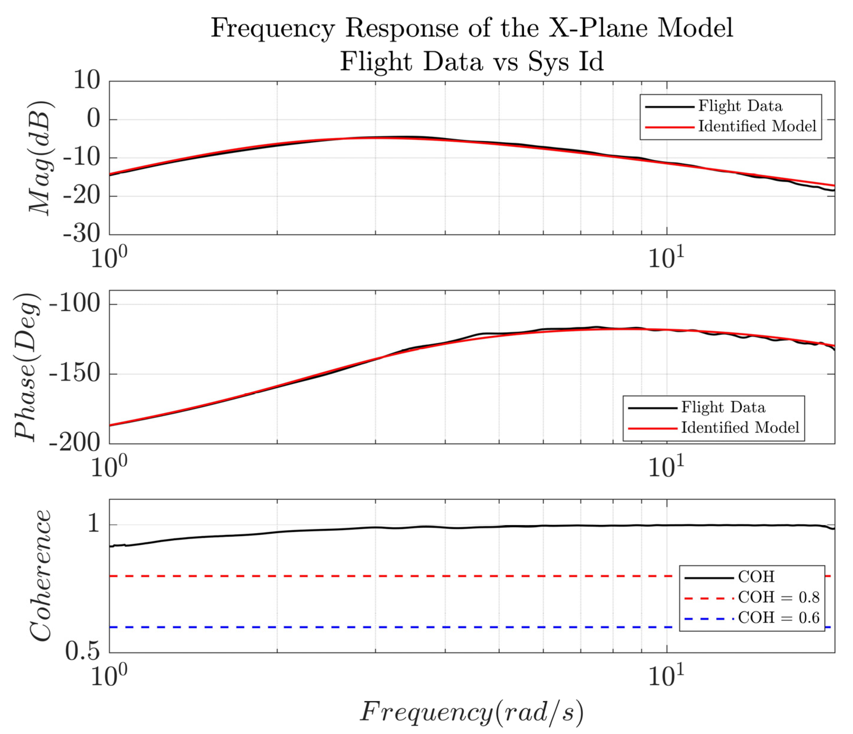
Figure 15 shows the frequency response and the parametric fit transfer function in pitch axis of DJI-450, which has excellent coherence of larger than 0.8 for the frequency range of 1–20 rad/s. This indicates that the frequency response is good enough to present the dynamics performance of DJI-450.
The transfer function of the longitudinal dynamics of DJI-450 is shown below:
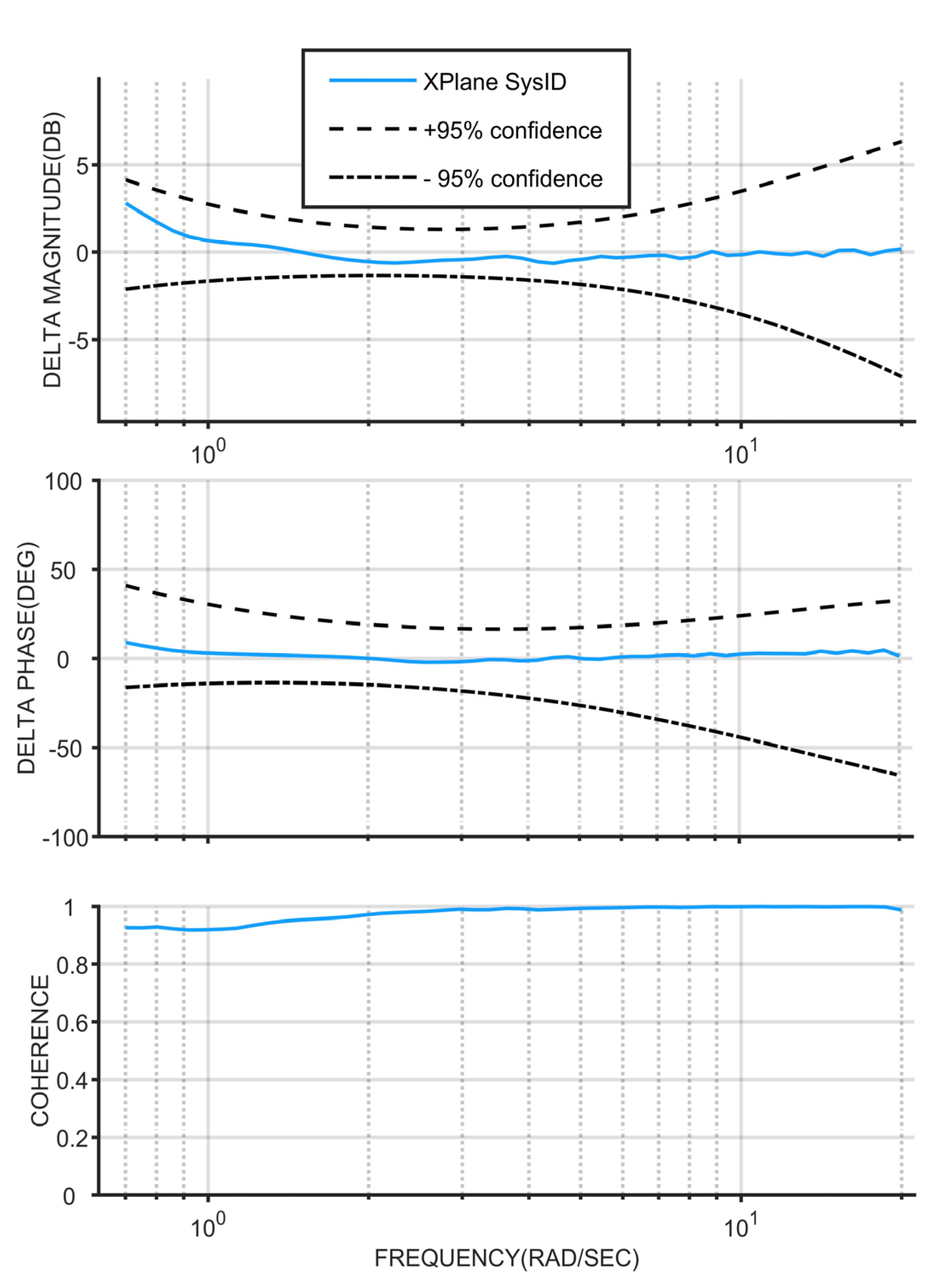
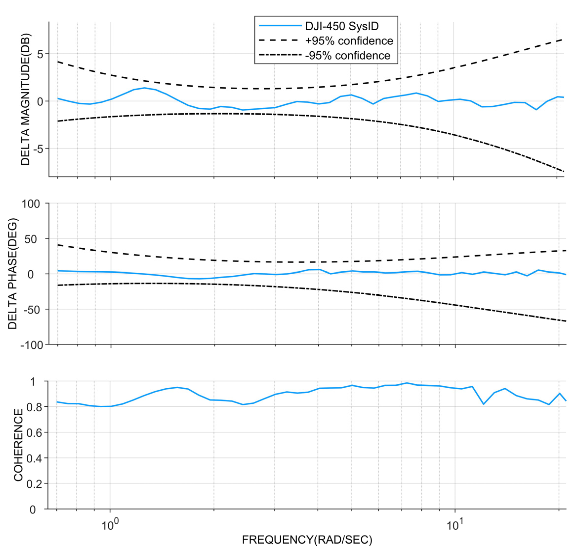
The error between the identified result and the frequency response of the DJI-450 model is almost zero and the error stays well inside the ±95% confidence limit, which proves that the parameters are identified with high confidence, as shown in
Figure 16.
5.5. Discussion
In this section, the frequency response and identified longitudinal bare-airframe dynamics of the quadrotor UAV model in X-Plane versus the DJI-450 quadrotor UAV in the real world will be compared to each other, and to other people’s work with the equivalent size of quadrotor UAV. Furthermore, the error of the bare-airframe dynamics of the UAV model in X-Plane and DJI-450 UAV will be quantified using the MAPE method.
In
Table 3, the transfer function identification cost J of DJI-450 UAV is 15.29, which is an excellent match with the guidelines J < 50 by Tischler et al. [
14]. This verifies the high accuracy of the identified parameters of the pitch dynamics. The transfer function of DJI-450 UAV matches with the bare-airframe dynamics of the X-Plane UAV model. DJI-450 UAV bare-airframe dynamics have an oscillatory unstable system because the system has two complex poles on the right-hand-side plane with damping coefficients of 0.54. The natural frequency of the system is 2.83 rad/s, which is very close to the natural frequency of 2.33 rad/s, calculating via the Froude scale. Although hover cubic function is intuitive, in some research the second order transfer function is used to fit the data instead of the hover cubic. Thus, an important characteristic of the vehicle is lost at the cost of simplicity, which leads to a low fidelity of the model and, as a result, this costs a lot of time and money for the controller design, testing, and verification phase in the future.
That both natural frequencies of the X-Plane and DJI-450 are close to 2.33 rad/s proves that using the Froude-scale method to estimate the natural frequency of the quadrotor is precise. The estimation of natural frequency plays an important role in not only designing the sweeping input signal, which can excite all the specific modes of the quadrotor longitudinal dynamics, but also in selecting the sampling rate of the system. In this research, the designed pilot input/chirp-z sweeping signal in the range of 0.5–20 rad/s, with a sampling rate of 400 Hz, could excite and capture/log all the dynamic modes of the UAV and the frequency response of X-Plane. From the tests, DJI-450 UAV is identified with a high confidence in its precision. The longitudinal dynamics of the X-Plane model and DJI-450 quadrotor are both plotted in
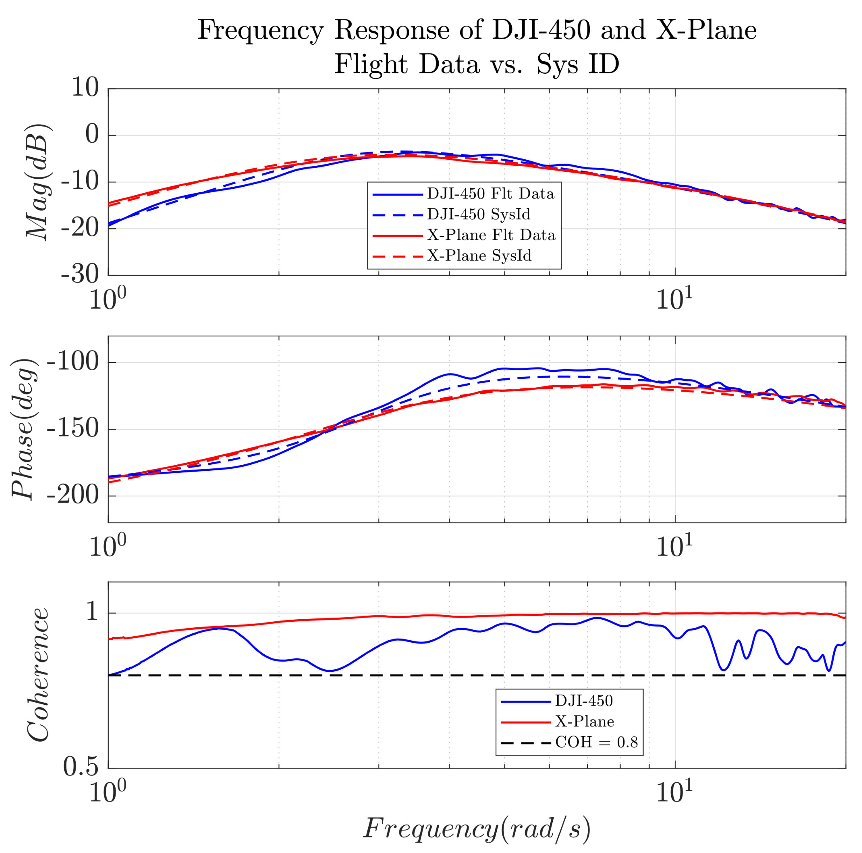
Figure 17. This indicates not only the quantitative comparison results but it also points out the similarity between these two models.
The frequency response of the X-Plane UAV model matches with the DJI-450 UAV model in 4~20 rad/s. In the low frequency region (0.7~4 rad/s) there is a small mismatch, which is inevitable in real flight tests. Wind disturbance at a low frequency will be significant. The angular rate command signal used for the system identification
is small because
depends on the value of frequency f. At a low frequency, f has a small value, and therefire the signal-to-noise ratio is lower than in the high frequency region, where f is now at larger value. This low signal-to-noise ratio makes DJI-450 coherence value in
Figure 17 smaller than the coherence value of the model in X-Plane, where the disturbance is always controlled to zero.
This mismatch does not mean that the X-Plane model is not precise. However, it indicates that the DJI-450 UAV frequency response is not as highly precise as X-Plane in the low frequency region because the X-Plane model has a very high coherence value of almost one, due to a controlled environment with no wind disturbance in X-Plane.
Furthermore, the bare-airframe dynamics of the UAVs in this study (X-Plane model, DJI-450) are compared with the dynamics of the quadrotor UAV of the same size from references [
12,
17] to validate the fidelity of the identified model. The summary of these UAV bare-airframe dynamics is shown in
Table 4. There are four dynamics data of the same size sub-scale quadrotor UAVs in
Table 4 with identical natural frequencies and damping ratio. Only slight differences in the value of the stable pole are found. This promising similarity in the dynamics of the quadrotor UAVs in
Table 4 builds up confidence in the high fidelity of the X-Plane physical simulation engine.
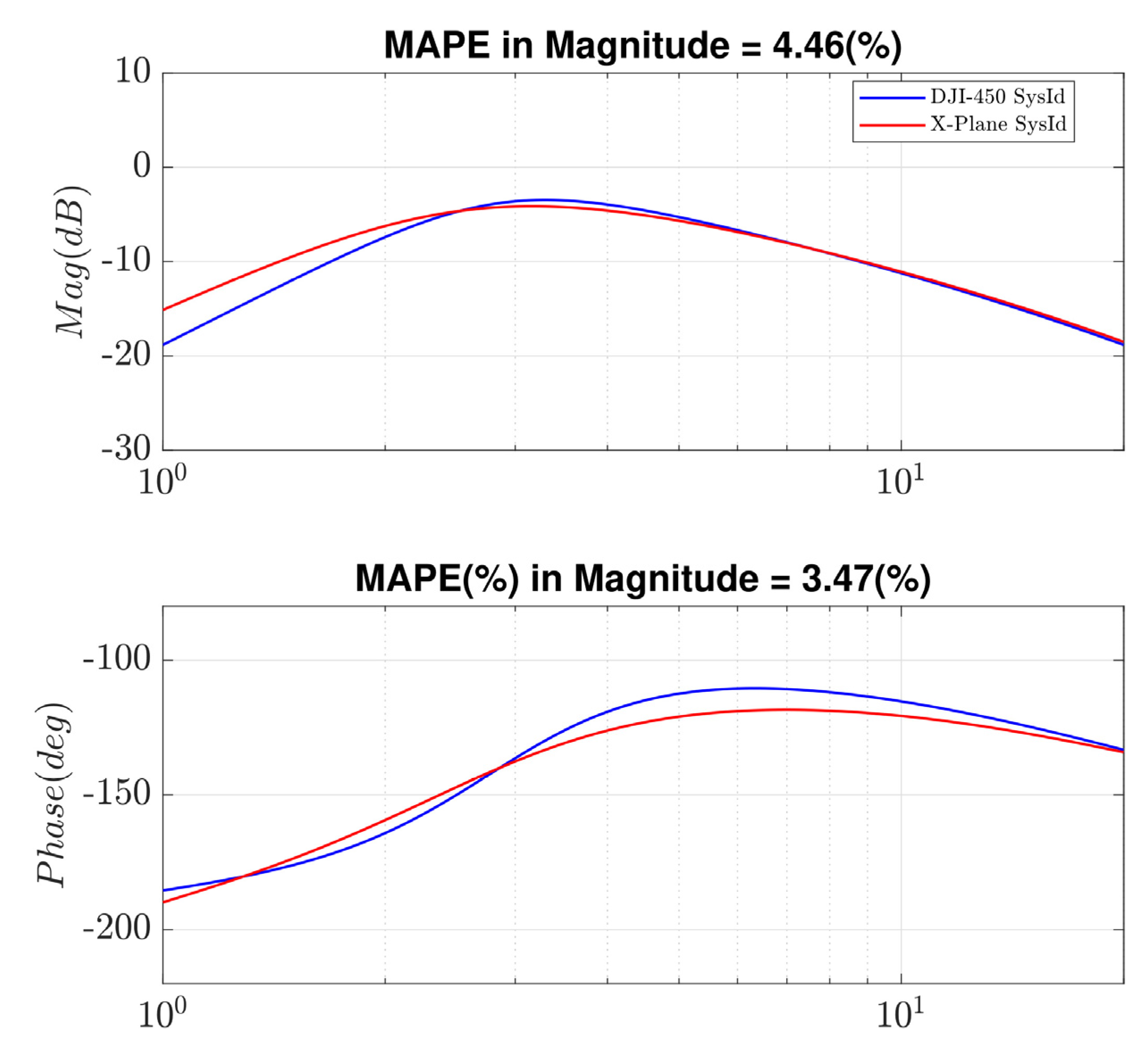
The error in identified longitudinal dynamics between the X-Plane UAV model and DJI-450 UAV is quantified using the Mean Absolute Percentage Error (MAPE) method as shown below:
where,
is the X-Plane magnitude data array, and phase data array.
is DJI-450 magnitude data array, and phase data array.
The purpose of this quantification is to validate the fidelity of the X-Plane physical simulation engine. From
Figure 18, the errors are 4.46% in magnitude and 3.47% in phase, and the total error is 7.93%, which also means that the fidelity of the X-Plane model is around 92% (100% − 7.93%). Therefore, the accuracy of the UAV’s longitudinal dynamics extracted from the X-Plane simulation engine could reach 92%. The result of 92% high fidelity for the X-Plane model is accurate enough to use in the proposed method to design a new VTOL UAV in
Figure 2.
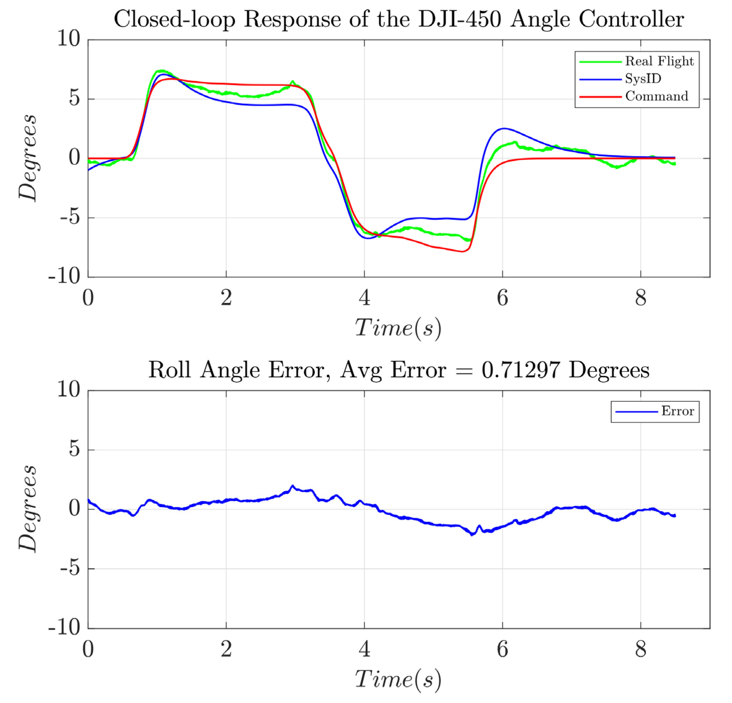
The transfer function of the bare-airframe longitudinal dynamics is used for the verification process. A doublet pitch angle command signal is utilized for the verification as shown in the
Figure 19 and
Figure 20. Both figures plot the pitch angle and the pitch rate in the top plot and plot the error between the measured flight data and the identified result in the bottom plot. The equations used to calculate the absolute error are shown in the equation below:
Figure 19 depicts the logged pitch angle from the real flight alongside the estimated pitch angle derived from the identified bare-airframe dynamics of the DJI-450 UAV in the pitch axis. The average error remains commendably low, approximately 0.8 degrees. This outcome is notable. The minor deviation can be attributed to the influence of wind disturbances.
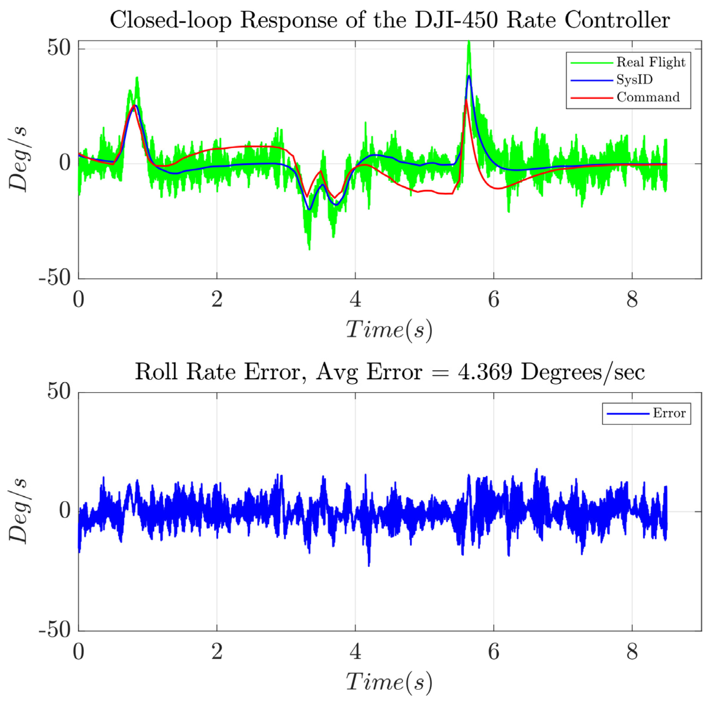
Figure 20 illustrates that the pitch rate derived from the identified model closely matches the actual flight pitch angle. The average error in pitch rate amounts to 4.369 deg/s, making it virtually impossible for the pilot to distinguish any difference between flying the DJI-450 UAV in the real world or flying in the simulation.
In addition to achieving a 92% accuracy, shown in
Figure 18, in predicting the DJI-450 UAV’s longitudinal bare-airframe dynamics with X-Plane, the verification process yielded outstanding results, with an average error of 0.8 degrees in pitch angle and 4.369 deg/s in pitch rate. These findings confirm that the proposed method, which combines X-Plane and CIFER, can significantly reduce the time and cost involved in the UAV design phase. Moreover, the precisely identified model is qualified to be used for the flight controller, which would not only cut the cost and time of the new UAV design phase, but also reduce the cost of flight controller development and testing phase tremendously.
6. Conclusions
The longitudinal dynamics of a quadrotor UAV in X-Plane and in the real world (DJI-450) are successfully extracted using frequency domain system identification software, named CIFER, to validate the physics engine of the X-Plane simulator. This research result proves that the internal flight dynamics engine of X-Plane is accurate. The X-Plane flight dynamics engine captures all of the four most important physical characteristics, such as the effects of the CG position, the electrical propulsor dynamics, the Froude scaled natural frequency estimation, and the hover cubic form transfer function of the VTOL UAV. These four parameters are the key ways to keep the X-Plane identified dynamics model the same as the quadrotor dynamics model in the real world. As the X-Plane physics engine fidelity is validated and qualified, the open-loop longitudinal dynamics of the DJI-450 UAV model in X-Plane and DJI-450 quadrotor in the real world are obtained and compared to each other. From the proposed method and procedures, minor iterations can obtain a significant and confident result toward an expected design outcome. The result is that the X-Plane simulator could accomplish a 92% high fidelity accuracy model, which is shown in
Figure 18. As a result, it would be no issue to use this method for obtaining the larger scale UAV without building the UAV in the real world. This high-accuracy UAV model in X-Plane is a new game changer with the ability to help industries design and produce bigger, heavier drones for wider applications at an extremely low cost and time expenditure compared to the traditional method, which requires a revision in hardware and flight test in each design iteration.
Furthermore, there is an impressive outcome from the verification results shown in
Figure 19 and
Figure 20, with an average error of 0.8 degree in pitch angle and 4.37 deg/s in pitch rate. These amazing results prove that the CIFER is a reliable frequency-domain-based system identification tool for the bare-airframe dynamics of UAVs, especially unstable systems like the VTOL UAVs, which is a very hard task for other time-domain-based system identification tools.
By leveraging the combined utilization of X-Plane and CIFER, the proposed method enhances the iterative design process of VTOL UAVs by accurately forecasting the bare-airframe dynamics of the vehicle, all without the need for physical construction and testing as is used in the traditional UAV design progress. This approach significantly lowers the time and cost of accomplishing UAV design. The UAV markets could capitalize on this technique to design and enhance UAVs to meet the evolving demands for bigger, heavier UAVs for a wide range of drone applications in the present era.


