Model-Free Guidance Method for Drones in Complex Environments Using Direct Policy Exploration and Optimization

Abstract

In the past few decades, drones have become lighter, with longer hang times, and exhibit more agile performance. To maximize their capabilities during flights in complex environments, researchers have proposed various model-based perception, planning, and control methods aimed at decomposing the problem into modules and collaboratively accomplishing the task in a sequential manner. However, in practical environments, it is extremely difficult to model both the drones and their environments, with very few existing model-based methods. In this study, we propose a novel model-free reinforcement-learning-based method that can learn the optimal planning and control policy from experienced flight data. During the training phase, the policy considers the complete state of the drones and environmental information as inputs. It then self-optimizes based on a predefined reward function. In practical implementations, the policy takes inputs from onboard and external sensors and outputs optimal control commands to low-level velocity controllers in an end-to-end manner. By capitalizing on this property, the planning and control policy can be improved without the need for an accurate system model and can drive drones to traverse complex environments at high speeds. The policy was trained and tested in a simulator, as well as in real-world flight experiments, demonstrating its practical applicability. The results show that this model-free method can learn to fly effectively and that it holds great potential to handle different tasks and environments.

1. Introduction

The recent advancements in drone technology have resulted in their widespread adoption across various industries worldwide. Drones offer favorable properties that make them highly suitable for complex mission environments, such as search and rescue operations in forests [1,2,3] and bridge inspections [4,5]. These environments often present challenges such as cluttered obstacles and weak communication and satellite signals. In search and rescue (SAR) tasks, it is crucial for drones to navigate around obstacles efficiently and reach their destinations quickly. In this study, we focus on the navigation problem of drones operating in unknown and complex environments, where they encounter various obstacles and reach their destinations quickly and safely. To maximize the maneuverability of drones while ensuring flight safety, researchers typically divide the controller into two layers: a low-level angular rate and attitude layer, analogous to the human epencephalon; and a high-level velocity, position, and navigation layer, resembling the human brain [6,7,8]. Among these parameters, the low-level control problem has been extensively analyzed, and accordingly, optimal solutions have been established. However, some issues still persist in high-level control methods, hindering the effective utilization of the high maneuverability of drones.

Based on extensive research, several factors have been identified as reasons for the improper utilization of the high maneuverability of drones. A recent study identified the latency of perception sensors, such as monocular and stereo cameras, as a contributing parameter [9]. It discussed the effect of perception latency in high-speed movement robot platforms. The study proposed a general analysis method to evaluate the maximum latency when operating the robot at the ultimate velocity. It highlighted that simply reducing the longitudinal velocity does not necessarily guarantee the security of the robot. However, this method can only adjust the latency tolerance, and the suggested solution is to use more advanced sensors, such as event cameras. In contrast, reducing the latency of software and algorithms is a more economical approach. Another study introduced a low-level multi-sensor fusion algorithm, where vision and three-dimensional (3D) lidar data were segmented [10]. Here, the core control system received and fused their results to reduce latency.

In addition to the factors mentioned above, the issue of coordination after modularization is a significant challenge. Traditional navigation pipelines for drones in unknown environments are typically divided based on perception, path planning, and control subtasks to solve the autonomous flight problem in a step-by-step manner [11,12,13,14,15,16]. A recent study proposed visual stereo simultaneous localization and mapping (SLAM) for drones, which accelerates the mapping process and thus provide an approach for map maintenance with a uniform distribution [17]. The problem of high-quality 3D mapping was addressed using only onboard, low-computing consumption, and imperfect measurements [18,19,20]. Some researchers focused on path planning using length analysis, search-based, and Euclidean signed distance field methods [21,22,23]. The control subtask has a long history, and there are many well-known and effective algorithms, such as PID, H-infinite, sliding mode control, and model predictive control (MPC) [24]. These methods enable drones to accomplish the tasks mentioned above through a parallel cooperation pipeline of components. Thus, it makes the entire system interpretable and facilitates the tuning of the parameters of each component. Although it may seem attractive from an engineering implementation perspective, due to the sequential nature, the communication latency between components and wastes computing resources on unnecessary functions is overlooked, leading to difficulties in achieving agile flight.

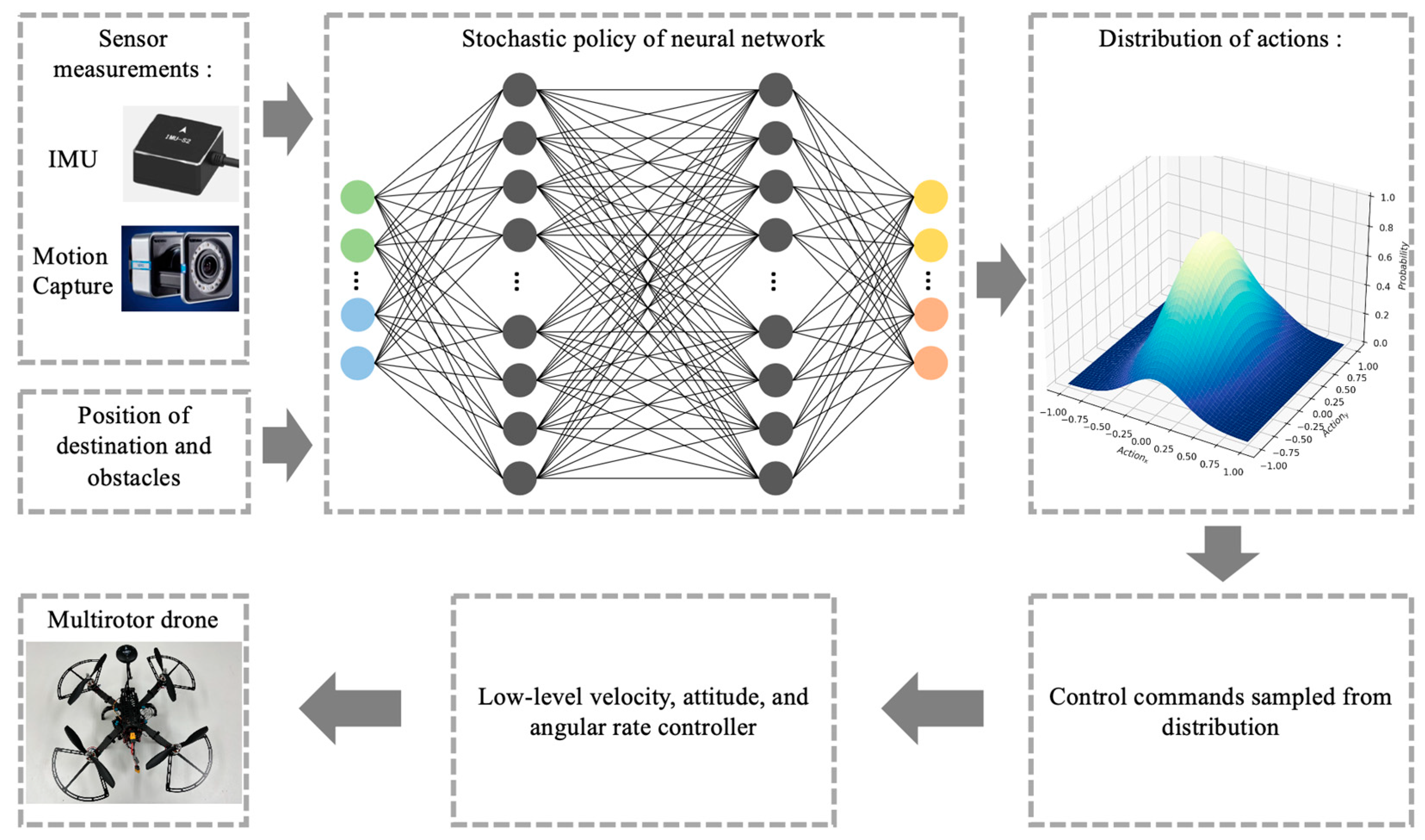
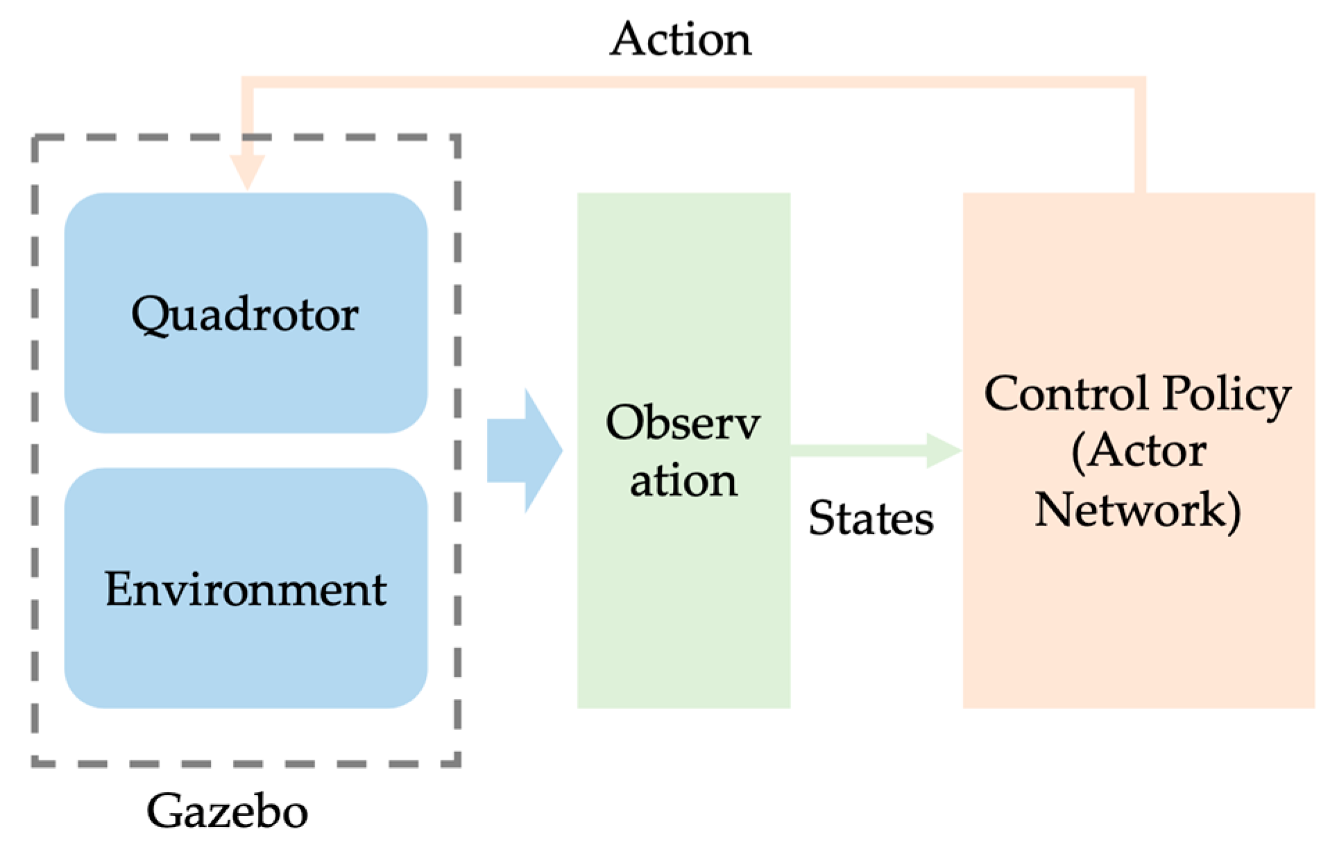
Thus, we propose a new guidance framework with a reinforcement-learning-based direct policy exploration and optimization method to maximize the maneuverability of drones and enhance flight speed in complex environments. In this framework, the low-level angular rate, attitude, and velocity are controlled by a well-tuned cascade PID, while the high-level path planning, position controller, and trajectory tracking controllers are merged into a control policy. The policy is a fully connected three-layer neural network that takes sensor measurements as inputs and outputs the distribution of the target velocity commands. Finally, the real control commands are sampled from the distribution and sent to a low-level controller, as shown in Figure 1. The main contributions of this study are summarized as follows:

Figure 1. Proposed RL controller.

• A novel navigation framework is proposed to improve the flight speed of drones in complex environments. The framework integrates an RL-based policy to replace the traditional path planning and trajectory tracking controllers in a conventional drone guidance pipeline. The experimental outcomes in both the simulated and real-world environments show that it can push the maneuverability of drones to the physical limit.
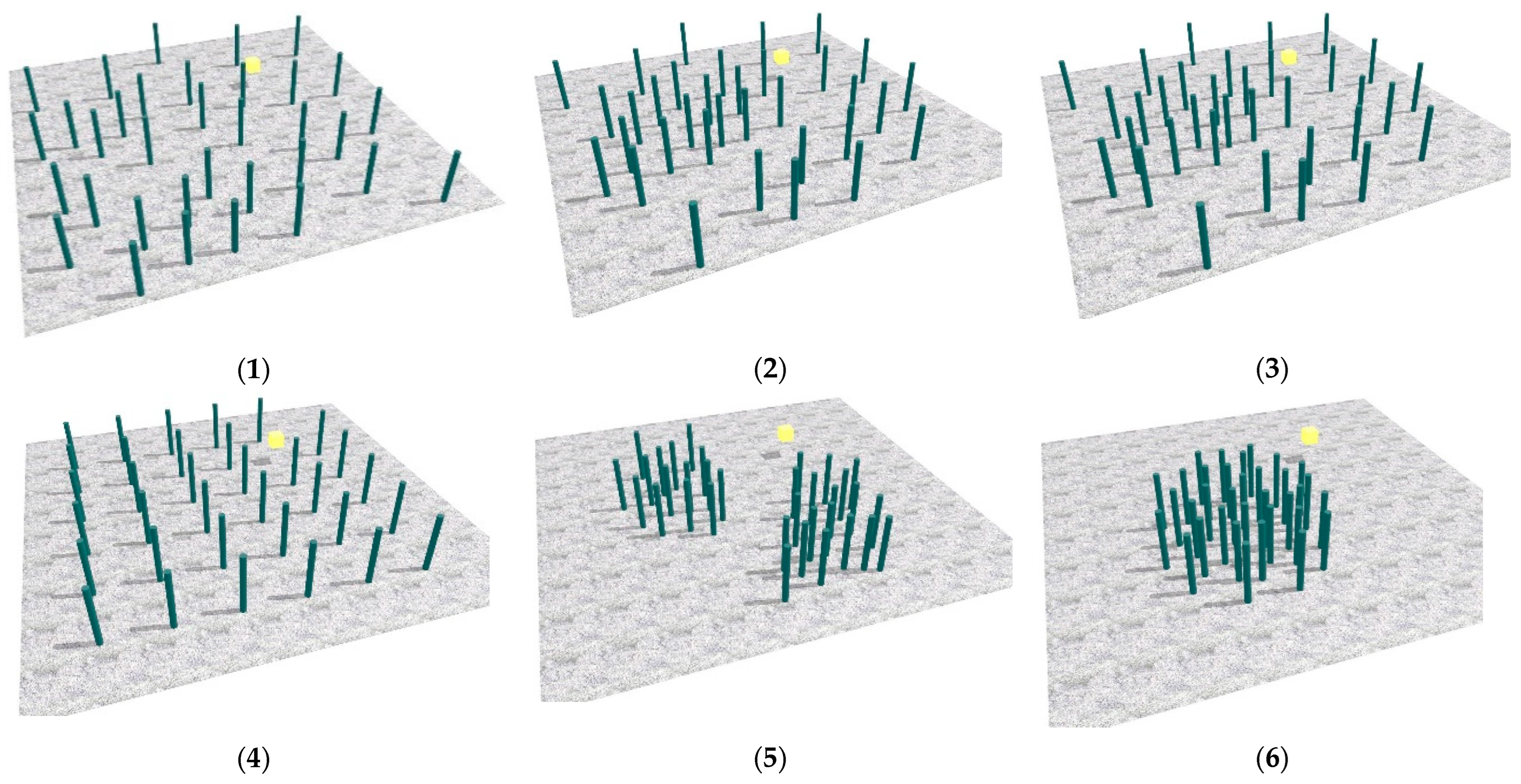
• A novel direct policy exploration and optimization method is proposed, which eliminates the need for a teacher–student structure commonly used in imitation learning and does not require reference trajectories. To train the policy, multiple environments (Figure 2) with varying obstacle distribution characteristics were created. Subsequently, the well-trained policy is directly applied to real-world drones for practical applications.
  

  Figure 2. Part of designed clutter environments. Yellow boxes indicate destination. Drones takeoff on left bottom of floor. (1) has randomly distributed obstacles, (2,3) have designed routes to traverse. (4) has neatly arranged obstacles, while (5,6) have clusters of obstacles.
• From a practical perspective, we designed a hybrid reward function to facilitate policy exploration and self-improvement. This function further comprises multiple continuous and discrete functions that can effectively evaluate the distance between the drone and the destination, energy consumption, collision risk with obstacles, and other such factors.

The remainder of this paper is structured as follows. Section 2 discusses the classical perception–planning–control pipeline and the latest RL works. Section 3 describes the low-level model-based attitude controller and high-level planning-tracking strategy in our approach, along with the designed reward function and the algorithm for direct policy exploration and optimization. Section 4 shows the experiments that were conducted to train and test the policy of the proposed structure in a simulator. We also applied this method directly to real-world drones and analyzed the observed advantages and limitations. Finally, the conclusions, opportunities, and challenges of future work are discussed in Section 5.

2. Related Works

2.1. Conventional Sequential Method

Flying drones in complex environments is a challenging task. The traditional approach involves breaking it down into specific problems, such as perception, path planning, and control, addressing them separately, and then arranging them in a sequential pipeline, as shown in Figure 3.

Figure 3. Pipeline of conventional method.

The main task of the perception module is to estimate the state of the drone and its surrounding environment using onboard or external sensor data. A few common and well-known perception algorithms include the SLAM and the visual–inertial odometry (VIO). The planning module generates a feasible and time-optimal trajectory that helps the drone accomplish its mission based on the state, environmental information, and task requirements. In a recent study, this module was classified into four types—sampling-based, search-based, optimization-based, and polynomial and spline trajectory-based. A control module typically operates at higher frequencies. This module calculates the corresponding control commands that enable the drone to follow the intended trajectory based on the state of the drone and target trajectory. Algorithms such as MPC can even predict the future states of a drone based on the motion model to search for optimal control inputs over the entire time window.

Although the conventional pipeline has enabled the autonomous flight of drones in complex environments, a few challenges still persist. For instance, although the VIO algorithms are lightweight, they require considerable computational resources. Planning algorithms may be affected by factors such as unmodeled system delays, state estimation drift, and discontinuities in perception modules, and this may result in suboptimal paths or even mission failures.

2.2. Reinforcement Learning

Reinforcement learning (RL) aims to learn how to make optimal decisions and maximize cumulative rewards through the interaction between an agent and its environment. Based on the optimization objective, RL can be divided into two types: value-based and policy-based methods. Different from the well-known deep learning, RL can update the knowledge of agents through trial and exploration in the world (a widespread structure like that in Figure 3) without a supervisor; this characteristic endows RL with vast potential to outperform human experts in computer games [25,26]. The primitive table-based RL algorithm can only deal with problems that only have discrete, limited states and actions. After this decade of developments, especially in relation to the combination of neural network technique, the RL can handle complex and nonlinear systems which have continuous states and actions; it is the foundation of applying RL to control and navigation tasks [27].

In recent years, learning-based methods have been extensively used in perception [28], planning [14], and control [29]. The neural networks can handle high- and low-dimensional information and are easy to deploy. Researchers have successfully replaced certain modules in classical pipelines with learning-based approaches, leading to significant advancements. The RL can update the knowledge of agents through trial and exploration worldwide (a common structure is shown in Figure 4) without a supervisor. Driven by this characteristic, it may potentially surpass human expert performance [30].

Figure 4. RL structure.

There are many variations in RL and value-based methods, including Q-learning, deep Q-network, policy-based deterministic policy gradient, trust region policy optimization [31], and proximal policy optimization (PPO) [32]. As shown in Figure 4, the agent interacts with the world over time, receives a state $s_t$ in the state space S at timestep t, and selects an action $a_t$ from the action space A; the mapping relationship from $s_t$ to $a_t$ is the policy $\pi \left(s_t|a_t\right)$. The world will transfer to a new state $s_{t+1}$, submit to the state transition probability $P\left(s_{t+1}|s_t,a_t\right)$, and present the agent with a scalar reward $r_t$ according to the reward function $R\left(s,a\right)$, which is affected by the model of the system or environment dynamics. After a complete interaction process (one episode) between the agent and the environment, a series of observations, referred to as trajectory $\tau =\left(s_0,a_0,s_1,a_1,\dots \right)$, may be obtained. We assume that this series process satisfies the Markov property $P\left(S_{t+1}=s_{t+1}|S_{0:t}=s_{0:t}\right)=P\left(S_{t+1}=s_{t+1}|S_t=s_t\right)$, which means that for a stochastic process, given the current state and all past states, the conditional probability distribution of its future states depends only on the current state.

2.3. Value-Based Methods

During an episode of continuous state transition and action execution, an accumulated reward (referred to as return), with the discount factor $\gamma \in \left(\mathrm{0,1}\right]$, was defined as:

$$R_t={\displaystyle \sum _{j=0}^{\infty }}{\gamma }^k{r}_{t+j}$$

(1)

The return can evaluate whether the entire process is good and helps the agent improve by maximizing the expectation of $R_t$. When a system model or state transition function is available, the optimization problem may be solved through dynamic programming. However, this is usually attainable. In this case, the complete trajectory cannot be obtained through model iterations, and the RL possesses the ability to solve this problem through trial and error. We define a value function to measure the value of each state, which is the expectation of the returns of trajectories starting from the current state and following policy $\pi$:

$$V_{\pi }\left(s\right)=E\left[R_t|s_t=s\right]$$

(2)

The action–value function for action $a$ in state $s$ following the policy $\pi$:

$$Q_{\pi }\left(s,a\right)=E\left[R_t|s_t=s,a_t=a\right]$$

(3)

The Bellman equation can be obtained by decomposing the expectation in $V_{\pi }$:

$$V_{\pi }\left(s\right)=\sum _a\pi \left(a|s\right)\sum _{s^{\prime },r}p\left(s^{\prime },r|s,a\right)\left[r+\gamma V_{\pi }\left(s^{\prime }\right)\right]$$

(4)

The optimal value function is the maximum value of the current state $s$ following an arbitrary policy:

$$V_{*}\left(s\right)=\underset{a}{\mathit{max}}{\displaystyle \sum _{s^{\prime },r}}p\left(s^{\prime },r|s,a\right)\left[r+\gamma V_{*}\left(s^{\prime }\right)\right]$$

(5)

The optimal action value function is:

$$Q_{*}\left(s,a\right)=\sum _{s^{\prime },r}p\left(s^{\prime },r|s,a\right)\left[r+\gamma \underset{a^{\prime }}{\mathit{max}}{Q}_{*}\left(s^{\prime },a^{\prime }\right)\right]$$

(6)

The intuitive solution to the RL problem is to find an optimal value function or optimal action–value function and always choose the action that motivates the system to transition to optimal states that can maximize the return of the trajectory. By estimating and updating these value functions, the agent can accurately evaluate the values of different states and actions and thus make optimal decisions through continuous learning. This approach is commonly referred to as value-based reinforcement learning. It also yields good results in application-based scenarios, such as aerial manipulator control [33], robot path planning [34], and lane following of unmanned cars [35]. However, as stated by Zhang in [36,37], the value-based method yields low training efficiency and data sufficiency; it requires several tricks and modifications to improve training speed and stability in practical and complex scenarios. We analyzed the reasons for this problem. The goal of the value-based method is to determine an optimal value function that defines the mapping relationship between actions and states once the algorithm converges. Each state has a corresponding action. However, the optimality of the action is questionable when the environment changes slightly. This is more apparent when the state and action spaces become significantly vast because the value function is unavailable for approximation.

2.4. Policy-Based Methods

Contrary to the approach of searching for an optimal value function, policy-based methods can directly optimize the policy $\pi \left(a|s;\theta \right)$ to enable it to choose the correct action in various states. Here, $\theta$ can be viewed as a parameter of a function approximation, and updating it through gradient ascent can improve the policy. This method usually performs better than value-based methods, particularly in complex scenarios with high-dimensional states and action spaces, and it possesses better convergence properties. The primary benefit of the policy-based method is that it can use a stochastic policy that exploits exploration. The value-based method has a deterministic policy that always chooses an action that can maximize the value function. This method only improves policy implicitly and does not possess exploration. Researchers usually solve this using $ϵ$-greedy exploration, which is insufficient and introduces extra hyperparameters. By assuming that the policy $\pi \left(a|s;\theta \right)$ is derivable and has analytical gradient, we obtain:

$${\nabla }_{\theta }\pi \left(a|s;\theta \right)=\pi \left(a|s;\theta \right)\frac{{\nabla }_{\theta }\pi \left(a|s;\theta \right)}{\pi \left(a|s;\theta \right)}=\pi \left(a|s;\theta \right){\nabla }_{\theta }\mathrm{l}\mathrm{o}\mathrm{g}\pi \left(a|s;\theta \right)$$

(7)

where, ${\nabla }_{\theta }\mathrm{l}\mathrm{o}\mathrm{g}\pi \left(a|s;\theta \right)$ is the likelihood ratio or score function. The policy gradient is defined as:

$$\nabla J_{\theta }=E_{\pi ,\theta }\left[{\nabla }_{\theta }\mathrm{l}\mathrm{o}\mathrm{g}\pi \left(a|s;\theta \right)Q_{\pi ,\theta }\left(s,a\right)\right]$$

(8)

We update policy parameters $\theta$ in k iteration step along the policy gradient. Here, $\alpha$ is the learning rate:

$${\theta }_{k+1}={\theta }_k+\alpha \nabla J_{\theta }$$

(9)

3. Method

As mentioned previously, we propose a new framework for guiding drones in complex environments. In the Section 1, we introduce a model-based attitude controller. The Section 2 presents the proposed method of direct policy exploration and optimization, which replaces the planning and trajectory-tracking modules in a classical pipeline. The Section 3 describes the designed reward function, which provides an effective evaluation criterion for policy optimization.

3.1. Low-Level Controller

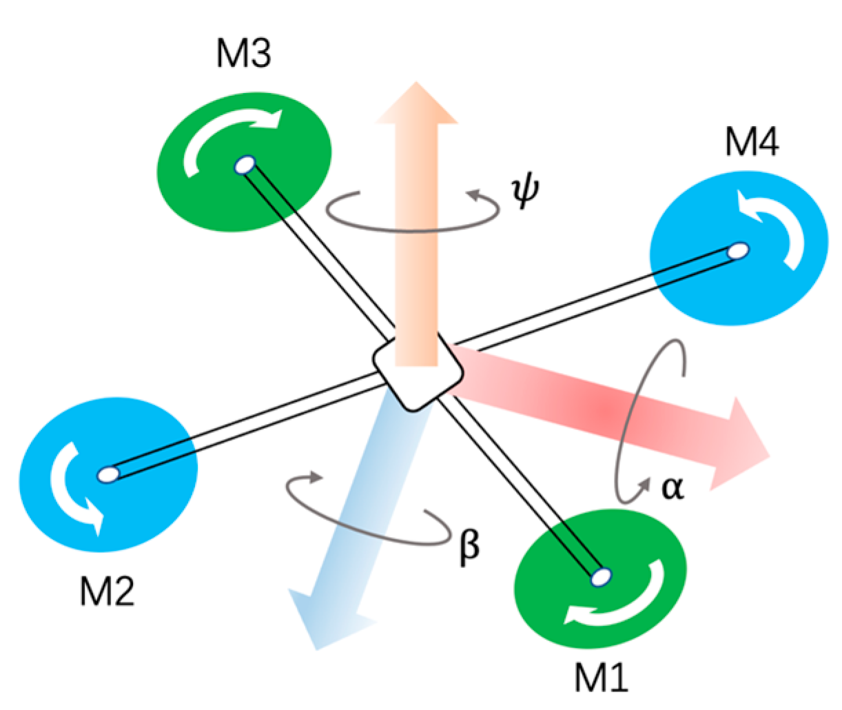
Drones are typically agile, and they possess a six-dimensional motion capability, 3D position (denoted by $Pos={\left[x,y,z\right]}^T$), and 3D orientation (denoted by $Rot={\left[\alpha ,\beta ,\psi \right]}^T)$, as shown in Figure 5. In our method, the low-level controller keeps the drone stable and agile, and precisely executes velocity commands from the high-level RL controller.

Figure 5. Drone model.

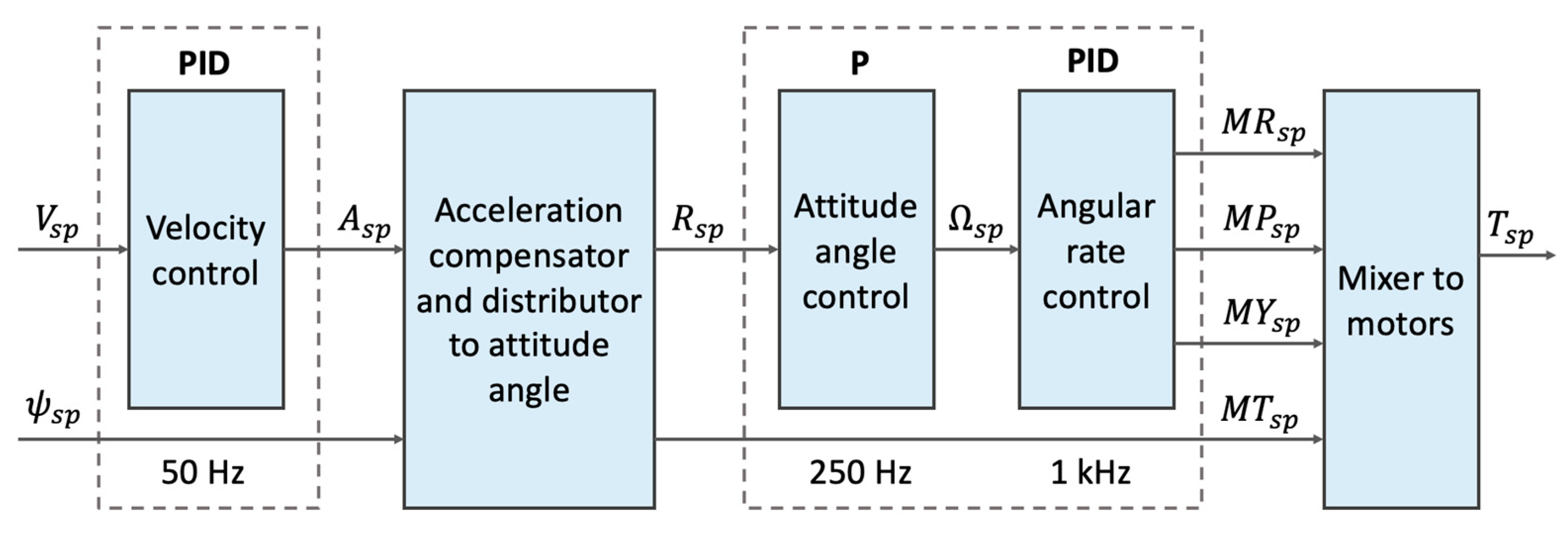
We proposed a cascaded control architecture that combines P and PID controllers with different loop frequencies to achieve a low-level control task. As shown in Figure 6, the velocity setpoint $V_{sp}$ is input to the outer loop velocity control layer, which then outputs the expected acceleration $A_{sp}$ to the compensator and distributor layer. This layer is not a controller but a simple function of $R_{sp}=\mathrm{a}\mathrm{r}\mathrm{c}\mathrm{t}\mathrm{a}\mathrm{n}\left(\frac{A_{sp}}{g}\right)$, where g is the acceleration of gravity, which is a simple decomposition of forces; it will not be further elaborated here. The necessity of this layer is that the thrust of the motors is limited, and our goal is to maximize the maneuverability of drones within the allowed range of power performance. The maximum horizontal acceleration and maximum target attitude angle should be restricted within a reasonable range to avoid crashing due to insufficient power.

Figure 6. Complete cascaded low-level controller combining P and PID controllers in several control layers.

Then, the attitude angle setpoint $R_{sp}$ is input to the cascaded inner loop attitude angle and angular rate controller, which can output the motor thrust in the roll, pitch, and yaw directions, denoted by $M{R}_{sp}$, $M{P}_{sp}$, and $M{Y}_{sp}$, respectively. These three setpoints, along with the throttle setpoint $M{T}_{sp}$, are decomposed into four rotation speed setpoints $T_{sp}$ according to Equation (10):

$$T_{sp}{\left(M1,M2,M3,M4\right)}^T=\left[\begin{array}{cccc}\hfill 1\hfill & \hfill 1\hfill & \hfill -1\hfill & \hfill 1\hfill \\ \hfill 1\hfill & \hfill -1\hfill & \hfill -1\hfill & \hfill -1\hfill \\ \hfill 1\hfill & \hfill -1\hfill & \hfill 1\hfill & \hfill 1\hfill \\ \hfill 1\hfill & \hfill 1\hfill & \hfill 1\hfill & \hfill -1\hfill \end{array}\right]\times \left[\begin{array}{c}{MT}_{sp}\\ {MR}_{sp}\\ {MP}_{sp}\\ {MY}_{sp}\end{array}\right]$$

(10)

Notably, the loop frequency of each controller in cascade control is different. The inner loop controllers for the attitude angle and angular rate operate at 250 and 1 kHz, respectively. This is because the system may respond faster to the angular rate than to the attitude angle. In contrast, the outer loop controller for the velocity operates at 50 Hz. This is because the velocity is indirectly controlled by changing the attitude angle and thus has a slower response.

3.2. High-Level Policy

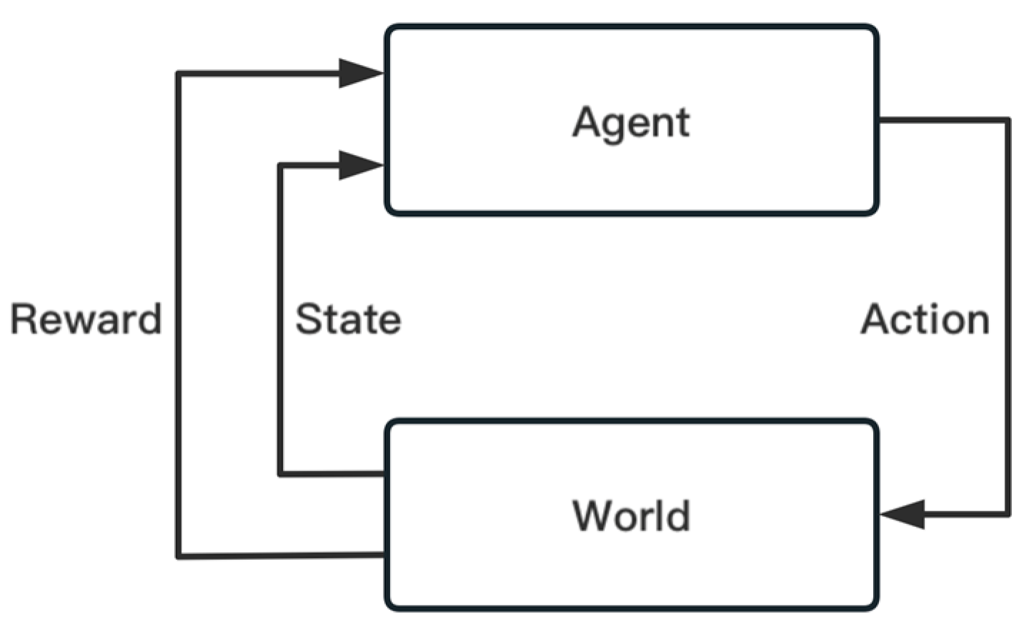
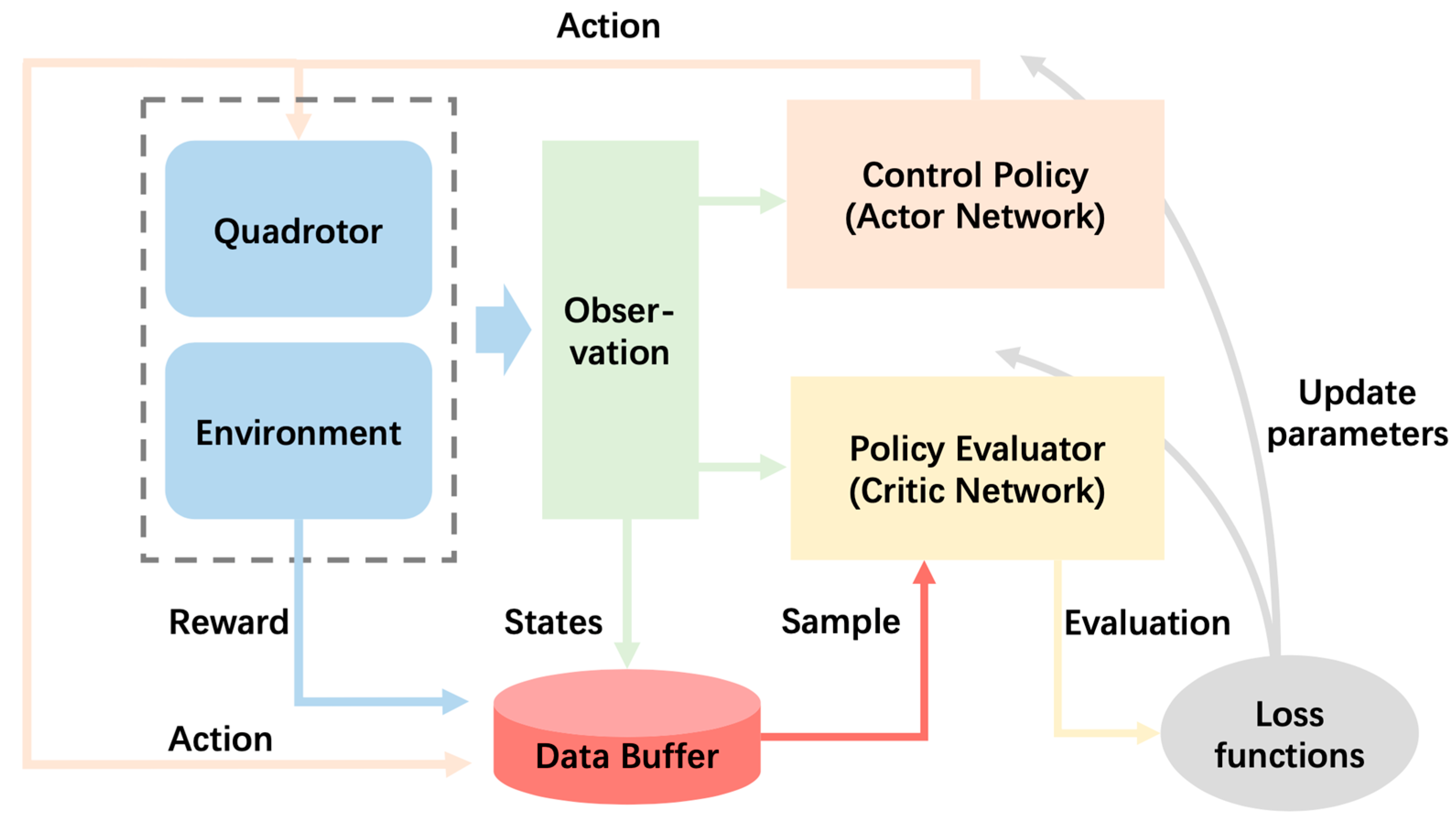
As mentioned previously, we aim to fundamentally solve the issue of high latency in pipelines based on environmental perception through path planning for drones flying in complex environments, which further helps maximize their agile mobility. We utilized the PPO algorithm to handle the information gathered from both onboard and external sensors concerning the environment and drone states in parallel. The algorithm generates control commands that are fed directly to the low-level controller in an end-to-end scheme. The policy training framework is illustrated in Figure 7. The figure shows a partial set of state variables for the drone and its environment, obtained through a combination of onboard and external sensors.

Figure 7. Policy training framework.

The framework consists of two neural networks. The first one is the actor network with parameters $\theta$, which is evaluated to find an approximate optimal control policy, which provides a control command (referred to as an action in RL) to the low-level controller end-to-end based on the observation. At the beginning of the training process, the actions are chosen randomly, the drone transfers to a new state after the actions take effect, and the environment provides a reward that indicates the value of the actions. We refer to each complete navigation task process as an episode, with the sequence of states, actions, and rewards obtained during the process referred to as the trajectory $\tau$. After several episodes, all trajectory data were stored in data buffer $D$, and these data were periodically sampled and used to calculate the value of each state and action based on Equation (1).

Conversely, the value function $V_{\varphi k}$ from Equation (2) reveals the value of a certain state, s, on the $k–\mathrm{t}\mathrm{h}$ iteration, which is obtained through sampling and calculation from the data buffer. The action–value function $Q^{\pi }$ from Equation (3) represents the value of a certain action in that state, which is approximated using a critic network with the parameter $\varphi$. The advantage function representing the advantage of action a in state s can then be obtained as:

$$A^{\pi }\left(s,a\right)=Q^{\pi }\left(s,a\right)-V_{\varphi k}\left(s\right)$$

(11)

For the actor and critic neural networks, we used two different loss functions to calculate the parameter gradients and used stochastic gradient ascent to optimize their performance. The actor network parameters are updated by maximizing the PPO clip objective.

$${\theta }_{k+1}=\mathrm{a}\mathrm{r}\mathrm{g} \underset{\theta }{\mathit{max}}\frac{1}{\left|D_k\right|T}\sum _{\tau \in D_k}\sum _{t=0}^{T}min\left(\frac{{\pi }_{\theta }\left(a_t|s_t\right)}{{\pi }_{{\theta }_k}\left(a_t|s_t\right)}{A}^{{\pi }_{{\theta }_k}}\left(s_t,a_t\right),g\left(ϵ,A^{{\pi }_{{\theta }_k}}\left(s_t,a_t\right)\right)\right)$$

(12)

The set of trajectories collected by applying the control policy ${\pi }_k=\pi \left({\theta }_k\right)$ in the training environment is denoted as $D_k=\left\{{\tau }_i\right\}$. Here, T represents the time step length of a trajectory randomly sampled from $D_k$. Equation (12) shows two surrogate losses, $\frac{{\pi }_{\theta }\left(a_t|s_t\right)}{{\pi }_{{\theta }_k}\left(a_t|s_t\right)}{. A}^{{\pi }_{{\theta }_k}}\left(s_t,a_t\right)$ indicates the step length of parameter updates along the policy gradient, but it will lead to an unexpectedly large update of policy [32]. To ensure a stable and convergent policy optimization, policy updates must be constrained within a reasonable range. The PPO introduced a clip function $g\left(ϵ,A_{{\theta }_k}^{\pi }\left(s_t,a_t\right)\right)$ with a hyperparameter $ϵ$ to limit the step length of policy update:

$$g\left(ϵ,A\right)=\left\{\begin{array}{c}\left(1+ϵ\right)A, A\ge 0\\ \left(1-ϵ\right)A, A<0\end{array}\right.$$

(13)

In contrast to the actor network, the parameter update of the critic network uses a gradient descent, and the objective function is the mean-squared error:

$${\varphi }_{k+1}=\mathrm{a}\mathrm{r}\mathrm{g} \underset{\varphi }{\mathit{min}}\frac{1}{\left|D_k\right|T}\sum _{\tau \in D_k}\sum _{t=0}^T{\left(V_{\varphi }\left(s_t\right)-{\widehat{R}}_t\right)}^2$$

(14)

The ${\widehat{R}}_t$ is the discount accumulated reward from current state $s_t$ to the end of episode, and it can be calculated according to Equation (1) on the trajectory $\tau$, which was sampled from the dataset $D_k$. Here, $V_{\varphi }\left(s_t\right)$ is the evaluation of current state $s_t$ predicted using critic network with current parameters ${\varphi }_k$.

We then obtain the learning algorithm by synchronously optimizing the actor and critic networks stepwise:

3.3. Environment Setting and Reward Function

As shown in Figure 2, there are varying numbers of cylindrical obstacles in the envisioned environments. The goal of this study is to enable drones to traverse cluttered environments safely and quickly. Without any mechanical protection, it may crash after collision with an obstacle. Further, without protective measures, the delicate and sensitive components of a drone, such as its propellers and motors, are vulnerable to damage from collisions with obstacles.

The reward function is the criterion for measuring the quality of a single step of an action, and both the value function $V$ and the action–value function are $Q$ built on this basis. Therefore, the design of reward function must enable the control policy to avoid obstacles and fly to the destination as quickly as possible. Because our learning algorithm uses a clip function and the magnitude of a single policy update is constrained by a hyperparameter $ϵ$, the reward function should be as continuous and smooth as possible in order to ensure stable convergence and avoid local optima. In accordance with these requirements, we designed a composite reward function with five components and their weights $\mathcal{W}$ as follows:

$$r_t=\mathcal{W}\ast \left(\begin{array}{c}\Delta D i s_t\\ E\_Cos{t}_t\\ \left|Over\_speed\right|\\ Symbol\left(collide or arrive\right)\\ Soft\_constrains\end{array}\right)$$

(15)

The first term $\Delta Di{s}_t=Di{s}_{t-1}-Di{s}_t$ is a continuous reward, which presents a positive reward when the drone approaches the goal and a negative reward otherwise, and $Di{s}_t$ is the distance between the drone and the destination. The physical interpretation of the second term, $E\_Cos{t}_t=\left|U_t^2-U_{t-1}^2\right|$, is the energy consumed by the current action. Because the control input $U_t$ is the flight velocity of the drone and $\frac{m{U}^2}{2}$ is the kinetic energy of the drone, we moved the constant parameter $\frac{m}{2}$ into weights for conciseness. This term can reduce meaningless actions, determine the shortest path, and suppress the action noise of a drone during a mission. The third term (Equation (16)) is a soft constraint on the flight speed. In reality, the ability of the drones is restricted due to the performance of their power systems and maneuverability. Long-term high loads may lead to serious accidents such as motor failures, which will provide a negative reward when the drone exceeds the $Max\_speed$, to relieve the burden on the power system.

$$\left|Over\_speed\right|=\left\{\begin{array}{cc}0,& U_t\le Max\_speed\\ \left|U_t-Max\_speed\right|,& U_t>Max\_speed\end{array}\right.$$

(16)

The fourth and final terms were designed to address sparse rewards in specific scenarios. When a drone collides with an obstacle, the symbol function provides a large negative reward as a punishment, whereas reaching the destination provides an extra positive reward. Further, the $Soft\_constrains$ can add points of interest or avoid additional dangerous areas in the task.

4. Experiment

This chapter is divided into four parts to provide a detailed explanation of the experimental results. Section 4.1 showcases the configuration of the simulator environment, in addition to the method and parameters used for policy training. Section 4.2 presents the training results, where the average reward demonstrates the convergence of the algorithm in all the designed environments. Section 4.3 and Section 4.4 describe the performance of the trained controller in a simulator and the real world, respectively. The results indicate that the proposed algorithm performs well in different environments, with both the average and maximum flight speeds surpassing those of the PID algorithm.

4.1. Policy Training Frame in Simulator

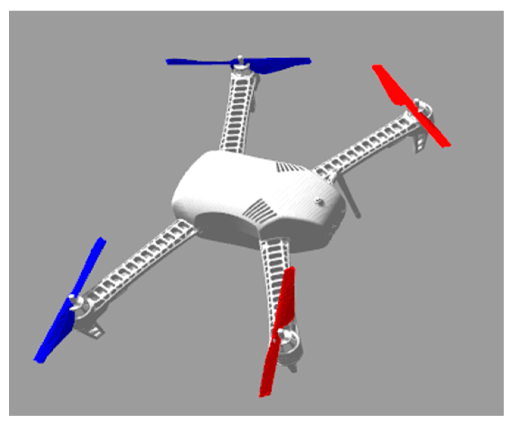
As described in Algorithm 1, the RL training process involves interacting with the environment based on the current policy, accumulating experience data, calculating the advantage function and the gradient of the policy, and updating the parameters of the actor and critic networks—with this process repeated iteratively. To improve the efficiency of collecting the experience data and ensure the safety of the interaction process, we used the Gazebo system to simulate the state of a drone in the real world. We used the model (Figure 8) from [38], which was designed for simulation in a robot operation system (ROS) and Gazebo, whose frame parameters are listed in Table 1.

Algorithm 1 Clipped Advantage Policy Optimization Algorithm.

1: Initialize the actor and critic network using random parameters ${\theta }_0$ and ${\varphi }_0$. 2: Initialize the dataset $D_k$ to store trajectories $\tau$. 3. for k = 0, 1, 2, …, (max episode) do 4. Initialize the environment and drone states, obtain initial observation, set $i$ to 0. 5. for t = 0, 1, 2, …, (max step per episode) do 6.  Get action $a_t$ and log probability $log{a}_t$ of it according to $s_t$ and policy $\pi \left({\theta }_k\right)$. 7.  Implement $a_t$, get new state $s_{t+1}$ and reward $r_t$ from the environment. 8.  Record the tuple $\left(s_t,a_t,r_t,s_{t+1},log{a}_t\right)$ to trajectory $\tau$. 9.  if crashed or arrive the destination or reach max timestep then 10.  Reset the environment and drone states. 11.  Store the trajectory ${\tau }_i$ to $D_k$, $i+1$. 12. end for 13. Calculate rewards-to-go ${\widehat{R}}_t$ using Equation (1) for every trajectory. 14. Calculate the estimation of advantage $\widehat{A}$ according to Equation (11) based on the current value function $V_{{\varphi }_k}$. 15. Update the actor network using Equation (12). 16. Update the critic network using Equation (14). 17. end for

Figure 8. Frame of drone in simulator.

Table 1. Frame parameters of drone model.

Parameter	Value	Unit
Mass	1.5	kg
ixx	0.0347563	kg·m2
iyy	0.0458929	kg·m2
izz	0.0977	kg·m2
Wheel base	0.511	m
Body width	0.47	m
Body height	0.11	m
Mass of rotor	0.005	kg
Length of rotor	0.2	m
Rotor max rotation velocity	838	rad/s
Rotor drag coefficient	1 × 10−6	--

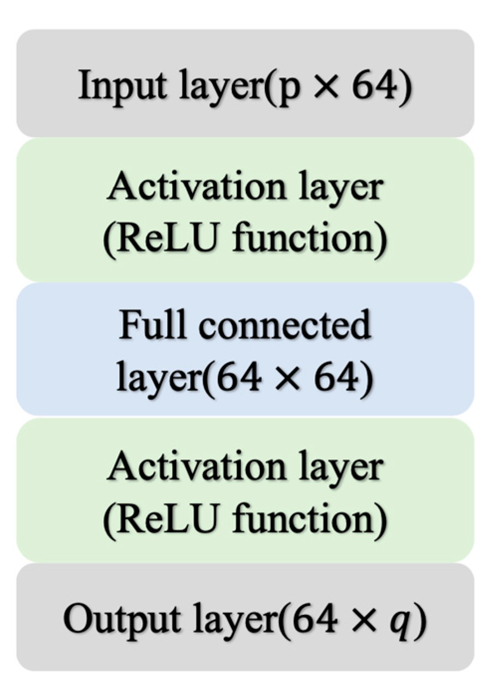
We tackled two structurally identical neural networks as actor and critic networks, which possess the same three-layer network structure and number of parameters, as shown in Figure 9. Both networks use the ReLU function as the activation layer, connected behind the input layer and fully connected layer. The only differences were in the input and output layers. The input layer of both networks has the same dimensions as the system state. However, the output layer of the critic network had q = 1, whereas that of the actor network was q = 2.

Figure 9. Structure of tackled neural networks.

4.2. Policy Training Process

We then used the hyperparameters in Table 2 to train the control policy in all the designed environments. In the experiments, we found that adjusting some of the hyperparameters significantly influenced the training results. For example, an exceptionally small “Max step per episode” will lead to insufficient time for the algorithm to find a complete optimal trajectory, and so more steps are required in a larger scenario. And larger “Timesteps per batch” can improve data utilization efficiency but will also increase data collection time. Our policy optimization algorithm updates the policy, and after each update, the old data become ineffective. Therefore, we chose a parameter value that strikes a balance between efficiency and data collection time. Similar to gradient descent algorithms, the learning rate determines the step size of parameter updates. An excessively small learning rate can lead to slow convergence or becoming stuck in local optima, while an excessively large learning rate can cause oscillations or even divergence. Finally, the “Covariance matrix element value” controls the shape of the action distribution. A larger value will increase the exploration of the policy in the environment, making it less likely to become stuck in local optima. However, it may also slow down the convergence speed of the policy.

Table 2. Hyperparameters of policy training.

Parameter Name	Value
Control period	0.02 s
Max steps	2 × 108
Max step per episode	400
Dimension of states	4
Dimension of actions	2
Timesteps per batch	2048
Discount rate of reward	0.99
Parameter update times per iteration	10
Learning rate	3 × 10−4
$ϵ$ of clip function	0.2
Covariance matrix element value	0.5

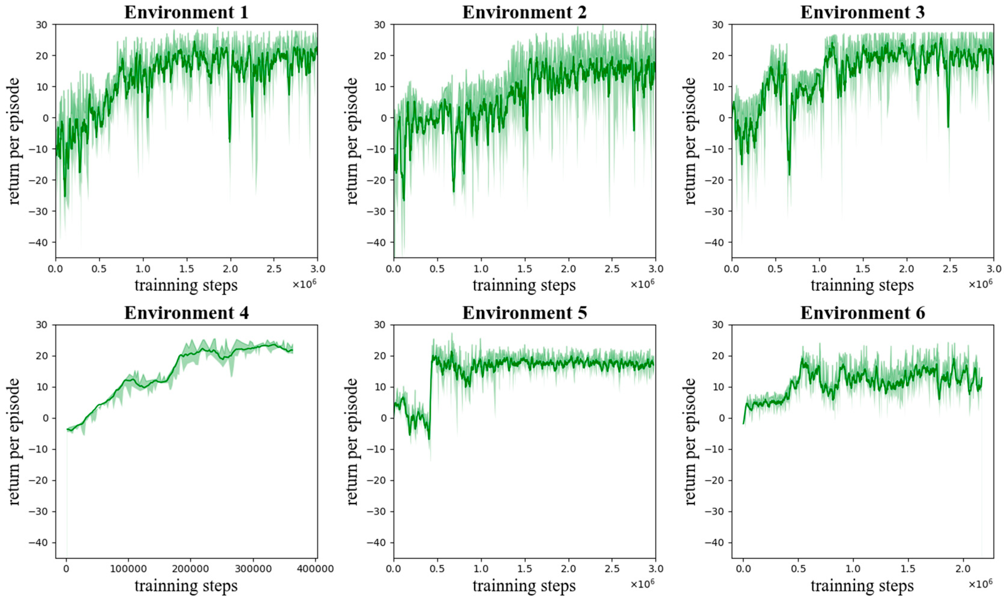
The Gazebo simulator, ROS, and reinforcement learning algorithm were deployed together on a desktop computer running Ubuntu 18.04. The main hardware configuration included an Intel 11,900 k CPU, an Nvidia 3090 GPU, 16-GB RAM, and a 512-GB hard drive. Figure 10 shows the total return for each episode during training and the average of 10 episodes. The y-axis in the figure represents the accumulated reward that is obtained through the policy within an episode, where a higher reward indicates a better performance. Notably, different environments have different upper bounds. As shown in the figure, the proposed algorithm gradually improves the accumulated reward in all environments and finally converges.

Figure 10. Reward during training.

It is worth noting that the training process exhibits different characteristics in environments with different obstacle distribution styles. In environments with more scattered obstacle distributions, such as env 1−3, the training process of the algorithm exhibited higher randomness during convergence. Further, sudden drops in returns may occur over several cycles as the average return increases. This is because the algorithm searches for the optimal policy, and the cluttered environments comprise random obstacles when exploring a certain direction. The returns obtained during these explorations were relatively low, owing to the penalty for collisions in the reward function. After several cycles of optimization, the optimization algorithm finds the optimal policy gradient again, and the average return resumes its upward trend.

In env3, where the obstacles are distributed in an obvious pattern (lined), the exploration–optimization process of the policy is a continuous upward trend. The performance of the algorithm in env5 is impressive. In the initial exploration process, the return value hovers around a low value and even decreases slightly. However, after exploring the gap between the two clusters of obstacles that were designed, the average return quickly rises to near-optimal levels in a few episodes. Similarly, in env6, after exploring the cluster of obstacles, the policy can be quickly optimized to a good level.

In summary, our proposed algorithm demonstrates a strong adaptability to different environments, successfully determines the correct policy gradient, and optimizes the policy to improve the return value in environments with cluttered, uniform, and concentrated obstacle distributions.

4.3. Flight Test in Designed Environments

During the training process of the control policy, because exploration and exploitation must be balanced, actions are sampled from the policy network, and this does not guarantee that the optimal action is always sampled. Therefore, during testing, we designed a simplified structure, as shown in Figure 11, by removing components such as the critic network, loss function, optimizer, and data buffer and retaining only the policy network. Moreover, the control command received by the drone is selected directly based on the output of the policy network, which represents the optimal action. We tested the well-trained policy in all the designed environments in the Gazebo simulator. 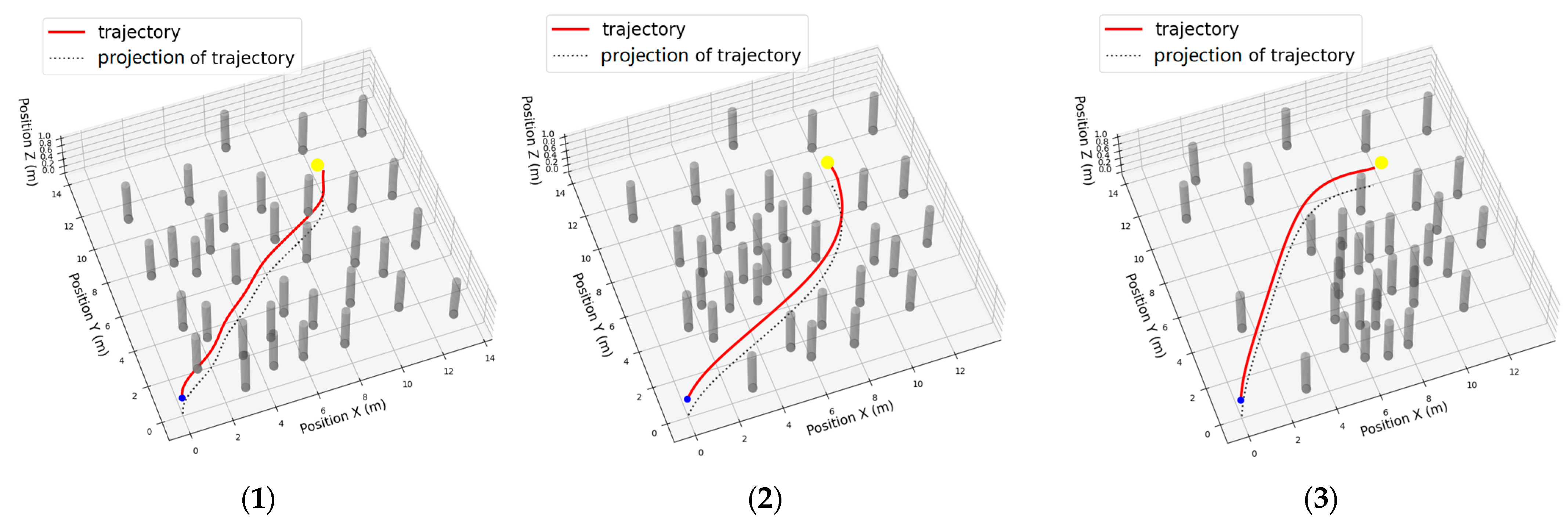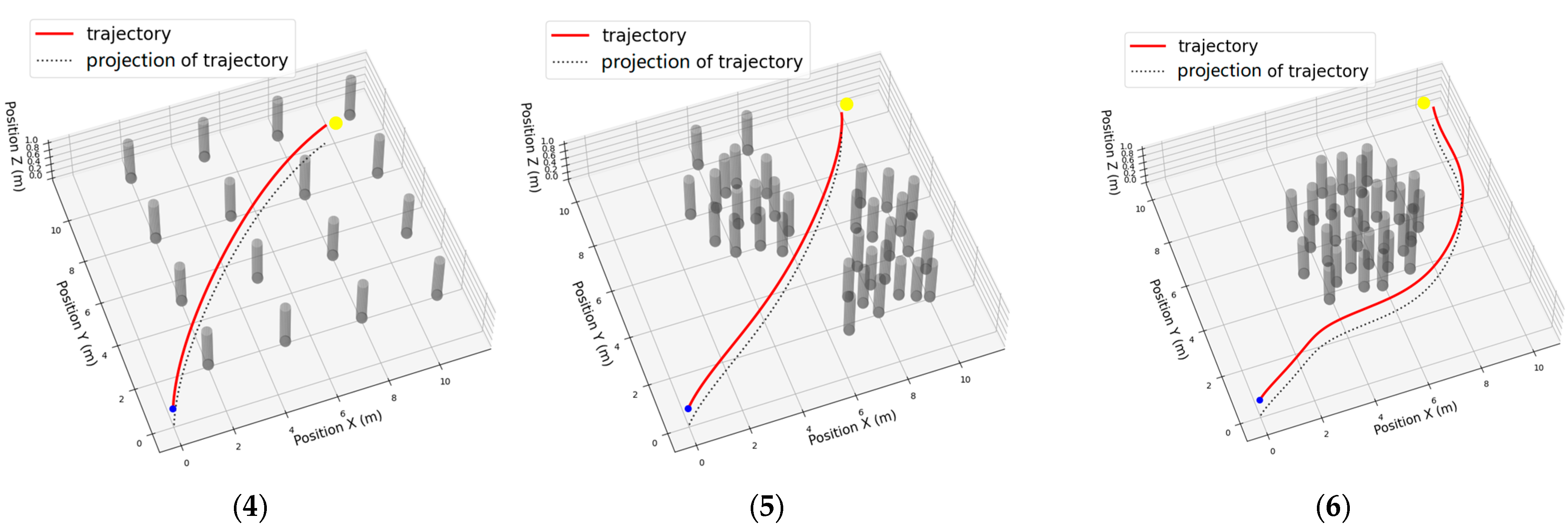Figure 12 shows the flight trajectories and projectories in the X–Y plane.

Figure 11. Test framework.

Figure 12. Test flight trajectory in env (1–6). The mission start from blue dots to yellow boxes.

It can be observed that our algorithm performs well in these scenes and can choose different paths to avoid collisions with obstacles and arrive at the destination as soon as possible. In an environment with randomly distributed obstacles (env 0), neatly arranged obstacles (env 3), and two clusters obstacles (env 4), it selects the paths that are closest to a straight line, perfectly avoiding the obstacles and minimizing the path length. In an environment with a manually designed optimal path, the shortest smooth curve is chosen to minimize energy and time consumption, which proves that the energy evaluation item in our reward function works well. In env 5, with one cluster of obstacles, it first tries to move closer to the direction of the destination and then finds the shortest path to bypass the obstacles.

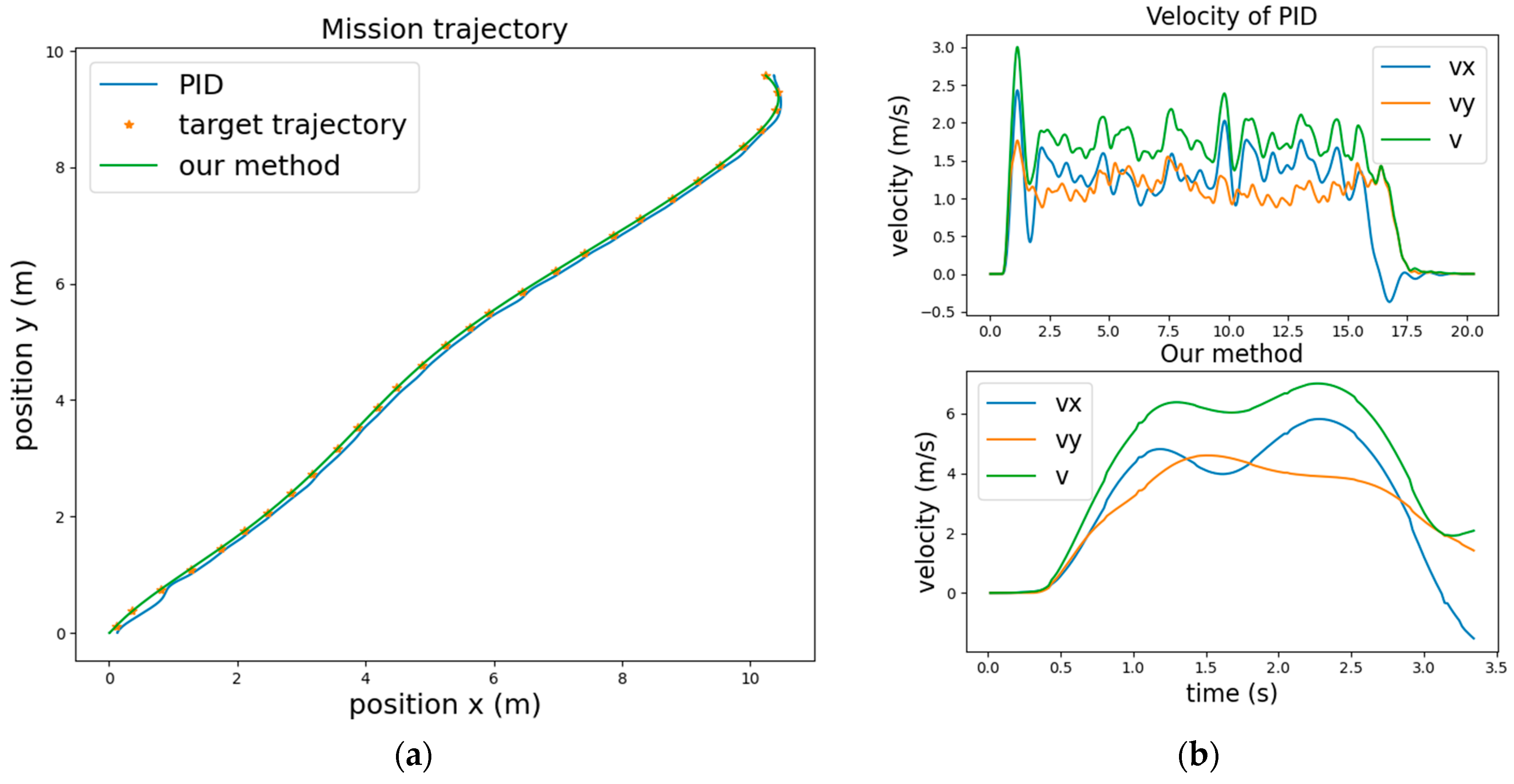
We compared the performance of the proposed method with that of a PID controller, as shown in Figure 13. It was observed that the proposed method achieves a maximum speed of 7 m/s, whereas the PID controller can only reach 3 m/s and maintain it for a short duration. The proposed method completes the task in 3.4 s, while the PID algorithm requires 18 s. This clearly demonstrates that the proposed method has a significant advantage in terms of mission efficiency in complex environments.

Figure 13. Comparison of proposed method with PID. (a) Mission trajectory. (b) Velocity during flight.

4.4. Real-World Test

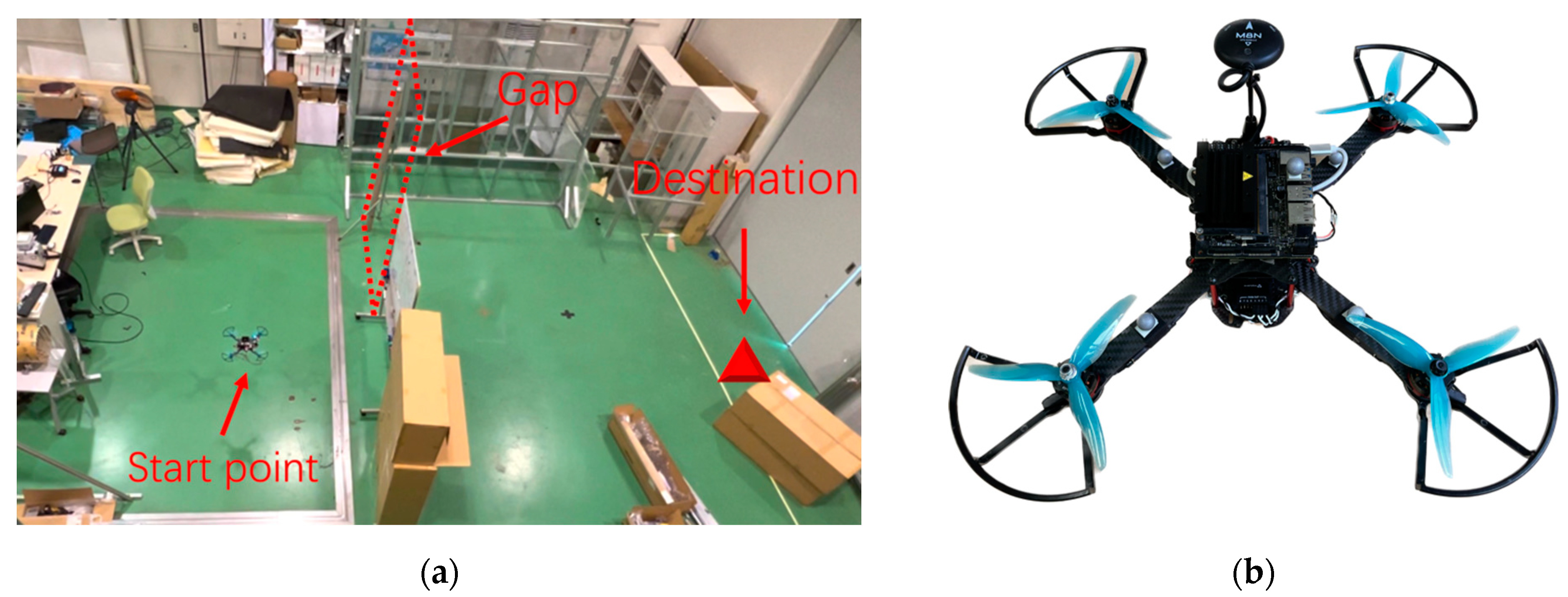
To validate the performance of the proposed algorithm in the real world, we designed a task of navigating through the gap between two walls, as shown in Figure 14a. There is a wall with a gap between the starting point and the destination. The drone must pass through this gap, reach its destination, and hover. The testing methodology is essentially the same as that shown in Figure 11, and the only difference is the substitution of the simulated environment and drone in Gazebo with a real drone (Figure 14b). The low-level controller runs on Pixhawk hardware, whereas our high-level control policy runs on the Jetson Nano. The motion capture system data nodes run in the ROS and communicate through network interfaces.

Figure 14. (a) Real-world environment with walls and gap; (b) drone.

Figure 15a,b show the position and velocity, respectively. For safety purposes, we have implemented a backup system using traditional methods, which can be switched back and forth with the RL method. After 0.2 s from the start of the mission, the control commands generated by the policy begin to take effect, as shown in Figure 15b. Due to the limited area of the site and considering safety, the quadcopter needs to hover after reaching the destination. Therefore, the maximum total speed is only around 4.39 m/s, and in the simulation, it can reach a maximum speed of 10 m/s. This experiment demonstrates that our method can still control the drone to complete the task of navigating through complex environments in the real world, despite the changes in drone hardware and low-level controllers.

Figure 15. (a) Position during mission, start from position (–1, 0), destination position (3, 0); (b) measured velocity and target velocity outputted by well-trained policy during mission.

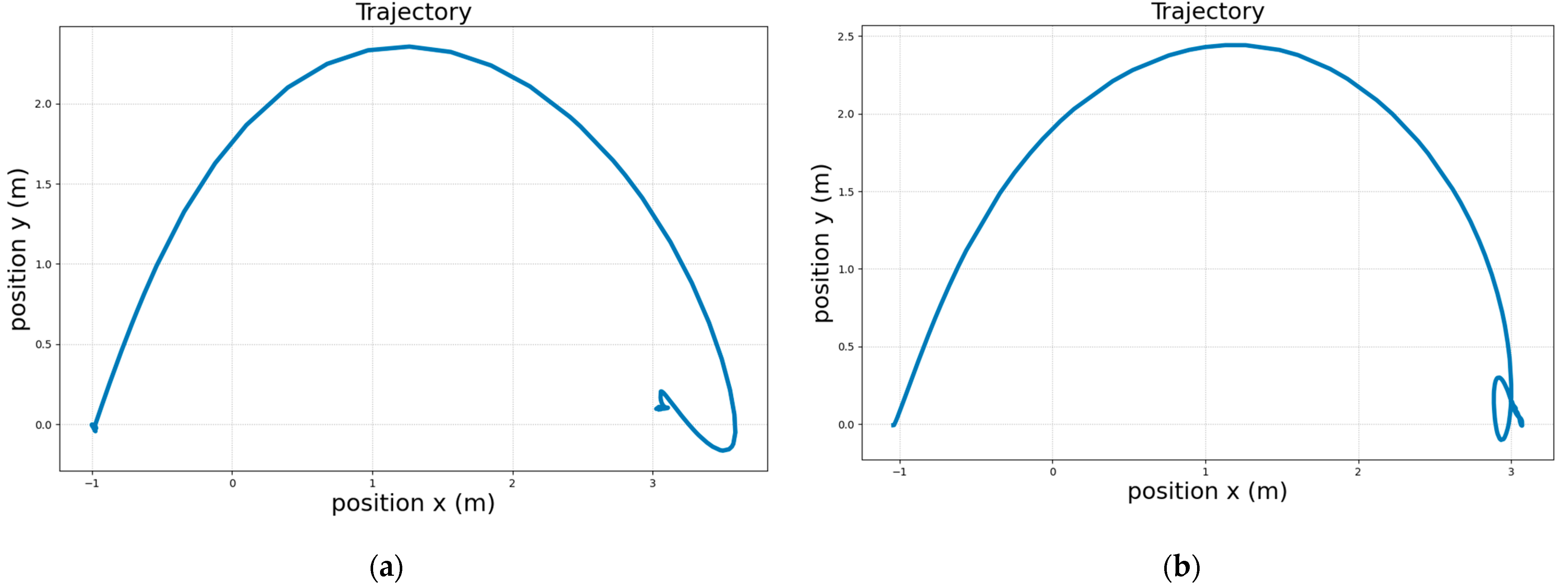
Furthermore, we observed an overshoot that was not present in the simulation tests, as shown in Figure 16a. We analyzed two reasons for this observation. First, the low-level controller of the real-world drone performed poorly than that in the simulator. Second, the policy must wait for all the node data to be updated before it can start the computation. The ROS operates in a soft, real-time manner, and asynchrony between data can cause delays in the control commands. To mitigate the overshoot issue, we adjusted the speed controller parameters and increased the target-tracking speed, which partially improved the situation, as shown in Figure 16b. The test video and code can be found in https://www.youtube.com/watch?v=hRQc1lmJNkY (accessed on 8 July 2023) and https://github.com/pilotliuhx/Drone-navigation-RL.git (accessed on 8 July 2023).

Figure 16. (a) Trajectory before parameter tuning and (b) trajectory after parameter tuning.

5. Conclusions

This paper proposes a novel end-to-end drone control method based on deep reinforcement learning. It directly takes the drone’s state, environmental information, and task objectives as inputs, and outputs the desired velocity to a low-level controller. Compared with traditional model-based pipeline and existing teacher–student learning framework, we faced two main difficulties. The first one was how to lead the policy optimization; we designed a hybrid reward function to evaluate the policy, with a consideration of task progress, energy cost, collision with obstacles, and arrival at the destination. And the other was how to maintain the same level of effectiveness in the simulation within the real world; we used the Gazebo simulator to ensure the reality of physics, and a model-based low-level angular rate, attitude angle, and velocity controller were used to provide consistent performance in velocity command tracking.

To evaluate the performance of the proposed method, obstacle environments with diverse characteristics were designed in a simulator, and the control policy was trained from scratch. Subsequently, the trained control policy was separated and tested in both the Gazebo simulator and a real-world environment. The results show that the proposed method successfully completed flying tasks in complex environments in both simulated and real-world experiments.

It was demonstrated that the proposed method performs well in complex environments with static obstacles. However, certain challenges remain unaddressed. First, the policy’s training efficiency was not high. With our current desktop configuration, a single training session takes approximately 7 h. In future works, we will aim to improve the training efficiency by using parallel training technology. Second, the direct application of the training policy to real-world drones resulted in an overshoot. This discrepancy between the simulation and reality suggests that further adjustments or enhancements may be required to improve the control performance in real-world scenarios.

In addition, there is a potential issue when dealing with moving obstacles. The navigation algorithm must consider the presence of dynamic obstacles and adjust its trajectories accordingly. Further investigation is required to ensure the safe and efficient navigation of drones in the presence of moving obstacles. These challenges provide valuable insights for future research and development, and addressing them will further enhance the performance and applicability of the proposed method.