1. Introduction
Drones, or Unmanned Aerial Vehicles (UAV), have a wide range of uses, from military applications to domestic uses, due to their ease of control, maneuverability, cost-effectiveness, and lack of pilot involvement. Certain drone operations, such as resource exploration and extraction, surveillance, and disaster management, demand autonomous landing as human involvement in these operations may be dangerous, particularly if communication is lost. As a result, recent developments in drone technology have focused on replacing human involvement with autonomous controllers that can make their own decisions.
Launching a drone autonomously is relatively straightforward; the challenging aspect is landing it in a specific location with precision in case of emergency situations. For an autonomous landing to be successful, the drone must have accurate information regarding its landing position, altitude, wind speed, and wind direction. Armed with these data, the UAV can make adjustments to its landing approach, such as reducing speed or altering its altitude, to ensure a safe and successful landing. The landing area can be classified into three categories: static, dynamic, and complex. Static locations are those that are firmly fixed to the ground, such as helipads, airports, and roads. Dynamic locations, on the other hand, are landing areas that are positioned on moving objects, such as a helipad on a ship or drone landing areas on trucks or cars. Complex landing areas are those that have no markings on the surface and can pose a challenge, such as areas near water bodies, hilly regions, rocky terrain, and areas affected by natural disasters such as earthquakes and floods.
Figure 1 gives a view of these types of landing areas.
This work presents a significant contribution in the form of a comprehensive review of how photogrammetry can be applied to static imaging to enhance the accuracy of control decisions in autonomous landing. In addition, the research includes a useful analysis of various landing approaches, including those in static, dynamic, and complex areas. The analysis provides useful information about the possible uses of photogrammetry in combination with a vision-based landing system for accurately locating a target while a UAV lands autonomously. Numerous research endeavors have been dedicated to the topic of UAV autonomous landing, as it presents a range of challenges, including real-time processing, limited resources, high maneuverability requirements, and precise localization difficulties. These challenges will be further discussed in subsequent chapters.
In
Section 2, a literature review is conducted, focusing on the various types of landing systems used in UAVs. This includes a discussion of the Electromagnetically Guided Landing System, Inertial Navigation System, and Vision-Based Landing System.
Section 3 explores the different types of landing areas, including Static Landing Areas, Dynamic Landing Areas, and Complex Landing areas. In
Section 4, the focus shifts to landing on extra-terrestrial bodies, with a discussion of Pose Estimation Techniques and Object Classification.
Section 5 is dedicated to the topic of finding the altitude of the image, with a discussion of Structure from Motion and Photogrammetry. The latter is further divided into four subcategories: Nadir Photogrammetry, Convergent Photogrammetry, Low Oblique Photogrammetry, and High Oblique Photogrammetry.
Section 6 presents the preliminary work and results of the study, with a discussion of the performance of standard filters and feature-matching techniques. Finally, the study is wrapped up in
Section 7, which presents a summary of the main discoveries, addresses the study’s constraints, and offers suggestions for potential research endeavors.
2. Literature Review
The development of unmanned aerial vehicle technology dates back to ancient times. In fact, the concept of UAVs existed before the invention of manned flight. According to Chinese historical records, around 200 AD, the Chinese attached oil lights to paper balloons to warm the air and make the balloons float. As the balloons hovered above their rivals at night, the enemy troops were frightened and believed that a divine force was behind the flight, and this incident marks the first recorded flight in human history. In the late 90s, the British tested a radio-controlled aircraft from the First World War called “The Aerial Target” in March 1917, which marked the first recorded instance of a drone flying under controlled conditions [
1]. Following this breakthrough, UAV technology experienced rapid growth. As the technology reached its saturation point within a few decades, researchers shifted their focus from developing various types of UAVs to autonomous flight. Autonomous landing plays a critical role in autonomous flight and, to this day, research on autonomous landing continues to progress and evolve the field of UAV technology. The pre-existing system for the landing process of a drone is next discussed.
2.1. Electromagnetically Guided Landing System
Electromagnetically Guided Landing Systems rely on the use of electromagnetic fields to guide aircraft during the approach and landing phase. These fields are generated by ground-based transmitters and received by antennas on the aircraft. The system provides precise information about the aircraft’s position, altitude, and velocity, allowing for highly accurate guidance during the landing phase. There are several types of electromagnetically guided landing systems, including Local Area Augmentation Systems (LAAS), Global Navigation Satellite System Landing Systems (GLS), Pulsed Localizers, and Millimeter-Wave Landing Systems (MWLS). Each system has its own unique advantages and disadvantages, and the choice of system will depend on factors such as the airport location, aircraft type, and operational requirements.
2.2. Inertial Navigation Systems
The Inertial Navigation System (INS) is a self-sufficient navigation mechanism that employs gyroscopes and accelerometers to monitor the three-dimensional motion of an aircraft. The accelerometers measure the aircraft’s acceleration, while the gyroscopes measure the rate of change in the aircraft’s orientation. These data are integrated over time to determine the aircraft’s velocity and position relative to its starting point. INS is typically classified into two types: strap-down INS and gimballed INS. Strapdown INS is a more modern, lightweight design that directly measures the acceleration and angular velocity of the aircraft, while gimballed INS uses a rotating platform to maintain a stable orientation. Despite their high accuracy, INS has some limitations, including errors caused by sensor drift over time and the need for periodic calibration. INS is widely used in aviation, particularly in navigation, flight control systems, and landing systems. Its ability to provide accurate and reliable navigation information makes it an essential tool for pilots and aircraft manufacturers.
2.3. Vision-Based Landing System
Vision-based landing systems are a popular approach to autonomous landing that rely on cameras and computer vision algorithms to detect and recognize landmarks on the ground. The system acquires images of the landing region and proceeds to extract features from them, which are then utilized to identify the landing area. The extracted features consist of high-level visual attributes such as texture, edges, corners, and patterns, as well as low-level features such as colour and brightness. After the feature extraction, the system matches the features against a pre-existing database of features to recognize the landing area. While vision-based landing systems can be highly effective, they require sophisticated algorithms and powerful processing hardware to operate in real-time. Researchers are constantly developing faster and more efficient approaches to improve the speed and accuracy of these systems. Despite their effectiveness, these methods take a long time to extract objects and localize them, which leads the researchers to develop faster and more efficient approaches.
Several techniques and tools have been created for object identification and localization in images. The following list highlights some of the frequently utilized approaches: Iiyama et al. [
2] utilized reinforcement learning to localize the object, which involves intercepting the map obtained from techniques such as Digital Elevation Model (DEM) and Light Detection and Ranging (LiDAR) using an auto-encoder. Meanwhile, Skinner et al. [
3] utilized the Uncertainty Aware Learning Bayesian and SegNet techniques to enhance the precision of the pixels selected for the landing site. This was achieved by integrating network uncertainty into the final safety map, resulting in the optimal output. Similarly, Minghui et al. [
4] used BboxLocate Net, Kalman filter estimator, and Point Refine Net for object classification and target localization. BboxLocate Net is a network designed to recognize the bounding boxes of a target and obtain its coordinates. The data obtained from this process can be used in conjunction with the extended Kalman filter to improve the precision of spatial localization. Finally, PointRefine Net is utilized to further enhance decision accuracy. Moreover, in their study, Yu et al. (2018) [
5] employed various computer vision components such as DTM, DEM, DSM, and PSPNet network layers in combination with a MobileNet V2 base feature extractor to detect and localize objects. The authors also utilized YOLO V2 for identifying potential landing areas.
In their study, Bickel et al. (2021) [
6] utilized three different methods—HORUS, DestripeNet, and PhotonNet—for object localization and classification. HORUS employs a physical noise model of the Narrow Angle Camera and environmental data to eliminate noise from the CCD and phone noise. The process involves using two deep neural networks sequentially to extract features and enhance data accuracy. Meanwhile, in the study by Ciabatti et al. (2021) [
7], the classification task was achieved using Deep Reinforcement Learning and Transform Learning, specifically DDPG. Using the Bullet/PyBullet library, the authors developed a physical environment in which they defined a lander via the standard ROS/URDF framework. They utilized 3D terrain models obtained from official NASA 3D meshes from different missions to add realism to the simulation. An outline of the current approach for object classification and localization is provided in
Table 1.
Aside from the approaches mentioned earlier, there are other algorithms available for the purpose of classification and localization. Various research studies have delved into several deep learning techniques, such as Edge Detection, Alex Net, ERU Net, YOLO, DPM, R-CNN, Over Feet, U-Net, and Structured Random Forest [
8,
9,
10,
11,
12,
13,
14,
15,
16]. Unsupervised Learning techniques such as Hough Transformation and its enhanced algorithm, Genetic Algorithms, Hough Transformation and Radial Consistency approach, Template Matching, and Morphological Image Processing have been discussed [
17,
18,
19,
20,
21]. Kang et al. (2018) [
22], Xin et al. (2017) [
23], and Urbach et al. (2009) [
24] introduced several Supervised Learning techniques for object classification and localization, which include Support Vector Machine, Ada Boost, and Notation of Looking for Perspective. The KLT detector discussed in [
25] employs a combined approach of Supervised and Unsupervised Learning, while Template Matching, which is a combination of Supervised and Deep Learning approaches, was discussed in [
26].
3. Type of Landing Areas
The categorization of target locations is divided into three types: Static, Dynamic, and Complex, with Static locations further subdivided into cooperative target-based, and Dynamic locations being classified into vehicle-based and ship-based locations. Xin et al. [
27] discuss cooperative target-based autonomous landing, which is further classified into classical machine learning solutions such as Hough transformation, template matching, Edge detection, line mapping, and sliding window approaches. The author begins with basic clustering algorithms and progresses through deep learning algorithms to address the static location.
Cooperative-based landing pertains to landing sites that are clearly defined and labeled with identifiable patterns, such as the letter “T” or “H”, a circle, a rectangle, or a combination of these shapes, based on specific geometric principles, as described in Xin (2022) [
27]. The different types of landing area markings are depicted in
Figure 2.
3.1. Static Landing Area
The localization of different types of markings relies on a range of techniques, from image processing to advanced machine learning. Localization of the “T” marking helipad achieves the maximum precision at specific poses using Canny Edge detection, Hough Transform, Hu invariant, Affine moments, and adaptive threshold selection [
28,
29]. Localization of the “H” marking achieves a success rate of 97.3% using image segmentation, depth-first search, and adaptive threshold selection in [
30], while it achieves the maximum precision at pose 0.56
using image extraction and Zernike moments obtained in [
31].
The “Circle” marking’s localization is addressed in two studies, namely [
32,
33]. Through the implementation of solvePnPRansac and Kalman filters, Benini et al. [
32] were able to achieve a position error that is less than 8% of the diameter of the landing area, while maximum precision at pose 0.08
using an Extended Kalman filter was achieved by [
33]. Detecting combined marking types is discussed in [
34,
35,
36,
37]. The maximum precision at specific poses using template matching, Kalman filter, and a profile-checker algorithm was achieved in [
34]. Meanwhile, the other combined detection method predicts the maximum precision at pose 0.5
using tag boundary segmentation, image gradients, and adaptive threshold [
35]. Ref. [
36] achieves maximum precision at a position of less than 10 cm using Canny Edge detection, adaptive thresholding, and Levenberg–Marquardt. Lastly, the final combined detection approach obtains maximum precision at a position of less than 1% using HOG, NCC, and AprilTags [
37].
Forster et al. [
38] designed a system to detect and track a target mounted on the vehicle using computer vision algorithms and hardware. The system used in the Mohamed Bin Zayed International Robotics Challenge 2017 (MBZIRC) employed a precise RTK-DGPS to determine the target location, followed by a circle Hough transform to accurately detect the center of the target. By tracking the target, the UAV adjusted its trajectory to match the movement of the vehicle. The system successfully met the requirements of the task and was ranked as the best solution, considering various constraints. There are some limitations in the system, such as weather conditions and vehicle speed, which may affect its performance. Overall, this paper provides an interesting approach to solving an important problem in robotics research, which has potential applications in various fields such as aerial monitoring and humanitarian demining operations. An overview of the algorithms available for static landing site detection based on landing marking shape is presented in
Table 2.
3.2. Dynamic Landing Area
Two categories of dynamic landing areas exist based on the motion of the platform, namely ship-based and vehicle-based landings. Due to the complexity of landing on a moving platform, LiDAR sensors are used in conjunction with computer vision techniques. The landing process is facilitated using a model predictive feedback linear Kalman filter, resulting in a landing time of 25 s and a position error of less than 10 cm [
39]. Another algorithm uses nonlinear controllers, state estimation, convolutional neural network (CNN), and velocity observer to achieve maximum precision at positions less than (10, 10) cm [
40], while the algorithm employs a deep deterministic policy gradient with Gazebo-based reinforcement learning and achieves a landing time of 17.5 s with a position error of less than 6 cm [
41]. Lastly, the algorithm proposed in [
42] uses extended Kalman, extended H∞, perspective-n-point (PnP), and visual–inertial data fusion to achieve maximum precision at positions less than 13 cm.
The algorithm presented in [
43] utilizes extended Kalman and visual–inertial data fusion techniques to achieve a landing time of 40 s for ship-based landing area detection. Meanwhile, another algorithm employs a Kalman filter, artificial neural network (ANN), feature matching, and Hu moments to achieve a position error of (4.33, 1.42) cm [
44]. The approach outlined in [
45] utilizes the EPnP algorithm and a Kalman filter, but no experimental results are presented. Battiato et al. [
46] have introduced a system that enables real-time 3D terrain reconstruction and detection of landing spots for micro aerial vehicles. The system is designed to run on an onboard smartphone processor and uses only a single down-looking camera and an inertial measurement unit. A probabilistic two-dimensional elevation map, centered around the robot, is generated and continuously updated at a rate of 1 Hz using probabilistic depth maps computed from multiple monocular views. This mapping framework is shown to be useful for the autonomous navigation of micro aerial vehicles, as demonstrated through successful fully autonomous landing. The proposed system is efficient in terms of resources, computation, and the accumulation of measurements from different observations. It is also less susceptible to drifting pose estimates. An overview of the current dynamic landing methods is given in
Table 3, which calls for more sophisticated algorithms because of how complicated the moving platform is.
3.3. Complex Landing Area
The complex landing area is a challenging task for autonomous landing systems. The terrain in these areas can have various obstacles and hazards, and it is not always possible to find a suitable landing area. Researchers have explored different methods for identifying safe landing areas in complex terrain, but the research in this area is limited. Fitzgerald and Mejia’s research on a UAV critical landing place selection system is one such effort [
43,
44]. To locate a good landing spot, a monocular camera and a digital elevation model (DEM) are used. This system has multiple stages, including primary landing location selection, candidate landing area identification, DEM flatness analysis, and decision-making. The method’s limitations stemmed from the fact that it only used the Canny operator to remove edges and that the flat estimation stage’s DEM computation lacked resilience.
Research on unstructured emergency autonomous UAV landings using SLAM was conducted during the year 2018, where the use of DEM and LiDAR in their approach are evaluated and their advantages and limitations are discussed [
47]. The research was conducted by using monocular vision SLAM and a point cloud map to identify the UAV and split the grid into different heights to locate a safe landing zone. After denoising and filtering the map using a mid-pass filter and 3D attributes, the landing process lasted 52 s, starting at a height of 20 m. The experimental validation was conducted in challenging environments, demonstrating the system’s adaptability. In order to fulfill the demands of a self-governing landing, the sparse point cloud was partitioned based on different elevations. Furthermore, Lin et al. [
48] deliberated landing scenarios in low illumination settings.
To account for the constantly changing terrain in complex landing areas, it is advisable to identify multiple suitable landing sites to ensure the safety of the UAV. Once landing coordinates have been identified, the optimal landing spot and approach path should be determined. Cui, et al. [
49] proposed a way that calculates the landing area’s criteria based on energy consumption, the safety of the terrain, and the craft’s performance. A clearer comprehension of landing point selection is provided in
Figure 3, which displays the identification of two landing targets—Target A and Target B—along with the corresponding trajectories to reach them. It is advisable to determine the shortest trajectory to the alternative target in the event of a last-minute change.
4. Landing on Extra-Terrestrial Bodies
For the above-said problem, we can also consider adopting the landing approach utilized by spacecraft on other extra-terrestrial bodies [
50]. Precise Landing and Hazard Avoidance (PL&HA) [
51,
52,
53,
54,
55,
56] and the Safe and Precise Landing Integrated Capabilities Evolution (SPLICE) are two projects that NASA has been working on [
57]. Moreover, NASA is working on a project called ALHAT, which stands for Autonomous Landing Hazard Avoidance Technology [
58,
59,
60,
61,
62,
63,
64,
65,
66,
67,
68]. However, a significant limitation of ALHAT is that it relies solely on static information such as slopes and roughness to select a landing area, making the maneuvering of the craft more challenging. S.R. Ploen et al. [
69] proposed an algorithm that uses Bayesian networks to calculate approximate landing footprints and make it feasible. Researchers are currently working on similar aspects. In that case, the classical method of object classification can be employed to simplify the process of identifying objects in space. However, prior to delving into object classification, it is essential to determine the angle and pose of the spacecraft for greater accuracy. Subsequently, the article will delve into pose estimation techniques followed by object classification techniques.
4.1. Pose Estimation Techniques
Determining the spacecraft’s pose requires an estimation based on the camera’s angle with respect to the ground view. Deep learning models are mainly used for pose estimation. The previously available pose estimation techniques are studied by Uma et al. [
70], which has been summarized as follows.
In their respective studies, Sharma et al. (2018) [
71], Harvard et al. (2020) [
72], and Proencca et al. (2020) [
73] employed different techniques to analyze the PRISMA dataset. Sharma et al. [
71] utilized the Sobel operator, the Hough transform, and a WGW approach to detect features of the target, regardless of their size. On the other hand, Harvard et al. [
72] utilized landmark locations as key point detectors to address the challenge of high relative dynamics between the object and the camera. They also employed the 2010 ImageNet ILSVRC dataset in their approach. A deep learning framework that utilizes soft classification and orientation and outperformed straightforward regression is presented by Proencca et al. [
73]. The Dataset used in the study was the URSO, an Unreal Engine 4 simulator. According to Sharma et al. (2018) [
74], their approach demonstrated higher feature identification accuracy compared to traditional methods, even when dealing with high levels of Gaussian white noise in the images. The SA-LMPE method used by Chen et al. [
75] improves posture refinement and removes erroneous predictions, while the HRNet model correctly predicted two-dimensional landmarks, using the SPEED Dataset. Zeng et al. (2017) [
76] utilized deep learning methods to identify and efficiently represent significant features from a simulated space target dataset generated by the Systems Tool Kit (STK). Wu et al. (2019) [
77] used a T-SCNN model trained on images from a public database to successfully identify and detect space targets in deep space photos. Finally, Tao et al. (2018) [
78] used a DCNN model trained on the Apollo spacecraft simulation Dataset from TERRIER, which showed resistance to variations in brightness, rotation, and reflections, as well as efficacy in learning and detecting high-level characteristics.
4.2. Object Classification
The objects of interest in this scenario are craters and boulders found on a particular extraterrestrial body. A crater is a concave structure that typically forms as a result of a meteoroid, asteroid, or comet’s impact on a planet or moon’s surface. Craters can vary greatly in size, ranging from small to very large. Conversely, a boulder is a large rock that usually has a diameter exceeding 25 cm. The emergence of boulders on the surfaces of planets, moons, and asteroids can be attributed to several factors including impact events, volcanic activity, and erosion.
4.2.1. Deep-Learning Approach
Once the spacecraft’s pose has been determined, the objective is to land the spacecraft safely by avoiding craters and boulders. To achieve this objective, several algorithms have been developed. Li et al. (2021) [
8] suggest a novel approach to detect and classify planetary craters using deep learning. The approach involves three main steps: extracting candidate regions, detecting edges, and recognizing craters. The first stage of the proposed method involves extracting candidate regions that are likely to contain craters, which is done using a structure random forest algorithm. In the second stage: the edge detection stage, the edges of craters are extracted from the candidate regions through the application of morphological techniques. Lastly, in the recognition stage, the extracted features are classified as craters or non-craters using a deep learning model based on the AlexNet architecture. Wang, Song et al. [
9] propose a new architecture called “ERU-Net” (Effective Residual U-Net) for lunar crater recognition. ERU-Net is an improvement over the standard U-Net architecture, which is commonly used in image segmentation tasks. The ERU-Net architecture employs residual connections between its encoder and decoder blocks, along with an attention mechanism that aids the network in prioritizing significant features while being trained.
4.2.2. Supervised Learning Approach
Supervised detection approaches utilize machine learning techniques and a labeled training dataset in the relevant domain to create classifiers, such as neural networks (Li & Hsu, 2020) [
79], support vector machines (Kang et al., 2019) [
22], and the AdaBoost method (Xin et al., 2017) [
23]. Kang et al. (2018) [
22] presented a method for automatically detecting small-scale impact craters from charge-coupled device (CCD) images using a coarse-to-fine resolution approach. The proposed method involves two stages. Firstly, large-scale craters are extracted as samples from Chang’E-1 images with a spatial resolution of 120 m. Then, the histogram of oriented gradient (HOG) features and a support vector machine (SVM) classifier are used to establish the criteria for distinguishing craters and non-craters. Finally, the established criteria are used to extract small-scale craters from higher-resolution Chang’E-2 CCD images with spatial resolutions of 1.4 m, 7 m, and 50 m. Apart from that Xin et al. [
23] propose an automated approach to identify fresh impact sites on the Martian surface using images captured by the High-Resolution Imaging Science Experiment (HiRISE) camera aboard the Mars Reconnaissance Orbiter. The method being proposed comprises three primary stages: the pre-processing of the HiRISE images, the detection of potential impact sites, and the validation of the detected sites using the AdaBoost method. The potential impact sites are detected using a machine-learning-based approach that uses multiple features, such as intensity, texture, and shape information. The validation of the detected sites is done by comparing them with a database of known impact sites on Mars.
An automated approach for detecting small craters with diameters less than 1 km on planetary surfaces using high-resolution images is presented by Urbach and Stepinski [
24]. The three primary stages of the suggested technique include pre-processing, candidate selection, and crater recognition, with the pre-processing stage transforming the input image to improve features and minimize noise. In the candidate selection step, a Gaussian filter and adaptive thresholding are used to detect potential crater candidates. In the crater recognition step, a shape-based method is employed to differentiate between craters and non-craters. It is shown that the suggested technique works well for finding tiny craters on the Moon and Mars.
4.2.3. Unsupervised Learning Approach
The unsupervised detection approach utilizes image processing and target identification theories to identify craters by estimating their boundaries based on the circular or elliptical properties of the image [
80]. The Hough transform and its improved algorithms (Emami et al., 2019) [
17], the genetic algorithm (Hong et al., 2012) [
18], the radial consistency approach (Earl et al., 2005) [
19], and the template matching method (Cadogan, 2020; Lee et al., 2020) [
20] are among the common techniques utilized for this method. The morphological image processing-based approach for identifying craters involves three primary steps: firstly, the morphological method is used to identify candidate regions, followed by the removal of noise to pinpoint potential crater areas; secondly, fast Fourier transform-based template matching is used to establish the association between candidate regions and templates; and finally, a probability analysis is utilized to identify the crater areas [
21]. The advantage of the unsupervised approach is that it can train an accurate classifier without requiring the labeling of a sizable number of samples. This strategy can be used when an autonomous navigation system’s processing power is constrained. Nevertheless, it struggles to recognize challenging terrain.
4.2.4. Combined Learning Approach
To detect craters, a combined detection methodology employs both unsupervised and supervised detection methods. For example, consider the KLT detector, which is a combination detection technique, to extract probable crater regions [
25]. In this approach, supervised detection methodology was used, and image blocks were used as inputs, while the detection accuracy was significantly influenced by the KLT detector’s parameters. Li and Hsu’s (2020) [
26] study employed template matching and neural networks for crater identification. However, this approach has the drawback of being unable to significantly decrease the number of craters in rocky areas, leading to weak crater recognition in mountainous regions. Li et al. [
8] propose a three-stage approach for combined crater detection and recognition. In the first stage, a structured random forest algorithm is utilized for extracting the crater edges. The second stage involves candidate area determination through edge detection techniques based on morphological methods. The third stage involves the recognition of candidate regions using the AlexNet deep learning model. Experimental results demonstrate that the recommended crater edge detection technique outperforms other edge detection methods. Additionally, the proposed approach shows relatively high detection accuracy and accurate detection rate when compared to other crater detection approaches.
5. Finding the Altitude from an Image
Once the landing area is identified along with the pose of the vehicle, the altitude of the drone can be calculated. It can be done by using sensors or by using computer vision techniques. The sensors such as altimeter, LiDAR, or RADAR can be used to find the altitude of the drone. Another way to calculate the altitude is by computer vision techniques [
81]. In order to apply computer vision techniques, the height of the object in the image needs to be known, which can be determined using methods such as Structure from Motion (SFM) and Photogrammetry.
5.1. Structure from Motion Methods
The method known as Structure from Motion (SFM) analyzes the motion of an object in a scene to estimate its 3D structure from a 2D image [
82]. To calculate the height, at least two images of the object captured from distinct viewpoints are necessary. By examining changes in object position between two images, SFM can ascertain its relative location in 3D space, including height. This approach demands a significant amount of computational power and a solid grasp of computer vision and 3D geometry.
Figure 4 gives a pictorial representation of the Structure from Motion Model.
5.2. Photogrammetry
Photogrammetry refers to a technique of obtaining measurements by analyzing the appearance of an object in photographs and taking into consideration various camera parameters such as size and focal length. By doing this, it is feasible to calculate the object’s height from the photograph [
83]. Several factors affect the accuracy of photogrammetry, including image quality, object location within the image, and camera parameters such as focal length, position, orientation, and lens distortion. The camera’s focal length, which is the distance between the camera sensor and the lens, can vary depending on the camera type. For example, a regular camera has a focal length of approximately 30 mm, while a camera with a wide-angle lens has a focal length of around 152 mm. In contrast, a camera with a super wide-angle lens typically has a focal length of 88 mm, and the focal length of a mobile phone camera is usually greater than 300 mm. The brief methods of camera calibration were studied by Roncella et al. in [
84].
Figure 5 gives an elaborate view of image formation in a digital camera. Photogrammetry uses accurate 2D maps and elevation models of the environment, which can be useful for the navigation and localization of the UAVs. There are four types of photogrammetry used for drones, which will be discussed next.
5.2.1. Nadir Photogrammetry
Nadir Photogrammetry is a method of photogrammetry that involves capturing aerial images of an object or area from directly overhead, typically from a camera mounted on a drone or an aircraft [
85]. The term “nadir” refers to the point directly beneath the camera lens, which is usually the highest point of the object or area being photographed.
5.2.2. Convergent Photogrammetry
Convergent photogrammetry is a method of photogrammetry that involves capturing multiple images of an object or scene from different positions and angles to create a 3D model. The term “convergent” denotes that the optical axes of the camera lenses employed to capture images meet at a single point, usually at the center of the object or scene under scrutiny [
86]. Both Nadir and Convergent photogrammetry are commonly used in a variety of applications, including surveying, mapping, architecture, and industrial design. They have the ability to create precise and elaborate 3D models of objects and surroundings, providing valuable aid in visualization, analysis, and design applications [
87].
5.2.3. Low Oblique Photogrammetry
Low oblique refers to a specific type of aerial photography or photogrammetry in which images of an object or area are taken from an aerial viewpoint that is slightly tilted or inclined [
47]. Low oblique photography involves mounting the camera at an angle ranging from around 30 to 60 degrees away from the vertical axis. Compared to high oblique photography, in which the camera is tilted at a steeper angle, low oblique photography captures more of the horizon and background, providing additional context to the object or area being photographed. However, low oblique photography can also introduce more distortion and parallax errors compared to nadir photography, which may require additional processing or corrections to achieve accurate results.
5.2.4. High Oblique Photogrammetry
Similar to low oblique photography, high oblique images are captured by mounting the camera at an angle away from the vertical axis. However, in high oblique photography, the camera is typically positioned at an angle greater than 60 degrees [
88]. Compared to low oblique photography, in which the camera is tilted at a shallower angle, high oblique photography captures less of the horizon and background, but provides a more detailed view of the object or area being photographed. However, high oblique photography can introduce more distortion and parallax errors compared to nadir photography, which may require additional processing or corrections to achieve accurate results.
Once the size of the object, which is our reference present in the image, is known, then from that the altitude of the drone can be measured. To measure the altitude, there are some constraints to be satisfied. Firstly, the image taken should be a non-cropped one and must be as flat as possible. While taking the picture, the lens plane must be parallel to the ground plane, which will help to minimize the distortions and ensure accurate measurements of elevation. Secondly, the line to measure must be parallel to one of the edges of the picture, and it can be a horizontal or vertical one. The reference object must be centered in the middle of the picture to minimize the lens distortion. Lastly, knowledge of the camera sensor type and its focal length is also necessary. After fulfilling all these conditions, determining the altitude of the drone using the subsequent equation becomes a straightforward task.
The Equation (
1) is used to find the altitude of the drone. Here, Alt denotes the altitude of the drone, FL denotes the focal length of the camera and RF denotes the representative fraction.
The Equation (
2) represents the representative fraction on the image. In order to obtain the representative fraction, the size of the object as printed in the camera (Si) is divided by its actual size in the real world (Sr).
Figure 6 gives a pictorial overview of different types of photogrammetry and
Figure 7 gives a detailed view of how the flying height is calculated using a single image, where ‘Sr’ is the size of the object, ‘Si’ is the size of the object printed in the camera, and ‘r’ and ‘d’ are the angles of vision.
6. Preliminary Work and Results
There are various methods to extract helipad features, but the most efficient and quickest one is using image matching functions or using image filters for the extraction of the desired object. The preliminary work covers both techniques by applying nonlinear spatial filters and image-matching techniques. On the other hand, image-matching techniques include algorithms such as Scale Invariant Feature Detection (SIFT), Speed UP Robust Feature (SURF), Oriented FAST and Rotated BRIEF (ORB), Accelerated KAZE (AKAZE), and Binary Robust Invariant Scalable Key point (BRISK). The above-mentioned algorithms utilize key points for matching. Key points refer to informative and distinct features in images that are utilized in computer vision applications such as feature matching, object recognition, and image retrieval. They can also be referred to as feature points, interest points, or blobs. To establish correspondences between images in feature matching, key points are identified and described in both images. These key points are then matched according to their descriptors, and the resulting matches can be employed for various purposes, including image alignment, object tracking, and image stitching.
The experimental benchmark dataset used here mainly contains 6000 image data of size (
). The data are taken from the HelipadCat repository [
89] as it consists of aerial images of helipads based on the FAA’s database on US airports. The dataset is created in a way to classify via visual shape and features of the object.
Figure 8 shows a sample set of data used for the extraction. The images depict helipads in various contexts, such as airports, hospitals, and military bases, made of different materials, in different shapes and sizes, and in different lighting and weather conditions. Each image is labeled with one or more tags that describe its content, such as location, helipad type, and material. The dataset was created to serve as a benchmark for researchers working on helipad detection and identification using computer vision. Additionally, it consists of helipads situated on land—static area, ship—dynamic area, and place without markings of any kind—complex area.
6.1. Using Standard Filters
Initially, the landing area is isolated from an image through simple image processing methods. The image is converted into a grayscale representation using a transformation function. Subsequently, a nonlinear spatial filter, specifically a
median filter, is implemented to eliminate noise while retaining the sharpness of object edges within the image. Finally, a threshold equivalent to 30% of the maximum intensity value is utilized to acquire the landing area. To further refine the landing area, small and large objects around the intended landing area are removed using image segmentation and connected component labeling. Line detection is then performed to precisely identify the landing area. Finally, a bounding box is drawn around the landing area to differentiate it from other objects in the image.
Figure 9 gives an overview of each process output.
6.2. Using Feature Matching Functions
SIFT, SURF, ORB, AKAZE, and BRISK are all feature detection and description algorithms commonly used in object detection and matching. In order to use these algorithms, there is a need for a reference image and a target image.
Figure 10 shows such an image in which the reference image indicates the clear helipad image data taken from the vector stock, and the target image indicates the image data taken through aerial photography using an unmanned aerial vehicle (UAV).
SURF (Speeded-Up Robust Features) is a faster version of SIFT that uses a Hessian matrix approximation to identify key points and extract descriptors [
90]. SURF is designed to be faster and more efficient than SIFT while maintaining similar accuracy and robustness.
Figure 11 gives the matching result of SURF with reference and the target image.
The patented Scale-Invariant Feature Transform (SIFT) algorithm, introduced in Lowe’s work [
91], is designed to identify and characterize local features in images that remain invariant to scaling and rotation. This is accomplished by detecting key points, determining their scale-space extrema, and extracting descriptors that are based on the gradient orientation of the pixels around them. SIFT is widely used in numerous applications, including object recognition, image registration, and 3D reconstruction.
Figure 12 gives the matching result of SIFT for reference and the target image.
Rublee et al. [
92] presented the ORB (Oriented FAST and Rotated BRIEF) algorithm, which combines the FAST (Features from Accelerated Segment Test) and BRIEF (Binary Robust Independent Elementary Features) algorithms. ORB, designed for real-time applications such as mobile robotics and Simultaneous Localization and Mapping (SLAM), outperforms SIFT and SURF in terms of speed and efficiency.
Figure 13 gives the matching result of ORB for reference and the target image of the helipad.
AKAZE (Accelerated-KAZE) [
93] showed an improvement over KAZE (a variant of SIFT) that uses nonlinear diffusion to enhance the detection of local features. AKAZE is better suited for high-speed feature detection and description applications due to its superior speed and robustness compared to SIFT and SURF.
Figure 14 gives the matching result of AKAZE for reference and target image.
The BRISK (Binary Robust Invariant Scalable Keypoints) algorithm, described in Leutenegger et al.’s work [
94], is a feature detection and description technique that merges the speed and efficiency of binary feature descriptors with the resilience of scale-invariant feature detectors. BRISK is intended to outperform SIFT and SURF in terms of speed and efficiency while preserving similar accuracy and robustness levels. Real-time applications such as detection, identification, and tracking benefit from it in particular.
Figure 15 gives the matching result of BRISK for both reference and target image.
The number of key point matches for each algorithm are as follows: SIFT-28, ORB-42, AKAZE-26, BRISK-33, and SURF-37. A bar chart depicting the comparison of matched key points for these algorithms is presented in
Figure 16.
Once the landing area has been identified, the altitude at which the UAV flies is determined by dividing the height of a reference object within the image by its corresponding size in the physical world. Specifically, the helipad present in the target image serves as the reference object, and its standard size in the aviation industry is shown in
Figure 17. The resulting quotient is then divided by the focal length of the camera, which is roughly 16.5 mm in this scenario, yielding the UAV’s flying height.
Table 4 presents the obtained resultant values.
7. Conclusions
The development of an autonomous landing system for UAVs necessitates the incorporation of a reliable vision-based navigation system that can deliver sequences of environmental data. Despite the potential of autonomous landing, the noisy nature of vision information obtained from the navigation system can lead to erroneous control decisions, especially in environments characterized by static, dynamic, and complex features. This paper has presented a comprehensive review of the application of photogrammetry with feature extraction techniques by a vision-based system to enhance the accuracy of control decisions during autonomous landing. The technique involves extracting features from static imaging data to facilitate more accurate decision-making during autonomous landing. Photogrammetry on static imaging has limitations in terms of accuracy, depth perception, coverage, and lighting conditions. Inaccurate measurements can result from factors such as camera calibration errors, low-quality images, or limitations in measurement techniques. In terms of coverage, photogrammetric techniques can only extract information from the images that are visible to the camera. This can limit the amount of information available for decision-making during autonomous landing. Additionally, lighting conditions can impact photogrammetry measurements, leading to inaccurate results from shadows, reflections, and glare.
Moreover, the accuracy of the supplied image is a key factor in photogrammetric approaches. Poor photo quality, such as images that are poorly exposed, out of focus, or have motion blur, can negatively impact the accuracy of photogrammetric measurements. To overcome these limitations, it is necessary to carefully consider the acquisition and processing of images to make sure they’re accurate and reliable for photogrammetric measurements. Additionally, other techniques, such as LiDAR or radar, can be used in combination with photogrammetry to provide more accurate and comprehensive information for decision-making during autonomous landing. Furthermore, this work explores the challenges of landing on extra-terrestrial bodies and provides an in-depth analysis of pose estimation and object classification techniques. The work also encompasses the application of structure from motion and photogrammetry methods for determining image altitude and provides a deeper understanding of various photogrammetry techniques. This study enhances our understanding of the use of vision-based navigation systems for autonomous landing and sheds light on how photogrammetry can enhance the precision of control decisions during autonomous landing. Future research could explore the integration of other landing systems with photogrammetry to enhance the overall performance of the autonomous landing system.
Author Contributions
Conceptualization, J.A.S. and V.S.A.; methodology, J.A.S.; software, J.A.S.; validation, S.A.B.M.Z., V.S.A., N.S., N.S.S.S. and R.K.L.; formal analysis, V.S.A.; investigation, J.A.S.; resources, N.S.S.S.; writing—original draft preparation, J.A.S.; writing—review and editing, V.S.A. and S.A.B.M.Z.; visualization, J.A.S.; supervision, V.S.A.; project administration, S.A.B.M.Z.; funding acquisition, N.S.S.S. All authors have read and agreed to the published version of the manuscript.
Funding
This research received no external funding.
Institutional Review Board Statement
Not applicable.
Data Availability Statement
Not applicable.
Acknowledgments
The author wishes to extend his sincere thanks to the Center of Graduate Studies, Universiti Teknologi, PETRONAS, Malaysia for providing state-of-the-art research facilities to carry out this work. He is also grateful to them for providing an opportunity to work in a Graduate Assistantship Scheme to pursue his doctoral studies at the Department of Electrical and Electronic Engineering.
Conflicts of Interest
The authors declare no conflict of interest.
References
- De, H. A Brief History of Drones; IWM: Lonon, UK, 2015. [Google Scholar]
- Iiyama, K.; Tomita, K.; Jagatia, B.A.; Nakagawa, T.; Ho, K. Deep reinforcement learning for safe landing site selection with concurrent consideration of divert maneuvers. arXiv 2021, arXiv:2102.12432. [Google Scholar]
- Skinner, K.A.; Tomita, K.; Ho, K. Uncertainty-aware deep learning for safe landing site selection. In Proceedings of the AAS/AIAA Space Flight Mechanics Meeting 2021, Virtual, 1–4 February 2021. [Google Scholar]
- Minghui, L.; Tianjiang, H. Deep learning enabled localization for UAV autolanding. Chin. J. Aeronaut. 2021, 34, 585–600. [Google Scholar]
- Yu, L.; Luo, C.; Yu, X.; Jiang, X.; Yang, E.; Luo, C.; Ren, P. Deep learning for vision-based micro aerial vehicle autonomous landing. Int. J. Micro Air Veh. 2018, 10, 171–185. [Google Scholar] [CrossRef]
- Bickel, V.T.; Moseley, B.; Lopez-Francos, I.; Shirley, M. Peering into lunar permanently shadowed regions with deep learning. Nat. Commun. 2021, 12, 5607. [Google Scholar] [CrossRef] [PubMed]
- Ciabatti, G.; Daftry, S.; Capobianco, R. Autonomous planetary landing via deep reinforcement learning and transfer learning. In Proceedings of the IEEE/CVF Conference on Computer Vision and Pattern Recognition, Nashville, TN, USA, 20–25 June 2021; pp. 2031–2038. [Google Scholar]
- Li, H.; Jiang, B.; Li, Y.; Cao, L. A combined method of crater detection and recognition based on deep learning. Syst. Sci. Control Eng. 2021, 9, 132–140. [Google Scholar] [CrossRef]
- Wang, S.; Fan, Z.; Li, Z.; Zhang, H.; Wei, C. An effective lunar crater recognition algorithm based on convolutional neural network. Remote Sens. 2020, 12, 2694. [Google Scholar] [CrossRef]
- Redmon, J.; Divvala, S.; Girshick, R.; Farhadi, A. You only look once: Unified, real-time object detection. In Proceedings of the IEEE Conference on Computer Vision and Pattern Recognition, Las Vegas, NV, USA, 27–30 June 2016; pp. 779–788. [Google Scholar]
- Nepal, U.; Eslamiat, H. Comparing YOLOv3, YOLOv4 and YOLOv5 for autonomous landing spot detection in faulty UAVs. Sensors 2022, 22, 464. [Google Scholar] [CrossRef]
- Felzenszwalb, P.F.; Girshick, R.B.; McAllester, D.; Ramanan, D. Object detection with discriminatively trained part-based models. IEEE Trans. Pattern Anal. Mach. Intell. 2009, 32, 1627–1645. [Google Scholar] [CrossRef]
- Girshick, R.; Donahue, J.; Darrell, T.; Malik, J. Rich feature hierarchies for accurate object detection and semantic segmentation. In Proceedings of the IEEE Conference on Computer Vision and Pattern Recognition, Columbus, OH, USA, 23–28 June 2014; pp. 580–587. [Google Scholar]
- Sermanet, P.; Eigen, D.; Zhang, X.; Mathieu, M.; Fergus, R.; LeCun, Y. Overfeat: Integrated recognition, localization and detection using convolutional networks. arXiv 2013, arXiv:1312.6229. [Google Scholar]
- Ronneberger, O.; Fischer, P.; Brox, T. U-net: Convolutional networks for biomedical image segmentation. In Proceedings of the Medical Image Computing and Computer-Assisted Intervention—MICCAI 2015: 18th International Conference, Munich, Germany, 5–9 October 2015; Springer: Berlin/Heidelberg, Germany, 2015; pp. 234–241. [Google Scholar]
- Subramanian, J.; Thangavel, S.K.; Caianiello, P. Segmentation of Streets and Buildings Using U-Net from Satellite Image. In Disruptive Technologies for Big Data and Cloud Applications: Proceedings of ICBDCC 2021; Springer: Berlin/Heidelberg, Germany, 2022; pp. 859–868. [Google Scholar]
- Kim, J.; Caire, G.; Molisch, A.F. Quality-aware streaming and scheduling for device-to-device video delivery. IEEE/ACM Trans. Netw. 2015, 24, 2319–2331. [Google Scholar] [CrossRef]
- Hong, X.; Chen, S.; Harris, C.J. Using zero-norm constraint for sparse probability density function estimation. Int. J. Syst. Sci. 2012, 43, 2107–2113. [Google Scholar] [CrossRef]
- Earl, J.; Chicarro, A.; Koeberl, C.; Marchetti, P.G.; Milnes, M. Automatic recognition of crater-like structures in terrestrial and planetary images. In Proceedings of the 36th Annual Lunar and Planetary Science Conference, League City, TX, USA, 14–18 March 2005; p. 1319. [Google Scholar]
- Cadogan, P.H. Automated precision counting of very small craters at lunar landing sites. Icarus 2020, 348, 113822. [Google Scholar] [CrossRef]
- Pedrosa, M.M.; de Azevedo, S.C.; da Silva, E.A.; Dias, M.A. Improved automatic impact crater detection on Mars based on morphological image processing and template matching. Geomat. Nat. Hazards Risk 2017, 8, 1306–1319. [Google Scholar] [CrossRef]
- Kang, Z.; Wang, X.; Hu, T.; Yang, J. Coarse-to-fine extraction of small-scale lunar impact craters from the CCD images of the Chang’E lunar orbiters. IEEE Trans. Geosci. Remote Sens. 2018, 57, 181–193. [Google Scholar] [CrossRef]
- Xin, X.; Di, K.; Wang, Y.; Wan, W.; Yue, Z. Automated detection of new impact sites on Martian surface from HiRISE images. Adv. Space Res. 2017, 60, 1557–1569. [Google Scholar] [CrossRef]
- Urbach, E.R.; Stepinski, T.F. Automatic detection of sub-km craters in high resolution planetary images. Planet. Space Sci. 2009, 57, 880–887. [Google Scholar] [CrossRef]
- Yan, Y.; Qi, D.; Li, C. Vision-based crater and rock detection using a cascade decision forest. IET Comput. Vis. 2019, 13, 549–555. [Google Scholar] [CrossRef]
- Lee, H.; Choi, H.L.; Jung, D.; Choi, S. Deep neural network-based landmark selection method for optical navigation on lunar highlands. IEEE Access 2020, 8, 99010–99023. [Google Scholar] [CrossRef]
- Xin, L.; Tang, Z.; Gai, W.; Liu, H. Vision-Based Autonomous Landing for the UAV: A Review. Aerospace 2022, 9, 634. [Google Scholar] [CrossRef]
- Tsai, A.C.; Gibbens, P.W.; Stone, R.H. Terminal phase vision-based target recognition and 3D pose estimation for a tail-sitter, vertical takeoff and landing unmanned air vehicle. In Proceedings of the Advances in Image and Video Technology: First Pacific Rim Symposium, PSIVT 2006, Hsinchu, Taiwan, 10–13 December 2006; Springer: Berlin/Heidelberg, Germany, 2006; pp. 672–681. [Google Scholar]
- Xu, G.; Zhang, Y.; Ji, S.; Cheng, Y.; Tian, Y. Research on computer vision-based for UAV autonomous landing on a ship. Pattern Recognit. Lett. 2009, 30, 600–605. [Google Scholar] [CrossRef]
- Fucen, Z.; Haiqing, S.; Hong, W. The object recognition and adaptive threshold selection in the vision system for landing an unmanned aerial vehicle. In Proceedings of the 2009 International Conference on Information and Automation, Shenyang, China, 5–7 August 2009; IEEE: Piscataway, NJ, USA, 2009; pp. 117–122. [Google Scholar]
- Fan, Y.; Haiqing, S.; Hong, W. A vision-based algorithm for landing unmanned aerial vehicles. In Proceedings of the 2008 International Conference on Computer Science and Software Engineering, Wuhan, China, 12–14 December 2008; IEEE: Piscataway, NJ, USA, 2008; Volume 1, pp. 993–996. [Google Scholar]
- Benini, A.; Rutherford, M.J.; Valavanis, K.P. Real-time, GPU-based pose estimation of a UAV for autonomous takeoff and landing. In Proceedings of the 2016 IEEE International Conference on Robotics and Automation (ICRA), Stockholm, Sweden, 16–21 May 2016; IEEE: Piscataway, NJ, USA, 2016; pp. 3463–3470. [Google Scholar]
- Yuan, H.; Xiao, C.; Xiu, S.; Zhan, W.; Ye, Z.; Zhang, F.; Zhou, C.; Wen, Y.; Li, Q. A hierarchical vision-based UAV localization for an open landing. Electronics 2018, 7, 68. [Google Scholar] [CrossRef]
- Nguyen, P.H.; Kim, K.W.; Lee, Y.W.; Park, K.R. Remote marker-based tracking for UAV landing using visible-light camera sensor. Sensors 2017, 17, 1987. [Google Scholar] [CrossRef] [PubMed]
- Wang, J.; Olson, E. AprilTag 2: Efficient and robust fiducial detection. In Proceedings of the 2016 IEEE/RSJ International Conference on Intelligent Robots and Systems (IROS), Daejeon, Republic of Korea, 9–14 October 2016; IEEE: Piscataway, NJ, USA, 2016; pp. 4193–4198. [Google Scholar]
- Xiu, S.; Wen, Y.; Xiao, C.; Yuan, H.; Zhan, W. Design and Simulation on Autonomous Landing of a Quad Tilt Rotor. J. Syst. Simul. 2020, 32, 1676. [Google Scholar]
- Li, Z.; Chen, Y.; Lu, H.; Wu, H.; Cheng, L. UAV autonomous landing technology based on AprilTags vision positioning algorithm. In Proceedings of the 2019 Chinese Control Conference (CCC), Guangzhou, China, 27-30 July 2019; IEEE: Piscataway, NJ, USA, 2019; pp. 8148–8153. [Google Scholar]
- Forster, C.; Faessler, M.; Fontana, F.; Werlberger, M.; Scaramuzza, D. Continuous on-board monocular-vision-based elevation mapping applied to autonomous landing of micro aerial vehicles. In Proceedings of the 2015 IEEE International Conference on Robotics and Automation (ICRA), Seattle, WA, USA, 26–30 May 2015; IEEE: Piscataway, NJ, USA, 2015; pp. 111–118. [Google Scholar]
- Baca, T.; Stepan, P.; Spurny, V.; Hert, D.; Penicka, R.; Saska, M.; Thomas, J.; Loianno, G.; Kumar, V. Autonomous landing on a moving vehicle with an unmanned aerial vehicle. J. Field Robot. 2019, 36, 874–891. [Google Scholar]
- Yang, T.; Ren, Q.; Zhang, F.; Xie, B.; Ren, H.; Li, J.; Zhang, Y. Hybrid camera array-based uav auto-landing on moving ugv in gps-denied environment. Remote Sens. 2018, 10, 1829. [Google Scholar] [CrossRef]
- Rodriguez-Ramos, A.; Sampedro, C.; Bavle, H.; De La Puente, P.; Campoy, P. A deep reinforcement learning strategy for UAV autonomous landing on a moving platform. J. Intell. Robot. Syst. 2019, 93, 351–366. [Google Scholar]
- Araar, O.; Aouf, N.; Vitanov, I. Vision based autonomous landing of multirotor UAV on moving platform. J. Intell. Robot. Syst. 2017, 85, 369–384. [Google Scholar] [CrossRef]
- Fitzgerald, D.; Walker, R.; Campbell, D. A vision based forced landing site selection system for an autonomous UAV. In Proceedings of the 2005 International Conference on Intelligent Sensors, Sensor Networks and Information Processing, Seoul, Republic of Korea, 5–9 June 2005; IEEE: Piscataway, NJ, USA, 2005; pp. 397–402. [Google Scholar]
- Mejias, L.; Fitzgerald, D.L.; Eng, P.C.; Xi, L. Forced landing technologies for unmanned aerial vehicles: Towards safer operations. Aer. Veh. 2009, 1, 415–442. [Google Scholar]
- Morais, F.; Ramalho, T.; Sinogas, P.; Marques, M.M.; Santos, N.P.; Lobo, V. Trajectory and Guidance Mode for autonomously landing an UAV on a naval platform using a vision approach. In Proceedings of the OCEANS 2015, Genova, Italy, 18–21 May 2015; IEEE: Piscataway, NJ, USA, 2015; pp. 1–7. [Google Scholar]
- Battiato, S.; Cantelli, L.; D’Urso, F.; Farinella, G.M.; Guarnera, L.; Guastella, D.; Melita, C.D.; Muscato, G.; Ortis, A.; Ragusa, F.; et al. A system for autonomous landing of a UAV on a moving vehicle. In Proceedings of the Image Analysis and Processing-ICIAP 2017: 19th International Conference, Catania, Italy, 11–15 September 2017; Springer: Berlin/Heidelberg, Germany, 2017; pp. 129–139. [Google Scholar]
- Yang, B.; Ali, F.; Zhou, B.; Li, S.; Yu, Y.; Yang, T.; Liu, X.; Liang, Z.; Zhang, K. A novel approach of efficient 3D reconstruction for real scene using unmanned aerial vehicle oblique photogrammetry with five cameras. Comput. Electr. Eng. 2022, 99, 107804. [Google Scholar] [CrossRef]
- Lin, S.; Jin, L.; Chen, Z. Real-time monocular vision system for UAV autonomous landing in outdoor low-illumination environments. Sensors 2021, 21, 6226. [Google Scholar] [CrossRef]
- Cui, P.; Ge, D.; Gao, A. Optimal landing site selection based on safety index during planetary descent. Acta Astronaut. 2017, 132, 326–336. [Google Scholar] [CrossRef]
- Wilkinson, F. The History of Space Exploration; National Geographic Society: Washington, DC, USA, 2022. [Google Scholar]
- Huertas, A.; Cheng, Y.; Matthies, L.H. Real-time hazard detection for landers. In Proceedings of the NASA Science Technology Conference, Galveston, TX, USA, 14–15 November 2007; Citeseer: Princeton, NJ, USA, 2007. [Google Scholar]
- Serrano, N. A bayesian framework for landing site selection during autonomous spacecraft descent. In Proceedings of the 2006 IEEE/RSJ International Conference on Intelligent Robots and Systems, Beijing, China, 9–15 October 2006; IEEE: Piscataway, NJ, USA, 2006; pp. 5112–5117. [Google Scholar]
- Johnson, A.E.; Klumpp, A.R.; Collier, J.B.; Wolf, A.A. Lidar-based hazard avoidance for safe landing on Mars. J. Guid. Control Dyn. 2002, 25, 1091–1099. [Google Scholar] [CrossRef]
- Serrano, N.; Seraji, H. Landing site selection using fuzzy rule-based reasoning. In Proceedings of the 2007 IEEE International Conference on Robotics and Automation, Rome, Italy, 10–14 April 2007; IEEE: Piscataway, NJ, USA, 2007; pp. 4899–4904. [Google Scholar]
- Cheng, Y.; Johnson, A.E.; Mattheis, L.H.; Wolf, A.A. Passive Imaging Based Hazard Avoidance for Spacecraft Safe Landing; NASA: Washington, DC, USA, 2001.
- Matthies, L.; Huertas, A.; Cheng, Y.; Johnson, A. Stereo vision and shadow analysis for landing hazard detection. In Proceedings of the 2008 IEEE International Conference on Robotics and Automation, Woburn, MA, USA, 10–11 November 2008; IEEE: Piscataway, NJ, USA, 2008; pp. 2735–2742. [Google Scholar]
- Dunbar, B. July 20, 1969: One Giant Leap for Mankind; NASA: Washington, DC, USA, 2015.
- Epp, C.; Robertson, E.; Carson, J.M. Real-time hazard detection and avoidance demonstration for a planetary lander. In Proceedings of the AIAA SPACE 2014 conference and exposition, San Diego, CA, USA, 4–7 August 2014; p. 4312. [Google Scholar]
- Brady, T.; Schwartz, J. ALHAT system architecture and operational concept. In Proceedings of the 2007 IEEE Aerospace Conference, Big Sky, MT, USA, 3–10 March 2007; IEEE: Piscataway, NJ, USA, 2007; pp. 1–13. [Google Scholar]
- Paschall, S.; Brady, T. Demonstration of a safe & precise planetary landing system on-board a terrestrial rocket. In Proceedings of the 2012 IEEE Aerospace Conference, Beijing, China, 23–25 May 2012; IEEE: Piscataway, NJ, USA, 2012; pp. 1–8. [Google Scholar]
- Johnson, A.E.; Huertas, A.; Werner, R.A.; Montgomery, J.F. Analysis of on-board hazard detection and avoidance for safe lunar landing. In Proceedings of the 2008 IEEE Aerospace Conference, Big Sky, MT, USA, 1–8 March 2008; IEEE: Piscataway, NJ, USA, 2008; pp. 1–9. [Google Scholar]
- Brady, T.; Robertson, E.; Epp, C.; Paschall, S.; Zimpfer, D. Hazard detection methods for lunar landing. In Proceedings of the 2009 IEEE Aerospace Conference, Big Sky, MT, USA, 7–14 March 2009; IEEE: Piscataway, NJ, USA, 2009; pp. 1–8. [Google Scholar]
- Rutishauser, D.; Epp, C.; Robertson, E. Free-flight terrestrial rocket lander demonstration for nasa’s autonomous landing and hazard avoidance technology (alhat) system. In Proceedings of the AIAA Space 2012 Conference & Exposition, Pasadena, CA, USA, 11–13 September 2012; p. 5239. [Google Scholar]
- Cohanim, B.E.; Collins, B.K. Landing point designation algorithm for lunar landing. J. Spacecr. Rocket. 2009, 46, 858–864. [Google Scholar] [CrossRef]
- Ivanov, T.; Huertas, A.; Carson, J.M. Probabilistic hazard detection for autonomous safe landing. In Proceedings of the AIAA Guidance, Navigation, and Control (GNC) Conference, Boston, MA, USA, 19-22 August 2013; p. 5019. [Google Scholar]
- Huertas, A.; Johnson, A.E.; Werner, R.A.; Maddock, R.A. Performance evaluation of hazard detection and avoidance algorithms for safe Lunar landings. In Proceedings of the 2010 IEEE Aerospace Conference, Big Sky, MT, USA, 6–13 March 2010; IEEE: Piscataway, NJ, USA, 2010; pp. 1–20. [Google Scholar]
- Epp, C.D.; Smith, T.B. Autonomous precision landing and hazard detection and avoidance technology (ALHAT). In Proceedings of the 2007 IEEE Aerospace Conference, Big Sky, MT, USA, 3–10 March 2007; IEEE: Piscataway, NJ, USA, 2007; pp. 1–7. [Google Scholar]
- Striepe, S.A.; Epp, C.D.; Robertson, E.A. Autonomous precision landing and hazard avoidance technology (ALHAT) project status as of May 2010. In Proceedings of the International Planetary Probe Workshop 2010 (IPPW-7), Barcelona, Spain, 15 June 2010. number NF1676L-10317. [Google Scholar]
- Ploen, S.R.; Seraji, H.; Kinney, C.E. Determination of spacecraft landing footprint for safe planetary landing. IEEE Trans. Aerosp. Electron. Syst. 2009, 45, 3–16. [Google Scholar] [CrossRef]
- Uma Rani, M.; Thangavel, S.K.; Lagisetty, R.K. Satellite Pose Estimation Using Modified Residual Networks. In Disruptive Technologies for Big Data and Cloud Applications: Proceedings of ICBDCC 2021; Springer: Berlin/Heidelberg, Germany, 2022; pp. 869–882. [Google Scholar]
- Sharma, S.; Ventura, J.; D’Amico, S. Robust model-based monocular pose initialization for noncooperative spacecraft rendezvous. J. Spacecr. Rocket. 2018, 55, 1414–1429. [Google Scholar] [CrossRef]
- Harvard, A.; Capuano, V.; Shao, E.Y.; Chung, S.J. Pose Estimation of Uncooperative Spacecraft from Monocular Images Using Neural Network Based Keypoints; American Institute of Aeronautics and Astronautics: Reston, VA, USA, 2020. [Google Scholar]
- Proença, P.F.; Gao, Y. Deep learning for spacecraft pose estimation from photorealistic rendering. In Proceedings of the 2020 IEEE International Conference on Robotics and Automation (ICRA), Paris, France, 31 May–31 August 2020; IEEE: Piscataway, NJ, USA, 2020; pp. 6007–6013. [Google Scholar]
- Sharma, S.; Beierle, C.; D’Amico, S. Pose estimation for non-cooperative spacecraft rendezvous using convolutional neural networks. In Proceedings of the 2018 IEEE Aerospace Conference, Chengdu, China, 7–11 May 2018; IEEE: Piscataway, NJ, USA, 2018; pp. 1–12. [Google Scholar]
- Chen, B.; Cao, J.; Parra, A.; Chin, T.J. Satellite pose estimation with deep landmark regression and nonlinear pose refinement. In Proceedings of the IEEE/CVF International Conference on Computer Vision Workshops, Long Beach, CA, USA, 16–17 June 2019. [Google Scholar]
- Zeng, H.; Xia, Y. Space target recognition based on deep learning. In Proceedings of the 2017 20th International Conference on Information Fusion (Fusion), Xi’an, China, 10–13 July 2017; IEEE: Piscataway, NJ, USA, 2017; pp. 1–5. [Google Scholar]
- Wu, T.; Yang, X.; Song, B.; Wang, N.; Gao, X.; Kuang, L.; Nan, X.; Chen, Y.; Yang, D. T-SCNN: A two-stage convolutional neural network for space target recognition. In Proceedings of the IGARSS 2019-2019 IEEE International Geoscience and Remote Sensing Symposium, Yokohama, Japan, 28 July–2 August 2019; IEEE: Piscataway, NJ, USA, 2019; pp. 1334–1337. [Google Scholar]
- Tao, J.; Cao, Y.; Ding, M.; Zhang, Z. Visible and infrared image fusion for space debris recognition with convolutional sparse representaiton. In Proceedings of the 2018 IEEE CSAA Guidance, Navigation and Control Conference (CGNCC), Xiamen, China, 10–12 August 2018; IEEE: Piscataway, NJ, USA, 2018; pp. 1–5. [Google Scholar]
- Hu, Y.; Xiao, J.; Liu, L.; Zhang, L.; Wang, Y. Detection of Small Impact Craters via Semantic Segmenting Lunar Point Clouds Using Deep Learning Network. Remote Sens. 2021, 13, 1826. [Google Scholar] [CrossRef]
- Lee, T.; Yoon, Y.; Chun, C.; Ryu, S. Cnn-based road-surface crack detection model that responds to brightness changes. Electronics 2021, 10, 1402. [Google Scholar] [CrossRef]
- Moulon, P.; Monasse, P.; Marlet, R. Adaptive structure from motion with a contrario model estimation. In Proceedings of the Computer Vision—ACCV 2012: 11th Asian Conference on Computer Vision, Daejeon, Republic of Korea, 5–9 November 2012; Springer: Berlin/Heidelberg, Germany, 2013; pp. 257–270. [Google Scholar]
- Wei, X.; Zhang, Y.; Li, Z.; Fu, Y.; Xue, X. Deepsfm: Structure from motion via deep bundle adjustment. In Proceedings of the Computer Vision–ECCV 2020: 16th European Conference, Glasgow, UK, 23–28 August 2020; Springer: Berlin/Heidelberg, Germany, 2020; pp. 230–247. [Google Scholar]
- Karami, A.; Menna, F.; Remondino, F. Combining Photogrammetry and Photometric Stereo to Achieve Precise and Complete 3D Reconstruction. Sensors 2022, 22, 8172. [Google Scholar] [CrossRef]
- Roncella, R.; Forlani, G. UAV block geometry design and camera calibration: A simulation study. Sensors 2021, 21, 6090. [Google Scholar] [CrossRef]
- Ahmed, U.I.; Rabus, B.; Kubanski, M. Off-Nadir Photogrammetry for Airborne SAR Motion Compensation: A First Step. In Proceedings of the 2021 IEEE International Geoscience and Remote Sensing Symposium IGARSS, Brussels, Belgium, 11–16 July 2021; IEEE: Piscataway, NJ, USA, 2021; pp. 8519–8522. [Google Scholar]
- Cosido, O.; Iglesias, A.; Gálvez, A.; Catuogno, R.; Campi, M.; Terán, L.; Sainz, E. Hybridization of Convergent Photogrammetry, Computer Vision, and Artificial Intelligence for Digital Documentation of Cultural Heritage—A Case Study: The Magdalena Palace. In Proceedings of the 2014 International Conference on Cyberworlds, Santander, Spain, 6–8 October 2014; pp. 369–376. [Google Scholar] [CrossRef]
- Nikolakopoulos, K.G.; Kyriou, A.; Koukouvelas, I.K. Developing a Guideline of Unmanned Aerial Vehicle’s Acquisition Geometry for Landslide Mapping and Monitoring. Appl. Sci. 2022, 12, 4598. [Google Scholar] [CrossRef]
- Zhang, X.; Zhao, P.; Hu, Q.; Ai, M.; Hu, D.; Li, J. A UAV-based panoramic oblique photogrammetry (POP) approach using spherical projection. ISPRS J. Photogramm. Remote Sens. 2020, 159, 198–219. [Google Scholar] [CrossRef]
- Bitoun, J.; Winkler, S. HelipadCat: Categorised Helipad Image Dataset and Detection Method. In Proceedings of the 2020 IEEE Region 10 Conference (TENCON), Osaka, Japan, 16–19 November 2020; IEEE: Piscataway, NJ, USA, 2020; pp. 685–689. [Google Scholar]
- Bay, H.; Tuytelaars, T.; Van Gool, L. Surf: Speeded up robust features. Lect. Notes Comput. Sci. 2006, 3951, 404–417. [Google Scholar]
- Lowe, D.G. Distinctive image features from scale-invariant keypoints. Int. J. Comput. Vis. 2004, 60, 91–110. [Google Scholar] [CrossRef]
- Rublee, E.; Rabaud, V.; Konolige, K.; Bradski, G. ORB: An efficient alternative to SIFT or SURF. In Proceedings of the 2011 International conference on computer vision, Boston, MA, USA, 30 August–3 September 2011; IEEE: Piscataway, NJ, USA, 2011; pp. 2564–2571. [Google Scholar]
- Alcantarilla, P.F.; Solutions, T. Fast explicit diffusion for accelerated features in nonlinear scale spaces. IEEE Trans. Pattern Anal. Mach. Intell 2011, 34, 1281–1298. [Google Scholar]
- Leutenegger, S.; Chli, M.; Siegwart, R.Y. BRISK: Binary robust invariant scalable keypoints. In Proceedings of the 2011 International Conference on Computer Vision, Boston, MA, USA, 30 August–3 September 2011; IEEE: Piscataway, NJ, USA, 2011; pp. 2548–2555. [Google Scholar]
Figure 1.
Type of Landing Area: (A) Static. (B) Dynamic. (C) Complex.
Figure 1.
Type of Landing Area: (A) Static. (B) Dynamic. (C) Complex.
Figure 2.
Commonly used Landing Signs/Markings.
Figure 2.
Commonly used Landing Signs/Markings.
Figure 3.
Landing Spot and Trajectory Selection.
Figure 3.
Landing Spot and Trajectory Selection.
Figure 4.
Structure from Motion method—SFM.
Figure 4.
Structure from Motion method—SFM.
Figure 5.
Image Formation in Digital Cameras.
Figure 5.
Image Formation in Digital Cameras.
Figure 6.
Types of Photogrammetry: (A): Nadir Photogrammetry, (B): Convergent Photogrammetry, (C): Low Oblique Photogrammetry, (D): High Oblique Photogrammetry.
Figure 6.
Types of Photogrammetry: (A): Nadir Photogrammetry, (B): Convergent Photogrammetry, (C): Low Oblique Photogrammetry, (D): High Oblique Photogrammetry.
Figure 7.
Calculating the altitude of the drone from a single image.
Figure 7.
Calculating the altitude of the drone from a single image.
Figure 8.
Different kind of landing area present in the dataset.
Figure 8.
Different kind of landing area present in the dataset.
Figure 9.
(A): Input image, (B): Binary image, (C): Standard Hough Line Transformation, (D): Probabilistic Line Transform, (E): Landing area shown inside a bounding box.
Figure 9.
(A): Input image, (B): Binary image, (C): Standard Hough Line Transformation, (D): Probabilistic Line Transform, (E): Landing area shown inside a bounding box.
Figure 10.
(A): Reference Image, (B): Target Image.
Figure 10.
(A): Reference Image, (B): Target Image.
Figure 11.
Matching of Reference and Target image using SURF.
Figure 11.
Matching of Reference and Target image using SURF.
Figure 12.
Matching of Reference and Target image using SIFT.
Figure 12.
Matching of Reference and Target image using SIFT.
Figure 13.
Matching of Reference and Target image using ORB.
Figure 13.
Matching of Reference and Target image using ORB.
Figure 14.
Matching of Reference and Target image using AKAZE.
Figure 14.
Matching of Reference and Target image using AKAZE.
Figure 15.
Matching of Reference and Target image using BRISK.
Figure 15.
Matching of Reference and Target image using BRISK.
Figure 16.
Comparison of key points detected by different algorithms.
Figure 16.
Comparison of key points detected by different algorithms.
Figure 17.
Standard size of a helipad used in the aviation industry.
Figure 17.
Standard size of a helipad used in the aviation industry.
Table 1.
Type of pre-existing approach for classification and localization of an object.
Table 1.
Type of pre-existing approach for classification and localization of an object.
| Paper | Model Used | Key Take Away |
|---|
| [2] | Reinforcement Learning | Camera: DEM and LiDAR. The process of Reinforcement Learning involves intercepting the map obtained through techniques such as Digital Elevation Model (DEM) and Light Detection and Ranging (LiDAR) using an auto-encoder, which then outputs the parameters. |
| [3] | Uncertainty-aware learning
Bayesian and SegNet | By including network uncertainty into the final safety map, the accuracy of the pixels that are considered for the landing site can be improved with the chosen network. |
| [4] | BboxLocate Net, Kalman filter estimator, Point Refine Net | The BboxLocate Net, a network that detects the bounding box of the target, is created to extract the target’s coordinates. The extended Kalman filter is then utilized in conjunction with these data to refine the spatial localization accuracy. The PointRefine Net is subsequently applied to further improve the decision-making accuracy. |
| [5] | Computer Vision module | To detect potential landing sites, the approach involves utilizing DTM, DEM, and DSM. For identifying visual landing sites, PSPNet network layers are combined with a MobileNet V2 base feature extractor. Meanwhile, YOLO V2 is used for object detection. |
| [6] | HORUS, DestripeNet, PhotonNet | In the HORUS approach, the physical noise model of the Narrow Angle Camera (NAC) and environmental information are utilized to eliminate the noise from the Charge-Coupled Device (CCD) and phone. The method involves using two deep neural networks in a sequence to extract features with a consistency of 3 to 5 m from summed and regular mode LRO NAC images. This aids in the elimination of various noise sources and enhances the precision of the outcomes. |
| [7] | Deep Reinforcement Learning and Transform Learning, DDPG | To create a realistic physics simulator, the approach employs the Bullet/PyBullet library, which includes a lander defined using the standard ROS/URDF framework, as well as authentic 3D terrain models. These terrain models are generated by adapting official NASA 3D meshes derived from data gathered during numerous missions, ensuring an accurate representation of reality. |
Table 2.
Previously available algorithms for Static Landing Areas.
Table 2.
Previously available algorithms for Static Landing Areas.
| Marking Type | Paper | Model Used | Outcome |
|---|
| T | [28] | Canny Edge detection, Hough Transform, Hu invariant | Max Precision at pose 4.8 |
| [29] | Affine moments, Adaptive threshold selection, Affine moments | Success rate is around 97.2% |
| H | [30] | Image Segment, Depth-first search, Adaptive threshold selection | Success rate 97.3% |
| [31] | Extraction of the image, Zernike moments | Max Precision at pose 0.56 |
| Circle | [32] | solvePnPRansac, Kalman filter | Related to diameter of the landing area position error is 8%. |
| [33] | Extended Kalman filter | Max Precision at pose 0.08 |
| Combined | [34] | Template matching, Kalman filter, Profile-checker algorithm | Max Precision at pose 1.8, 1.15, 1.09 |
| [35] | Tag boundary segmentation, Image Gradients, Adaptive threshold | Max Precision at pose 0.5 |
| [36] | Canny Edge detection, Adaptive thresholding, Levenberg-Marquardt | Max Precision at position <10 cm |
| [37] | HOG, NCC, AprilTags | Max Precision at position <1% |
Table 3.
Previously available algorithms for Dynamic Landing Areas.
Table 3.
Previously available algorithms for Dynamic Landing Areas.
| Landing Type | Paper | Model Used | Outcome |
|---|
| Vehicle Based | [39] | Model predictive Nonlinear feedback Linear Kalman Filter | Landing Time taken: 25 s, Position error <10 cm |
| [40] | Nonlinear controllers State estimation, CNN, Velocity observer | Max Precision at position <(10, 10) cm |
| [41] | Deep Deterministic policy gradient. Gazebo-based-reinforcement learning | Landing Time taken: 17.5 s, Position error <6 cm |
| [42] | Extended Kalman, Extended H∞, PnP, Visual Inertial Data fusion | Max Precision at position <13 cm |
| Ship Based | [43] | Extended Kalman, Visual Inertial Data Fusion | Landing Time taken: 4 0 s |
| [44] | Kalman filter, ANN, Feature matching, Hu moments | Position error: (4.33, 1.42) cm |
| [45] | Kalman filter, EPnP | No Outcome |
Table 4.
Results obtained.
Table 4.
Results obtained.
| Length of Letter H in the image | 0.218 m |
| Length of Letter H in the real world | 3 m |
| Height of the image | 235 |
| Width of the image | 215 |
| Founded Flying altitude | 114.06 m |
| Original Flying altitude | 100 m |
| Error rate | +14 m |
| Disclaimer/Publisher’s Note: The statements, opinions and data contained in all publications are solely those of the individual author(s) and contributor(s) and not of MDPI and/or the editor(s). MDPI and/or the editor(s) disclaim responsibility for any injury to people or property resulting from any ideas, methods, instructions or products referred to in the content. |
© 2023 by the authors. Licensee MDPI, Basel, Switzerland. This article is an open access article distributed under the terms and conditions of the Creative Commons Attribution (CC BY) license (https://creativecommons.org/licenses/by/4.0/).


 ,
, 


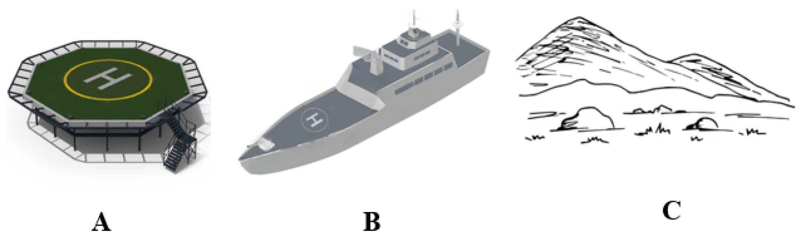
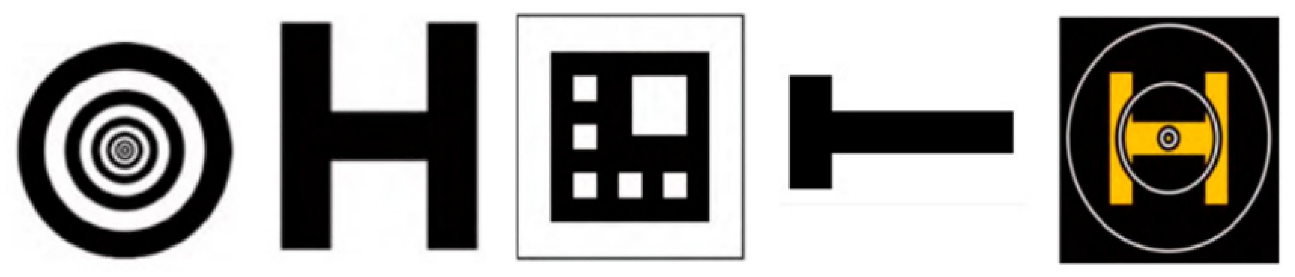
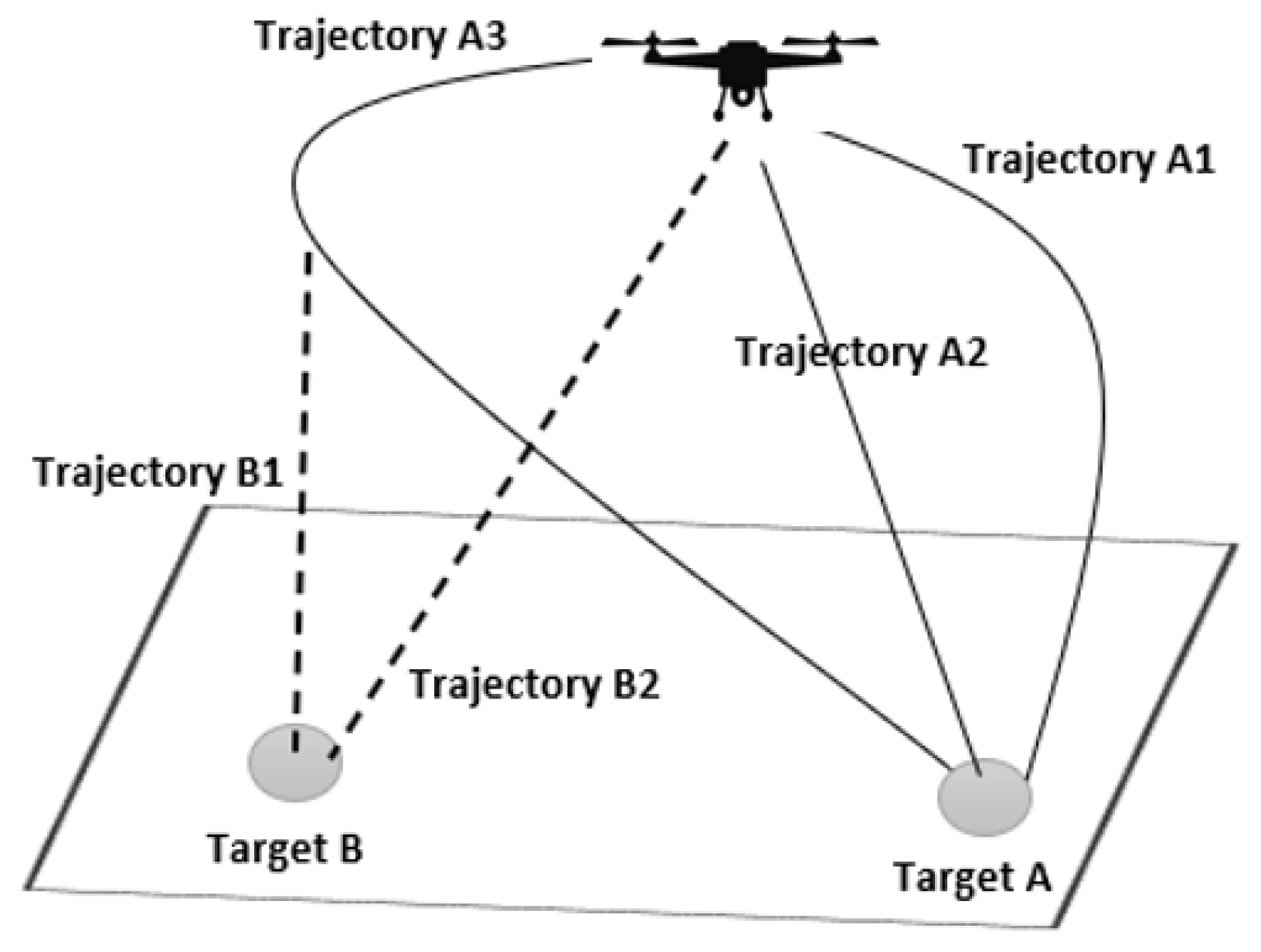
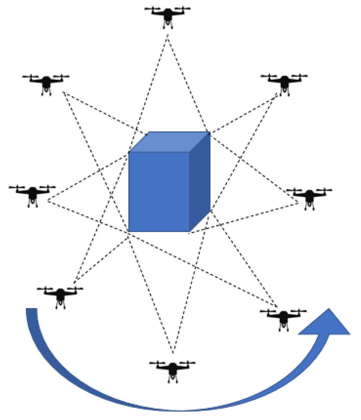
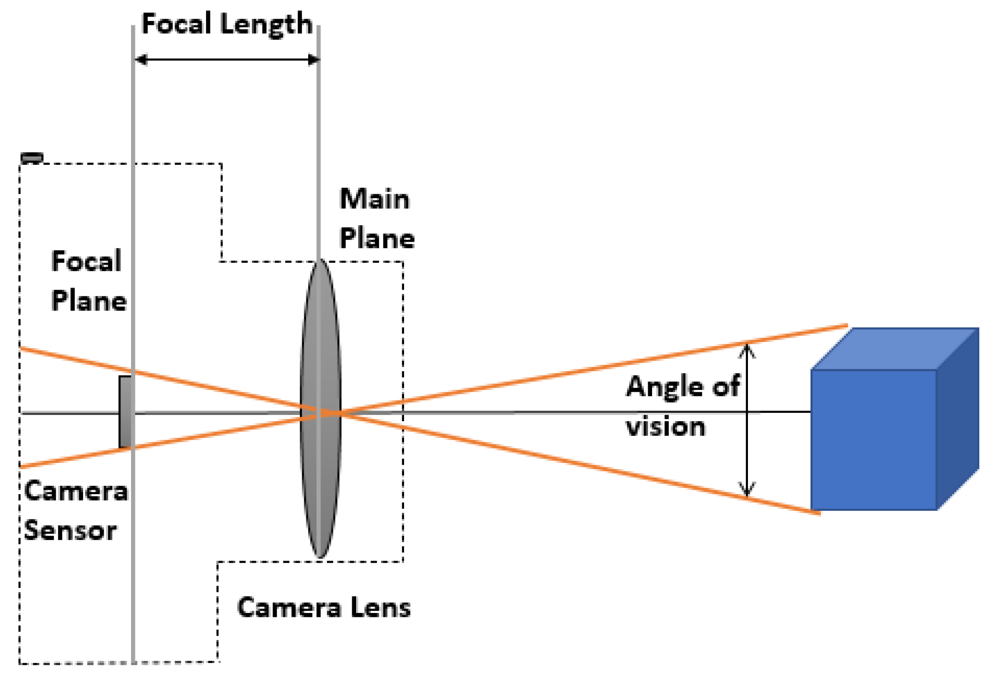
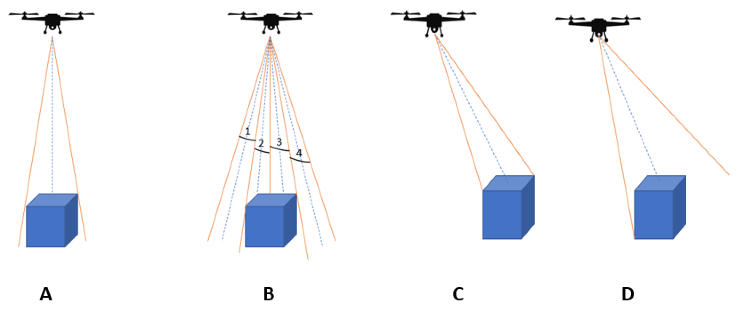
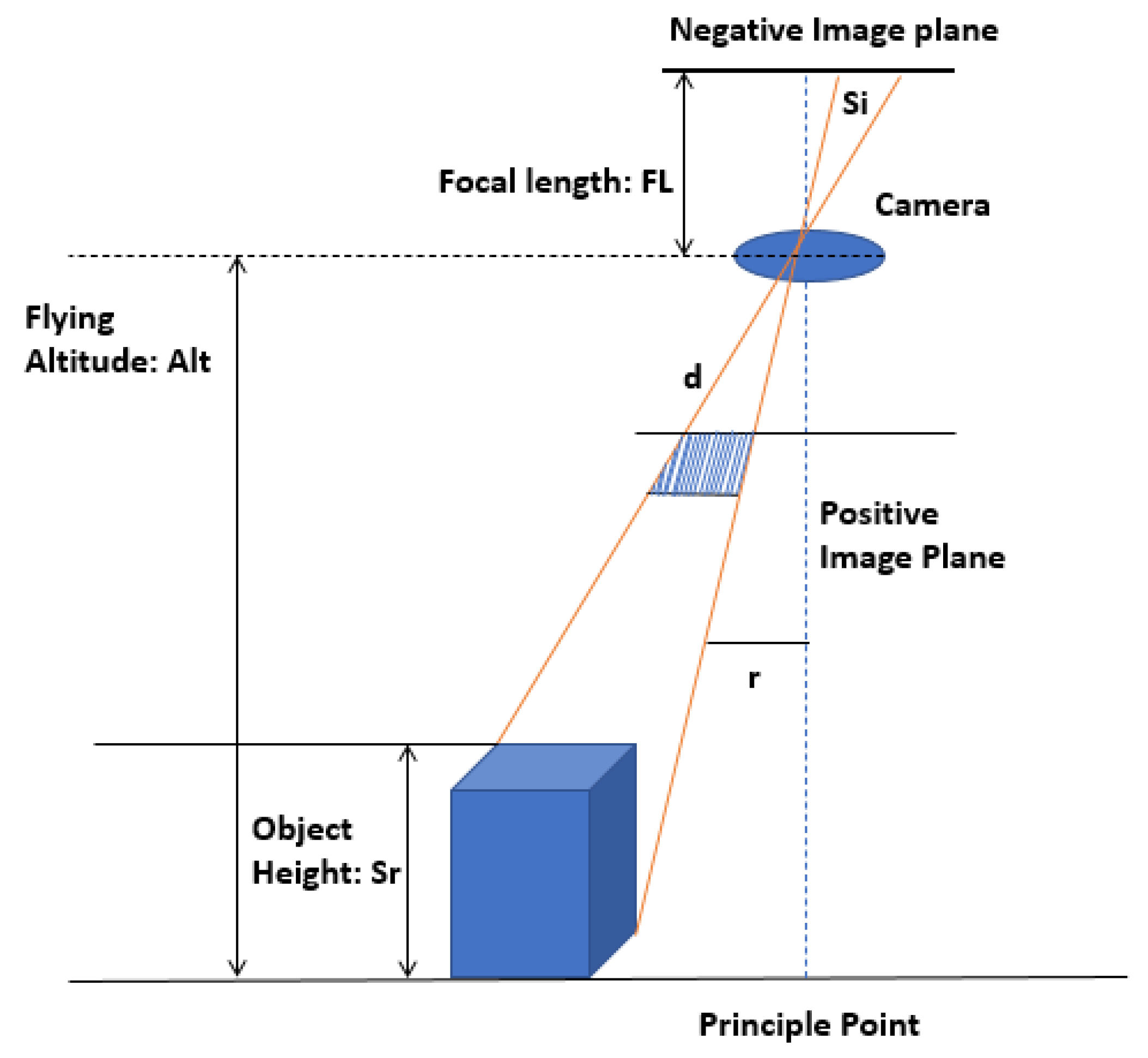
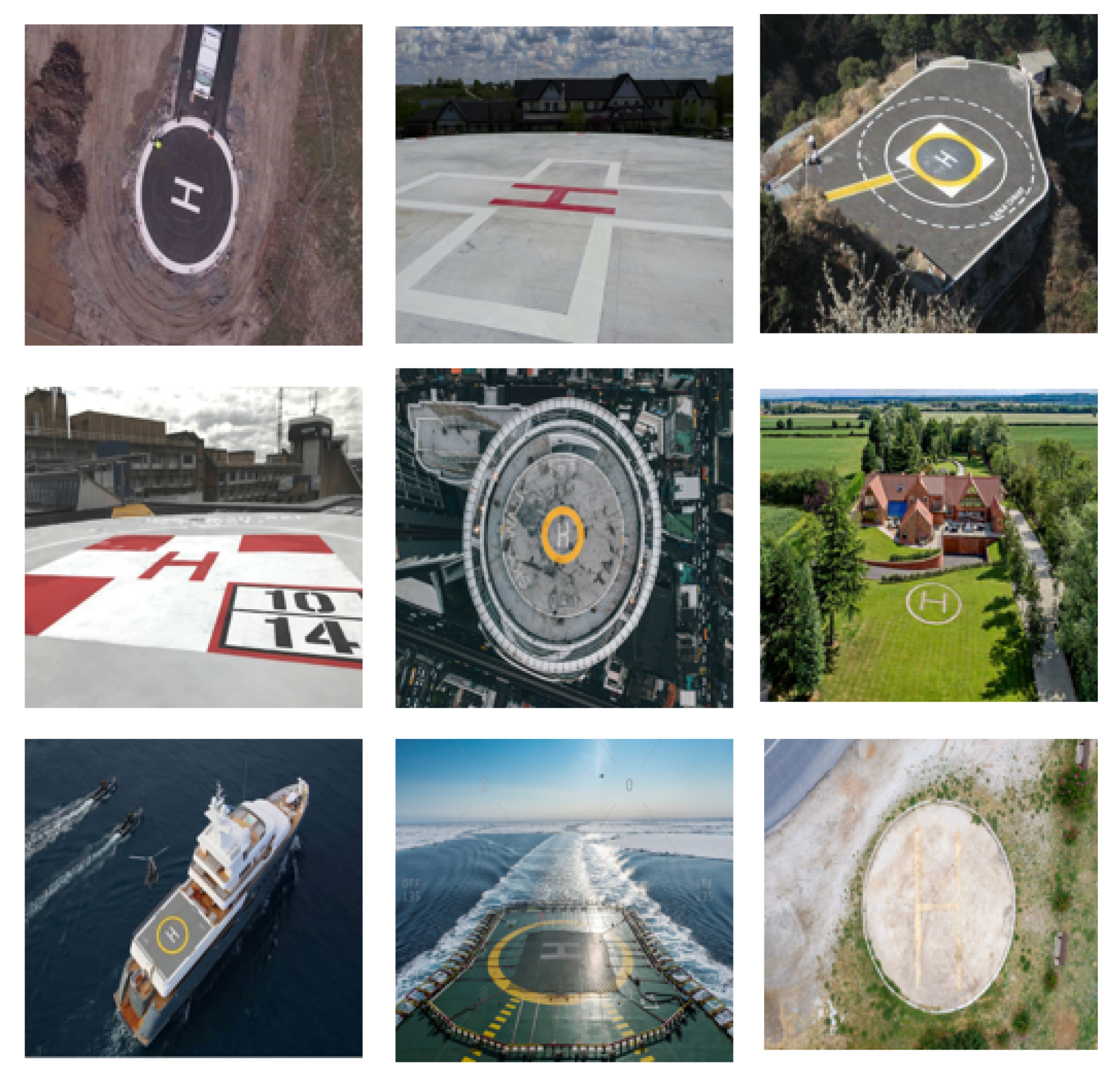
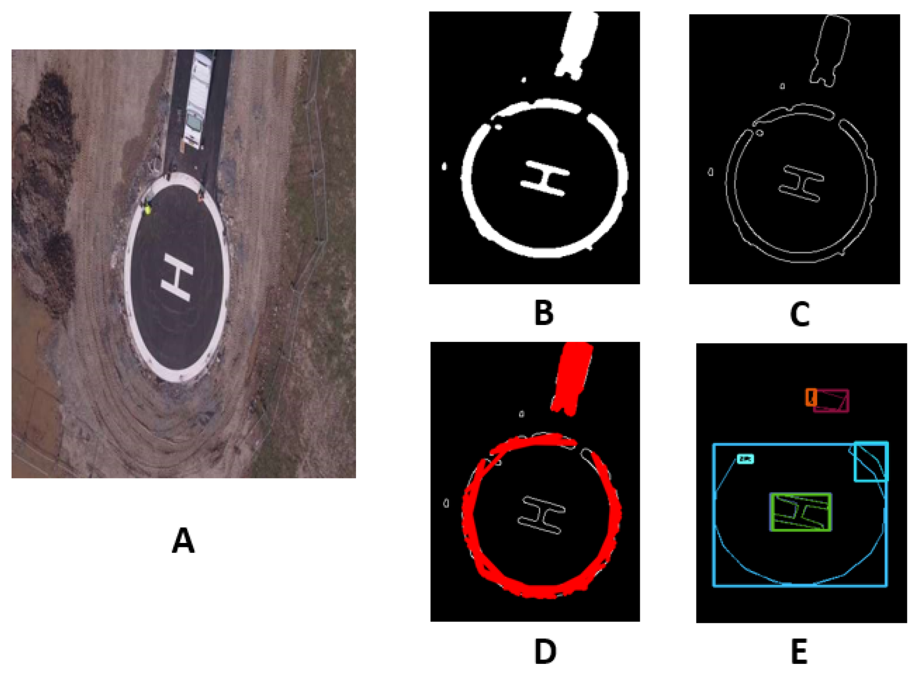
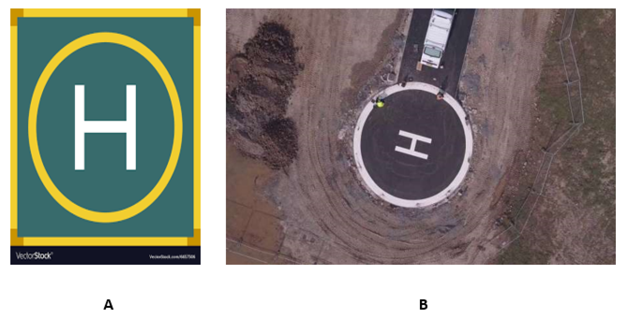
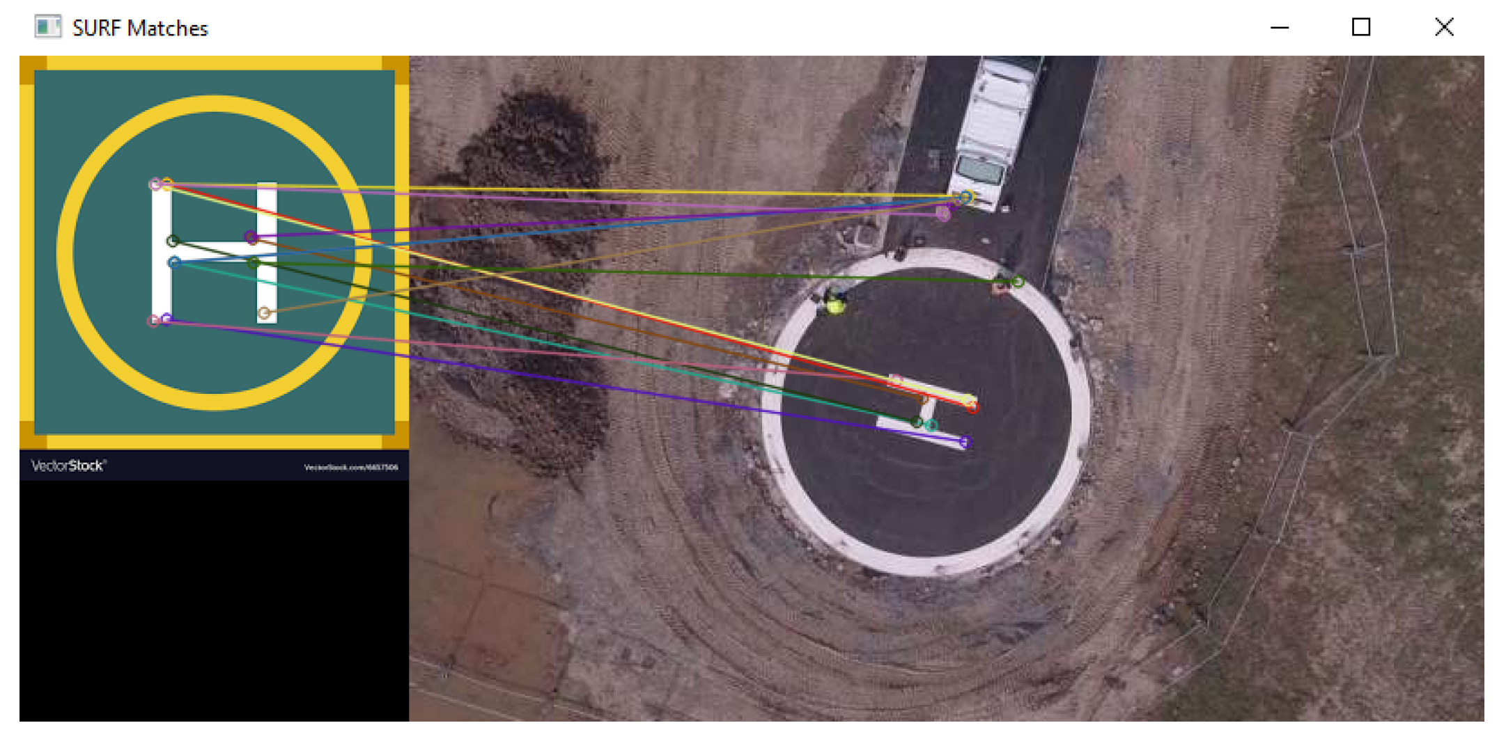
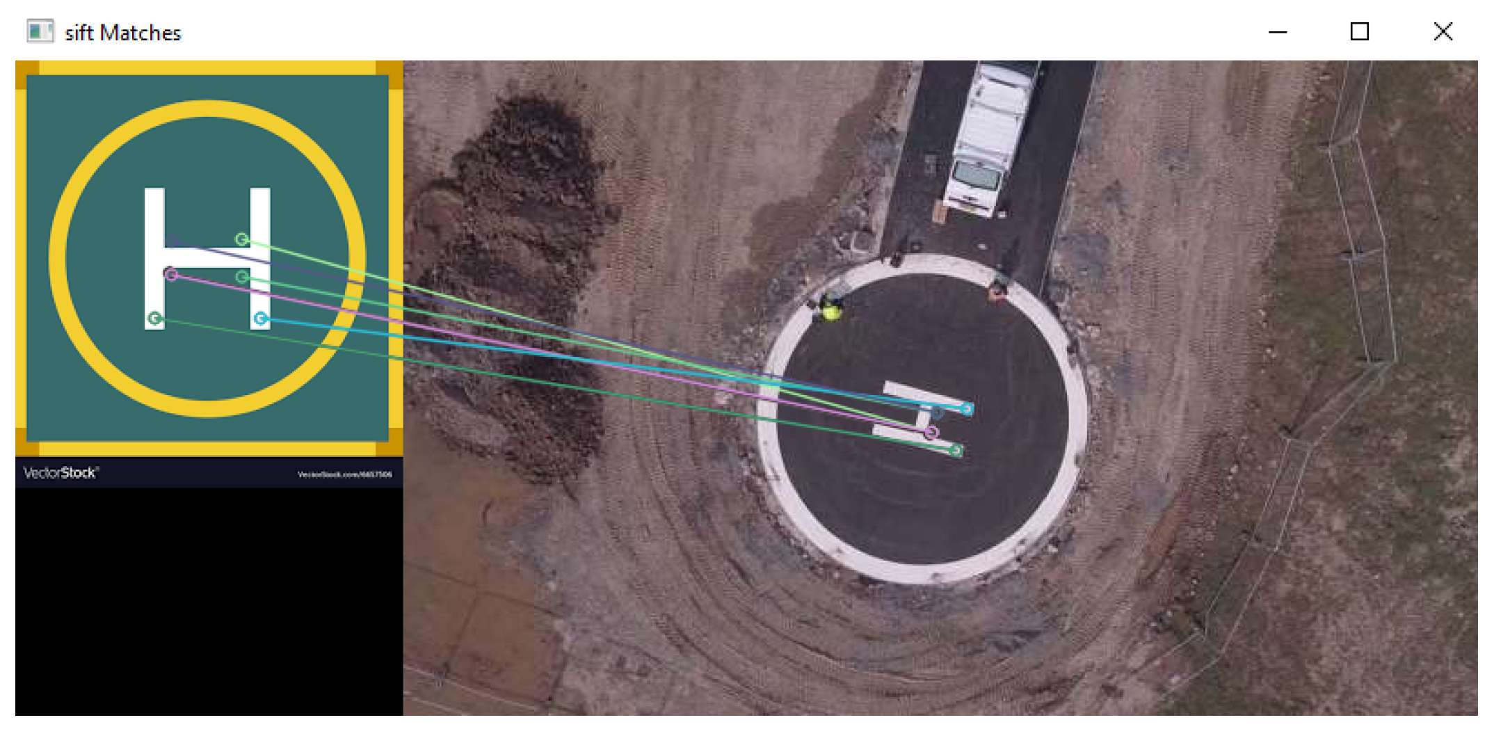
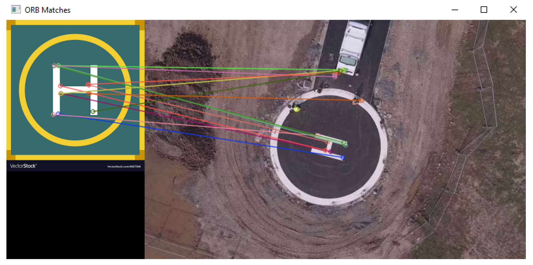
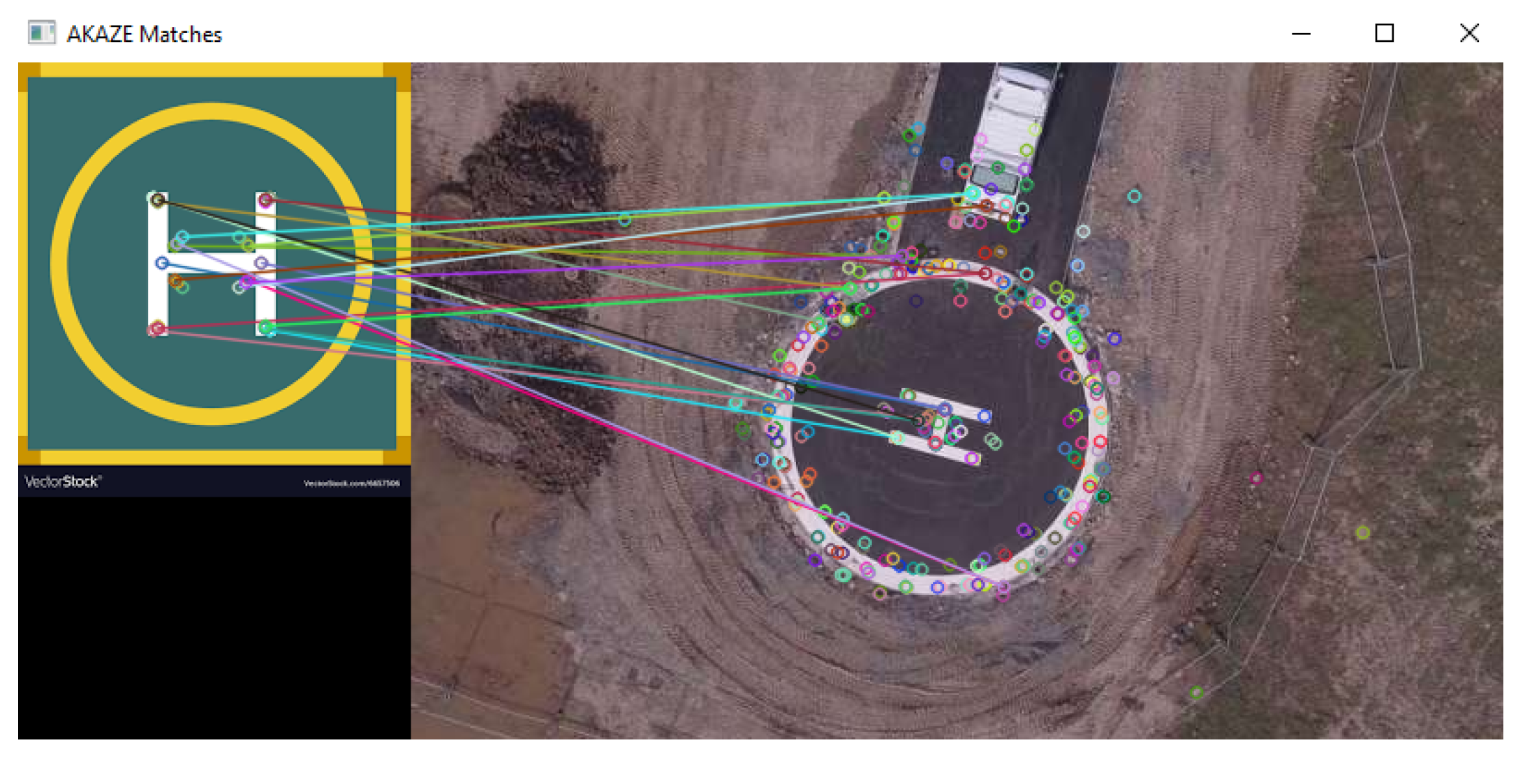
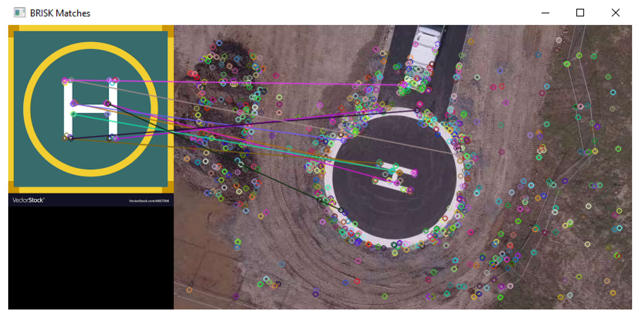
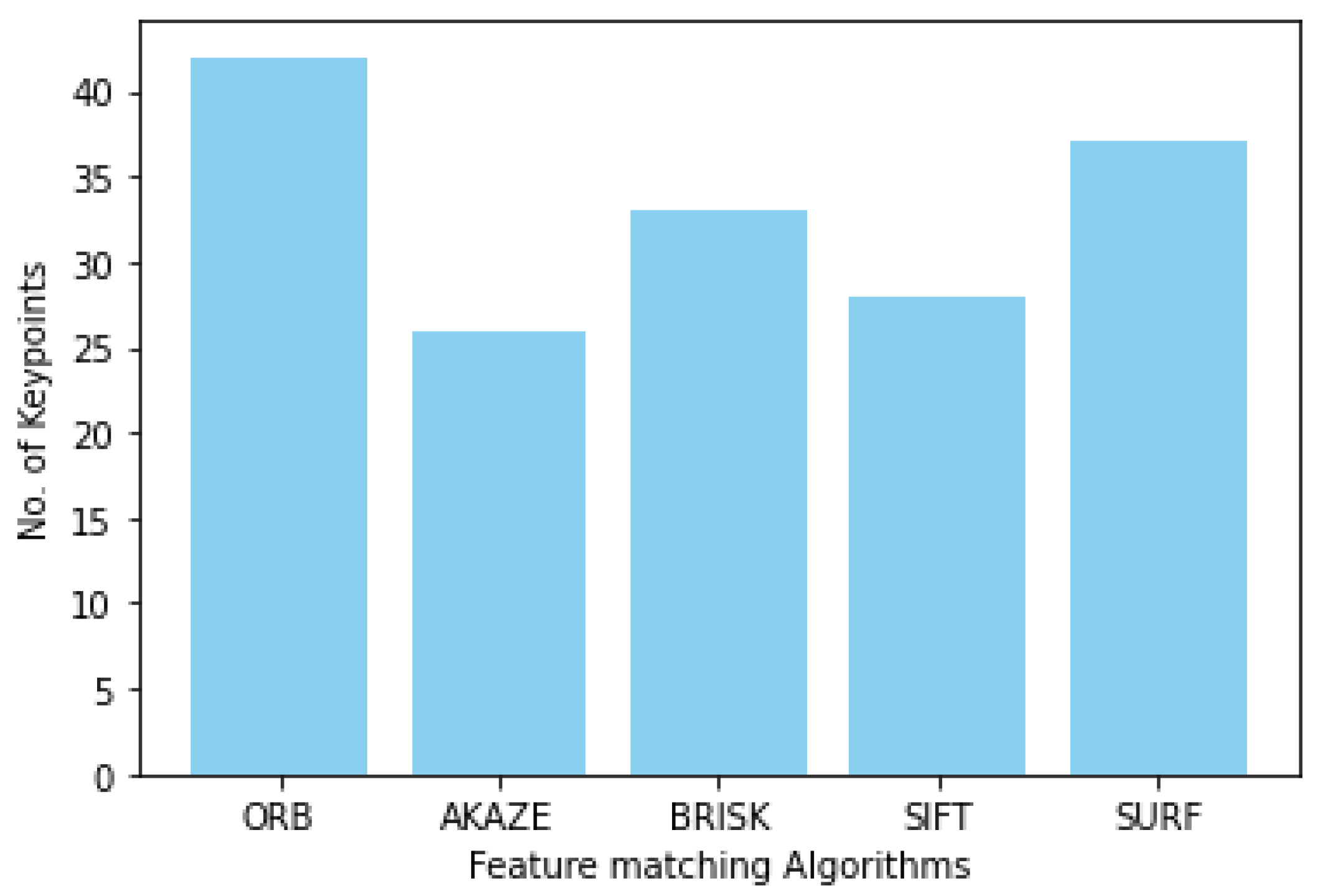
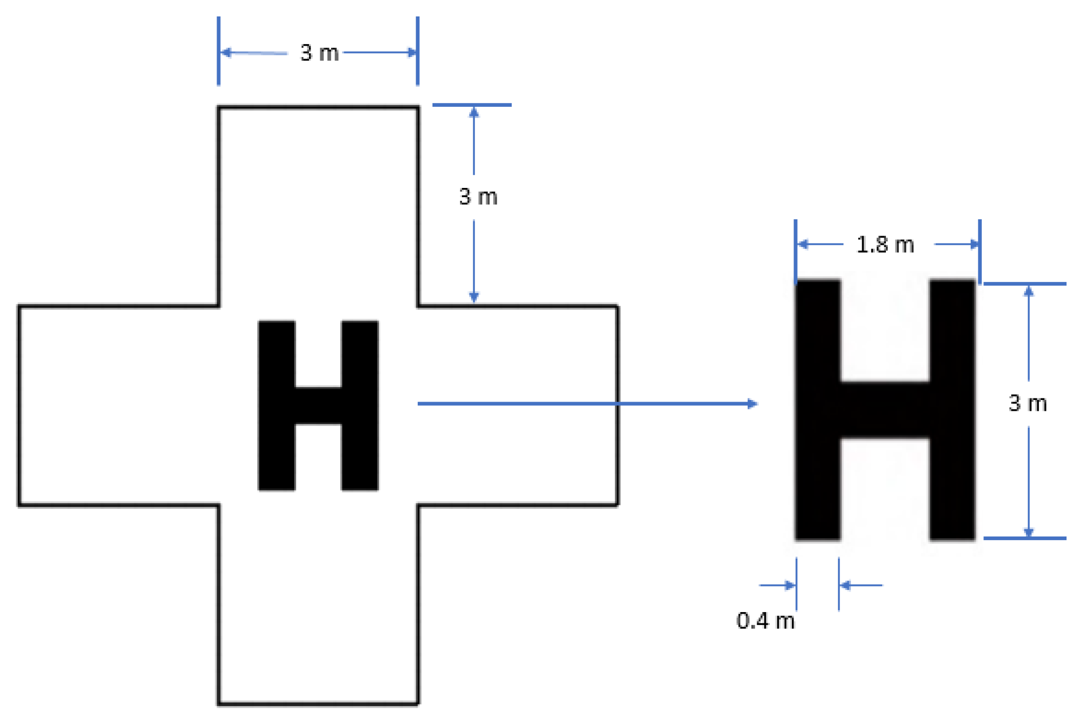