Yield Prediction of Four Bean (Phaseolus vulgaris) Cultivars Using Vegetation Indices Based on Multispectral Images from UAV in an Arid Zone of Peru

Abstract

In Peru, common bean varieties adapt very well to arid zones, and it is essential to strengthen their evaluations accurately during their phenological stage by using remote sensors and UAV. However, this technology has not been widely adopted in the Peruvian agricultural system, causing a lack of information and precision data on this crop. Here, we predicted the yield of four beans cultivars by using multispectral images, vegetation indices (VIs) and multiple linear correlations (with 11 VIs) in 13 different periods of their phenological development. The multispectral images were analyzed with two methods: (1) a mask of only the crop canopy with supervised classification constructed with QGIS software; and (2) the grids corresponding to each plot (n = 48) without classification. The prediction models can be estimated with higher accuracy when bean plants reached maximum canopy cover (vegetative and reproductive stages), obtaining higher R² for the c2000 cultivar (0.942) with the CIG, PCB, DVI, EVI and TVI indices with method 2. Similarly, with five VIs, the camanejo cultivar showed the highest R² for both methods 1 and 2 (0.89 and 0.837) in the reproductive stage. The models better predicted the yield in the phenological stages V3–V4 and R6–R8 for all bean cultivars. This work demonstrated the utility of UAV tools and the use of multispectral images to predict yield before harvest under the Peruvian arid ecosystem.

1. Introduction

Bean (Phaseolus vulgaris) is a legume that constitutes one of the main sources of food; it is a rich and economical source of proteins (20% to 25%) and carbohydrates (50% to 60%) for a large portion of consumers worldwide, mainly in developing countries [1]. It is widely cultivated [2] for its enormous genetic diversity, provides a considerable gene pool for adaptations to future climatic stresses [1] and will probably play a key role in ensuring food security for millions people around the world [3]. According to the Food and Agriculture Organization of the United Nations (FAO), the world population has to find new solutions to increase food production by 70% by 2050. The cultivated area of beans in Peru in 2019 was of 75,390 ha, and it amounted to 0.8% of the gross value of production from agricultural activity [4]. Therefore, improving crops yield represents a great challenge [5], and under climate change conditions, the quantitative evaluation of variables that improve yield is becoming a high priority [6]. Among these traits, biomass, plant height, chlorophyll content and other variables might be an alternative to manage available resources and reduce inputs for production (precision agriculture) [7]. However, crop evaluating techniques must be adapted to different growth stages (phenology) and should involve a low amount of time and resources.

To carry out photosynthesis, plants absorb part of the light emitted by the sun and reflect the rest. This reflected light is analyzed by vegetation indices to detect plants and assess their status. In summary, healthy plants are rich in chlorophyll and reflect more green and near-infrared (NIR) light than those with stressed or dead leaves [8].

To monitor these crops, UAVs were used, which are tools that allow crop monitoring and which facilitate non-contact data collection over a crop area, allowing for the characterization of spatial–temporal information of the field. They are coupled to remote sensors, such as multispectral cameras, thus allowing the estimation of different vegetation indices, providing a faster method to collect field information [9]. Recently, in northern China, researchers conducted an analysis using UAV images that predicted corn crop yields [10]. Similarly, aerial biomass was estimated in various crops, such as sunflower [11], corn [12] and wheat [13]. Mwinuka et al. [14] estimated the Normalized Difference Vegetation Index (NDVI) and Optimized Soil Adjusted Vegetation Index (OSAVI) to predict the yield of eggplant during its vegetative stage. Parker et al. [15] and Santos et al. [16] highlighted the application of UAV for phenotyping (diversity and genetic improvement of crops) and the identification of the variability of crop fields. In this last year, in Peru, some efforts are being conducted to employ UAV + remote sensors to predict the yield for some crops. Recently, the yield of maize was estimated using VIs from multispectral images [17]. Moreover, indices from RGB images were employed to estimate the height of a bean crop [18]. However, it is still necessary to generate more data and methodologies adapted to our conditions since Peru possesses 84 out of the 104 life zones that exist in the world.

Estimating the yield of local commercial bean varieties with multispectral images and sensors with a greater number of bands might be of help to the production system of this crop. The objective of this work was to determine the correlation of different VIs obtained by UAV multispectral images to develop predictive models of performance in four Phaseolus vulgaris cultivars. This technology will make adequate and efficient use of resources and inputs in agricultural production and research applied to crops.

2. Materials and Methods

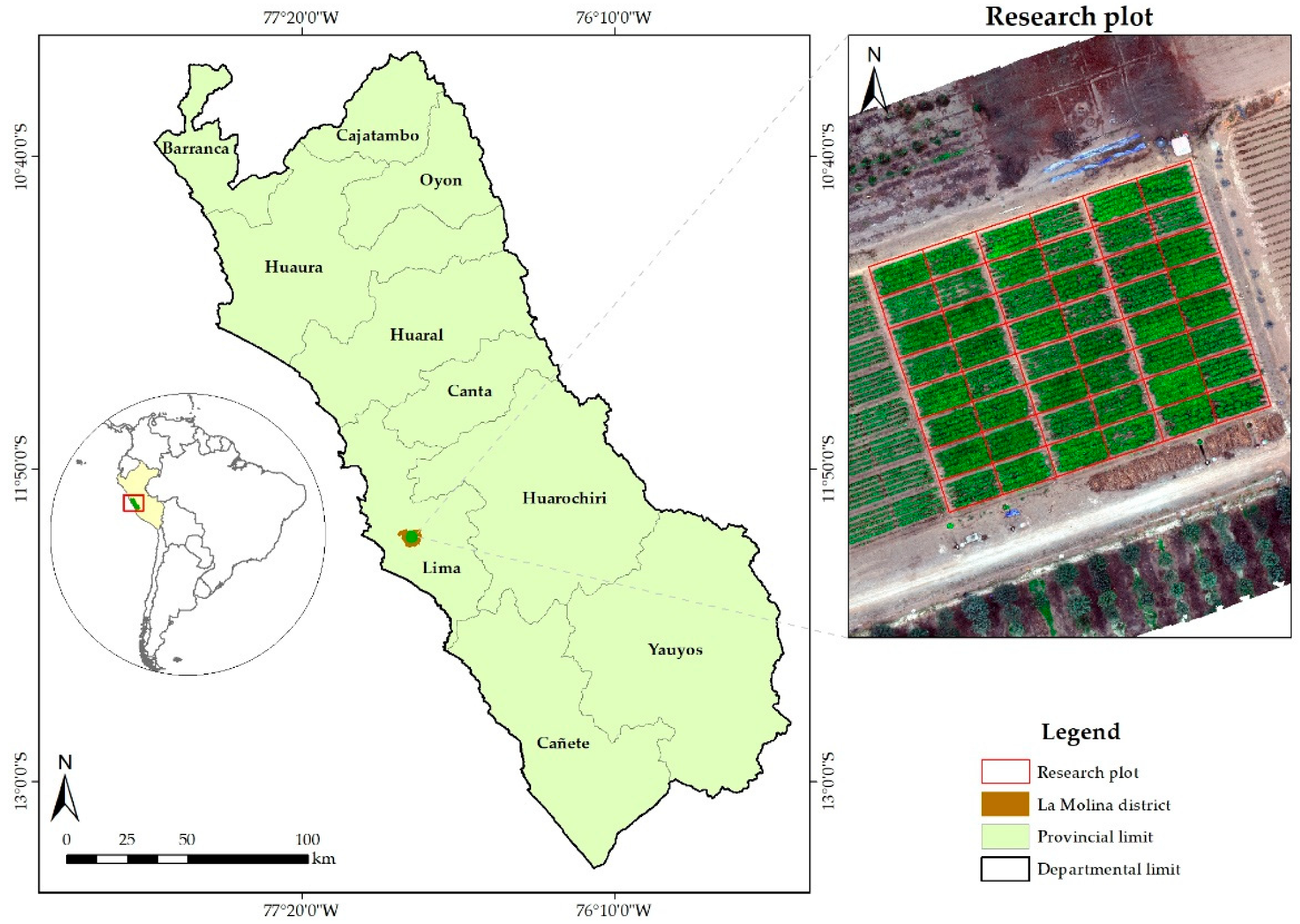
2.1. Study Area

The study area was located at La Molina Research Station of the Instituto Nacional de Innovación Agraria (INIA) (12°4′ S, 76°56′ W, altitude 240 m a.s.l.), La Molina, Lima (Peru). The bean cultivation period was developed during the winter–spring seasons (June–November 2021), using commercial varieties developed by INIA. According to the Warren Thornthwaites climate classification [19], the study area is arid with maximum and minimum temperatures of 33° and 10 °C, respectively, and total annual rainfall of 18 mm in 2021. The meteorological data were recorded in an automatic station (VANTAGE Pro2 Plus Davis, Hayward, CA, USA) (Figure S1), located in the experimental plot. The type of soil is sandy loam with physical characteristics of electrical conductivity (EC) of 0.70 dS/m, pH of 7.41, field capacity of 14.7%, wilting point of 7.6% and bulk density of 1.54 g/cm³ (INIA-Water, Soil and Foliar Research Laboratory). The experimental design was split-plots with a randomized complete block design, including four irrigation treatments and three replicates and subplots of four commercial bean varieties (canario 2000 (C2000), camanejo, cifac, costacen) (Figure 1). Each experimental plot was 36 m² with five rows (8 m long and 4.5 m wide). Four irrigation treatments were applied according to the reference evapotranspiration (ETo), using the FAO Penman–Monteith methodology, which included a control irrigation (100% ETo) and another three with 120% ETo, 80% ETo and 60 ETo %. They were applied from flowering to maturity, and previous irrigations were similar to control. The drip irrigation system had a discharge rate of 3.75 l/h with a spacing between drippers of 0.25 m.

2.2. Plant Height Measurement

Plant height was measured manually from the soil surface to the highest stem apex in the plant on a metric scale (cm) with an equal number of samples (n = 48) at each monitoring date (26, 33, 40, 47, 54, 61, 68, 77, 82 and 89 days after sowing, DAS).

2.3. Measurement of Chlorophyll Content

Chlorophyll content estimation was performed using a SPAD meter (SPAD-502 Minolta Co, Osaka, Japan) at 26, 33, 40, 47, 54, 54, 61, 68, 82 and 89 DAS. SPAD values were measured on a representative plant free of mechanical damage by choosing fully developed leaves from the upper third just after the flight mission on the day and time of each UAV inspection. Three readings were taken per experimental unit, with a total of forty-eight samples for each evaluation date.

2.4. Measurement of Dry Aerial Biomass and Yield

The aerial biomass was determined at 26, 40, 54, 68 and 82 DAS in the bean crop—with a number of samples n = 48—of stems, leaves and pods, which were placed in a stove (VENTICELL model LSIS-B2V/CV 404, Munich, Germany) at 103 °C for 24 h and weighed to calculate the dry biomass. The sampling was carried out in an area of 0.13 m² of each experimental unit. The yield of the grain crop at 12–14% of commercial moisture was evaluated considering the plot of 36 m²; these values were projected to tons per hectare (t/ha).

2.5. Estimation of Vegetation Indices

To acquire multispectral images, we employed a quadcopter-type platform, DJI Matrice 300 RTK (Shenzhen Dajiang Baiwang Technology Co., Ltd., Shenzhen, China). A dual multispectral camera MicaSense RedEdge-Mx + RedEdge-MX Blue (MicaSense, RedEdge, NC, USA) with ten multispectral bands (Coastal blue 444, Blue 475, Green 531, Green 560, Red 650, Red 668, Red Edge 705, Red Edge 717, Red Edge 740 and NIR 842) with a 1.2 MP global shutter was coupled to this UAV. The images were collected on 13 dates (33, 40, 47, 54, 61, 68, 76, 82, 89, 97, 103, 110 and 118 DAS) (Figures S1 and S2)—sunny days with wind speeds less than 12 m/s—between 11:00 a.m. to 01:00 pm [20]. The flight plan was made with the DJI Pilot 2 UAV application, considering a frontal and lateral overlap of 80%, height of 30 m, speed of 4.5 m/s and the camera focused on the nadir (perpendicular to the ground surface), allowing a resolution of 2.08 cm/pixel to be obtained for multispectral images for each pixel. The processing was performed with the Pix4Dmapper Pro software (V4.8.0, Pix4D S.A., Prilly, Switzerland) and it was used for the construction of orthomosaics, reflectances and Digital Surface Models (DSM).

In addition, the geometric correction was performed with nine control points previously installed and registered with differential Global Navigation Satellite System (GNSS) (South Galaxy G1 model, South Surveying and Mapping Instrument Co., Ltd., Guangdong, China). For the radiometric calibration of the multispectral images, the reflectance calibrator panel and a DLS 2 light sensor with built-in GPS (Automatic Calibration Panel Detection for MicaSense) that adjusts the readings to ambient light were used [11]. Then, the image mosaic processing was specifically designed to process UAV images using techniques based on both machine vision and photogrammetry.

The entire processing workflow was as follows: (i) initialize all geolocated images captured on each flight by automatically finding feature tie points in matching image pairs and correcting them based on camera model; (ii) nine ground control points were incorporated to correct the geographic coordinates of the images; (iii) densified point clouds were then generated with a 7 × 7 pixel matching window; (iv) finally, the digital surface model and the orthophoto with a spatial resolution of 2.08 cm were generated using the inverse distance weighting method. Vegetation indices were widely applied to predict crop yield [17,21], according to

Table 1. Vegetation indices applied for bean cultivars on different evaluated dates.

Indices	Equation	Source
Normalized Difference Vegetation Index (NDVI)	$\frac{NIR-RED}{NIR+RED}$	[22]
Green Normalized Difference Vegetation Index (GNDVI)	$\frac{NIR-GREEN}{NIR+GREEN}$	[23]
Normalized Difference RedEdge Index (NDRE)	$\frac{NIR-REDEDGE}{NIR+REDEDGE}$	[24]
ChlorophyII Index Green (CIG)	$\left(\frac{NIR}{G}\right)-1$	[24]
Plant Cell Density (PCB)	$\left(\frac{NIR}{R}\right)$	[25]
Soil Adjusted Vegetation Index (SAVI)	$\frac{\left(NIR-RED\right)\left(1+L\right)}{NIR+RED+L}$	[26]
ChlorophyII Vegetation Index (CVI)	$\frac{NIR\times RED}{GREE{N}^2}$	[27]
ChlorophyII Index-RedEdge (CIRE)	$\frac{NIR}{REDEDGE}-1$	[28]
Difference Vegetation Index (DVI)	$NIR-REDEDGE$	[28]
Enhanced Vegetation Index (EVI)	2.5 × ((NIR − RED)/((NIR) + (6 × RED) − (7.5 × BLUE) + 1))	[28]
Triangular Vegetation Index (TVI)	0.5 × (120 × (NIR − GREEN) − 200 × (RED − GREEN)	[28]

.

In this study, we used two methods for the analysis of multispectral images: (i) a mask was built only for the crop canopy with supervised classification constructed with QGIS software [29] (method 1) (Figure S2); and (ii) the grids corresponding to the average of each plot (n = 48) without classification were made to obtain the values and indices of reflectance including the ground (method 2) (Figure S3).

2.6. Data Analysis and Model Development

We employed a split-plot design and data were analyzed with an analysis of variance (ANOVA) and mean difference, with the Duncan test with an alpha = 0.05. Correlation analyses were also performed with the Pearson-r estimator of yield and vegetation indices. The data collected in this work were recorded in a field book according to the field plots (n = 48) and were analyzed with software R v.4.2.2 [30] and RStudio v.7.2.576 [31] software with packages, namely, GGally [32], ggplot2 [33] and agricolae [34] to carry out descriptive statistics and determine the relationships between the variables of the images. Field reference measurements were tested to determine a significant correlation with two statistical indicators—the Pearson correlation coefficient (r) and p-value—for significance. The evaluated dates were grouped by varieties and their phenological stages: vegetative (33–47 DAS), reproductive (54–68 DAS), ripening (76–97 DAS) and senescence (103–118 DAS), considering the average values of the 11 VIs obtained by the two classification methods of the multispectral images, with a Pearson-r > 0.45. For the development of performance prediction models, multiple linear regression was used. Model estimation was obtained from method 1 and 2 by combining three to five VIs for each bean cultivar and phenological stages. For the multivariate analysis, a principal component analysis (PCA) was used using R software packages, factoextra [35] and FactoMiner [36], to discriminate the dates of evaluation for the VIs evaluated from multispectral images obtained from UAV for different stages of vegetative development of the four commercial beans.

3. Results

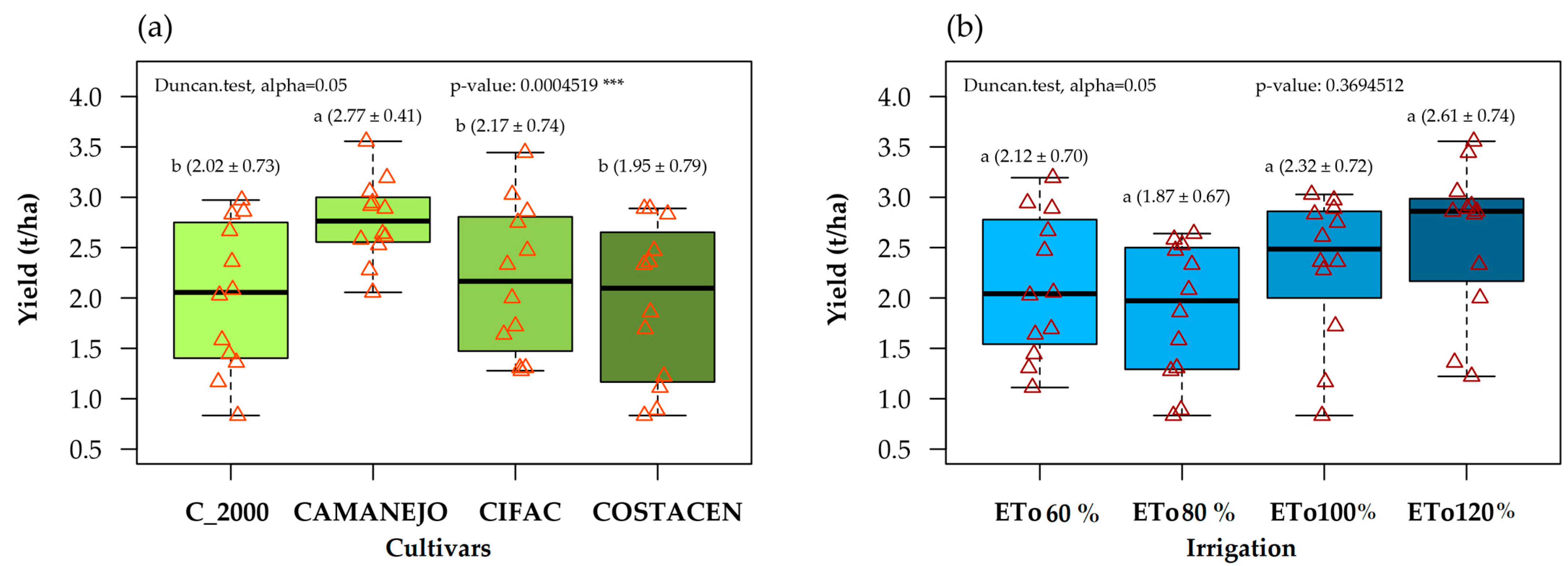
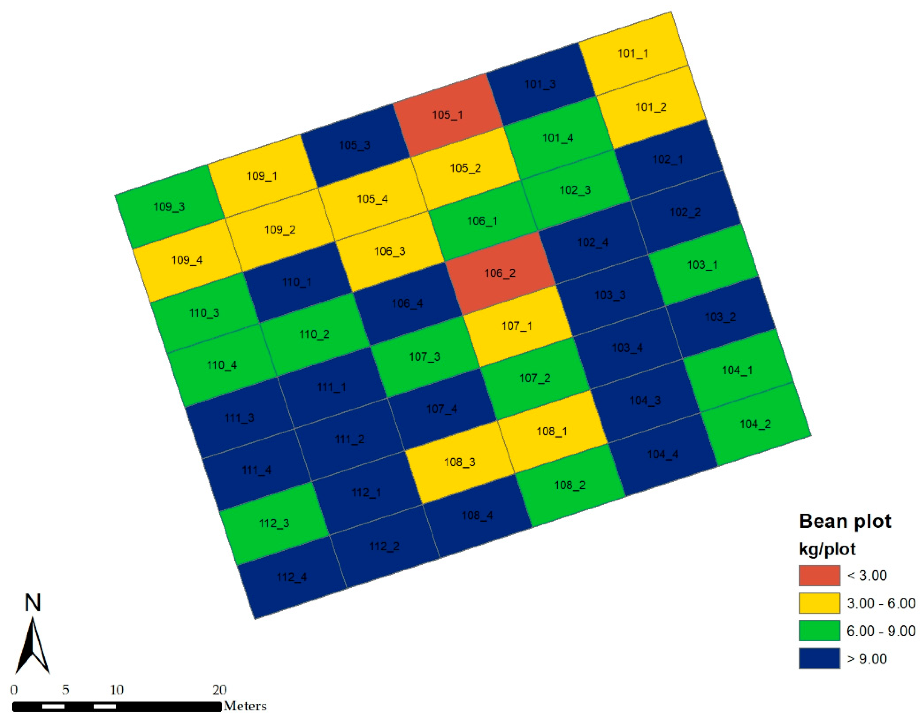
3.1. Effects of Irrigation Treatments and Grain Yield of Bean Varieties

In the ANOVA analysis, we only found differences for bean varieties. The camanejo cultivar obtained the highest yield (2.77 ± 0.41 t/ha) in dry grain (approx. 12% humidity) and the other varieties had similar yields (mean Sq: 1.19142, F value: 8.6594) (Figure 2a). There were no yield differences under the irrigation treatments at 120, 100, 80 and 60% Eto referential (mean Sq: 1.68836, F value: 1.2585) (Figure 2b). Moreover, we did not find significant interaction between cultivars × irrigation (mean Sq: 0.13852, F value: 0.7105).

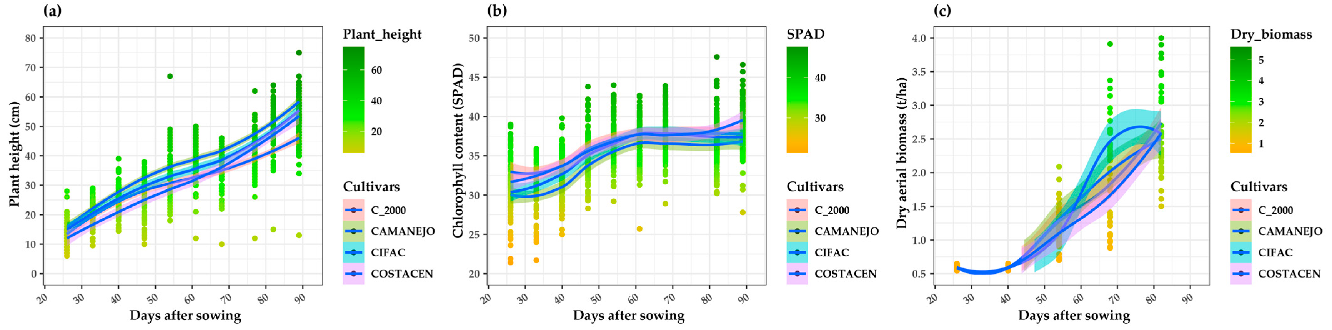
3.2. Variables Evaluated during the Development of the Bean Crop

We observed a continuous increment for means of the plant height variable (13.28 ± 3.65, 20.99 ± 3.78, 25.81 ± 5.13, 25.79 ± 6.09, 33.78 ± 7.17, 36.84 ± 6.17, 34.95 ± 6.49, 43.22 ± 7.16, 49.46 ± 7.34 and 52.37 ± 8.52 cm, respectively) for each evaluation date between 26 at 89 DAS (Figure 3a), coinciding with its phenological development, with a growth rate of 4.34 ± 3.63 cm approximately for each week, a 17% increase in three cultivars (c2000, cifac and camanejo) and 20% in costasen. The dry biomass variable exhibited a similar trend (0.59 ± 0.03, 0.59 ± 0.03, 1.19 ± 0.29, 1.99 ± 0.72 and 3.04 ± 1.08 t/ha, respectively) at 26, 40, 54, 68, y 82 DAS (Figure 3c). The greatest increase in dry biomass evaluated at 54 DAS was for camanejo, with 120% compared to the previous sampling. Cifac showed an increase at 61 DAS up to 125% in aerial dry biomass On the other hand, the SPAD chlorophyll content variable stopped its increase at 54 DAS (Figure 3b) (31.64 ± 3.83, 30.89 ± 3.11, 32.19 ± 3.03, 35.12 ± 3.45, 37.19 ± 3.10, 36.59 ± 2.75, 38.09 ± 2.92, 36.15 ± 3.47, 38.54 ± 3.29 and 37.51 ± 3.05 SPAD, respectively), coinciding with the phenological stage of flowering (R5) and maximum foliage coverage in the plants; this continued until the R8 phase.

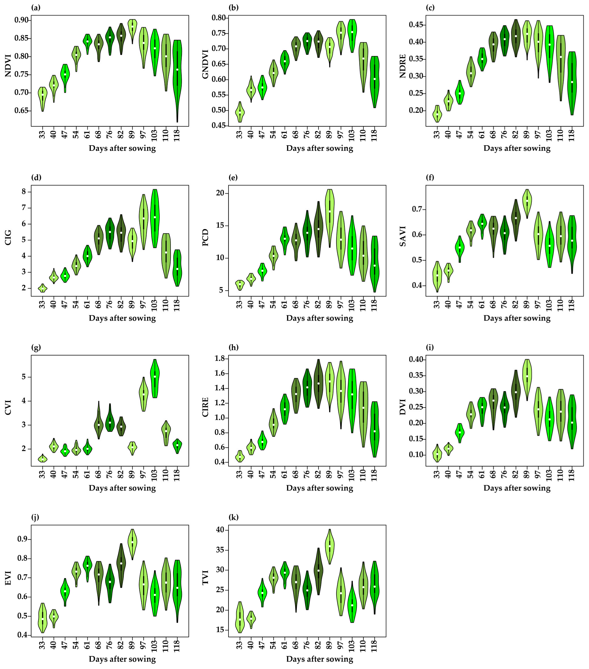
3.3. Vegetation Indices Estimated

The VIs was calculated from the multispectral images on each evaluation date (13 dates in total) (Table S1). They showed a continuous increase as the height of the plant developed in the early stages of development (Figure 3a). The first seven indices had a similar trend with respect to the different evaluation dates for plant height during the vegetative development of the crop (Figure 4); the highest mean values of these indices were determined between 76 to 97 DAS with NDVI (0.88) (Figure S4) GNDVI (0.75), NDRE (0.42) (Figure S5), CIG (6.27), PCB (17.11), SAVI (0.73) and CIRE (1.48) (Figure 4a–g). CVI, DVI, EVI and TVI indices did not show this trend; on the contrary, their highest mean values were observed at 103 DAS for CVI (4.92) and 89 DAS for EVI (0.35) and TVI (0.88) (Figure 4h–k and Table S1).

On the other hand, when performing the analyses of the multispectral images with method 2 (Table S2), the maximum vegetation indices estimated decreased between 35–25% with respect to method 1, PCB (−35%), TVI (−34%), DVI (33%), EVI (31%), SAVI (29%), CIRE (27%), NDVI (25%) and CIG (25%), respectively. In the case of CVI, it increased 1% compared to method 1. The GNDVI and NDRE indices also decreased 12 and 23%, respectively, using method 2.

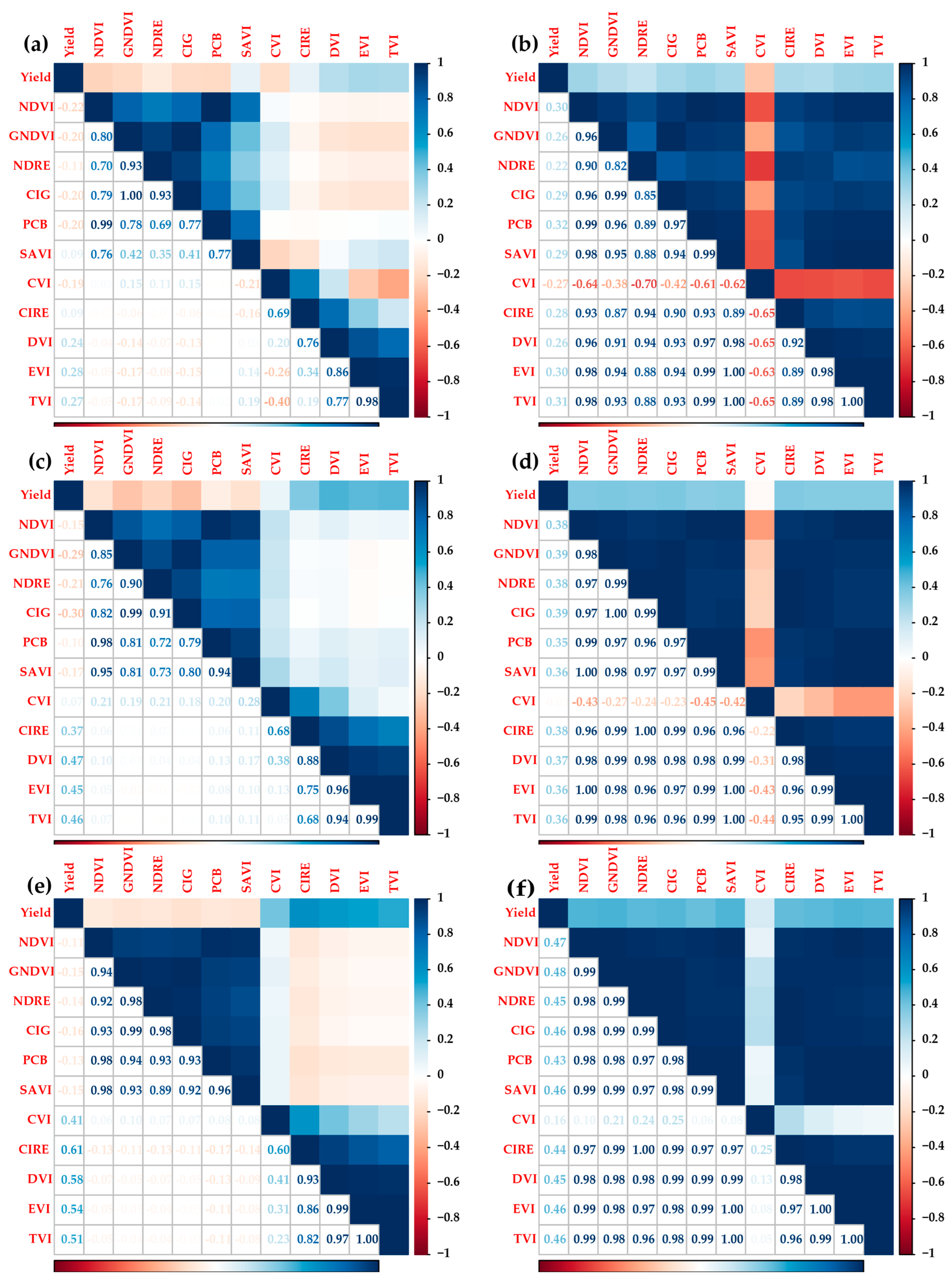
3.4. Pearson-r Correlation of Vegetation Indices and Yield

With method 1, the highest significant correlations between VIs and yield were observed after 61 DAS (

Table 2. Pearson-r correlations of bean yield with 11 VIs (NDVI, GNDVI, NDRE, CIG, PCB, SAVI, CVI, CIRE, DVI, EVI and TVI) evaluated on 13 dates during their vegetative development with supervised classification to generate the mask only from the crop canopy (method 1).

DAS	NDVI		GNDVI		NDRE		CIG		PCB		SAVI		CVI		CIRE		DVI		EVI		TVI
33	−0.259		−0.158		−0.127		−0.159		−0.298	*	0.314	*	−0.321	*	−0.23		0.001		0.138		0.130
40	−0.218		−0.246		−0.103		−0.252		−0.210		−0.139		−0.184		0.184		0.291	*	0.288	*	0.281
47	−0.092		−0.131		−0.076		−0.111		−0.063		−0.047		−0.069		0.214		0.319	*	0.313	*	0.317	*
54	−0.072		−0.123		−0.080		−0.111		−0.038		−0.050		−0.002		0.313	*	0.360	*	0.298	*	0.354	*
61	−0.120		−0.179		−0.211		−0.164		−0.080		−0.137		0.208		0.375	**	0.475	***	0.420	**	0.411	**
68	−0.135		−0.327	*	−0.250		−0.331	*	−0.079		−0.168		0.035		0.399	**	0.496	***	0.500	***	0.489	***
76	−0.008		0.013		0.016		0.008		−0.039		−0.024		0.184		0.534	***	0.514	***	0.453	***	0.429	***
82	−0.092		−0.165		−0.145		−0.163		−0.094		−0.148		0.447	***	0.566	***	0.555	***	0.515	***	0.497	***
89	−0.055		−0.124		−0.137		−0.145		−0.092		−0.074		0.409	**	0.568	***	0.543	***	0.507	***	0.453	***
97	−0.109		−0.116		−0.097		−0.131		−0.103		−0.125		0.417	**	0.628	***	0.620	***	0.599	***	0.576	***
103	−0.177		−0.162		−0.128		−0.159		−0.167		−0.172		0.507	***	0.633	***	0.636	***	0.611	***	0.587	***
110	−0.081		−0.054		−0.018		−0.047		−0.049		−0.130		0.508	***	0.605	***	0.628	***	0.613	***	0.581	***
118	−0.452	**	−0.389	**	−0.377	**	−0.394	**	−0.453	**	−0.460	**	0.046		0.515	***	0.559	***	0.575	***	0.591	***

ns. p-value > 0.05, * p-value < 0.05, ** p-value < 0.01 and *** p-value < 0.001.

), obtaining the maximum directly proportional correlation for the CIRE and DVI indices at 103 DAS (r = 0.633 *** and r = 0.636 ***, respectively). Inversely proportional correlations were also obtained at 118 DAS for six indices (NDVI, GNDVI, NDRE, CIG, PCB and SAVI) and they were highly significant (p-value > 0.001).

Table 3. Pearson-r correlations of bean yield with 11 VIs (NDVI, GNDVI, NDRE, CIG, PCB, SAVI, CVI, CIRE, DVI, EVI and TVI) evaluated on 13 dates during their vegetative development without classification to generate the mask with soil and crop canopy (method 2).

DAS	NDVI		GNDVI		NDRE		CIG		PCB		SAVI		CVI		CIRE		DVI		EVI		TVI
33	0.099		−0.077		−0.120		−0.019		0.203		0.110		−0.288	*	−0.079		−0.003		0.155		0.176
40	0.345	*	0.316	*	0.221		0.325	*	0.331	*	0.313	*	−0.112		0.246		0.260		0.318	*	0.334	*
47	0.363	*	0.374	**	0.355	*	0.359	*	0.342	*	0.332	*	−0.177		0.350	*	0.321	*	0.335	*	0.341	*
54	0.356	*	0.345	*	0.349	*	0.345	*	0.345	*	0.337	*	−0.222		0.347	*	0.332	*	0.332	*	0.341	*
61	0.379	**	0.386	**	0.376	**	0.380	**	0.356	*	0.356	*	−0.105		0.376	**	0.369	**	0.357	*	0.356	*
68	0.384	**	0.410	**	0.387	**	0.400	**	0.351	*	0.381	**	0.086		0.386	**	0.380	**	0.382	**	0.377	**
76	0.395	**	0.418	**	0.389	**	0.405	**	0.359	*	0.384	**	0.195		0.384	**	0.378	**	0.382	**	0.378	**
82	0.426	**	0.443	**	0.419	**	0.424	**	0.382	**	0.419	**	0.246		0.408	**	0.410	**	0.418	**	0.413	**
89	0.484	***	0.471	***	0.449	**	0.441	**	0.427	**	0.471	***	−0.178		0.430	**	0.452	**	0.475	***	0.468	***
97	0.540	***	0.526	***	0.487	***	0.494	***	0.494	***	0.536	***	0.175		0.464	***	0.504	***	0.533	***	0.529	***
103	0.523	***	0.522	***	0.480	***	0.503	***	0.493	***	0.512	***	0.285	*	0.466	***	0.483	***	0.508	***	0.501	***
110	0.533	***	0.507	***	0.474	***	0.482	***	0.491	***	0.540	***	0.108		0.457	**	0.505	***	0.544	***	0.543	***
118	0.525	***	0.470	***	0.439	**	0.453	**	0.470	***	0.533	***	−0.268		0.433	**	0.484	***	0.530	***	0.539	***

ns. p-value > 0.05, * p-value < 0.05, ** p-value < 0.01 and *** p-value < 0.001.

shows correlation of VIs and yield with method 2. Highly significant (***) correlations between 97 to 118 DAS were observed for the following six VIs: NDVI, GNDVI, SAVI, DVI, EVI and TVI (0.543 > r > 0.47).

Yield prediction models with average index values by variety and phenological stage (Figure 5) allowed us to define and establish those models with the highest performance based on the number of indexes combined for the equation. The highest correlation during the vegetative stage was obtained for two commercial bean cultivars—c2000 and camanejo—for both methods (Figure 6a–d).

The Equations (1) and (2) for c2000 are as follows, for method 1 and for method 2, respectively:

Y = 127.7 − 284.90 × NDVI + 73.18 × GNDVI + 6.45 × PCB − 6.85 × CVI + 13.93 × CIRE

(1)

Y = 26.94 − 109.20 × NDVI + 17.55 × PCB − 31.25 × CIRE − 475.58 × EVI + 9.71 × TVI.

(2)

Cultivar camanejo exhibited the following equation for method 1 and method 2 (Equations (3) and (4), respectively):

Y = −49.28 + 109.65 × NDVI − 110.31 × NDRE + 4.51 × CIG − 49.59 × SAVI + 20.31 × EVI

(3)

Y = 65.58 − 61.22 × NDVI + 47.03 × CIG − 7.97 × PC1 − 28.58 × CVI − 43.69 × CIRE.

(4)

On the other hand, the model with the lowest performance in the vegetative stage (Figure 6c,f) was for the cultivar cifac for method 1 and for method 2 (Equations (5) and (6), respectively).

Y = −45.76 − 189.45 × DVI + 293.7 × EVI − 4.25 × TVI

(5)

Y = 1.97 − 480.94 × SAVI + 49.61 × CIRE + 395.43 × EVI

(6)

For the prediction models in the reproductive stage of the four bean cultivars (Figure 7), cifac and costacen obtained the highest correlation for method 1 (Equations (7) and (8), respectively) (Figure 7a).

Y = −22.76 + 17.41 × NDVI + 53.80 × NDRE − 6.08 × CIG + 2.75 × CVI + 13.93 × EVI

(7)

Y = 36.17 − 2.47 × CIG + 22.67 × SAVI − 5.71 × CVI + 150.16 × DVI − 84.14 × EVI

(8)

On the other hand, the model with the lowest performance in the reproductive stage (Figure 5a,d) was for the cultivar c2000 for method 1 and for method 2. (Equations (9) and (10), respectively).

Y = −40.4763 + 0.547881 × CIG + 1.61598 × CVI + 11.4552 × CIRE − 190.631 × DVI + 96.5895 × EVI

(9)

Y = 11.6643 + 13.4889 × CIG − 1.60859 × PCB − 344.502 × DVI − 315.032 × EVI + 9.67038 × TVI

(10)

The lower the numbers of VIs that are employed for the prediction models, the lower their R² performance (Figure 6 and Figure 7). Each VI has its own distribution on the reflectance of the bean crop and the four cultivars evaluated. In this work, we found that for the optimum VI combinations, between four and five VIs of the eleven calculated were better, depending on the evaluated phenological stage in which the model was built.

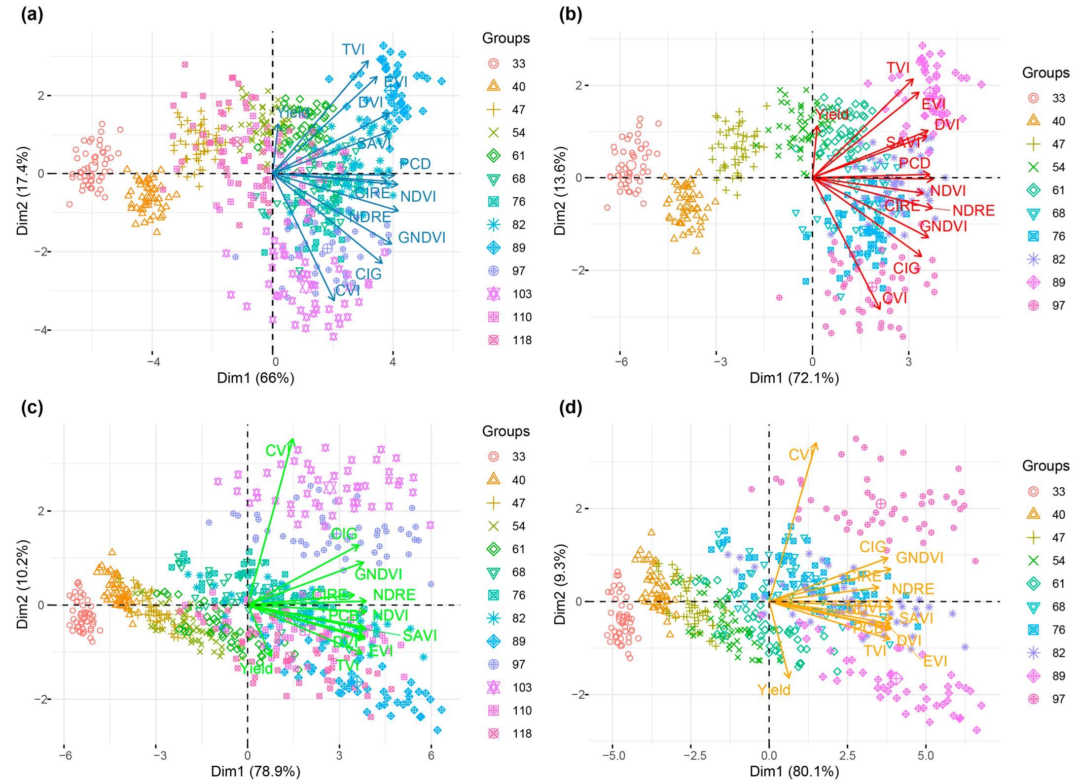
3.5. Multivariate—Principal Components Analysis

The principal component analysis (PCA) for the 13 dates evaluated throughout the vegetative development of beans, with 11 VIs estimated from multispectral images with method 1 (Figure 8a), explained 90.6% of variance with their values. The first two components (Dim1, 72% and Dim2, 18.6%), in which the last three groups in chronological order are widely dispersed, and are not adequately differentiated from the other clusters, for which reason it was proposed that we build another PCA graph in biplot for the first 10 evaluations from 33 to 97 DAS (Figure 7b), which succeeded in explaining 93.2% of the observed variance and would be between stages V4 to R8 of the bean crop phenology [37]. Regarding the variables of the indexes in the PCA, we can observe a great correlation between EVI and TVI (r = 0.98 ***) and between SAVI and DVI (r = 0.79 ***) with 89 DAS (Figure 8a,b). The PCA with the estimated indices of method 2 for the 13 (96.7% of the explained variance) and 10 dates evaluated (97.1% of the explained variance) (Figure 8c,d) showed less clarity in the groupings between the evaluated dates based on these 11 indices, in comparison with the PCA obtained from the estimated indices of method 1. These vegetation indices, based on the reflectance of the canopy for each plot of the four commercial bean cultivars with yields (Figure 9), are a current and practical alternative for crop research and production.

4. Discussion

The yield of a crop depends on the environmental factor, the genetic purity of the seed [38], its interaction with other species and organisms in its environment, the agricultural inputs required and agronomic management. These will influence the yield component to a greater or lesser extent [39]. To forecast yield, new emerging technologies are required, such as geospatial tools for the development of predictive models in agriculture [40]. Unfortunately, these tools have not been widely employed in Peruvian agriculture.

Bean grain yield showed significant differences among cultivars. The camanejo cultivar had the highest yield (2.77 t/ha), and the average yields obtained were higher than the national average of 1.2 t/ha [4]. The planting frames between plants (0.4 m) and planting furrows (0.9 m) were fundamental to the development of a good aerial biomass, thus allowing the accumulation of photosynthates in reserve organs such as bean seeds, as reported by Ferrer-Vilca et al. [41], who obtained 2.71 t/ha with organic fertilizer sources in fertile soils in the Amazonian highlands, in the region of Huánuco. The total irrigation lamina (Lr) applied per treatment was as follows: 327 mm (ETo 120%), 307 mm (ETo 100%), 287 mm (ETo 80%) and 266 mm (ETo 60%). Likewise, there were no significant differences for yield (Figure 2b). These results indicate that the bean crop is highly resistant to water stress during the flowering and ripening stage. Irrigation sheets for the bean crop in arid zones require a volume of 300 to 500 mm as reported by Beebe et al. [42].

The biometric growth variables (plant height and dry biomass) showed a continuous increase, as well as the VIs (Figure 3 and Figure 4, Tables S1 and S2) of the bean cultivars [43,44], as observed for NDVI, GNDVI, NDRE, CIG, PCB and CIRE indices in this work (Figure 4a–g). However, these biometric variables presented low correlation with respect to yield. Likewise, chlorophyll content showed no correlation with yield. This could be due to morphological differences in these cultivars; there are slight changes in time for each phenological stage per cultivar, as indicated by Keles et al. [45], who found the highest correlation of SPAD with yield in the flowering stage, but not in later stages (R² = 0.07 ns).

Two methods (methods 1 and 2) were used (Figures S2 and S3), each with 11 VIs, which allowed us to find different index results for the generation of yield prediction models (Figure 6 and Figure 7). In the vegetative stage, the best model was obtained with method 2, and in the reproductive stage with method 1. These results allowed for a better analysis and interpretation of results on the influence of the soil with respect to the plant canopy, the adequate management of resources and data processing. According to these results, Palaniswami et al. [46] indicated that in remote sensing, it is necessary to delimit or classify the vegetation to eliminate noise within the image; the RGB image allows a better classification of vegetation by grouping identical pixels with the categories of interest of the user, as performed in method 1.

The results of this study showed high correlations (***) between the yield for four cultivars and VIs, during 89 to 118 DAS (Table 2 and Table 3). The models built with data from these four cultivars, both for method 1 and 2, showed maximum R² at 103 and 110 DDS (Figures S6 and S7) using at least five VIs (R² = 0.483 *** and R² = 0.476 ***, respectively). These phenological stages (R8 and R9) correspond to maturity and the beginning of senescence, as shown in Figure 8, the yield map per evaluated plot. Likewise, prediction models were established for the early stages (vegetative and reproductive) per cultivar. Therefore, this research determined the average VIs by the phenological stage in the bean crop and then calculated the correlation (Pearson-r) between the averages VIs (Figure 5) with both methods, showing greater significance and variation between the vegetative (Figure 5a,b), reproductive (Figure 5c,d) and maturity (Figure 5e,f) stages, with the CIRE, DVI, EVI and TVI indices with respect to the other six VIs (NDVI, GNDVI, CIG, NDRE, PCB and SAVI). In method 1 (Figure 5a,c,e), there was no correlation, and they presented Pearson-r values negative or close to zero, while in method 2 (Figure 5b,d,f), they had highly significant correlations, with Pearson-r close to one, showing a clear influence of ground reflectance together with canopy cover on multispectral images for the CVI, CIRE, DVI, EVI and TVI indices. The development of the prediction models for each cultivar by phenological stage allowed us to increase the R² value, reaching the maximum for cultivar c2000 (R² = 0.9424 **) in the vegetative stage with method 1. These indices will allow us to discriminate, with high precision, the phenological stages between cultivars or other study treatments.

The supervised classification for method 1 considers orthomosaic images over the crop canopy, allowing for a better grouping between the dates evaluated in the PCA (Figure 8a,b) with the VIs. This is because it only considers the reflectance of the aerial biomass of the plants [42], mainly at the vegetative growth, maturity (stages V4 to R8) and senescence stages. These analyses were also used in remote sensing studies as reported by Mokarram and Pham [47], who predicted the yield of two species, namely, as palm and pomegranate, by evaluating the effect of drought on yield with NDVI, PCI and VCI VIs. Prudnikova et al. [48] expressed that differences in the global reflectance values of the soils studied are mainly due to variations in their organic matter contents, since they have a similar texture and mineralogical composition, which influences the estimation of the vegetation indices and the reflectivity of crops.

Yield prediction at pre-harvest stages, with traditional methods, is time consuming, subjective and costly. On the other hand, the empirical models are usually limited specifically to the area and the surrounding environment [49] at a local level, and the results obtained may present the most practical and effective method for yield prediction [50] by the cultivar and phenological stages, with very little data collected in the field. However, there are also various machine learning methods, including neural networks, tree ensembles and a kernel method to predict yield crops [51]. The methodologies employed in this work can be applied in the different regions of Peru, where bean cultivars are usually grown.

5. Conclusions

Multispectral UAV imagery was demonstrated to have great potential in the yield estimation of P. vulgaris. In this work, prediction models were developed for four bean cultivars under four irrigation treatments in pre-harvest stages. Results confirmed that the estimation of vegetative indices at different crop stages provided a high degree of correlation with yield with respect to CIG, PCB, DVI, EVI and TVI indices with method 2 for the c2000 cultivar, but when model 1 (NDVI, NDRE, SAVI, CVI and CIRE) and 2 (NDVI, SAVI, CVI, EVI and TVI) were employed at the reproductive stage, a high degree of correlation was obtained for the camanejo cultivar. The models that best predicted bean yield were estimated for the physiological stages, i.e., V3–V4 and R6–R8 (vegetative and reproductive). The principal components for the dates evaluated with the vegetation indices showed a change and increase in the values of the indices according to the vegetative development and phenology of the crop, representing a potential tool by which to discriminate treatments or evaluations of crop management.

References

1. Campos-Vega, R.; Reynoso-Camacho, R.; Pedraza-Aboytes, G.; Acosta-Gallegos, J.A.; Guzman-Maldonado, S.H.; Paredes-Lopez, O.; Oomah, B.D.; Loarca-Piña, G. Chemical Composition and in Vitro Polysaccharide Fermentation of Different Beans (Phaseolus vulgaris L.). J. Food Sci. 2009, 74, T59–T65. [Google Scholar] [CrossRef] [PubMed]
2. Shamseldin, A.; Velázquez, E. The Promiscuity of Phaseolus vulgaris L. (Common Bean) for Nodulation with Rhizobia: A Review. World J. Microbiol. Biotechnol. 2020, 36, 63. [Google Scholar] [CrossRef] [PubMed]
3. Mecha, E.; Figueira, M.; Vaz, M.C.; do Rosário, M. Two Sides of the Same Coin: The Impact of Grain Legumes on Human Health: Common Bean (Phaseolus vulgaris L.) as a Case Study. In Legume Seed Nutraceutical Research; IntechOpen: London, UK, 2019; pp. 26–46. [Google Scholar] [CrossRef]
4. MIDAGRI. Plan Nacional de Cultivos: Campaña Agrícola 2019–2020; MIDAGRI: Lima, Perú, 2020; Available online: https://cdn.www.gob.pe/uploads/document/file/471867/Plan_Nacional_de_Cultivos_2019_2020b.pdf (accessed on 13 November 2022).
5. Shakoor, N.; Lee, S.; Mockler, T.C. High Throughput Phenotyping to Accelerate Crop Breeding and Monitoring of Diseases in the Field. Curr. Opin. Plant Biol. 2017, 38, 184–192. [Google Scholar] [CrossRef] [PubMed]
6. Eggen, M.; Ozdogan, M.; Zaitchik, B.; Ademe, D.; Foltz, J.; Simane, B. Vulnerability of Sorghum Production to Extreme, Sub-Seasonal Weather under Climate Change. Environ. Res. Lett. 2019, 14, 045005. [Google Scholar] [CrossRef]
7. Wijesingha, J.; Dayananda, S.; Wachendorf, M.; Astor, T. Comparison of Spaceborne and UAV-Borne Remote Sensing Spectral Data for Estimating Monsoon Crop Vegetation Parameters. Sensors 2021, 21, 2886. [Google Scholar] [CrossRef]
8. Puntarenas, P.; Rica, C.; Rica, U.D.C.; Rica, C.; Nacional, U.; Rica, C. Caracterización Espectral y Detección de Flecha Seca En Palma Africana En Puntarenas, Costa Rica. Rev. Geográfica Am. Cent. 2018, 2, 329. [Google Scholar] [CrossRef]
9. Gano, B.; Dembele, J.S.B.; Ndour, A.; Luquet, D.; Beurier, G.; Diouf, D.; Audebert, A. Using Uav Borne, Multi-Spectral Imaging for the Field Phenotyping of Shoot Biomass, Leaf Area Index and Height of West African Sorghum Varieties under Two Contrasted Water Conditions. Agronomy 2021, 11, 850. [Google Scholar] [CrossRef]
10. Guo, Y.; Wang, H.; Wu, Z.; Wang, S.; Sun, H.; Senthilnath, J.; Wang, J.; Bryant, C.R.; Fu, Y. Modified Red Blue Vegetation Index for Chlorophyll Estimation and Yield Prediction of Maize from Visible Images Captured by Uav. Sensors 2020, 20, 5055. [Google Scholar] [CrossRef]
11. Han, L.; Yang, G.; Dai, H.; Xu, B.; Yang, H.; Feng, H.; Li, Z.; Yang, X. Modeling Maize Above-Ground Biomass Based on Machine Learning Approaches Using UAV Remote-Sensing Data. Plant Methods 2019, 15, 1–19. [Google Scholar] [CrossRef]
12. Vega, F.A.; Ramírez, F.C.; Saiz, M.P.; Rosúa, F.O. Multi-Temporal Imaging Using an Unmanned Aerial Vehicle for Monitoring a Sunflower Crop. Biosyst. Eng. 2015, 132, 19–27. [Google Scholar] [CrossRef]
13. Yue, J.; Feng, H.; Jin, X.; Yuan, H.; Li, Z.; Zhou, C.; Yang, G.; Tian, Q. A Comparison of Crop Parameters Estimation Using Images from UAV-Mounted Snapshot Hyperspectral Sensor and High-Definition Digital Camera. Remote Sens. 2018, 10, 1138. [Google Scholar] [CrossRef]
14. Mwinuka, P.R.; Mbilinyi, B.P.; Mbungu, W.B.; Mourice, S.K.; Mahoo, H.F.; Schmitter, P. The Feasibility of Hand-Held Thermal and UAV-Based Multispectral Imaging for Canopy Water Status Assessment and Yield Prediction of Irrigated African Eggplant (Solanum aethopicum L.). Agric. Water Manag. 2021, 245, 106584. [Google Scholar] [CrossRef]
15. Parker, T.A.; Palkovic, A.; Gepts, P. Determining the Genetic Control of Common Bean Early-Growth Rate Using Unmanned Aerial Vehicles. Remote Sens. 2020, 12, 1748. [Google Scholar] [CrossRef]
16. Santos, A.F.; Lacerda, L.N.; Rossi, C.; Moreno, L.D.A.; Oliveira, M.F.; Pilon, C.; Silva, R.P.; Vellidis, G. Using UAV and Multispectral Images to Estimate Peanut Maturity Variability on Irrigated and Rainfed Fields Applying Linear Models and Artificial Neural Networks. Remote Sens. 2022, 14, 93. [Google Scholar] [CrossRef]
17. Saravia, D.; Salazar, W.; Valqui-Valqui, L.; Quille-Mamani, J.; Porras-Jorge, R.; Corredor, F.-A.; Barboza, E.; Vásquez, H.V.; Casas Diaz, A.V.; Arbizu, C.I. Yield Predictions of Four Hybrids of Maize (Zea mays) Using Multispectral Images Obtained from UAV in the Coast of Peru. Agronomy 2022, 12, 2630. [Google Scholar] [CrossRef]
18. Quille-Mamani, J.; Porras-Jorge, R.; Saravia-Navarro, D.; Valqui-Valqui, L.; Herrera, J.; Chávez-Galarza, J.; Arbizu, C.I. Assessment of Vegetation Índices Derived from UAV Images for Predicting Biometric Variables in Bean during Ripening Stage. Idesia 2022, 40, 39–45. [Google Scholar] [CrossRef]
19. SENAMHI. Mapa Climático del Perú; SENAMHI: Lima, Peru, 2022; Available online: https://www.senamhi.gob.pe/?p=mapa-climatico-del-peru (accessed on 30 April 2022).
20. Santos, A.E.; Barbosa, M.R.; de Almeida Moreira, B.R.; da Silva, R.P.; Lemos, L.B. UAV Multispectral Data: A Reliable Approach for Managing Phosphate-Solubilizing Bacteria in Common Bean. Agronomy 2022, 12, 2284. [Google Scholar] [CrossRef]
21. Marques, A.P.; Prado, L.; Garcia, D.E.; Nunes, W.; Cordeiro, D.; Ribeiro, L.P.; da Silva, C.A.; Capristo-Silva, G.F.; Li, J.; Rojo, F.E.; et al. A Random Forest Ranking Approach to Predict Yield in Maize with Uav-Based Vegetation Spectral Indices. Comput. Electron. Agric. 2020, 178, 105791. [Google Scholar] [CrossRef]
22. Peñuelas, J.; Gamon, J.A.; Griffin, K.L.; Field, C.B. Assessing Community Type, Plant Biomass, Pigment Composition, and Photosynthetic Efficiency of Aquatic Vegetation from Spectral Reflectance. Remote Sens. Environ. 1993, 46, 110–118. [Google Scholar] [CrossRef]
23. Gitelson, A.A.; Kaufman, Y.J.; Merzlyak, M.N. Use of a Green Channel in Remote Sensing of Global Vegetation from EOS- MODIS. Remote Sens. Environ. 1996, 58, 289–298. [Google Scholar] [CrossRef]
24. Gitelson, A.; Merzlyak, M.N. Quantitative Estimation of Chlorophyll-a Using Reflectance Spectra: Experiments with Autumn Chestnut and Maple Leaves. J. Photochem. Photobiol. B Biol. 1994, 22, 247–252. [Google Scholar] [CrossRef]
25. Pearson, R.L.; Miller, L.D. Remote Mapping of Standing Crop Biomass for Estimation of the Productivity of the Shortgrass Prairie. Remote Sens. Environ. 1972, 1, 1355. [Google Scholar]
26. Huete, A.R. A soil-adjusted vegetation index (SAVI). Remote Sens. Environ. 1988, 25, 295–309. [Google Scholar] [CrossRef]
27. Vincini, M.; Frazzi, E.; D’Alessio, P. A Broad-Band Leaf Chlorophyll Vegetation Index at the Canopy Scale. Precis. Agric. 2008, 9, 303–319. [Google Scholar] [CrossRef]
28. Gitelson, A.A.; Gritz, Y.; Merzlyak, M.N. Relationships between Leaf Chlorophyll Content and Spectral Reflectance and Algorithms for Non-Destructive Chlorophyll Assessment in Higher Plant Leaves. J. Plant Physiol. 2003, 160, 271–282. [Google Scholar] [CrossRef]
29. Duarte, L.; Teodoro, A.C.; Sousa, J.J.; Pádua, L. Qvigourmap: A Gis Open Source Application for the Creation of Canopy Vigour Maps. Agronomy 2021, 11, 952. [Google Scholar] [CrossRef]
30. R Core Team. R: A Language and Environment for Statistical Computing; R Foundation for Statistical Computing: Vienna, Austria, 2021; Available online: https://www.r-project.org/ (accessed on 12 November 2022).
31. R Core Team. RStudio: Integrated Development for R. Rstudio Team; PBC: Boston, MA, USA, 2020; Available online: https://www.rstudio.com/authors/rstudio-team/ (accessed on 4 November 2022).
32. Schloerke, B.; Cook, D.; Larmarange, J.; Briatte, F.; Marbach, M.; Thoen, E.; Elberg, A.; Crowley, J. Package “GGally”. Available online: https://cran.r-project.org/web/packages/GGally/GGally.pdf (accessed on 12 November 2022).
33. Wickham, H. ggplot2: Elegant Graphics for Data Analysis, 2nd ed.; Springer: Cham, Switzerland, 2016. [Google Scholar]
34. de Mendiburu, F. Package “Agricolae”. Available online: https://cran.r-project.org/web/packages/agricolae/agricolae.pdf (accessed on 5 November 2022).
35. Kassambara, A.; Mundt, F. Package “Factoextra”. Available online: https://cran.r-project.org/web/packages/factoextra/factoextra.pdf (accessed on 12 November 2022).
36. Lê, S.; Josse, J.; Husson, F. FactoMineR: An R Package for Multivariate Analysis. J. Stat. Softw. 2008, 25, 1–18. [Google Scholar] [CrossRef]
37. Rosales-Serna, R.; Flores-Gallardo, H.; López-González, J.C.; Rubiños-Panta, J.E.; Ortiz-Sánchez, I.A.; Flores-Magdaleno, H.; Santana-Espinoza, S.; Domínguez-Martínez, P.A. Fenología y Productividad Del Agua En Variedades Mejoradas de Frijol Pinto Cultiva-Das En Durango, México. Rev. Fitotec. Mex. 2021, 44, 511. [Google Scholar] [CrossRef]
38. Kumar, R.; Gupta, A. Seed-Borne Diseases of Agricultural Crops: Detection, Diagnosis & Management; Springer: Berlin/Heidelberg, Germany, 2020; pp. 1–871. [Google Scholar] [CrossRef]
39. Grassini, P.; Thorburn, J.; Burr, C.; Cassman, K.G. High-Yield Irrigated Maize in the Western U.S. Corn Belt: I. On-Farm Yield, Yield Potential, and Impact of Agronomic Practices. Field Crop. Res. 2011, 120, 142–150. [Google Scholar] [CrossRef]
40. Sishodia, R.P.; Ray, R.L.; Singh, S.K. Applications of Remote Sensing in Precision Agriculture: A Review. Remote Sens. 2020, 12, 3136. [Google Scholar] [CrossRef]
41. Ferrer-Vilca, T.H.; Valverde-Rodríguez, A. Rendimiento del frejol (Phaseolus vulgaris L.) variedad canario con tres fuentes de abonos orgánicos en el distrito de Cholón, Huánuco-Perú. Rev. Investig. Agrar. 2020, 2, 33–44. [Google Scholar] [CrossRef]
42. Beebe, S.; Ramirez, J.; Jarvis, A.; Rao, I.M.; Mosquera, G.; Bueno, J.M.; Blair, M.W. Genetic Improvement of Common Beans and the Challenges of Climate Change; John Wiley & Sons: Oxford, UK, 2011; pp. 356–369. [Google Scholar]
43. Jeong, C.H.; Park, J.H. Analysis of Growth Characteristics Using Plant Height and NDVI of Four Waxy Corn Varieties Based on UAV Imagery. Korean J. Remote Sens. 2021, 37, 733–745. [Google Scholar] [CrossRef]
44. Gebremedhin, A.; Badenhorst, P.; Wang, J.; Giri, K.; Spangenberg, G.; Smith, K. Development and Validation of a Model to Combine NDVI and Plant Height for High-Throughput Phenotyping of Herbage Yield in a Perennial Ryegrass Breeding Program. Remote Sens. 2019, 11, 2494. [Google Scholar] [CrossRef]
45. Keles, R.; Bayrak, H.; Imriz, G. Determination of Grain Yield and Leaf Chlorophyll Content of Some Dry Bean (Phaseolus vulgarıs L.) Varieties. J. Glob. Innov. Agric. Soc. Sci. 2019, 7, 53–57. [Google Scholar] [CrossRef]
46. Palaniswami, C.; Upadhyay, A.K.; Maheswarappa, H.P. Spectral Mixture Analysis for Subpixel Classification of Coconut. Curr. Sci. 2006, 91, 1706–1711. [Google Scholar]
47. Lipovac, A.; Bezdan, A.; Moravčevic, D.M.; Djurovic, N.; Cosic, M.; Benka, P.; Stričevic, R.S. Correlation between Ground Measurements and UAV Sensed Vegetation Indices for Yield Prediction of Common Bean Grown under Different Irrigation Treatments and Sowing Periods. Water 2022, 14, 3786. [Google Scholar] [CrossRef]
48. Prudnikova, E.; Savin, I.; Vindeker, G.; Grubina, P.; Shishkonakova, E.; Sharychev, D. Influence of soil background on spectral reflectance of winter wheat crop canopy. Remote Sens. 2019, 11, 1932. [Google Scholar] [CrossRef]
49. Ali, A.M.; Abouelghar, M.; Belal, A.A.; Saleh, N.; Yones, M.; Selim, A.I.; Amin, M.E.S.; Elwesemy, A.; Kucher, D.E.; Maginan, S.; et al. Crop Yield Prediction Using Multi Sensors Remote Sensing (Review Article). Egypt. J. Remote Sens. Sp. Sci. 2022, 25, 711–716. [Google Scholar] [CrossRef]
50. dela Torre, D.M.G.; Gao, J.; Macinnis-Ng, C. Remote Sensing-Based Estimation of Rice Yields Using Various Models: A Critical Review. Geo-Spat. Inf. Sci. 2021, 24, 580–603. [Google Scholar] [CrossRef]
51. Nyéki, A.; Kerepesi, C.; Daróczy, B.; Benczúr, A.; Milics, G.; Nagy, J.; Harsányi, E.; Kovács, A.J.; Neményi, M. Application of Spatio-Temporal Data in Site-Specific Maize Yield Prediction with Machine Learning Methods. Precis. Agric. 2021, 22, 1397–1415. [Google Scholar] [CrossRef]
Figure 1. Location of the study area the La Molina Experimental Center in Lima (Peru).
Drones 07 00325 g001
Figure 2. Means comparison with Duncan test (alpha = 0.05) for the yield of the four bean cultivars (a) and the irrigation treatments evaluated in the experiment (b). Groups with means plus standard deviation. ns. p-value > 0.05, * p-value < 0.05, ** p-value < 0.01 and *** p-value < 0.001. Red triangles are each data collected.
Drones 07 00325 g002
Figure 3. Evaluations for plant height (a), chlorophyll content SPAD (b) and dry aerial biomass (c) for all bean cultivars in different DAS.
Drones 07 00325 g003
Figure 4. Evaluations for vegetation indices (NDVI (a), GNDVI (b), NDRE (c), CIG (d), PCB (e), SAVI (f), CIRE (g), CVI (h), DVI (i), EVI (j) and TVI (k)) estimated by multispectral images from UAV for all bean cultivars in different DAS.
Drones 07 00325 g004
Figure 5. Pearson-r correlation between all commercial cultivar bean yields with VIs for vegetative (a,b), reproductive (c,d) and ripening (e,f) stages for method 1 (a,c,e) and method 2 (b,d,f) of multispectral images analysis.
Drones 07 00325 g005
Figure 6. Yield evaluated in the field and prediction models for yield of four commercial bean cultivars with multiple linear regression with VIs for the vegetative state of its phenology (33–47 DAS) with supervised classification (with s.c.) for method 1 (ac) and method 2 (df) of the analysis of multispectral images. ns. p-value > 0.05, * p-value < 0.05, ** p-value < 0.01 and *** p-value < 0.001.
Drones 07 00325 g006
Figure 7. Yield evaluated in the field and prediction models for yield of four commercial bean cultivars with multiple linear regression with VIs for the reproductive stae of its phenology (54 at 68 DAS) with supervised classification (with s.c.) for method 1 (ac) and method 2 (df) of the analysis of multispectral images. ns. p-value > 0.05, * p-value < 0.05, ** p-value < 0.01 and *** p-value < 0.001.
Drones 07 00325 g007
Figure 8. PCA Biplot graph of the multivariate analysis of the main components for the 13 (a) and 10 (b) dates evaluated (DAS) with the VIs in all commercial bean cultivars and with method 1 and method 2 (c,d) of the analysis of multispectral images.
Drones 07 00325 g008
Figure 9. Yield map according to each plot in the experimental field, where plot 101 (1, 2, 3 and 4) corresponds with irrigation treatments and the sub-plot (101_1, 101_2, 101_3 and 101_4) (48 unit) corresponds with four commercial bean cultivars.
Drones 07 00325 g009