Repeated UAV Observations and Digital Modeling for Surface Change Detection in Ring Structure Crater Margin in Plateau

Abstract

As UAV technology has been leaping forward, small consumer-grade UAVs equipped with optical sensors are capable of easily acquiring high-resolution images, which show bright prospects in a wide variety of terrains and different fields. First, the crater rim landscape of the Dinosaur Valley ring formation located on the central Yunnan Plateau served as the object of the surface change detection experiment, and two repetitive UAV ground observations of the study area were performed at the same altitude of 180 m with DJI Phantom 4 RTK in the rainy season (P1) and the dry season (P2). Subsequently, the UAV-SfM digital three-dimensional (3D) modeling method was adopted to build digital models of the study area at two points in time, which comprised the Digital Surface Model (DSM), Digital Orthomosaic Model (DOM), and Dense Image Matching (DIM) point cloud. Lastly, a quantitative analysis of the surface changes at the pit edge was performed using the point-surface-body surface morphological characterization method based on the digital model. As indicated by the results, (1) the elevation detection of the corresponding check points of the two DSM periods yielded a maximum positive difference of 0.2650 m and a maximum negative value of −0.2279 m in the first period, as well as a maximum positive difference of 0.2470 m and a maximum negative value of −0.2589 m in the second period. (2) In the change detection of the two DOM periods, the vegetation was 9.99% higher in the wet season than in the dry season in terms of coverage, whereas the bare soil was 10.54% more covered than the wet season. (3) In general, the M3C2-PM distances of the P1 point cloud and the P2 point cloud were concentrated in the interval (−0.2,0.2), whereas the percentage of the interval (−0.1,0) accounted for 26.69% of all intervals. The numerical model of UAV-SfM was employed for comprehensive change detection analysis. As revealed by the result of the point elevation difference in the constant area, the technique can conform to the requirements of earth observation with certain accuracy. The change area suggested that the test area can be affected by natural conditions to a certain extent, such that the multi-source data can be integrated to conduct more comprehensive detection analysis.

1. Introduction

As unmanned aerial vehicle (UAV) technology has been advancing rapidly, small consumer-grade UAVs equipped with optical sensors are capable of easily acquiring high-resolution images, which are promising in different fields (e.g., geology [1], physical geography [2], and topographic and geomorphological [3] analysis).

Structure from Motion (SfM) has been confirmed as the main technical method of aerial survey digital image processing, i.e., UAV-SfM serves as the core technology for the in-depth research on consumer-grade UAV technology in areas (e.g., landslides, geology, and geomorphology). Moreover, UAV-SfM is building increasingly rich digital models with time. In the planar dimension, i.e., two-dimensional (2D) digital models comprise Digital Orthophoto Map (DOM) and Digital Elevation Model (DEM), and so forth. In the stereoscopic dimension, i.e., in three dimensions, the data models involve realistic models and Dense Image Matching (DIM) point clouds. Numerous scholars have adopted the UAV-SfM method in different fields to develop models and conduct relevant experimental analyses. To be specific, Ilinca et al. [4] carried out digital image acquisition based on DJI Phantom 4 and Phantom 4 RTK UAVs in the village of Livadea, Romania, and then built a digital model for landslide detection in the experimental area using the UAV-SfM algorithm. As revealed by the results, the average displacement of the entire landslide reaches 20 m. The efficiency of the UAV-SfM technique is confirmed when a rapid response and measures are required to reduce the consequences of a landslide with serious hazards. Marques et al. [5] built digital images as a DOM using the UAV-SfM technique, focusing on fracture detection in karst areas. Cho et al. [6] used the UAV-SfM technique to monitor displacement of steep slopes, so as to reduce unexpected losses due to slope failures. Vollgger et al. [7] built a DOM and Digital Surface Model (DSM) from aerial survey data using UAV-SfM. Gomez et al. [8] conducted UAV digital image acquisition and LiDAR point cloud acquisition of the annual Merapi volcanic dome in 2012 and 2014, respectively. Additionally, they employed the LiDAR point cloud and the UAV-SfM. As indicated by the results, the evolution of the crater rim around the dome has been generally stable between 2012 and 2014, i.e., no large-scale collapse has occurred. Furthermore, it is explained in the outlook that the experiment only conforms to the DEM for monitoring comparisons, and comparative analyses can be attempted based on point clouds for data from multiple periods.

In addition, the relevant numerical models built by the UAV-SfM technique in different topographic and geomorphological environments (e.g., plains, dunes, and basins) are capable of meeting a certain level of accuracy. To be specific, Vecchi et al. [9] applied Global Navigation Satellite System (GNSS) and UAV-SfM techniques in the shoreline area and showed that there was a difference of ±10 cm between the point elevation of GNSS and DSM in the test area. Qian et al. [10] sought for a more accurate and efficient measurement method in the dune area. In accordance with the 3D data and DOM acquired from UAV images, they examined the dune morphological parameters based on DJI Phantom4 RTK in the crescent-shaped dune area of the Qaidam Basin. As indicated by the results, a good correlation existed between the 2D and 3D morphologies of this dune area, and the conversion of 2D remote sensing image measurement results to 3D parameters (e.g., dune height and dune volume) can be achieved, which can provide a useful reference for efficient and accurate modeling of the dune area. Zhang et al. [11] verified the accuracy of digital terrain data from consumer-grade UAVs, set an aerial height of 50 m in 10 m steps with a maximum aerial height of 100 m, and acquired UAV image data from a standard experimental site in the Soil and Water Conservation Park in Yanqing County, Beijing through six aerial heights to produce digital terrain models (e.g., densely matched image point clouds, DSMs, and DOMs). The accuracy was verified using Global Positioning System (GPS) examined checkpoints. As revealed by the results, the average errors of the digital terrain models reached ±0.51 cm and ±4.39 cm in the horizontal and vertical directions, respectively. Gao et al. [12] combined UAV aerial survey techniques to build a high-precision DOM and DEM for extracting information on complex alluvial fan tectonic activity in the Balikun Basin, Xinjiang. The digital model built by the UAV-SfM technique is capable of accurately identifying the location of active faulted steep sides and detecting the remains of alluvial fan tectonic deformation. Clapuyt et al. [13] examined the plain area by UAV while changing the focal length of the camera and the position of the georeferenced target between flights. A comparison of the numerical models built by UAV-SfM suggested that errors were controlled within centimeters based on the control variables method.

Digital products built with UAV-SfM technology have been extensively employed in different industry sectors and terrains, and the accuracy has been verified by many scholars from various aspects. Yu et al. [14] examined the elevation accuracy of the DSM and point cloud models built by UAV-SfM through ground checkpoints. Gao et al. [15] used UAV-SfM technology to build DSM and DOM in a plateau urban area and performed DSM point level and elevation change detection. As indicated by the results, UAV-SfM can control the level accuracy and vertical accuracy in centimeter range in this test area. Barba et al. [16] evaluated the model accuracy of UAV-SfM in Avella (Italy), a Roman amphitheater at an archaeological site. Moreover, they confirmed the significance of a good geo-reference for digital models, using sufficient and evenly distributed checkpoints to verify quality. A careful analysis of the point cloud should also be conducted to obtain high quality and reliable products. Farella et al. [17] registered the point cloud built by UAV-SfM with the LiDAR point cloud, conducted filtering processing, and detected the point cloud using the cloud-to-cloud method. Mousavi et al. [18] proposed a Multi-Criteria Decision Making (MCDM) automatic filtering method for the experiment, which is presented for the accuracy increase of the UAV-SfM built model for point cloud models in different regions.

In brief, many domestic and foreign researchers and scholars have studied and detected the UAV-SfM built DOM, DSM, and point cloud models of the studied area in different fields and different terrains, whereas the existing analysis has only been from a single perspective (e.g., point and 3D point cloud or two perspectives of point and surface). As revealed by the above analysis of the current situation, UAV-SfM technology has become increasingly mature, whereas the comprehensive detection of digital models obtained using the UAV-SfM method has been rarely investigated, especially in the highland mountainous areas where the terrain is relatively more complex. Thus, the UAV image data were collected in this study at the pit rim of the plateau ring mountain area, and the digital model built by UAV-SfM was adopted to detect the changes of point and surface in the 2D digital model from the perspective of point elements and surface elements defined by geographic entities [19]. Next, the feasibility of the digital model built by the UAV-SfM method was verified by the difference of the invariant area in the highland and complex terrain. Moreover, the perspective of the body elements defined for the geographic entities [20] in the 3D digital model in terms of direct cloud-to-cloud comparison with closest point technique (C2C) [21], absolute distance, and James et al. [22] in Multiscale Model to Model Cloud Comparison (M3C2) was based on the proposed M3C2-PM distance for the DIM point cloud body change detection. The UAV-SfM digital model point-surface-body all-round change detection was adopted to analyze the changes in the highland cratonic mountains.

2. Research Method

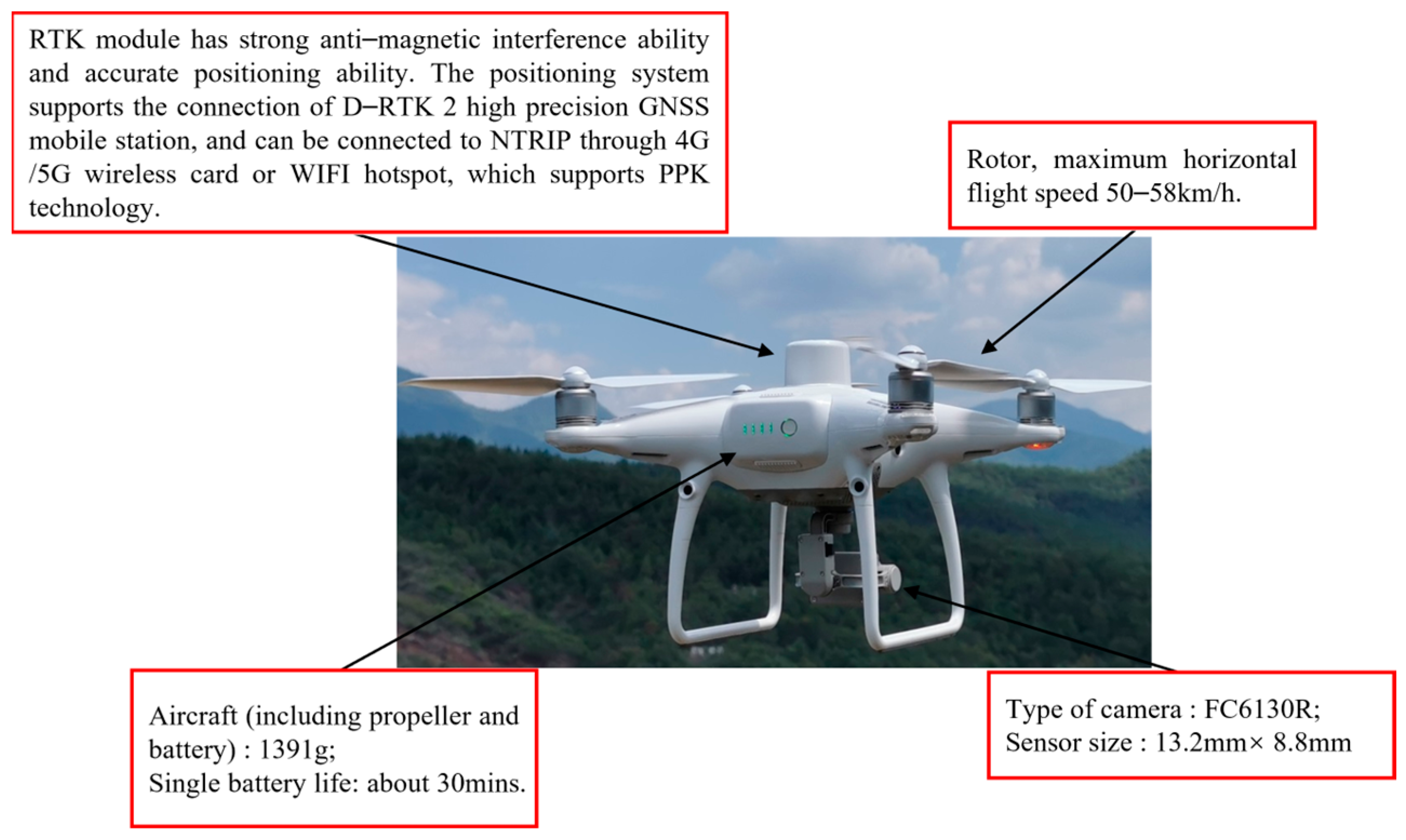
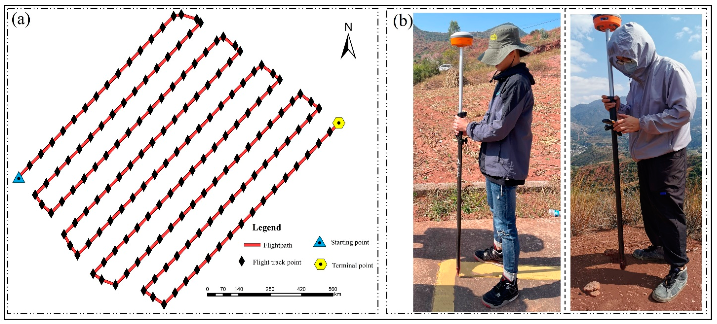
2.1. Test Area and Data Collection

The study area is located in the mountainous region of the southern rim of the Dinosaur Valley in Lufeng County, Chuxiong Yi Autonomous Prefecture, Yunnan Province, and Figure 1a presents its approximate location in the administrative region. The geomorphological types in the survey area are complex and diverse, dominated by erosional landforms and square mountain landforms. It is characterized by a sub-hot, low-latitude highland monsoon climate with two distinct dry and wet seasons. Weeds and low shrubs are primarily distributed in the test area under the effect of the geological conditions and climatic environment. Due to the existence of small Mesozoic red sedimentary basins in the test area, soil types are distributed in bands, and purple and red soils are widely distributed, with the scene presented in Figure 1b. Based on the 12.5 m low-resolution DEM of the test area downloaded from ALOS in Tuxin Cloud GIS, the profiles were drawn in four directions (i.e., from north to south, northeast to southwest, west to east, as well as northwest to southeast) in accordance with the four lines in Figure 1b. The profiles are presented in Figure 1c, the entire cratered mountain area rises and falls, whereas the elevations of the entrance and exit locations in the four directions are highly variable relative to the interior of the cratered mountain area. On that basis, the northeastern pit rim in the area was selected. The entrance area, represented by the red line in Figure 1b, was adopted to capture UAV images of this area and conduct detailed change detection analysis of the associated 2D and 3D digital models.

This application of DJI Phantom 4 RTK is oriented to collect UAV low-altitude images in the mountainous region of the southern rim of Dinosaur Valley. The vehicle was released by DJI Innovation Technology Ltd., Shenzhen, China in June 2018, equipped with a high-performance imaging system and a high-precision navigation and positioning system in a lightweight body. The RTK module is capable of receiving single-frequency GNSS and multi-frequency multi-system high precision RTK GNSS, such that the positioning accuracy of the data collected by the UAV in the highland mountains can be ensured to a certain extent (Figure 2).

Table 1. UAV platform and camera parameters.

UAV Platform		Camera Params
Type	DJI Phantom 4 RTK	Type	FC6310R
Maximum area for a single flight	0.7 km2	Sensor size	13.2 mm × 8.8 mm
Hover time	60 min	Photo size	5472 × 3648/pixel
Highest working altitude	1850 km	Pixel size	2.41 μm
Maximum flight rate	12 m/s	Camera focal length	8.8 mm

lists the parameters of the aircraft and lens sensor. The original observation values recorded by the RTK module and the camera instant exposure data can be determined by PPK using DJI cloud PPK technology or integrated ground base station data. Accordingly, the difficulty of aerial survey can be reduced, and the efficiency of aerial survey can be improved to a certain extent.

UAV route planning significantly affects image quality and subsequent product accuracy. Before data collection, a field survey should be performed in the experimental area. According to the actual terrain conditions and relevant aerial survey requirements, reasonable design should be made for ground sampling distance, relative navigation height, side direction and course overlap degree, and navigation height can be determined by Equation (1):

$$H=\frac{f\times GSD}{\alpha }$$

(1)

where $H$ denotes the relative navigation height, affecting the size of the image. In complex terrain areas, route height should be appropriately increased in accordance with the situation. ƒ represents the focal distance of the camera, which can be queried in the introduction of its parameters. $GSD$ is the ground sampling distance, and the smaller the value, the higher the accuracy of aerial survey. $\alpha$ is the pixel size.

Digital image data acquisition was performed via DJI Phantom 4 RTK, with images of the two areas collected in July and November 2022, with a four-month interval between data collection periods. Figure 3a presents the route of the test area, and the flight height for the UAV acquisition data are determined as 180 m by Equation (1). Given that the vehicle comes with its own RTK, the position information is recorded in real time through the Thousand Seeker account at the UAV operation. Moreover, RTK is used to collect checkpoint information in a uniform distribution over the test area (Figure 3b).

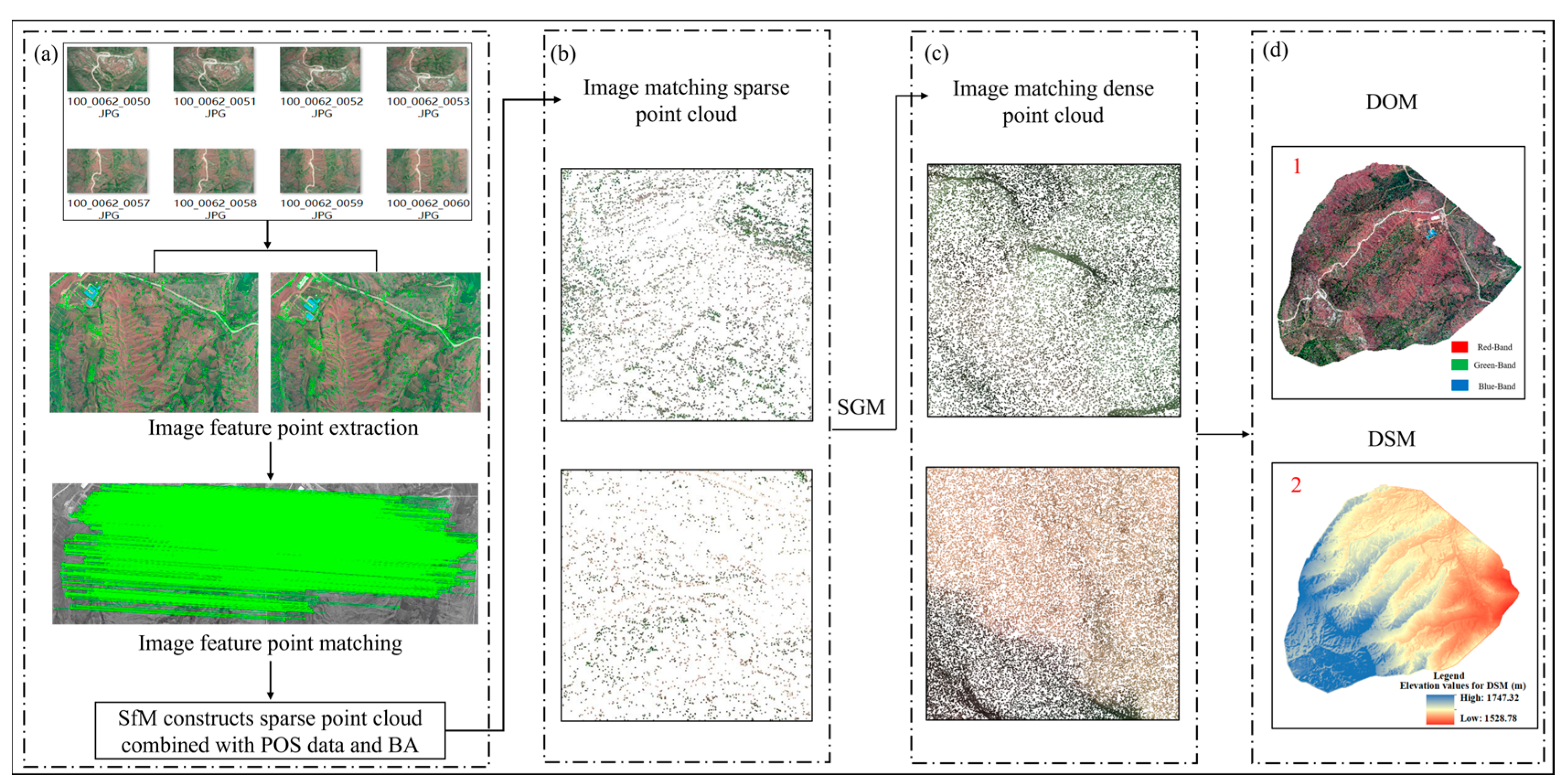
2.2. UAV Digital Model Building Techniques

First, for UAV digital model construction, to obtain a point cloud by dense matching of images, the collected data are removed from images with obscuring features (e.g., low-flying birds, fog, and smoke). Subsequently, the image feature points are extracted and matched. With the SfM algorithm, the aim is to find the right camera and scene parameters to optimize the objective of solving the sparse image matching point cloud from the image by matching the features and satisfying the required image pairs, and initializing the image pairs with a single-strain model. Through Random Sample Consensus (RANSAC) algorithm for image noise reduction processing, after using the five-point method to determine the outer orientation elements of the initialized matching image pair, the trajectory triangulation image pair for Bundle Adjustment (BA) is present (Figure 4a).

Second, all points in the point cloud are projected onto the respective image, the corresponding point and pixel coordinates are found, and the BA iteration is completed. When using SfM to solve the image, the POS data should be combined with a certain number of ground control points for feature extraction and matching of the image, and an aerial triangulation based on the beam method area network leveling model should be conducted to connect the ground coordinates and accurately solve the inner and outer orientation elements to obtain a sparse 3D point cloud (Figure 4b).

Next, sparse point cloud is based on the PhotoScan platform and a semi-global matching algorithm (SGM) [23] similar to that used to build the image dense point cloud is applied. Its energy function is given by Equation (2). The minimum is the global energy optimization strategy to find the optimal parallax for the respective pixel. The basic process is mainly performed in four steps, i.e., cost matching calculation, cost aggregation, parallax calculation, and parallax refinement, and the solved dense point cloud is illustrated in Figure 4c.

Lastly, the texture information is mapped to a dense point cloud to build the DOM and DSM, both with a spatial resolution of 7 cm (Figure 4d):

$$E(D)=E_{data}(D)+E_{smooth}(D)$$

(2)

where $E_{data}$ denotes data item, represents the overall matching cost measure; $E_{smooth}$ is a smooth term, making the parallax reach the condition constraint.

DIM point clouds refer to a major digital model produced by UAV aerial survey technology, generated from images with high overlap, and are used in areas such as agriculture and forestry, power line inspection and topographic mapping, containing both true color information and 3D coordinate and attribute information of feature points. Moreover, DIM point clouds contain the following four characteristics that make them rapidly popular in various industries [24]:

(1) Lower costs, easier operation of equipment, and relatively higher efficiency compared to 3D laser scanner equipment;

(2) Contains not only 3D coordinate information, but also rich spectral and texture information, which greatly reduces the difficulty of subsequent processing;

(3) Does not have echo intensity, and for features such as vegetation and buildings does not have the ability to collect surface data directly compared to LiDAR point clouds;

(4) Due to the presence of features, the DIM point cloud generates the DSM directly, but a series of processes are also applied to the point cloud to obtain a DEM that accurately describes the surface information.

2.3. UAV Technical Framework for Quantification of Repeated Observation Errors

Digital models (e.g., DOM, DSM, and DIM point clouds) can be obtained by digitizing UAV aerial survey images. The experiment of this study takes a 2D point and surface perspective, and in three dimensions with a body perspective, the UAV aerial survey digital model is oriented towards the detection of surface changes at different points in the crater rim of the Dinosaur Valley South Rim, as illustrated in the process shown in Figure 5.

DSM contains the geographical information of the test area while covering the elevation information and texture information of different features on the surface. Using Equation (3) [25], the elevation values extracted from the two phases of the DSM were determined by the error of 60 points collected by RTK, and the elevation change of the surface information of the crater rim of the Dinosaur Valley South Rim is analyzed by the difference:

$$D_i=Q_i-Q_{ture}$$

(3)

where $Q_i$($i=1,2$) represents the image construction DSM in July and November, $Q_i$ represents the RTK collection of 60 checkpoint values, and $D_i$ represents the difference.

For the Support Vector Machines (SVM) algorithm, many scholars have applied it to classify remote sensing images with a certain guarantee of classification accuracy [26,27]. The same SVM method is used in this study for DOM classification. SVM is used mainly to learn the way of sample nonlinear $N_i$ mapping $\theta$ to high-dimensional kernel function space $\beta$, as shown in Equation (4). The optimal hyperplane is then built based on the high-dimensional feature space, as in Equation (5). $N_i$ refers to any set of sample data values, as expressed in Equation (6). By constructing and using different kernel functions, the SVM algorithm builds the discriminant function by finding the dot product of the vectors and performing a non-linear transformation to the inner product in the high-dimensional feature space for the solution, instead of by mapping the sample data set directly into the high-dimensional feature space for the solution set:

$$\theta :R^m\to \beta$$

(4)

$$\omega ·N_i+a=0$$

(5)

$$N_i:\left\{\left(N_1,Y_1\right),\left(N_2,Y_2\right)\dots \left(N_i,Y_i\right)\right\},N\in R^m,Y\in \left(-1,1\right)$$

(6)

where $\omega$ and $a$ denotes constant (excluding 0), $i$ is the number of samples, and $m$ represents the dimension of high-dimensional feature space.

The optimal classification plane is built in $\beta$, whose inner product defines the kernel function according to Equation (7), which can replace the dot product operation in the optimal plane and transfer the sample data set to the new feature space, where the optimization function is defined by Equation (8). Decision functions, as in Equation (9), support vectors, and intermediate nodes corresponding to each other can be output by linear combination of intermediate nodes:

$$K\left(x_i,x_j\right)=\phi (x_i)·\phi (x_j)$$

(7)

$$L_D(\partial )={\displaystyle \sum _{i=1}^m{\partial }_i-\frac{1}{2}{\displaystyle \sum _{i,j=1}^m{\partial }_i{\partial }_j{y}_i}}{y}_{j}K(x_i,x_j)$$

(8)

$$f(x)=sign({\displaystyle \sum _{i=1}^m{\partial }_i{y}_{i}K(x_i,x_j)-a})$$

(9)

where ${\partial }_i{\partial }_j$ and $y_i{y}_j$ denote the coefficient that goes into Lagrange, and $a$ can be determined in accordance with ${\partial }_i\left\{y_i\left(\left(\omega ·x_i\right)-a\right)-1\right\}=0, i=0,1,2\dots m$.

High-density point clouds allow for the construction of refinement to build live 3D models and digital terrain models, whereas the time taken by the computer increases linearly with the rise of the point cloud density. Moreover, the objective of point cloud refinement is to meet the point cloud in the process of converting it to the rest of the digital product. This study places a focus on the application of octree [28] for point cloud refinement, where the space falls into 2n × 2n × 2n sub-cubes by a circular recursive method in the structural division of the octree. Thus, the respective node corresponds to a cube and each cube contains eight sub-cubes, and the side lengths of the sub-cubes are the side lengths of the previous level along the x-direction, y-direction, and half of the z-direction of the node cube. The segmentation was continuously performed on all nodes and stops when the number of 3D points contained in a node is less than or equal to the set minimum number of points contained in the cube. After the segmentation subdivision, point cloud refinement was completed in the partitioned mesh by the location of the points in the center.

The point cloud refined by the octree algorithm was quantified by point-to-point, point-to-surface, and body-to-body change errors to enable quantitative analysis of 3D digital model change detection of UAV at the crater rim of a highland crater ring. The main methods include: (1) C2C [21]; (2) Distance between the point cloud and the reference 3D grid or theoretical model which is used to obtain the surface displacement (cloud-to-mesh distance or cloud-to-model distance, C2M) [29], and (3) M3C2 [30]. To be specific, C2C calculates the distance difference of point cloud by calculating the distance between the point in P1 point cloud and the nearest point in P2 point cloud, as shown in Figure 6a. C2M is to build P1 point cloud as a grid, P1a as a reference grid point, and then each discrete point in P2 point cloud. With P2a as an example, the distance between the two points is adopted to obtain the distance difference of point cloud, as shown in Figure 6b.

M3C2 has the following features: (1) it does not need to grid or raster the point cloud, and can be directly determined in the point cloud model; (2) As the local distance of the normal vector surface between two point clouds is determined, the 3D changes of the surface can be directly detected during the calculation of this algorithm.

In the M3C2 algorithm, the distance between the local average point cloud models is determined by the selected points in the reference point cloud. For each core point a, the direction $Z$ of the local surface normal is determined by fitting the plane to all its adjacent points in a distance of $\frac{H}{2}$, as presented in the first step of Figure 6c. Then, the local surface position of the respective point cloud is determined into the average position of the cylinder, where $h$ expresses the diameter of the bottom circle. Additionally, along the normal direction $Z$ (the second step of Figure 6c), the distance of the respective point in point cloud $\mathrm{P}1$ and $\mathrm{P}2$ is given. The position of point cloud is shown as $\mathrm{P}{1}_a$ and $\mathrm{P}{2}_a$, and the distance is ${\mathrm{D}}_{\mathrm{M}3\mathrm{C}2}$. For P1 point clouds and P2 point clouds, the M3C2 algorithm uses the local rough in the core point along the normal direction Z as a measure of the uncertainty of the average position between the point clouds, so as to measure the accurate confidence interval (LoD) of the distance.

However, the errors in coordinate measurement of the respective point of UAV-SfM point cloud are highly correlated with the errors in adjacent points. Aiming at the characteristics of UAV-SfM point cloud, James et al. [22] proposed the M3C2-PM algorithm on the basis of M3C2. By using the M3C2 algorithm, the local normal vector distance is also determined. Furthermore, the M3C2 algorithm is adjusted to be suitable for UAV-SfM point cloud in combination with 3D accuracy estimation of a correlation accuracy map, as shown in the third step of Figure 6c. The accuracy values (in units X, Y, and Z) are determined in the mapping between point pairs of $\mathrm{P}{1}_a$ and $\mathrm{P}{2}_a$. The accuracy estimates are associated and represent error ellipsoids. LoD 95% can be estimated by combining the precision components ${\sigma }_1$ and ${\sigma }_2$ of the local surface normal vector direction, as shown in Equation (10):

$$Lo{D}_{95\%}\left(h\right)=\pm 1.96\left(\sqrt{{\sigma }_1{}^2+{\sigma }_2{}^2}\right)+reg$$

(10)

where $reg$ denotes the relative population registration error between measurements, assuming isotropy and uniform space, and $reg$ represents the potential systematic deviation. Under the identical aerial geographic coordinate system of ${\sigma }_1$ and ${\sigma }_2$, $reg$ is zero. Therefore, a non-zero value can be adopted in accordance with the actual situation. The output of M3C2-PM indicates the change between point clouds along the local normal direction, as well as the local LoD 95% value of whether the change exceeds the change in the 3D space of the point cloud and the geographical registration accuracy of UAV-SfM.

3. Test Results and Analysis

3.1. Two Phases of DSM Point Surface Change Detection Results and Analysis

Remote sensing image change detection can rapidly determine changes in land types, while it can also be adopted to estimate disasters (e.g., floods and forest fires). Moreover, the 2D digital model of UAV saves manpower and resources in acquiring data, and it is efficient and accurate at the data processing and interpretation stages [31]. The elevation values of the two DSMs were extracted to check points at the identical location, and Figure 7a presents the point distribution. Subsequently, the difference between the DSMs were determined, and Figure 7b presents the results. The difference between P1-DSM is represented as a red line in the figure, and the calculation results fell into a scope of ±0.3 m, where the maximum positive difference was 0.2650 m, and the maximum negative difference reached −0.2279 m. A blue line in the figure represents the difference between P2-DSM. The difference between the DSM extracted elevation values and the examined points was relatively higher in the rainy and dry seasons than in the dry season due to the scouring of the mountain by rain.

3.2. Two Phases of DOM Surface Change Detection Results and Analysis

The experiment of this study was oriented towards the detection of facet changes in a 2D digital model of the crater rim of the plateau ring, and the faceted geoid information was extracted from two phases of a high-resolution DOM based on the eCognition platform.

First, the local variance of the segmented objects were determined, and the LV-ROC curve was generated to determine the suitable segmentation scale for the experiment. Next, the sample points were selected in accordance with the five categories of bare soil, bare rock, vegetation, roads, and buildings for training by the SVM method. Moreover, two phases of DOM classification tests were completed on the trained data, where shrubs, weeds, and crops were classified as vegetation. Lastly, the global accuracy (OA) and Kappa coefficient of SVM classification were determined [32].

The OA in the classification P1-DOM reached 92.14%, and the Kappa coefficient was 90.38%, whereas the OA in the classification P2-DOM was 91.54% and the Kappa coefficient was 90.53% (Figure 8). Statistical information on the facets of the land classification is presented in Figure 8a for classification, P1-DOM, with bare soil, bare rock, vegetation, roads, and buildings accounts for 42.48%, 5.75%, 50.19%, 1.16%, and 0.42% of the total number of objects classified, respectively. Figure 8b presents the classification P2-DOM with bare soil, bare rock, vegetation, roads, and buildings accounting for 53.02%, 5.34%, 40.20%, 1.02%, and 0.42% of the total number of objects classified, respectively. The test area is characterized by a wet and dry climate, with the first phase data collected during the rainy season, covering the largest area of vegetation, 9.99% over the second phase data, and the second phase data collected in the dry season, covering the largest area of bare soil, 10.54% more than the first phase data. In addition to the crops on the cultivated land, i.e., the result of anthropogenic changes in land type, the low vegetation (e.g., weeds and shrubs on both sides of the mountain) were affected by the natural factors of the monsoon climate of the subtropical low-latitude plateau, resulting in an increase in the extent of bare soil cover in the test area in the dry season.

Except for vegetation and bare soil, the ground cover of buildings did not change. However, the clam-over scope of the road has changed, mainly because the main soil types in the test area are red soil and purple soil, and the soil viscosity is low, which is easy to cause landslides on the side of the road when washed by rain, resulting in partial accumulation of silt on the road. The change area is shown in Figure 9a. It is shown in the red line segment. Moreover, the inspection points were taken in the road area, and the elevation values in the two phases of DSM were extracted for difference. The difference values were shown in Figure 9b. The maximum point difference in the road area was 0.05 m in the inspection points, and the minimum value was close to 0. Some road areas are misclassified as bare soil in SVM classification. The variation of the two land species in the rainy and dry seasons conforms to the objective law, which can be reflected from the changes of the 2D information content of the UAV’s 2D digital model, excluding natural factors. The 2D digital model built by DJI Phantom 4 RTK aerial survey images in the plateau ring mountain region can indicate that the UAV can meet certain precision measurement requirements from the perspective of surface change information detection $\left(x,y\right)$, and the perspective of checkpoint difference from the region between 0 and 0.05 m $\left(z\right)$.

3.3. Two Phases of DIM Point Cloud Bulk Surface Change Detection Results and Analysis

In the LiDAR360 platform, the DIM point cloud of P1 and P2 was streamlined, and the selection range of octree was from 1 to 21. There was a linear correlation between the number of trees and the number of reserved points, and the smaller the number, the fewer the number of reserved points. Thus, the point cloud of P1 was taken as an example first, with 3 as the step length, and the number of octrees decreased from 21 to carry out the point cloud (Figure 10). The octree decreased slowly in the first three thresholds. However, when the octree number changed from 15 to 12, the number of point clouds decreased from tens of millions to millions; when the threshold varied from 12 to 9, the number of point clouds declined from millions to 100,000. To ensure that the threshold setting of octree quantity can better conform to the requirements of point cloud simplification, 8 was taken as the threshold to try, only 55,383 point clouds were retained, and the overall contour features of the test area were lost, such that the subsequent threshold value was not tested.

To better balance the correlation between computing time and accuracy of the subsequent point clouds, the number of octrees was reduced to 1 as a step, and the point clouds of both phases were streamlined in the octree number range of 14 to 9.

Table 2. 3D deviation analysis results of different threshold values.

Point Cloud Simplification	Number of Octree	Number of Point Clouds	Max Positive Distance (mm)	Max Negative Distance (mm)	Mean Positive Deviation (mm)	Mean Negative Deviation (mm)	Standard Deviation (mm)
P1	14	11,429,372	6.7108	−4.2862	0.0211	−0.0267	0.0349
	13	11,236,415	8.2580	−6.4234	0.0322	−0.0359	0.0483
	12	8,848,073	12.1168	−7.5916	0.0254	−0.0302	0.0679
	11	3,152,781	6.7203	−11.2484	0.0386	−0.0394	0.0797
	10	858,742	29.2274	−9.4400	0.0906	−0.0852	0.1684
	9	220,736	5.9734	−10.6810	0.1970	−0.1927	0.2792
P2	14	11,346,632	0.2214	−0.2111	0.0213	−0.0226	0.0344
	13	11,183,022	0.1617	−0.1653	0.0240	−0.0289	0.0372
	12	8,117,006	3.1165	−1.3441	0.0295	−0.0332	0.0433
	11	2,855,882	0.4111	−4.4794	0.0431	−0.0465	0.0660
	10	856,353	1.0998	−6.3910	0.1018	−0.1052	0.1429
	9	224,668	7.5991	−9.5990	3.3294	−2.3203	0.4573

lists in the P1 and P2 point clouds, respectively at octree 11, the number of P1 point clouds was 3,152,787, the standard deviation reached 0.0797 mm, and the number of P2 point clouds was 2,855,882, the standard deviation reached 0.0660 mm, both in the order of one million. Moreover, the point clouds were effectively streamlined.

In accordance with the P1 point cloud, the streamlined point clouds of 15, 11, and 9 were selected and compared with the original point cloud. First, the global features of the respective point cloud were extracted, i.e., the contour range of the whole test area. Subsequently, the area and perimeter of the extracted range were calculated (Figure 11). The original point cloud took up an area of 0.7293 km², and the perimeter was 4.340 km. The refined point cloud with an octree of 11 took up an area of 0.7286 km², and the perimeter was 4.307 km, marking the reduction of 0.0007 km² and 0.037 km, respectively. The building information in the yellow box of the point cloud with an octree of 11 was partially distorted compared with the building information in the yellow box of the point cloud with an octree of 15, while it is better preserved compared to the building information in the point cloud with an octree of 9. The global and local features of the point cloud can illustrate the validity of this experiment of streamlining the point cloud with an octree of 11.

The point cloud model change interpretation of UAV can simultaneously judge the relevant areas of ground object change from multiple perspectives, that is, interpret the change area by means of body change. Based on CloudCompare, for 3,152,781 point clouds of P1 and 2,855,882 point clouds of P2, the C2C algorithm is used to obtain the absolute distance of the two models according to the maximum distance. The results are shown in Figure 12a. The absolute distance of surface point cloud C2C in the test area is concentrated below 2.5 m. The change area between 1 m and 2.5 m is mainly concentrated in the point cloud edge region shown in Figure 12c and crop growth region shown in Figure 12d.

To ensure that the surface roughness is not interfered with by vegetation, buildings, and other ground objects, the M3C2-PM algorithm needs to eliminate the obvious ground object area [33,34]. Through 2D–3D mapping, vegetation area and building area are eliminated, and point clouds P1 and P2 are classified as ground points according to attribute classification. According to the terrain elements, the step size was set as 10 cm, starting from 0 to the initial value of 2.5 m, the appropriate normal vector fitting radius was selected, and the maximum depth was adjusted to 0.4 m by referring to the actual situation. The core point cloud was adjusted with P1 point cloud and P2 point cloud respectively, and the elimination method was used to select P1 point cloud as the core point cloud, and the normal vector was determined in the vertical direction. The M3C2-PM algorithm was used to detect the volume changes of point clouds in P1 and P2 phases and obtain the results. As shown in Figure 13a, the M3C2-PM distance of point clouds in P1 and P2 is normally distributed. To accurately analyze the M3C2-PM distance of P1 point cloud and P2 point cloud, the percentage of point cloud in each distance segment in the total determined amount was counted according to the horizontal axis interval. As depicted in Figure 13b, $\left[0.5,0.6\right]$ segment only accounted for 0.019%, and $\left[-0.1,0\right)$ segment accounted for the highest with 26.69%. The proportion of $\left[0,0.1\right)$ interval was 21.97%, and the interval higher than 10% was mainly concentrated in $\left[-0.2,0.2\right]$ interval.

The M3C2-PM distance of P1 and P2 point clouds mainly concentrated in the interval $\left[-0.2,0.2\right]$ was converted into a grid, and mountain shadow and ridgeline were superimposed to finely interpret the 3D digital model changes of the UAV (Figure 14). As indicated by visual interpretation, the changes on both sides of the blue and red lateral ridgelines were significant. The M3C2-PM distance changes on both sides of J1 and J4 were mainly in the interval $\left[0,0.2\right]$, whereas the changes on the right side of J2 were primarily in the interval $\left[-0.2,0\right]$. The M3C2-PM distance variation on both sides of J3 was more significant than that on other longitudinal ridgelines, especially in the intersection area of two ridgelines. J5 represents the transverse ridgeline, and the low vegetation in the right area has been removed from the point cloud in the 2D–3D mapping. Accordingly, the change of M3C2-PM distance was mainly in the left pit area, and the positive change turned out to be relatively more significant.

The digital model is capable of accurately expressing the morphological characteristics of the landscape. The process of soil erosion, sediment transport, and runoff in the mountainous areas of the plateau can be clearly explained through the interpretation of the point-line-surface-body elements of the micro-landscape features. Numerous scholars have studied the morphological characteristics of micro-landscapes as terraces, low-lying flatlands, isolated depressions, combined depressions, and slopes [35,36], and the morphological characteristics are presented in Figure 15a. With reference to this micro-geomorphological feature, the 3D digital model change area of the experiment of this study can be classified as sloping land. Using the UAV digital model to finely interpret the topographic features of the micro-land formation types in the highland ring mountains to analyze the changes in the morphological features of the mountains caused by natural factors in the region is the main work to follow. Figure 15b, 1, and 2 were field photographs taken during the P1 point cloud and P2 point cloud periods, respectively. Combined with the fieldwork, the area was dominated by red loam and purple soils, which were affected by natural factors such as rainfall and wind erosion, and the area was markedly depressed by footsteps after rainfall during the rainy season, and the red loam and purple soils were severely sanded during the dry season.

4. Results and Discussion

4.1. Results

In this study, a DJI Phantom 4 RTK consumer-grade UAV was employed for data acquisition, and the UAV was combined with the UAV-SfM method to build 2D and 3D UAV digital models of the entrance to the crater rim of the Central Yunnan Plateau by using the control variables method and repeated observations at different points in the wet and dry seasons at 180 m aerial height.

As revealed by the results of the point and surface variation in the 2D digital model, i.e., DSM and DOM, in terms of point and surface elements defined for geographical entities:

(1) The results of the spatial analysis of the P1-DSM, P2-DSM, and checkpoints to accurately obtain the elevation differences fell into the scope of ±0.3 m.

(2) Bare soil, bare rock, vegetation, roads, and buildings accounted for 42.48%, 5.75%, 50.19%, 1.16%, and 0.42% of the total number of classified objects in the P1-DOM, respectively, whereas the five categories of land in the P2-DOM accounted for 53.02%, 5.34%, 40.20%, 1.02%, and 0.42%, respectively;

As indicated by the results, the C2C absolute distance of the surface point cloud in the test area was concentrated below 2.5 m, and the M3C2-PM distances of the P1 and P2 point clouds were mainly concentrated in the interval [−0.2,0.2], whereas the highest percentage accounted for 26.69% in the interval [−0.1,0) and the second highest reached 21.97% in the interval [0,0.1).

4.2. Discussion

DJI Phantom 4 RTK consumer drone was adopted to build a digital model for the UAV-SfM technology in the highland ring of mountains, and in the 2D surface change detection in the rainy and dry seasons, mainly vegetation and bare soil areas. The vegetation cover was 9.99% higher in the wet season than in the dry season, whereas the bare soil cover was 10.54% higher in the dry season. The M3C2-PM distances detected in the 3D body digital model change were mainly distributed on both sides of the vertical and horizontal ridgelines. Moreover, in combination with the field survey, purple soils, and red soils on both sides of the ridge were sandy in the dry season. To fully apply the UAV-SfM technology to interpret the topography of the area and analyze the causes, the next step of the study will be to integrate multi-source remote sensing data and combine rainfall, soil, and biological factors to analyze the situation in the test area in detail.

5. Conclusions

A comprehensive change detection analysis of the UAV-SfM digital model was performed to detect point and face changes in the 2D digital model from the perspective of point and face elements defined as geographic entities. The DSM detects point errors, the DOM detects face change information, and the body change detection was performed in the 3D DIM point cloud. In the experiment of this study, points were randomly selected in the face change detection area of the 2D DOM, and the elevation values were extracted from the two DSM phases to the same point. Subsequently, the difference between the points in the area was generated, and the elevation difference between the check points in the area ranged from 0 to 0.05 m, suggesting that the DJI Phantom 4 RTK is capable of conforming to the requirements of ground observation in the highland. As revealed by the above result, the DJI Phantom 4 RTK can conform to the requirements of ground observation with a certain degree of accuracy in the mountainous region of the ring, and the quality of the data is ensured to a certain extent, such that a solid foundation is laid for the subsequent processing of a wide variety of models.

The change in elevation turned out to be more prominent in the rainy season than in the dry season with the 2D DSM, the surface change detection of the DOM was affected by the season, and the main change categories comprised bare soil and vegetation. Moreover, the change areas on both sides of the ridge were indicated by the change detection in the 3D DIM point cloud. The UAV-SfM technique can be combined with other technical means and information for the in-depth validation and analysis of the causes of changes in the mountains affected by natural conditions.

References

1. Uzkeda, H.; Poblet, J.; Magan, M.; Bulnes, M.; Martin, S.; Fernandez-Martinez, D. Virtual outcrop models: Digital techniques and an inventory of structural models from North-Northwest Iberia (Cantabrian Zone and Asturian Basin). J. Struct. Geol. 2022, 157, 104568–104585. [Google Scholar] [CrossRef]
2. He, H.; Ye, H.; Xu, C.; Liao, X. Exploring the Spatial Heterogeneity and Driving Factors of UAV Logistics Network: Case Study of Hangzhou, China. ISPRS Int. J. Geo-Inf. 2022, 11, 419. [Google Scholar] [CrossRef]
3. Hussain, Y.; Schlogel, R.; Innocenti, A.; Hamza, O.; Iannucci, R.; Martino, S.; Havenith, H.B. Review on the Geophysical and UAV-Based Methods Applied to Landslides. Remote Sens. 2022, 14, 4564. [Google Scholar] [CrossRef]
4. Ilinca, V.; Șandric, I.; Chițu, Z.; Irimia, R.; Gheuca, I. UAV applications to assess short-term dynamics of slow-moving landslides under dense forest cover. Landslides 2022, 19, 1717–1734. [Google Scholar] [CrossRef]
5. Marques, A.; Racolte, G.; Zanotta, D.C.; Menezes, E.; Cazarin, C.L.; Gonzaga, L.; Veronez, M.R. Adaptive Segmentation for Discontinuity Detection on Karstified Carbonate Outcrop Images From UAV-SfM Acquisition and Detection Bias Analysis. IEEE Access 2022, 10, 20514–20526. [Google Scholar] [CrossRef]
6. Cho, J.; Lee, J.; Lee, B. Application of UAV Photogrammetry to Slope-Displacement Measurement. KSCE J. Civ. Eng. 2022, 26, 1904–1913. [Google Scholar] [CrossRef]
7. Vollgger, S.A.; Cruden, A.R. Mapping folds and fractures in basement and cover rocks using UAV photogrammetry, Cape Liptrap and Cape Paterson, Victoria, Australia. J. Struct. Geol. 2016, 85, 168–187. [Google Scholar] [CrossRef]
8. Gomez, C.; Setiawan, M.A.; Listyaningrum, N.; Wibowo, S.B.; Suryanto, W.; Darmawan, H.; Bradak, B.; Daikai, R.; Sunardi, S.; Prasetyo, Y.; et al. LiDAR and UAV SfM-MVS of Merapi Volcanic Dome and Crater Rim Change from 2012 to 2014. Remote Sens. 2022, 14, 5193. [Google Scholar] [CrossRef]
9. Vecchi, E.; Tavasci, L.; De Nigris, N.; Gandolfi, S. GNSS and Photogrammetric UAV Derived Data for Coastal Monitoring: A Case of Study in Emilia-Romagna, Italy. J. Mar. Sci. Eng. 2021, 9, 1194. [Google Scholar] [CrossRef]
10. Qian, G.Q.; Yang, Z.L.; Dong, Z.B.; Tian, M. Three-dimensional Morphological Characteristics of Barchan Dunes Based on Photogrammetry with A Multi-rotor UAV. J. Desert Res. 2019, 39, 18–25. [Google Scholar]
11. Zhang, C.B.; Yang, S.T.; Zhao, C.S.; Lou, H.Z.; Zhang, Y.C.; Bai, J.; Wang, Z.W.; Guan, Y.B.; Zhang, Y. Topographic data accuracy verification of small consumer UAV. J. Remote Sens. 2018, 22, 185–195. [Google Scholar]
12. Gao, S.P.; Ran, Y.K.; Wu, F.Y.; Xu, L.X.; Wang, H.; Liang, M.J. Using UAV photogrammetry technology to extract information of tectonic activity of complex alluvial fan—A case study of an alluvial fan in the southern margin of Barkol basin. Seismol. Geol. 2017, 39, 793–804. [Google Scholar]
13. Clapuyt, F.; Vanacker, V.; Van Oost, K. Reproducibility of UAV-based earth topography reconstructions based on Structure-from-Motion algorithms. Geomorphology 2016, 260, 4–15. [Google Scholar] [CrossRef]
14. Yu, J.J.; Kim, D.W.; Lee, E.J.; Son, S.W. Determining the Optimal Number of Ground Control Points for Varying Study Sites through Accuracy Evaluation of Unmanned Aerial System-Based 3D Point Clouds and Digital Surface Models. Drones 2020, 4, 49. [Google Scholar] [CrossRef]
15. Gao, S.; Gan, S.; Yuan, X.P.; Bi, R.; Li, R.B.; Hu, L.; Luo, W.D. Experimental Study on 3D Measurement Accuracy Detection of Low Altitude UAV for Repeated Observation of an Invariant Surface. Processes 2021, 10, 4. [Google Scholar] [CrossRef]
16. Barba, S.; Barbarella, M.; Di Benedetto, A.; Fiani, M.; Gujski, L.; Limongiello, M. Accuracy Assessment of 3D Photogrammetric Models from an Unmanned Aerial Vehicle. Drones 2019, 3, 79. [Google Scholar] [CrossRef] [Green Version]
17. Farella, E.M.; Torresani, A.; Remondino, F. Refining the Joint 3D Processing of Terrestrial and UAV Images Using Quality Measures. Remote Sens. 2020, 12, 2837. [Google Scholar] [CrossRef]
18. Mousavi, V.; Varshosaz, M.; Rashidi, M.; Li, W.L. A New Multi-Criteria Tie Point Filtering Approach to Increase the Accuracy of UAV Photogrammetry Models. Drones 2022, 6, 413. [Google Scholar] [CrossRef]
19. Xi, D.P.; Jiang, W.P. Research on 3D Modeling of Geographic Features and Integrating with Terrain Model. Bull. Surv. Mapp. 2011, 4, 23–25. [Google Scholar]
20. Wang, L.; Guo, G.J.; Liu, Y. Structuring methods of geographic entities towards construction of smart cities. Bull. Surv. Mapp. 2022, 2, 20–24. [Google Scholar] [CrossRef]
21. Huang, H.; Ye, Z.H.; Zhang, C.; Yue, Y.; Cui, C.Y.; Hammad, A. Adaptive Cloud-to-Cloud (AC2C) Comparison Method for Photogrammetric Point Cloud Error Estimation Considering Theoretical Error Space. Remote Sens. 2022, 14, 4289. [Google Scholar] [CrossRef]
22. James, M.R.; Robson, S.; Smith, M.W. 3-D uncertainty-based topographic change detection with structure-from-motion photogrammetry: Precision maps for ground control and directly georeferenced surveys. Earth Surf. Process. Landf. 2017, 42, 1769–1788. [Google Scholar] [CrossRef]
23. Yan, L.; Fei, L.; Chen, C.H.; Ye, Z.Y.; Zhu, R.X. A Multi-View Dense Image Matching Method for High-Resolution Aerial Imagery Based on a Graph Network. Remote Sens. 2016, 8, 799. [Google Scholar] [CrossRef] [Green Version]
24. Dong, Y.Q.; Zhang, L.; Cui, X.M.; Ai, H.B. An improved progressive triangular irregular network densification filtering method for the dense image matching point clouds. J. China Univ. Min. Technol. 2019, 48, 459–466. [Google Scholar] [CrossRef]
25. Gao, S.; Yuan, X.P.; Gan, S.; Yang, M.L.; Hu, L.; Luo, W.D. Experimental analysis of spatial feature detection of the ring geomorphology at the south edge of Lufeng Dinosaur Valley based on UAV imaging point cloud. Bull. Geol. Sci. Technol. 2021, 40, 283–292. [Google Scholar] [CrossRef]
26. Keshtkar, H.; Voigt, W.; Alizadeh, E. Land-cover classification and analysis of change using machine-learning classifiers and multi-temporal remote sensing imagery. Arab. J. Geosci. 2017, 10, 1813–1838. [Google Scholar] [CrossRef]
27. Ai, Z.T.; An, R.; Lu, C.H.; Chen, Y.H. Mapping of native plant species and noxious weeds to investigate grassland degradation in the Three-River Headwaters region using HJ-1A/HSI imagery. Int. J. Remote Sens. 2020, 41, 1813–1838. [Google Scholar] [CrossRef]
28. Fang, F.; Chen, X.J. A Fast Data Reduction Method for Massive Scattered Point Clouds Based on Slicing. Geomat. Inf. Sci. Wuhan Univ. 2013, 38, 1353–1357. [Google Scholar]
29. Barnhart, T.B.; Crosby, B.T. Comparing Two Methods of Surface Change Detection on an Evolving Thermokarst Using High-Temporal-Frequency Terrestrial Laser Scanning, Selawik River, Alaska. Remote Sens. 2013, 5, 2813–2837. [Google Scholar] [CrossRef] [Green Version]
30. Lague, D.; Brodu, N.; Leroux, J. Accurate 3D comparison of complex topography with terrestrial laser scanner: Application to the Rangitikei canyon (N-Z). ISPRS J. Photogramm. Remote Sens. 2013, 82, 10–26. [Google Scholar] [CrossRef] [Green Version]
31. Gong, Y.L.; Yan, L. Building Change Detection Based on Multi-Level Rules Classification with Airborne LiDAR Data and Aerial Images. Spectrosc. Spectr. Anal. 2015, 35, 1325–1330. [Google Scholar]
32. Mao, X.G.; Hou, J.Y.; Bai, X.F.; Fan, W.Y. Multiscale Forest Gap Segmentation and Object-oriented Classification Based on DOM and LiDAR. Trans. Chin. Soc. Agric. Mach. 2017, 48, 152–159. [Google Scholar]
33. DiFrancesco, P.M.; Bonneau, D.; Hutchinson, D.J. The Implications of M3C2 Projection Diameter on 3D Semi-Automated Rockfall Extraction from Sequential Terrestrial Laser Scanning Point Clouds. Remote Sens. 2020, 12, 1885. [Google Scholar] [CrossRef]
34. Meng Hout, R.; Maleval, V.; Mahe, G.; Rouvellac, E.; Crouzevialle, R.; Cerbelaud, F. UAV and LiDAR Data in the Service of Bank Gully Erosion Measurement in Rambla de Algeciras Lakeshore. Water 2020, 12, 2478–2506. [Google Scholar]
35. Zhou, F.B.; Liu, X.J. Research on the Automated Classification of Micro-land form Based on Grid DEM. J. Wuhan Univ. Technol. 2008, 2, 172–175. [Google Scholar]
36. Zhou, F.B.; Zou, L.H.; Liu, X.J.; Meng, F.Y. Micro Landform Classification Method of Grid DEM Based on Convolutional Neural Network. Geomat. Inf. Sci. Wuhan Univ. 2021, 46, 1186–1193. [Google Scholar]
Figure 1. General situation of test area: (a) indicates the approximate location of the test area in the administrative area; (b) indicates a live image of the test area; (c) test area profile.
Drones 07 00298 g001
Figure 2. DJI Phantom 4 RTK General.
Drones 07 00298 g002
Figure 3. Course track and checkpoint measurement: (a) UAV data collection routes; (b) RTK actual point locations.
Drones 07 00298 g003
Figure 4. DIM point cloud construction process: (a) Image feature point extraction matching and SfM; (b) sparse 3D point cloud; (c) dense point cloud; (d) DOM and DSM.
Drones 07 00298 g004
Figure 5. Technical process of quantification of repeated observation error of UAV digital model.
Drones 07 00298 g005
Figure 6. Point cloud detection methods: (a) C2C method; (b) C2M method; (c) M3C2 method.
Drones 07 00298 g006
Figure 7. Elevation checkpoint distribution and checkpoint difference: (a) overview of checkpoint distribution; (b) DSM and checkpoint difference between the two phases.
Drones 07 00298 g007
Figure 8. DOM faceted landform: (a) P1-DOM land class; (b) P2-DOM land class.
Drones 07 00298 g008
Figure 9. Outline of the difference in elevation of points in the changed and unchanged areas of the road: (a) outlining the changed area of the road; (b) the difference in elevation of points in the unchanged area.
Drones 07 00298 g009
Figure 10. Correlation between initial threshold and point cloud cover of octrees.
Drones 07 00298 g010
Figure 11. Global and local features of the P1 point cloud: (a) global and local features of the P1-Original point cloud; (b) global and local features of the P1-Octree number 15 streamlined point cloud; (c) global and local features of the P1-Octree number 11 streamlined point cloud; (d) global and local features of the P1-Octree number 11 streamlined point cloud.
Drones 07 00298 g011
Figure 12. C2C absolute distances and local analysis: (a) absolute distances determined by the statistical C2C algorithm for both models; (b) C2C calculation results; (c) point cloud edge areas determined by C2C; (d) crop areas determined by C2C.
Drones 07 00298 g012
Figure 13. M3C2-PM distance and interval proportion statistics: (a) Statistics of point cloud distances determined by the M3C2-PM algorithm; (b) percentage of intervals for point cloud distances determined by the M3C2-PM algorithm.
Drones 07 00298 g013
Figure 14. M3C2-PM local distance and terrain feature analysis.
Drones 07 00298 g014
Figure 15. Micro-geomorphic morphological characteristics and field survey shooting: (a) Micro-geomorphological features; (b) actual photographs of the test area at the time of data collection in both phases.
Drones 07 00298 g015