Article

Estimating Landslide Surface Displacement by Combining Low-Cost UAV Setup, Topographic Visualization and Computer Vision Techniques

by
Vasil Yordanov
1,*,
Quang Xuan Truong
2 and
Maria Antonia Brovelli
1
1
Department of Civil and Environmental Engineering (DICA), Politecnico di Milano, Piazza Leonardo da Vinci 32, 20133 Milan, Italy
2
Information Technology Faculty, Hanoi University of Natural Resources and Environment, 41A Phu Dien Road, Phu Dien, North-Tu Liem District, Hanoi 100000, Vietnam
*
Author to whom correspondence should be addressed.
Drones 2023, 7(2), 85; https://doi.org/10.3390/drones7020085
Submission received: 3 January 2023 / Revised: 17 January 2023 / Accepted: 25 January 2023 / Published: 27 January 2023
(This article belongs to the Special Issue Drones for Natural Hazards)

Abstract

:
Many techniques are available for estimating landslide surface displacements, whether from the ground, air- or spaceborne. In recent years, Unmanned Areal Vehicles have also been applied in the domain of landslide hazards, and have been able to provide high resolution and precise datasets for better understanding and predicting landslide movements and mitigating their impacts. In this study, we propose an approach for monitoring and detecting landslide surface movements using a low-cost lightweight consumer-grade UAV setup and a Red Relief Image Map (a topographic visualization technique) to normalize the input datasets and mitigate unfavourable illumination conditions that may affect the further implementation of Lucas–Kanade optical flow for the final displacement estimation. The effectiveness of the proposed approach in this study was demonstrated by applying it to the Ruinon landslide, Northern Italy, using the products of surveys carried out in the period 2019–2021. Our results show that the combination of different techniques can accurately and effectively estimate landslide movements over time and at different magnitudes, from a few centimetres to more than several tens of meters. The method applied is shown to be very computationally efficient while yielding precise outputs. At the same time, the use of only free and open-source software allows its straightforward adaptation and modification for other case studies. The approach can potentially be used for monitoring and studying landslide behaviour in areas where no permanent monitoring solutions are present.

Graphical Abstract

1. Introduction

Landslides are considered one of the most devastating geohazards, causing significant damage and loss of life. Accurate and timely monitoring of landslide motion is critical for studying and predicting their possible behavior, as well as to further define suitable mitigating measures to lessen their impact. The growing interest in using remote sensing technologies in recent years is evident in many fields, as technologies such as air- and spaceborne sensors provide invaluable and insightful datasets with constantly increasing capabilities from the spatial, temporal and spectral perspectives [1]. In the context of satellite-based sensing and the domain of landslide hazards, many new approaches and methodologies have been developed and implemented around high-to-medium resolution optical multispectral missions [2,3,4] and weather-invariant radar sensors [5,6], where the main applications are related to mapping historical events, monitoring active and potential slopes [7,8,9], as well as susceptibility mapping and hazard assessment.
Similarly, there is increasing interest in the use of Unmanned Aerial Vehicles (UAV) for landslide studies [10], as UAVs offer several advantages over traditional monitoring methods, including the ability to collect high-resolution imagery, to access difficult-to-reach areas, and to collect data frequently and at a lower cost [11,12]. Therefore, it is natural for scholars to adopt and further exploit this technology also for landslide time-series monitoring [13,14], mapping and characterization [15,16,17] as well as combining their outputs with machine learning [18] and computer vision algorithms [19,20].
For the estimation of landslide surface changes through UAV flyovers, scholars have traditionally used straightforward techniques, such as measuring the difference between Digital Surface Model (DSM) elevation products from consecutive surveys (see [12,16,21,22]) or the direct difference between point clouds (e.g., [11]), which usually results in the quantification of volumetric changes. Such approaches are usually powerful when the landslide under investigation exhibits significant and abrupt changes, however, for some smaller changes and displacements, they can be less efficient, as most of the time alignment error between two products is introduced [23,24], which makes their estimation more difficult. At the same time, scholars have mostly been utilizing high-precision positioning tools for the computation of apparent velocities (e.g., [21,24], which is not always feasible due to the specifics of a terrain. A notable issue in the literature is often related to uneven weather conditions, illumination conditions in particular [20,21,24], which mostly affects the final products from the surveys and then the analyses. Therefore, in the current work, we propose an approach that aims to tackle most of the issues affecting precise surface displacement estimation.
One of the challenges in using UAV-derived imagery for landslide monitoring lies in accurately measuring the apparent surface displacement of the landslide body over time. One solution is using computer vision techniques such as optical flow algorithms [20]. Optical flow algorithms can estimate the motion of objects or features in a sequence of images or videos by tracking the movement of pixels between images/frames and computing the apparent motion of those pixels [25]. The Lucas–Kanade [26] optical flow algorithm is a widely used method that is based on the assumption of small or constant pixel intensity changes between frames. In fact, the latter can cause reconstruction issues and further erroneous displacement estimations when applied in a time-series manner for landslide monitoring, mainly due to unfavorable illumination conditions [19,20] that may occur in one or more epochs. Such conditions are related to different sun directions, shadows and cloud cover, all factors that directly influence image brightness and contrast, i.e., that can further alter the algorithm if directly applied to orthorectified imagery.
An approach for resolving similar issues and ensuring a consistent image intensity is to input normalized products from the UAV surveys. An alternative to the use of orthomaps could be the implementation of a Red Relief Image Maps (RRIM) [27] on three-dimensional data, with photogrammetric products such as DSM derived from UAV surveys. RRIM is a topographic visualization technique, and an alternative to hillshading, which can more successfully highlight morphologic features. The visualization relies on topographic openness [28] and a red-colored slope gradient, and has already been adopted in various studies (e.g., [29,30]).
In this study, we propose a method for monitoring and estimating landslide surface displacements using the products of time-series surveys with a low-cost, consumer-grade UAV and the derived photogrammetric products, such as Digital Surface Models, to which the Red Relief Image Map visualization technique combined with the Lucas–Kanade optical flow algorithm was applied in order to estimate the displacement of pixels between images. The proposed approach allows the measurement of landslide surface motion in 2D space. The effectiveness of this method is demonstrated by applying it to the Ruinon landslide in Northern Italy using datasets from surveys carried out in the period 2019–2021. Processing is done using entirely free and open-source software, which broadens the possibility of adoption and reproducibility. Our method can potentially improve our understanding of landslide behavior and contribute to the development of effective risk mitigation actions in locations where they are lacking.

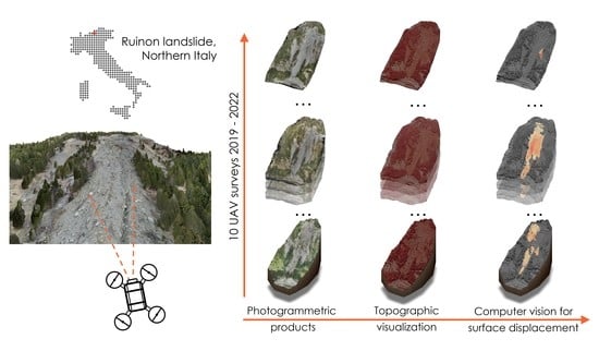
2. Materials and Methods

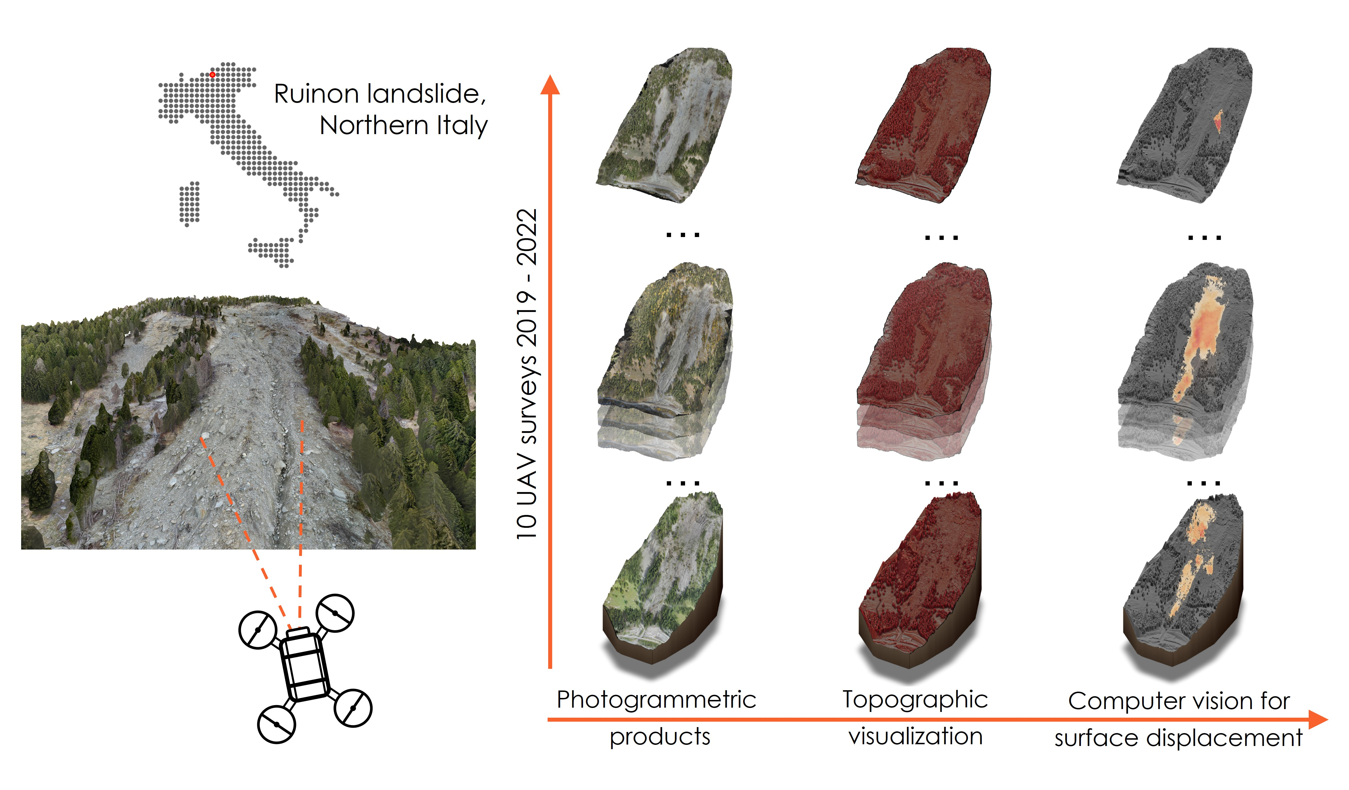
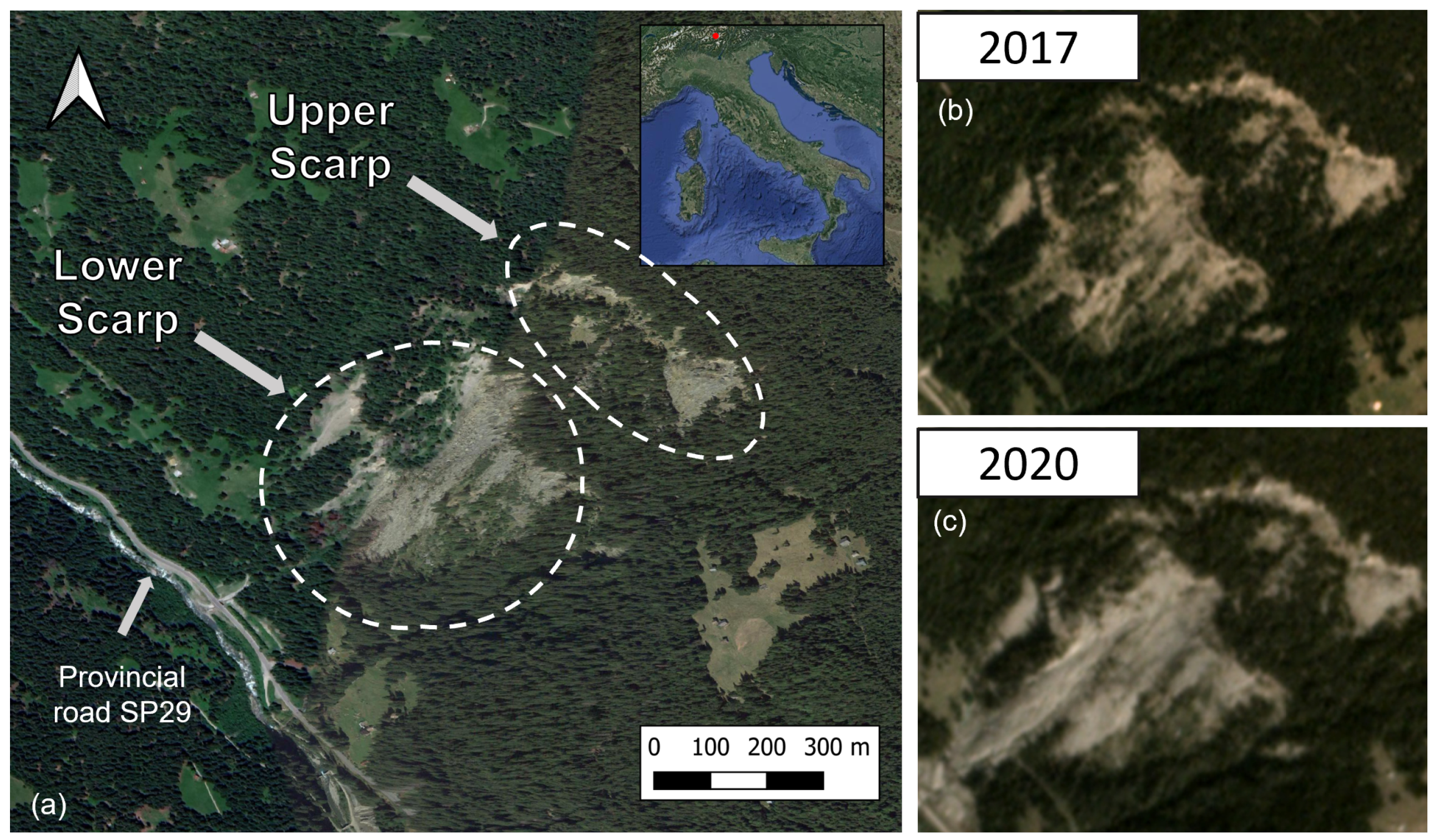
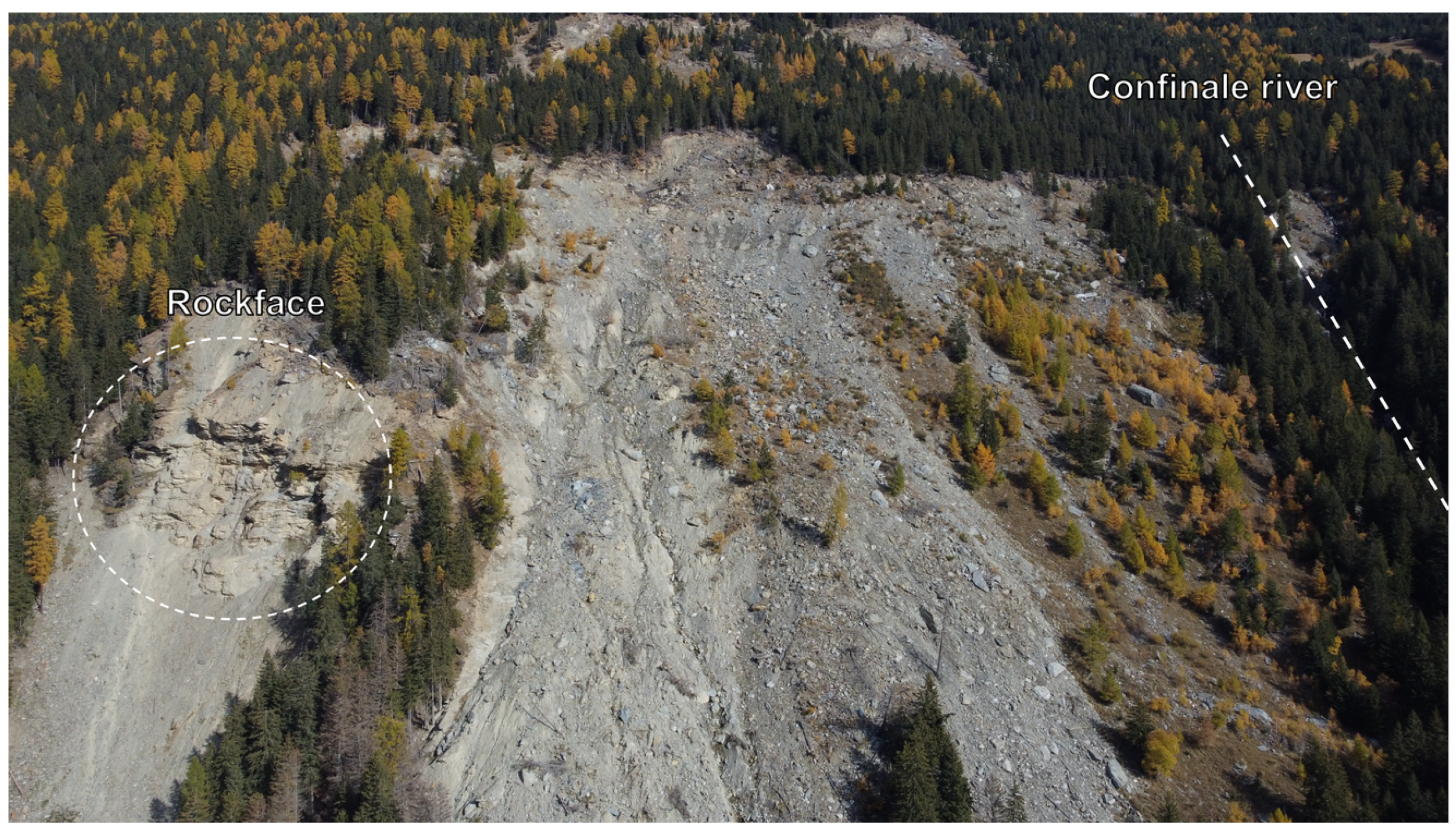
2.1. Case Study—Ruinon Landslide

The Ruinon landslide (Figure 1) is located in the Upper Valtellina, Northern Italy, and is one of the most active rockslides in the Italian Alps. Throughout the years it has been under continuous investigation and monitoring from scholars, experts and local authorities [31,32,33]. The active Ruinon landslide actually lies on top of a deep-seated gravitational slope deformation (DSGSD), recognized in 1998 [34], while local failures were documented from 1954, with several airborne surveys of the area having been organized as early as 1954 and 1981 by the Lombardy regional authorities [31].
While the DSGSD reaches up to 3000 m a.s.l almost on the whole hillslope, the Ruinon landslide is divided into two scarps, the lower ranging from around 1400 to 1900 m a.s.l, and the upper at around 2100 m a.s.l. In the last few years, the more active scarp has been the lower one, with planar and toppling failures which has resulted in displaced debris of various sizes (from gravel size to about 10 m). The main body of the lower scarp is bounded on the left-flank side by the Confinale river and on the right by an almost vertical rockface, and currently, the toe reaches a newly constructed rock barrier for protecting Provincial Road SP29 (Figure 2).
In fact, SP29 is the main connection to Santa Caterina di Valfurva, a small village home to famous ski resorts. Throughout the years, reactivations at Ruinon were a direct threat to people’s lives, but also to the socioeconomic state of the region. The occurrence of failures has a recurrent character, with activations predominantly occurring during the summer–autumn months, with relatively calmer periods over the winter period. Such recurrent activities have already been monitored and reported almost every year since 2006, when a permanent Ground-Based Interferometric Synthetic Aperture Radar (GBInSAR) system was installed [32,34,35,36]. Aside from the GBInSAR, the landslide has been monitored since 1997 through a manual and automatic geotechnical network [33]. In addition to the data from permanent ground stations during the last two decades, the Ruinon landslide was also monitored through spaceborne optical and radar missions [36,37], which recorded the most disastrous reactivations during the summers of 2016, 2018 and 2019. During the year 2021, no significant critical activities on the landslide body were reported [38].

2.2. Workflow

Excluding the actual UAV surveys, the implemented workflow in this work is generally divided into four main steps (Figure 3): processing the acquired datasets; post-processing their products; producing Red Relief Image Maps and applying a finer co-registration, and final displacement computation. To carry out a time-series analysis using the UAV-derived products, we used two separate datasets: six surveys carried out during the period 2019–2020 by the Regional Agency for the Protection of the Environment (ARPA) of the Lombardy Region (Section 2.3.1), and surveys carried out by us in the period 2021–2022 (Section 2.3.2). Both datasets will be further presented in the relevant sections. As there were generic differences between the datasets, the 2019–2020 set being composed only of point clouds and orthophotos, a post-processing step was needed to put them in a common framework, for example, with spatial subsampling of the point clouds, co-registration, etc. This step was followed by producing the RRIM for each epoch and a step-wise finer co-registration of the maps carried out into two sub-steps—a local co-registration of the stable regions and a global one for the unstable parts. The last step was the computation of the dense optical flow and vector magnitude. To ensure higher reproducibility, all the steps were carried out using only Free and Open Software Solutions (FOSS) and Python packages. Namely, for producing the point clouds, DSM and orthoimages were processed with OpenDroneMap [39], CloudCompare [40] was used for their co-registration, Relief Visualization Toolbox for Python [41] for producing RRIMs, and the Lucas–Kanade implementation in the scikit-image Python package [42] for displacement computation.

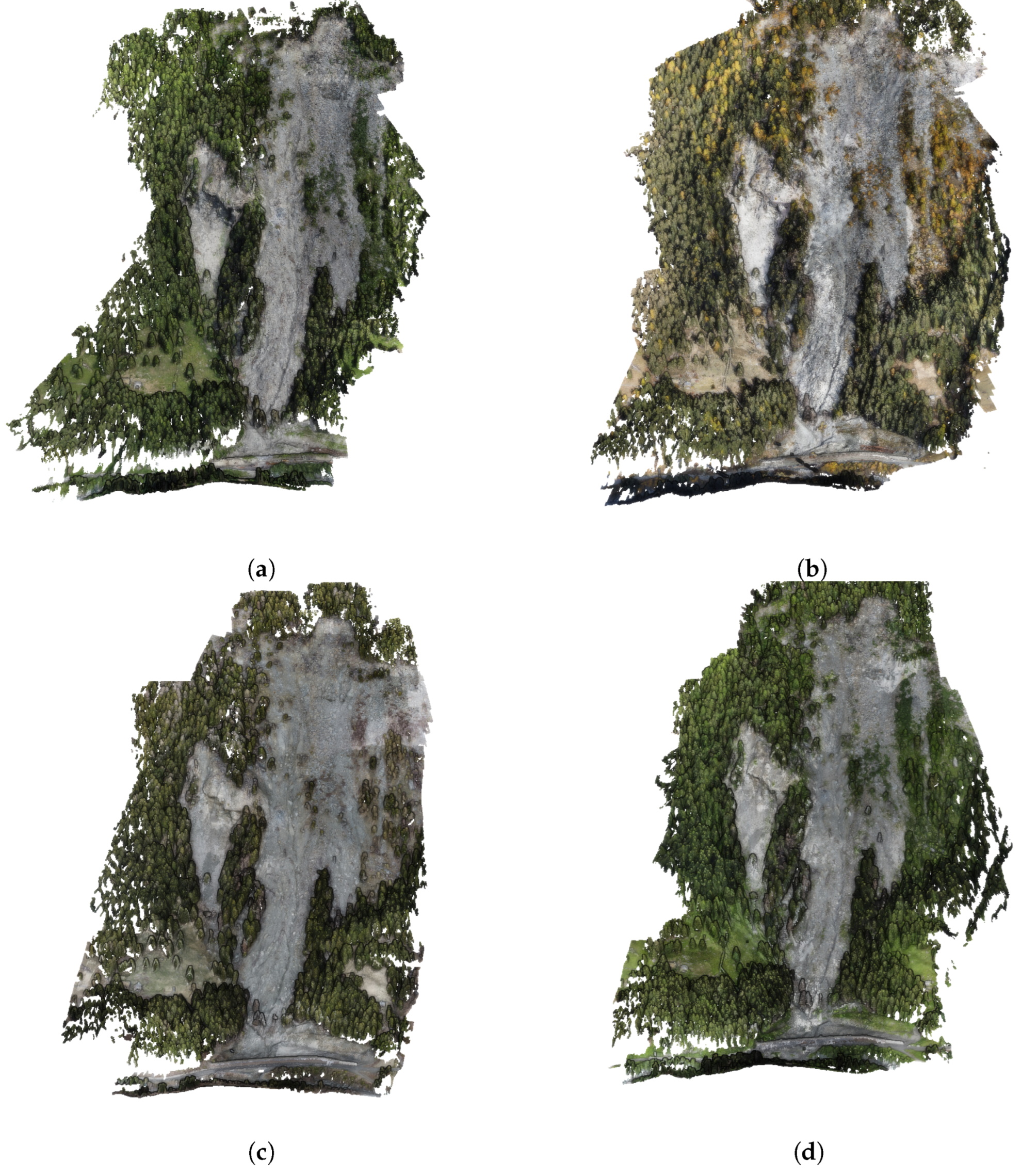
2.3. UAV Surveys and Their Outcomes

2.3.1. Period 2019–2020

In addition to the permanent monitoring station, during the period of 2019–2020, and due to continuous Ruinon activations, the local agency ARPA carried out UAV surveys over the area. Upon request, the resulting point clouds and orthophotos were shared with us. In Table 1, the dates of acquisition, as well as the reconstructed points are reported, while the point clouds are shown in Figure 4. As we were provided only with the output products, there is no information related to the survey or flight parameters, nor captured images per survey. Moreover, during the data acquisition or surface reconstruction steps for those specific surveys, Ground Control Points (GCPs) were not used, and therefore they could not be evaluated in terms of accuracy. In addition, by visual inspection, significant local and global misalignments among the different epochs were noted. A different amount of reconstructed points was also noticeable, where the first products were sparser compared to the latest. However, the aforementioned issues were overcome with post-processing (Section 2.4), and the point clouds were sufficient as initial input to be incorporated into the analysis.

2.3.2. Period 2021–2022

As part of our surveys, four flyovers were carried out during the period 2021–2022, over the same Ruinon landslide area. The main idea was the continuation of the surveys in terms of time and adopting novel approaches for monitoring landslide phenomena. Moreover, carrying out the surveys first-hand provides full control over all activities from the planning stage to the final outputs. As the recent reactivations were during summer periods, the surveys were planned to be before and after potentially unstable periods, i.e., spring and autumn periods were most suitable. The current work follows and extends the scope of a previous one [43] in which the main principles of UAV survey planning and processing were explained in detail, to be easily adoptable and reusable in other research domains (e.g., archaeology and glaciology [44,45]). A brief summary of the setup and steps will be presented below.
All of the surveys were made using a consumer-grade quadrotor DJI Mini 2 (249 gr.) equipped with a built-in position system able to connect to GPS, GLONNAS and GALILEO constellations. The UAV has a 12 MP CMOS sensor with an f/2.8 lens onboard. Some of the advantages of using this aircraft can be related to its size and weight. The low body weight puts the model into a low-risk category for which, according to the European regulations [46], the operator needs to do a short online course and exam. The small aircraft has wind resistance at level 5, an advantage considering the weather conditions which may occur during a landslide survey in mountainous areas. On the other hand, there are some drawbacks of the UAV, again related to body size and weight. For instance, the quadrotor lacks an obstacle avoidance system, from through which other optional features such as designing and following a survey plan are also missing. To overcome the lack of mission planning, Flight Planner [47] was used, which is a QGIS [48] plugin useful for planning airborne photogrammetric surveys. The plugin needs three main inputs—vector shape of the area of interest, digital elevation model (DEM), and target ground sampling distance (GSD), with the outputs being projection centers, flight paths and waypoints.
After data acquisition, the collected images were used to produce point clouds, digital surface models and orthophotos, using the OpenDroneMap tool [39], which is a FOSS for processing aerial data based on state-of-the-art Structure from Motion (SfM) and Multi-View Stereo (MVS) approaches. A summary of the point cloud characteristics is reported in Table 2 and visualized in Figure 5.
During the surveys, at least five GCPs were placed and measured using Leica AX1200 in real-time kinematic positioning (RTK) mode connected to Bormio permanent reference station (https://www.spingnss.it/, accessed on 28 October 2022). Three independent measurements were made for each marker. The GCPs were distributed in an area considered stable and far from landslide movements (see Figure 4 in [43]). It should be noted that the GCPs used are not distributed in optimal positions around the landslide body, but, considering its size, terrain and the fact that it is still an active area, field activities at higher altitudes towards the crown were not allowed.
The final products achieved the targeted GSD and all of the outputs have a spatial resolution of at least 10 cm/pix or better. All orthophotos are available and free for download from the platform for sharing aerial images OpenAerialMap (accessed on 30 October 2022) https://map.openaerialmap.org/#/10.358734130859375,46.45630839492814,10/square/120221312?_k=hzzlob. It should be noted that all surveys followed the same case-specific flight plan and processing scheme. Namely, maximum flight altitude was always 110 m above ground; when flying in a longitudinal direction 11 tracks with vertical speed maintained at 3 m/s were followed, horizontal speed at 4.5 m/s; camera inclination was at −57 , while in transversal directions; 14 paths were flown with the vertical speed at zero and horizontal at 6 m/s; the camera was set at −90 . However, as mentioned before, the UAV lacks autonomous flight, therefore all were carried out manually by an operator, maintaining the above-mentioned parameters, which can explain the small differences in the reconstructed points. Among all of them, the one with the sparsest point cloud is that of the 5 July 2022 survey. Even after a deep investigation, the reason for this lower point density could not be determined, as the detected and reconstructed features were very similar in location and count compared to the rest of the products. Nevertheless, the output was still suitable for the following processing steps.
At a first glance, it can be noted that all of the point clouds cover the whole landslide body (including 2019–2020) and the main changes on its surface are visible. However, it can also be noted that point clouds are produced under different light conditions and vegetation states. This problem will create challenges and errors when applying surface displacement analysis, an issue which we are trying to solve with the current work.

2.4. Postprocessing

The survey outputs are from different sources and used different processing techniques which, naturally, leads them to exhibit diverse characteristics and the need to be placed in a common framework, mainly to produce coherent DSMs for the 2019–2021 period. These steps were performed mostly using CloudCompare [40] with only final filtering applied in QGIS, including:
  • Spatial sampling of the point clouds to achieve relatively similar density (set to a minimum distance of 10 cm).
  • Co-registration of the point clouds: In most cases, Iterative Closest Point (ICP) co-registration was sufficient; when it was not, it was also performed manually using common points between the clouds. The 2019–2020 dataset had unknown accuracy, and it was decided that those epochs should be co-registered according to 2021–2022, specifically, the 6 July 2021 survey was set as a reference point. However, the changes during the 2019–2020 period were severe ,and therefore the moving primary scheme was applied in reverse order, i.e., 19 October 2020 was co-registered to 6 July 2021, 25 October 2019 to 19 October 2020, etc. On the other hand, the epochs in the 2021–2022 period were co-registered using a fixed primary scheme and all three products were transformed according to 6 July 2021. The achieved co-registration error varied among the epochs in the range of 0.20 m < RMS < 0.30 m, and most of the highest values were in the 2019–2021 dataset.
  • The co-registered point clouds were rasterized into DSM with a spatial resolution of 10 cm/pix.
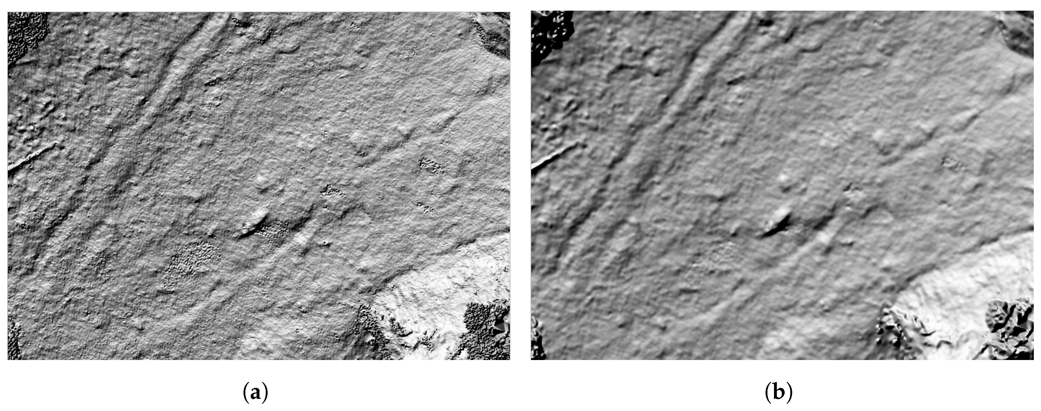
  • Filtering the resulting DSMs: As the point density was reduced to a certain level, the interpolation of the point cloud into raster led, in some cases, to noisy and irregular terrain, which may further alter the analysis. A Gaussian filter (kernel type—square and radius of 3 pixels) was applied to obtain a more regular and smooth surface product without losing details (e.g., Figure 6).

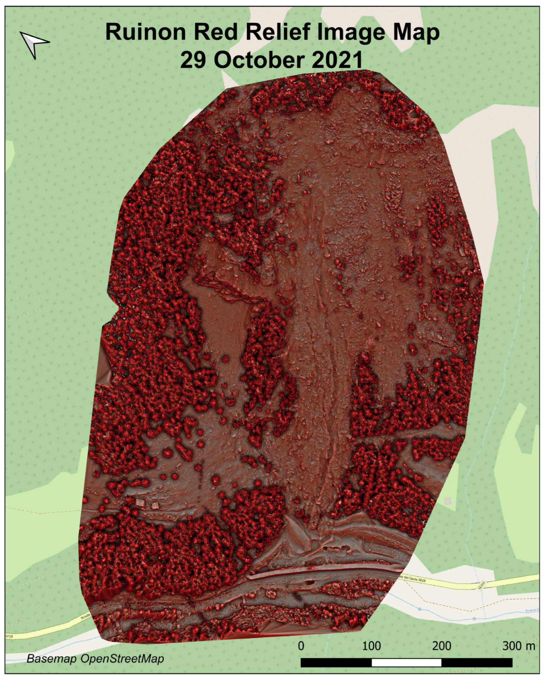
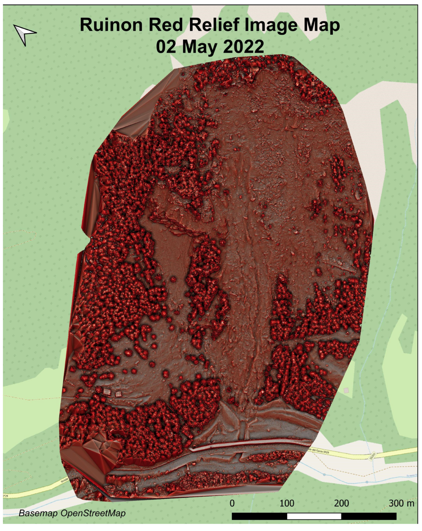
2.5. Red Relief Image Map

Red Relief Image Map (RRIM) is a visualization technique introduced by Chiba et al. [27] as a method for highlighting topographic features in greater detail. The implementation of RRIM is an extension of the parameter openness [28], introduced as an image-processing technique which emphasizes the concavities and convexities of the surface, combined with the slope gradient. The RRIM technique is proposed as an alternative visualization approach to topographic information, based on the better perception of the color red by the human eye. In particular, the method relies on differential openness:
O p O n 2 ,
where O p is the positive openness, i.e., the convexity of a surface, and O n is the negative openness, i.e., the concave features of a surface. Once computed, the differential openness is blended with a slope gradient layer which is pseudo-colored in red. An example is shown in Figure 7, depicting the area of Upper Valtellina as separate products needed to produce RRIM using SRTM30 data, including also a satellite view and a hillshade visualization.
Black color RRIM depicts concave features, and white convex and grey colours are flat surfaces. In the red gamut, steep slopes are highlighted with a saturated red colour, with convexity and concavity in the lower range. An important parameter for the computation of both positive and negative openness is the radial limit (i.e., the search radius of the moving window), which is directly linked to the level of detail to be highlighted.
Looking at the figure, the advantages of using the RRIM visualization are evident. On the one hand, it enhances the perception of detail and depth, compared to the optical image or the hillshade visualization, on the other hand, it is not altered by the sunlight direction, shadows, and vegetation state. Those particular features are of great benefit when applying algorithms for computer vision, especially for a landslide monitoring task. The RRIM clearly depicts topographic features of various sizes and shapes, even on flat surfaces, and even if the level of the details is obviously highly dependent on the resolution and quality of the input dataset.
The tool used for producing RRIM was the Relief Visualization Toolbox for Python [41,49]. It is a set of instruments aiming to generate various visualizations of elevation models with a focus on small-scale features. Some of the implemented methods include but are not limited to, multiple-direction hillshading, a simple local relief model, sky-view factor, etc. RRIM is not directly available off the shelf but the Relief Visualization Toolbox can be easily adjusted for that purpose.

2.6. Dense Optical Flow

In this work, a traditional dense optical flow technique for determining the apparent motion of features in the image space [50] between two consecutive instances was used. In the last couple of decades these techniques have been widely used in computer vision problems [51,52], as well in the domain of Earth Observation [20,53,54]. For the current implementation, we took advantage of the Le Besnreais and Champagnat [55] implementation of the Lucas–Kanade [26] dense optical flow using iterative registration, which works with a ’local’ search window approach for brightness pattern shifts. It is very cost-efficient due to the coarse-to-fine inverse pyramid strategy for the window search. Since it is a method based on image intensity, a few drawbacks can occur during its implementation: an abrupt change in illumination between two images can create shadows which influence pixel brightness; vegetation state can also change between two surveys. In addition to intensity-related issues, it is important to have the products properly co-registered because local or global shifts would be also considered as motion. Such problems will lead to de-correlated and wrongly oriented vector fields in the final product.
In this work, the Iterative Lucas–Kanade approach was used through its implementation in the scikit-image Python package [42]. As it was also used for image registration, we implemented the dense optical flow computation in two steps: (1) finer image co-registration (Section 2.6.1) and (2) the actual landslide displacement computation (Section 2.6.2).

2.6.1. Finer Co-Registration

Since the phenomenon we are trying to model is dynamic, a direct image-to-image registration cannot be applied, as some of the areas can be wrongly wrapped to their initial position, even though it is an actual displacement. To overcome the issue and to obtain a finer co-registration of two consecutive products, a dense optical flow approach was applied at two instances for the secondary image (Figure 8). Firstly, a local co-registration was performed on stable parts outside the active deformation, followed by more rigid shift correction which does not interfere with the actual debris displacements, and finally, both co-registered segments are combined in one. Note that high and consistent shift values may be an indication of decorrelation due to insufficient overlap between two images.

2.6.2. Displacement Computation

The final step of processing is the actual displacement computation. The merged co-registered secondary image from the previous step was used directly to compute the displacements compared to a previous epoch. The output of the processing gives the displacement vectors in the u,v directions, from which the magnitude of the displacement can be easily computed:
| | u , v | | = u 2 + v 2 ,
and the orientation of the vector
θ = t a n 1 ( v u ) .
Since the UAV was manually operated during the surveys, some ambiguities in the reconstruction part can be seen. This is evident in the reconstruction of vegetation (bushes and trees). Due to this drawback, after the displacement magnitude and orientation computation, many decorrelations can be depicted. They are most notable when inspecting the vector orientations, depicting movements parallel to the general slope or even upslope. To mitigate this issue and keep only the relevant displacement, a filter according to the displacement orientation was applied. The general slope orientation of the landslide was estimated to be at 225 (North is at 0 ). The applied filter took into account this dip direction ± 45 , and therefore the kept displacements were only the ones orientated between 180 and 270 . The ± 45 range deviation from the actual dip direction was chosen due to the current work scale and the fact that the movement trajectory of some small debris does not need to exactly follow direct downslope shifts, since they can easily deviate from it.

3. Results

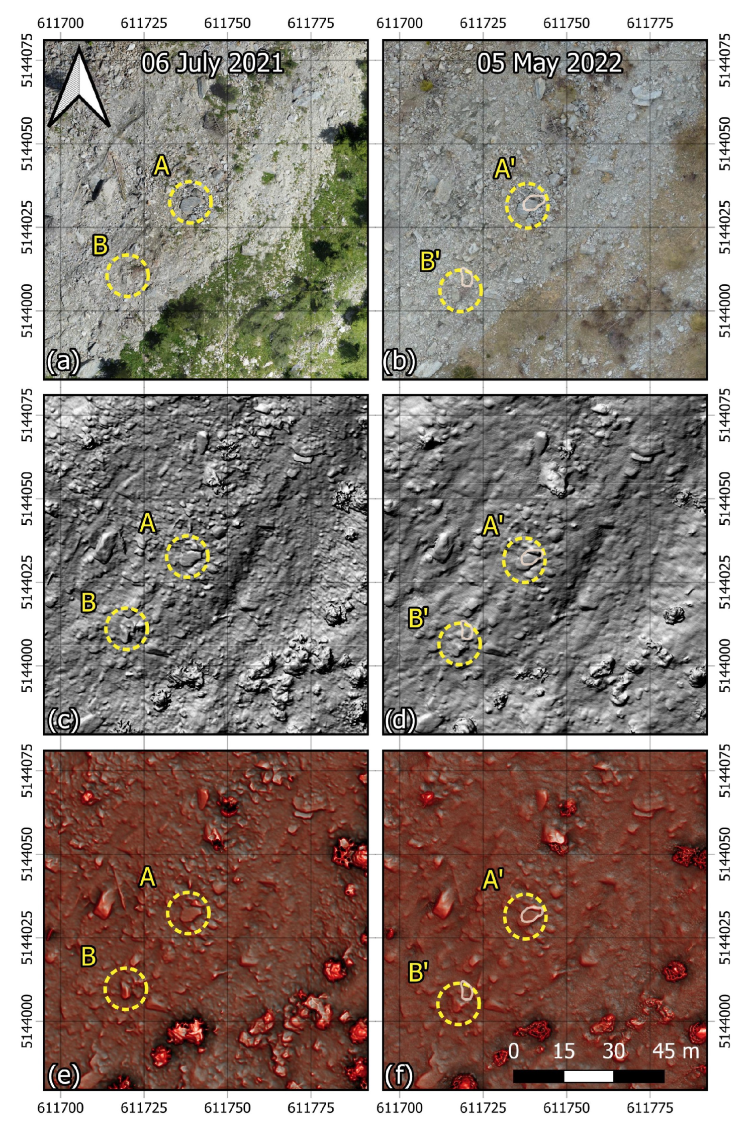
3.1. RRIM Implementation

Following the previously discussed processing workflow scheme, ten red relief image maps for the period 2019–2022 were obtained as outputs from the UAV surveys of the Ruinon landslide with a non-regular time-series. The advantages of using RRIMs compared to orthophotos for applying computer vision approaches are better highlighted at lower scale representation. To show this fact, details of the RRIM implementation in comparison to orthophotos and hillshade visualization are depicted in Figure 9, while the full-scale RRIMs for the period 2021–2022 are added as an Appendix A.1, Appendix A.2, Appendix A.3 and Appendix A.4 (available [56]).
For a full comparison with the orthophotos, the latter can be accessed as mentioned in Section 2.3.2 from the https://openaerialmap.org/ (OpenAerialMap.org, accessed on 30 October 2022) platform. The two rows of image subsets (Figure 9) depict the same subregions of the landslide body during two different periods—summer (6 July 2021) and spring (5 May 2022). Clear differences are notable in the orthophotos (Figure 9a,b), mainly associated with the lighting conditions and vegetation state. In the first example strong shadows are present which are increase the visual depth perception of the image, but so are defining areas with high contrast and a lack of detail in the underexposed areas. On the other hand, the second instance was a result of a survey carried out during an overcast day lacking direct sunlight, which created a consistent illumination of the terrain without harsh shadows but also lacks clear contrast among the objects. Examples of the different conditions are the two highlighted boulders A and B with their related displaced locations (A’,B’). Moreover, there is a strong difference in the vegetation state growing on the landslide body with seasonal variation—in July the leafage is at its maximum, while in May there are still signs of wilted grass and shrubs. From the perspective of determining displacements through intensity-based computer vision approaches, these factors are critical as they may greatly worsen the final results. As a solution, implementing RRIM can significantly aid in visualizing a normalized representation of the terrain and provide a better map on which to apply intensity-based algorithms.

3.2. Displacement Computation

In the following section, the results of the application of dense optical flow for displacement computation between two consecutive survey epochs, i.e., using the so-called moving primary strategy, are presented. The approach was applied to the RRIMs which were also finely co-registered by two independent iterations—one reducing local shifts over the stable areas outside the unstable slope, followed by another more rigid (global) co-registration of the actual landslide body. As highlighted by the results (Figure 10), the landslide was mostly active in the period 26 July 2019 to 6 July 2021, while the exact initial and final dates cannot be determined due to a lack of observations.
It is important to mention the fact that the reported displacements are already filtered according to the moving direction and refer only to two-dimensional XY displacements. Moreover, the visualized arrows depict only the movement direction, and their length is not associated with the magnitude of the displacement. Upon inspection of the maps in Figure 10, the most distinguishable movement can be seen to be amid the central landslide body and, especially during the initial four periods, the most active and severe parts are at the upper and central areas.
Interestingly, there is the appearance of a zero-displacement patch of the magnitude field starting from the first period (Figure 10a) and “moving” downhill at each following epoch (Figure 10b–d). Upon visual interpretation of the RGB orthomaps, it was determined that those areas, at the initial stages, were forested and then shattered by displaced debris at different stages of the mass movement. In contrast, the actual reason for them to appear “stable” with zero displacements was actually the decorrelation between two consecutive RRIMs in those specific regions, i.e., the abrupt landcover change from forest to debris made it impossible for the algorithm to find corresponding pixels and works only in 2D space without accounting for changes along the elevation axis. Similar decorrelation zones can be also noted in the sequential periods. After 14 September 2019, there is a significant, yet gradual, intensity decrease of the estimated surface displacements, whereas after 6 July 2021, some sporadic movements were mapped which upon visual validation are either from single displaced boulders or inconsistent reconstructions of shrubs and trees. Such false positive displacements, due to the presence of vegetation, are not rare, however, in these cases, the “detected” displacements are isolated and do not exhibit a spatio-temporal coherence among the epochs.
On the other hand, an example of a localized movement with a spatial consistency over time can be easily recognized on the left landslide flank (Figure 10e–g), exhibiting a triangular shape active during the main body reactivations. However, during the period between 6 July 2021 and 29 October 2021, this was the only main debris displacement mapped, and it was not further detected during the following observations.
The overall displacement magnitude can be inspected by epoch using box plots (Figure 11), highlighting the general decrease in the trend of surface displacements and re-occurring major reactivation during the fourth period (25 October 2019–10 September 2020), best seen in the median value (vertical line in the boxes). From the available observations, only a couple of epochs exhibit magnitudes higher than 10 m, namely the first and fourth, which does not mean that the rest are of negligible intensity. The summary box plots of magnitude (Figure 11) is further evidence of the false-positive displacements marked as outliers (denoted as dots) from the overall magnitude field of the epoch.

4. Discussion

The current work proposed an approach for obtaining landslide displacements using time-series-derived UAV datasets. The primary research problem that needed to be solved was related to inherited discrepancies in the datasets themselves. Some common ground characteristics were present among them, such as that the surveys were carried out over the same area of interest and the same type of sensor was used, namely, an optical RGB sensor. This is the extent of the commonalities and different features such as camera sensor model, airborne platform, the experience of the UAV operator, post-processing techniques, illumination conditions and vegetation state prevailed. Thus, present datasets over time can provoke difficulties in their usage, especially when the approach to be adopted, such as dense optical flow, is sensitive to image intensity [20,25]. To overcome such issues, the adoption of RRIM [27], a visualization technique directly applied to DSM products of the UAV surveys, was proposed. With the use of normalized images, the use of the resulting maps was instrumental in overcoming an issue related to different and unfavorable illumination conditions that could alter the application of dense optical flow directly on orthoimages.
The combination of different approaches resulted in a successful method for detecting movements at various scales, from highly intensive periods where the central part of the landslide collapsed, as a whole (e.g., Figure 10a–f and Figure 11), to some smaller localized instabilities such as the aforementioned zone on the right landslide flank (best visible at Figure 10g).
In fact, the latter would have been difficult to distinguish through more conventional approaches, such as point cloud comparison using a Multiscale Model to Model Cloud Comparison (M3C2) [57] approach or cross-sections [58]. As depicted in Figure 12, our approach accurately estimates the spatial extent and magnitude field for the localized movement which is not really clearly highlighted within the same intensity range in the M3C2 comparison of the point clouds (Figure 12b) for the same period. On the other hand, using DSMs it is also possible to manually inspect the elevation profiles from both surveys at a smaller scale (Figure 12c) and to compare the measurements for a particular location. The represented elevation profile actually is a fraction of the central landslide body (>500 m), and using cross-sectional elevation profiles could make the detection of such localized movement almost impossible.
By changing the spatial and intensity scale, the approach succeeded in precisely estimating velocity vectors through the epochs of the most severe reactivations of the central part of the landslide body, which obviously cannot be considered for estimating volumetric changes and more abrupt land cover changes (e.g., loss of forested areas). Some of our results derived from the 2019 surveys (Figure 10a–c) are consistent with the results obtained from another approach we implemented for estimating Ruinon reactivations through Sentinel-2 imagery [37]. Furthermore, comparable outputs for the Ruinon landslide are reported by Carla et al. [36], with the difference that their work utilized a GBInSAR monitoring technique. In the aforementioned work, some of the observations for 2019 are reported per month, in the current work, in contrast, we do not have surveys that cover exactly a full month and could be used for comparison. However, the intensity of our initial 3 epochs from 2019 is similar to their monthly cumulative displacements from August to October 2019. Moreover, the estimated extreme displacements from the GBInSAR coincide with our patches with lost coherence (already discussed in Section 3.2). Similarly, if we produce a cumulative map for the period 4 September 2019 to 25 October 2019 (Figure 13), our patch of no coherence is at a location that coincides with a zone with displacements higher than 50 m for the same period (in [36]). Moreover, the areas directly around the patch of no coherence exhibit comparable magnitude fields.
It needs to be highlighted that the optical flow computation, i.e., in this case the displacement computation, is sensitive to the search radius parameter. By applying a low value, the algorithm cannot find the corresponding location outside a certain range. Therefore, such cases as the ones mentioned before can occur, and the relevant result can exhibit zero displacement, even if this is not true. The issue can be overcome by simply increasing the radius, but this has to be done without overestimating since this approach can lead to the opposite effect—falsely “detecting” certain features or exaggerating their magnitudes. Therefore, this parameter’s value is highly dependent on the case study under investigation.
A possible limitation of the proposed approach is related to the already mentioned fact that it can only estimate displacements in the 2D-space plane, disregarding movements along the vertical axis, and further implementation of similar approaches for 3D motion estimation either on point clouds or voxels is the natural continuation of the current work. Similarly, the approach estimates displacements in the 2D-space, but an essential part of it is a DSM to derive an RRIM. Without elevation data, the topographic visualization could not be applied to obtain a normalized image map. Still, the displacement estimation could be applied directly on an orthomap, yet the results should be considered with great attention as many errors could occur if orthomaps have inherently different image intensities (i.e., great variations in brightness and contrast). Further improvements could also be related to an application of spatial consistency filters which can disregard inherited errors from the reconstruction process, similar to the previously discussed issues with vegetation. It is worth pointing out that this is not a very straightforward task as there is always the possibility that such a filter can ignore movements that are not spatially or temporally coherent for the particular time series.
The presented methodology successfully delivered more than satisfactory results, as it was set to solve challenging problems related to, on the one hand, the utilization of input field surveys from different sources, and on the other, the analysis of a significant landslide which exhibits reactivations that are non-coherent in terms of space, time and intensity. Due to the higher spatial resolution outputs from this approach, it can be further utilized for validation purposes regarding other methodologies that use lower-resolution datasets, such as satellite-derived ones. Overall, the setup can be considered low-cost and computationally inexpensive, allowing deployment for regions and mass movements where no permanent monitoring stations and tools are available, with further tuning of the time intervals according to specific needs.

5. Conclusions

The Ruinon landslide is a landslide that has been documented for more than two decades and which has occasionally reactivated, as in the last years. As such, it has served as an interesting case study for scholars to perform various investigations, whether they are field-based or remote (close-range or air-/space-borne), which further provides invaluable input and output for further developing and testing new approaches. The current work presents a method combining a low-cost UAV surveying setup with a topographic visualization technique, RRIM, and a computer-vision-based algorithm for movement estimation. The utilized consumer-grade quadrotor proved to be convenient from a regulation point of view and in delivering high-resolution images, which were further used for scene reconstruction in the form of point clouds, DSMs and orthorectified maps. Along with our own surveys, the time series dataset was further extended with other datasets provided to us. Combining data products from different sources entailed a normalization step to be included in processing. For this reason, the Red Relief Image Mapping technique was applied to the elevation models, which had a two-fold effect. On the one hand, the datasets from different sources were put into a common framework, and on the other hand, it solved the issue of different unfavorable illumination conditions during the surveys. The latter is in fact a significant issue when an intensity-sensitive algorithm for motion estimation, in this case—the Lucas–Kanade optical flow, is applied. With the results from the method we have presented in this paper, we successfully derived surface mass movements within different spatial and intensity scales, from a few centimeters to more than several tens of meters. Moreover, the resulting accurate outputs are produced in a computationally efficient manner through the use of free and open-source software which further allows for the method’s straightforward adaptation and modification in other case studies. Several follow-up research directions could potentially further contribute to the approach, namely, a transition from 2D space to 3D and an application of a filter for spatial coherency, helping to disregard false estimations. Nevertheless, even in this simplified version, our approach can at least contribute to the validation of remotely sensed lower-resolution products and to the monitoring of landslides that are not permanently monitored in situ.

Author Contributions

Conceptualization, V.Y. and M.A.B.; methodology, V.Y.; software, V.Y.; validation, V.Y. and Q.X.T.; writing—V.Y.; writing—review and editing, V.Y., M.A.B. and Q.X.T.; supervision, M.A.B. and Q.X.T.; funding acquisition, M.A.B. All authors have read and agreed to the published version of the manuscript.

Funding

This work is partially funded by the Italian Ministry of Foreign Affairs and International Cooperation within the project “Geoinformatics and Earth Observation for Landslide Monitoring”—CUP D19C21000480001 (Italian side) and partially funded by the Ministry of Science and Technology of Vietnam (MOST) (Vietnamese side) by the Bilateral Scientific Research project between Vietnam and Italy, code: NĐT/IT/21/14.

Data Availability Statement

Data available upon request.

Acknowledgments

Acknowledgments to everyone contributing to the project, to Ludovico Biagi and Marianna Alghisi from Politecnico di Milano for the GNSS surveys, to ARPA Lombardia for providing us with the datasets and to Parco Stelvio for authorizing the UAV surveys.

Conflicts of Interest

The authors declare no conflict of interest. The funders had no role in the design of the study; in the collection, analyses, or interpretation of data; in the writing of the manuscript; or in the decision to publish the results.

Abbreviations

The following abbreviations are used in this manuscript:
DSGSDDeep-seated gravitational slope deformation
GBInSARGround-Based Interferometric Synthetic Aperture Radar
ARPARegional Agency for the Protection of the Environment (from Italian)
RRIMRed Relief Image Map
UAVUnmanned Aerial Vehicle
FOSSFree and Open Software Solutions
GCPsGround Control Points
CMOSComplementary Metal-Oxide-Semiconductor
SfMStructure from Motion
MVSMulti-View Stereo
RTKReal-Time Kinematic
DSMDigital Surface Model
ICPIterative Closest Point
M3C2Multiscale Model to Model Cloud Comparison
m. a.s.l.Meters above sea level

Appendix A

Appendix A.1

Figure A1. Ruinon Red Relief Image Map 6 July 2021.
Drones 07 00085 g0a1

Appendix A.2

Figure A2. Ruinon Red Relief Image Map 29 October 2021.
Drones 07 00085 g0a2

Appendix A.3

Figure A3. Ruinon Red Relief Image Map 2 May 2022.
Drones 07 00085 g0a3

Appendix A.4

Figure A4. Ruinon Red Relief Image Map 5 July 2022.
Drones 07 00085 g0a4

References

  1. Scaioni, M.; Longoni, L.; Melillo, V.; Papini, M. Remote sensing for landslide investigations: An overview of recent achievements and perspectives. Remote Sens. 2014, 6, 9600–9652. [Google Scholar] [CrossRef] [Green Version]
  2. Pradhan, B.; Lee, S.; Mansor, S.; Buchroithner, M.; Jamaluddin, N.; Khujaimah, Z. Utilization of optical remote sensing data and geographic information system tools for regional landslide hazard analysis by using binomial logistic regression model. J. Appl. Remote Sens. 2008, 2, 023542. [Google Scholar] [CrossRef]
  3. Hervás, J.; Barredo, J.I.; Rosin, P.L.; Pasuto, A.; Mantovani, F.; Silvano, S. Monitoring landslides from optical remotely sensed imagery: The case history of Tessina landslide, Italy. Geomorphology 2003, 54, 63–75. [Google Scholar] [CrossRef]
  4. Schönfeldt, E.; Winocur, D.; Pánek, T.; Korup, O. Deep learning reveals one of Earth’s largest landslide terrain in Patagonia. Earth Planet. Sci. Lett. 2022, 593, 117642. [Google Scholar] [CrossRef]
  5. Mondini, A.C.; Guzzetti, F.; Chang, K.T.; Monserrat, O.; Martha, T.R.; Manconi, A. Landslide failures detection and mapping using Synthetic Aperture Radar: Past, present and future. Earth-Sci. Rev. 2021, 216, 103574. [Google Scholar] [CrossRef]
  6. Burrows, K.; Marc, O.; Remy, D. Using Sentinel-1 radar amplitude time series to constrain the timings of individual landslides: A step towards understanding the controls on monsoon-triggered landsliding. Nat. Hazards Earth Syst. Sci. 2022, 22, 2637–2653. [Google Scholar] [CrossRef]
  7. Yordanov, V.; Biagi, L.; Truong, X.Q.; Tran, V.A.; Brovelli, M.A. An Overview of Geoinformatics State-of-the-Art Techniques for Landslide. Int. Arch. Photogramm. Remote Sens. Spat. Inf. Sci. 2021, 46, 205–212. [Google Scholar] [CrossRef]
  8. Handwerger, A.L.; Jones, S.Y.; Huang, M.H.; Amatya, P.; Kerner, H.R.; Kirschbaum, D.B. Rapid landslide identification using synthetic aperture radar amplitude change detection on the Google Earth Engine. Nat. Hazards Earth Syst. Sci. Discuss. 2020, 2020, 1–24. [Google Scholar] [CrossRef]
  9. Aslan, G.; Foumelis, M.; Raucoules, D.; De Michele, M.; Bernardie, S.; Cakir, Z. Landslide Mapping and Monitoring Using Persistent Scatterer Interferometry PSI Technique in the French Alps. Remote Sens. 2020, 12, 1305. [Google Scholar] [CrossRef] [Green Version]
  10. Giordan, D.; Hayakawa, Y.; Nex, F.; Remondino, F.; Tarolli, P. Review article: The use of remotely piloted aircraft systems (RPASs) for natural hazards monitoring and management. Nat. Hazards Earth Syst. Sci. 2018, 18, 1079–1096. [Google Scholar] [CrossRef] [Green Version]
  11. Valkaniotis, S.; Papathanassiou, G.; Ganas, A. Mapping an earthquake-induced landslide based on UAV imagery; case study of the 2015 Okeanos landslide, Lefkada, Greece. Eng. Geol. 2018, 245, 141–152. [Google Scholar] [CrossRef]
  12. Kotsi, E.; Vassilakis, E.; Diakakis, M.; Mavroulis, S.; Konsolaki, A.; Filis, C.; Lozios, S.; Lekkas, E. Using UAS-Aided Photogrammetry to Monitor and Quantify the Geomorphic Effects of Extreme Weather Events in Tectonically Active Mass Waste-Prone Areas: The Case of Medicane Ianos. Appl. Sci. 2023, 13, 812. [Google Scholar] [CrossRef]
  13. Sestras, P.; Bilasco, S.; Rosca, S.; Dudic, B.; Hysa, A.; Spalevic, V. Geodetic and UAV Monitoring in the Sustainable Management of Shallow Landslides and Erosion of a Susceptible Urban Environment. Remote Sens. 2021, 13, 385. [Google Scholar] [CrossRef]
  14. Godone, D.; Allasia, P.; Borrelli, L.; Gullà, G. UAV and Structure from Motion Approach to Monitor the Maierato Landslide Evolution. Remote Sens. 2020, 12, 1039. [Google Scholar] [CrossRef] [Green Version]
  15. Casagli, N.; Frodella, W.; Morelli, S.; Tofani, V.; Ciampalini, A.; Intrieri, E.; Raspini, F.; Rossi, G.; Tanteri, L.; Lu, P. Spaceborne, UAV and ground-based remote sensing techniques for landslide mapping, monitoring and early warning. Geoenviron. Disasters 2017, 4, 9. [Google Scholar] [CrossRef]
  16. Rossi, G.; Tanteri, L.; Tofani, V.; Vannocci, P.; Moretti, S.; Casagli, N. Multitemporal UAV surveys for landslide mapping and characterization. Landslides 2018, 15, 1045–1052. [Google Scholar] [CrossRef] [Green Version]
  17. Kyriou, A.; Nikolakopoulos, K.; Koukouvelas, I.; Lampropoulou, P. Repeated UAV Campaigns, GNSS Measurements, GIS, and Petrographic Analyses for Landslide Mapping and Monitoring. Minerals 2021, 11, 300. [Google Scholar] [CrossRef]
  18. Karantanellis, E.; Marinos, V.; Vassilakis, E.; Christaras, B. Object-Based Analysis Using Unmanned Aerial Vehicles (UAVs) for Site-Specific Landslide Assessment. Remote Sens. 2020, 12, 1711. [Google Scholar] [CrossRef]
  19. Jakopec, I.; Marendi´c, A.; Grgac, I. A Novel Approach to Landslide Monitoring Based on Unmanned Aerial System Photogrammetry. Rud.-Geološko-Naft. Zb. 2022, 37, 83–101. [Google Scholar] [CrossRef]
  20. Hermle, D.; Gaeta, M.; Krautblatter, M.; Mazzanti, P.; Keuschnig, M. Performance Testing of Optical Flow Time Series Analyses Based on a Fast, High-Alpine Landslide. Remote Sens. 2022, 14, 455. [Google Scholar] [CrossRef]
  21. Niethammer, U.; James, M.; Rothmund, S.; Travelletti, J.; Joswig, M. UAV-based remote sensing of the Super-Sauze landslide: Evaluation and results. Eng. Geol. 2012, 128, 2–11. [Google Scholar] [CrossRef]
  22. Xu, Q.; Li, W.; Ju, Y.; Dong, X.; Peng, D. Multitemporal UAV-based photogrammetry for landslide detection and monitoring in a large area: A case study in the Heifangtai terrace in the Loess Plateau of China. J. Mt. Sci. 2020, 17, 1826–1839. [Google Scholar] [CrossRef]
  23. Niethammer, U.; Rothmund, S.; James, M.R.; Travelletti, J.; Joswig, M. UAV-Based Remote Sensing of Landslides. Int. Arch. Photogramm. Remote Sens. Spat. Inf. Sci. 2010, 38, 496–501. [Google Scholar]
  24. Lindner, G.; Schraml, K.; Mansberger, R.; Hübl, J. UAV monitoring and documentation of a large landslide. Appl. Geomat. 2016, 8, 1–11. [Google Scholar] [CrossRef]
  25. Turaga, P.; Chellappa, R.; Veeraraghavan, A. Advances in Video-Based Human Activity Analysis: Challenges and Approaches. Adv. Comput. 2010, 80, 237–290. [Google Scholar] [CrossRef]
  26. Lucas, B.D.; Kanade, T. An Iterative Image Registration Technique with An Application to Stereo Vision. In Proceedings of the IJCAI’81: 7th international joint conference on Artificial intelligence, Vancouver, BC, Canada, 24–28 August 1981; Volume 2, pp. 674–679. [Google Scholar]
  27. Chiba, T.; Kaneta, S.I.; Suzuki, Y. Red relief image map: New visualization method for three dimensional data. Int. Arch. Photogramm. Remote Sens. Spat. Inf. Sci. 2008, 37, 1071–1076. [Google Scholar]
  28. Yokoyama, R. Visualizing Topography by Openness:A New Application of Image Processing to Digital Elevation Models. Photogramm. Eng. Remote Sens. 2002, 68, 257–265. [Google Scholar]
  29. Chen, R.F.; Lin, C.W.; Chen, Y.H.; He, T.C.; Fei, L.Y. Detecting and Characterizing Active Thrust Fault and Deep-Seated Landslides in Dense Forest Areas of Southern Taiwan Using Airborne LiDAR DEM. Remote Sens. 2015, 7, 15443–15466. [Google Scholar] [CrossRef] [Green Version]
  30. Fang, C.; Fan, X.; Zhong, H.; Lombardo, L.; Tanyas, H.; Wang, X. A Novel Historical Landslide Detection Approach Based on LiDAR and Lightweight Attention U-Net. Remote Sens. 2022, 14, 4357. [Google Scholar] [CrossRef]
  31. Agliardi, F.; Crosta, G.; Zanchi, A. Structural constraints on deep-seated slope deformation kinematics. Eng. Geol. 2001, 59, 83–102. [Google Scholar] [CrossRef]
  32. Tarchi, D.; Casagli, N.; Moretti, S.; Leva, D.; Sieber, A.J. Monitoring landslide displacements by using ground-based synthetic aperture radar interferometry: Application to the Ruinon landslide in the Italian Alps. J. Geophys. Res. Solid Earth 2003, 108. [Google Scholar] [CrossRef] [Green Version]
  33. Rete di Monitoraggio di Ruinon. Available online: https://www.arpalombardia.it:443/Pages/Monitoraggio-geologico/Le-aree-monitorate/RUINION.aspx (accessed on 1 September 2022).
  34. Del Ventisette, C.; Casagli, N.; Fortuny-Guasch, J.; Tarchi, D. Ruinon landslide (Valfurva, Italy) activity in relation to rainfall by means of GBInSAR monitoring. Landslides 2012, 9, 497–509. [Google Scholar] [CrossRef]
  35. Antonello, G.; Casagli, N.; Farina, P.; Leva, D.; Nico, G.; Sieber, A.J.; Tarchi, D. Ground-based SAR interferometry for monitoring mass movements. Landslides 2004, 1, 21–28. [Google Scholar] [CrossRef]
  36. Carlà, T.; Gigli, G.; Lombardi, L.; Nocentini, M.; Casagli, N. Monitoring and analysis of the exceptional displacements affecting debris at the top of a highly disaggregated rockslide. Eng. Geol. 2021, 294, 106345. [Google Scholar] [CrossRef]
  37. Amici, L.; Yordanov, V.; Oxoli, D.; Truong, X.Q.; Brovelli, M.A. Monitoring landslide displacements through maximum cross-correlation of satellite images. Int. Arch. Photogramm. Remote Sens. Spat. Inf. Sci. 2022, XLVIII-4/W1-2022, 27–34. [Google Scholar] [CrossRef]
  38. Di Valfurva, C. Press Release from 18 January 2022. Available online: https://www.comune.valfurva.so.it/comunicato-stampa-del-18012022 (accessed on 1 September 2022).
  39. Authors, O. ODM—A Command Line Toolkit to Generate Maps, Point Clouds, 3D Models and DEMs from Drone, Balloon or Kite Images. Available online: https://github.com/OpenDroneMap/ODM (accessed on 1 September 2022).
  40. Team, C.D. CloudCompare. Available online: http://www.cloudcompare.org/ (accessed on 1 September 2022).
  41. Relief Visualization Toolbox in Python. Available online: https://github.com/EarthObservation/RVT_py (accessed on 1 September 2022).
  42. Walt, S.V.D.; Schönberger, J.L.; Nunez-Iglesias, J.; Boulogne, F.; Warner, J.D.; Yager, N.; Gouillart, E.; Yu, T. scikit-image: Image processing in Python. PeerJ 2014, 2, e453. [Google Scholar] [CrossRef] [PubMed]
  43. Yordanov, V.; Biagi, L.; Truong, X.Q.; Brovelli, M.A. Landslide surveys using low-cost UAV and FOSS photogrammetric workflow. Int. Arch. Photogramm. Remote Sens. Spat. Inf. Sci. 2022, XLIII-B2-2022, 493–499. [Google Scholar] [CrossRef]
  44. Yordanov, V.; Fugazza, D.; Azzoni, R.; Cernuschi, M.; Scaioni, M.; DIolaiuti, G. Monitoring alpine glaciers from close-range to satellite sensors. Int. Arch. Photogramm. Remote Sens. Spat. Inf. Sci. 2019, 42, 1803–1810. [Google Scholar] [CrossRef] [Green Version]
  45. Yordanov, V.; Mostafavi, A.; Scaioni, M. Distance-Training for image-based 3d modelling of archeological sites in remote regions. Int. Arch. Photogramm. Remote Sens. Spat. Inf. Sci. 2019, 42, 1165–1172. [Google Scholar] [CrossRef] [Green Version]
  46. Commission Implementing Regulation (EU) 2019/947 of 24/05/2019 on the Rules and Procedures for the Operation of Unmanned Aircraft. 2019. Available online: https://eur-lex.europa.eu/eli/reg_impl/2019/947 (accessed on 1 September 2022).
  47. JMG30. Flight Planner. Available online: https://github.com/JMG30/flight_planner (accessed on 1 September 2022).
  48. Team, Q.D. QGIS Geographic Information System. Open Source Geospatial Foundation Project. 2020. Available online: http://qgis.osgeo.org (accessed on 1 September 2022).
  49. Kokalj, Z.; Somrak, M. Why Not a Single Image? Combining Visualizations to Facilitate Fieldwork and On-Screen Mapping. Remote Sens. 2019, 11, 747. [Google Scholar] [CrossRef] [Green Version]
  50. Alvarez, L.; Weickert, J.; Sánchez, J. Reliable Estimation of Dense Optical Flow Fields with Large Displacements. Int. J. Comput. Vis. 2000, 39, 41–56. [Google Scholar] [CrossRef]
  51. Pantilie, C.D.; Bota, S.; Haller, I.; Nedevschi, S. Real-time obstacle detection using dense stereo vision and dense optical flow. In Proceedings of the 2010 IEEE 6th International Conference on Intelligent Computer Communication and Processing, Cluj-Napoca, Romania, 26–28 August 2010; pp. 191–196. [Google Scholar] [CrossRef]
  52. Kollnig, H.; Nagel, H.H.; Otte, M. Association of motion verbs with vehicle movements extracted from dense optical flow fields. In Proceedings of the Computer Vision—ECCV ’94, Stockholm, Sweden, 2–6 May 1994; Eklundh, J.O., Ed.; Lecture Notes in Computer Science. Springer: Berlin/Heidelberg, Germany, 1994; pp. 338–347. [Google Scholar] [CrossRef]
  53. Lenzano, M.; Lannutti, E.; Toth, C.; Rivera, A.; Lenzano, L. Detecting Glacier Surface Motion by Optical Flow. Photogramm. Eng. Remote Sens. 2018, 84, 33–42. [Google Scholar] [CrossRef]
  54. Vogel, C.; Bauder, A.; Schindler, K. Optical Flow for Glacier Motion Estimation. ISPRS Ann. Photogramm. Remote Sens. Spat. Inf. Sci. 2012, I–3, 359–364. [Google Scholar] [CrossRef] [Green Version]
  55. Le Besnerais, G.; Champagnat, F. Dense optical flow by iterative local window registration. In Proceedings of the IEEE International Conference on Image Processing 2005, Genova, Italy, 14 September 2005; Volume 1, pp. 1–137. [Google Scholar] [CrossRef]
  56. Yordanov, V.; Truong, X.Q.; Brovelli, M.A. Red Relief Image Maps of the Ruinon Landslide, Northern Italy (2021–2022). Available online: https://zenodo.org/record/7534990 (accessed on 1 January 2023).
  57. Lague, D.; Brodu, N.; Leroux, J. Accurate 3D comparison of complex topography with terrestrial laser scanner: Application to the Rangitikei canyon (N-Z). ISPRS J. Photogramm. Remote Sens. 2013, 82, 10–26. [Google Scholar] [CrossRef] [Green Version]
  58. Jaboyedoff, M.; Carrea, D.; Derron, M.H.; Oppikofer, T.; Penna, I.M.; Rudaz, B. A review of methods used to estimate initial landslide failure surface depths and volumes. Eng. Geol. 2020, 267, 105478. [Google Scholar] [CrossRef]
Figure 1. (a) Ruinon landslide with highlighted upper and lower scarps. The state of the landslide in 2017 (b) and in 2020 (c), after the reactivation periods. (source: Planet, 2017; basemap—Google Satellite through QuickMapServices QGIS plugin, Map data Google©).
Drones 07 00085 g001
Figure 2. Lower scarp of the Ruinon landslide bounded by the Confinale river on the left flank side and the rockface on the right. The central part is the zone with the most active debris displacements. The upper scarp is visible in the upper part of the image.
Drones 07 00085 g002
Figure 3. General workflow.
Drones 07 00085 g003
Figure 4. Point clouds for each survey in the period 2019–2020. (a) 26 July 2019; (b) 4 September 2019; (c) 27 September 2019; (d) 25 October 2019; (e) 10 September 2020; (f) 19 October 2020.
Drones 07 00085 g004
Figure 5. Point clouds for each survey in the period 2021–2022. (a) 6 July 2021; (b) 29 October 2021; (c) 2 May 2022; (d) 5 July 2022.
Drones 07 00085 g005
Figure 6. Details before and after applying a Gaussian filter on the rasterized DSMs. (a) Before; (b) After.
Drones 07 00085 g006
Figure 7. The area of Upper Valtellina with different views and visualizations. Including (a) satellite view of the area (data Google©), (b) positive, (c) negative and (d) differential openness. A hillshade visualization (e) can be compared with the final RRIM visualization (f).
Drones 07 00085 g007
Figure 8. General scheme of fine co-registration applied on a secondary image (a) and at two instances—stable (b) and unstable (d), and the related corrected shifts (c,e).
Drones 07 00085 g008
Figure 9. Detail comparison of orthoimage (a,b), hillshade visualization (c,d) and RRIM (e,f) for the 6 July 2021 (a,c,d) and 5 May 2022 (b,d,f) surveys. The yellow circles highlight two boulders before (A,B) and after displacement (A’,B’). The positions of the boulders as of 6 July 2021 are depicted in orange.
Drones 07 00085 g009
Figure 10. Step-wise displacement computation results for all of the epochs.
Drones 07 00085 g010
Figure 11. Step-wise displacement magnitude summary for all epochs.
Drones 07 00085 g011
Figure 12. Detail of the localized surface displacement for the epoch 6 July–29 October 2021. (a) Computed magnitude with overlaid cross-section and measuring location. (b) Results from M3C2 cloud comparison. (c) The cross-section of the portion of the failed area.
Drones 07 00085 g012
Figure 13. Cumulative displacement map for the period 4 September 2019 to 25 October 2019.
Drones 07 00085 g013
Table 1. UAV surveys carried out from ARPA Lombardy in the period 2019–2020.
26 July 20194 September 201927 September 201925 October 201910 September 202019 October 2020
Total points12,807,65621,408,31321,835,28481,466,45453,722,814116,372,943
GCPsXXXXXX
Area covered [km 2 ]0.630.750.670.620.710.69
Point density [pts/m 2 ]20283313075168
Table 2. UAV surveys carried out in the period 2021–2022.
6 July 202129 October 20212 May 20225 July 2022
Total points297,421,177407,189,985438,663,249136,304,323
GCPs X
GCP RMS error [m]0.15X0.160.13
Area covered [km 2 ]0.450.520.450.45
Point density [pts/m 2 ]653783975303
Disclaimer/Publisher’s Note: The statements, opinions and data contained in all publications are solely those of the individual author(s) and contributor(s) and not of MDPI and/or the editor(s). MDPI and/or the editor(s) disclaim responsibility for any injury to people or property resulting from any ideas, methods, instructions or products referred to in the content.

