Abstract
The effects of climate change are causing an increase in the frequency and extent of natural disasters. Because of their morphological characteristics, rivers can cause major flooding events. Indeed, they can be subjected to variations in discharge in response to heavy rainfall and riverbank failures. Among the emerging methodologies that address the monitoring of river flooding, those that include the combination of Unmanned Aerial Vehicle (UAV) and photogrammetric techniques (i.e., Structure from Motion-SfM) ensure the high-frequency acquisition of high-resolution spatial data over wide areas and so the generation of orthomosaics, useful for automatic feature extraction. Trainable Weka Segmentation (TWS) is an automatic feature extraction open-source tool. It was developed to primarily fulfill supervised classification purposes of biological microscope images, but its usefulness has been demonstrated in several image pipelines. At the same time, there is a significant lack of published studies on the applicability of TWS with the identification of a universal and efficient combination of machine learning classifiers and segmentation approach, in particular with respect to classifying UAV images of riverine environments. In this perspective, we present a study comparing the accuracy of nine combinations, classifier plus image segmentation filter, using TWS, also with respect to human photo-interpretation, in order to identify an effective supervised approach for automatic river features extraction from UAV multi-temporal orthomosaics. The results, which are very close to human interpretation, indicate that the proposed approach could prove to be a valuable tool to support and improve the hydro-geomorphological and flooding hazard assessments in riverine environments.
1. Introduction
The effects of climate change, such as sea level rise, more intense precipitation, and higher river discharge, as well as more intensive urbanization in flood-prone areas, are causing an increase in the frequency, areal extent and magnitude of flooding events [1].
Flooding is one of the most disruptive natural disasters, generating harmful impacts on human lives and economic activities [2,3]. In fact, in the past decade, about 1 billion people have been directly or indirectly affected by floods and about 100,000 have lost their lives [4].
From this point of view, rivers are included among the most critical factors, as they frequently alter their morphological characteristics leading to catastrophic flooding due to overflow caused both by variations in discharge as a response to heavy rainfall and riverbank failures [5,6,7].
The monitoring of river flood events represents a crucial task that is currently addressed through the application of different methodologies ranging from topographical field surveys to monitor river conditions [8,9], to the use of satellite imagery to study river dynamics and generate forecast maps [10,11,12,13] or to detect and monitor flood-prone areas [14,15,16], to the development of hydraulic and hydrodynamic models and numerical simulations [17,18,19,20].
The leading emerging methodologies for monitoring river conditions include the combination of Unmanned Aerial Vehicles (UAV) and photogrammetric techniques (i.e., Structure from Motion-SfM), which overcomes the intrinsic limitations of satellite- and airborne-based imagery and in situ traditional surveys [21], ensuring the on-demand acquisition of very high-resolution spatial data over wide areas and the generation of orthomosaics used for automatic hydro-geomorphological feature extraction [22,23,24,25,26].
The automatic extraction of river features from UAV images proves to be a key aspect in the management of flood-prone environments especially in emergency scenarios, as it ensures a reduction of time in the image analysis and assures a rapid identification of flood-affected areas immediately after the calamitous event [27,28]. Furthermore, rapid and accurate damage assessment facilitates the intervention of military corps and civil protection and enables the implementation of recovery plans and insurance estimates.
The most widely used automatic image features extraction methodologies include Machine-Learning classification algorithms, that are (1) generally able to model complex class signatures, (2) accept a variety of predictive input data, and (3) do not make assumptions about data distribution [29]. Several studies address the automatic feature extraction, from images of different sources, in alluvial environments, such as water, terrain, vegetation, buildings, etc., using supervised and unsupervised classification techniques. Several classifiers were applied, such as Support Vector Machines (SVMs), Artificial Neural Networks (ANNs), Fully Convolutional Networks (FCN), Random Forests (RFs), K-Means, k-Nearest Neighbor (kNN), and edge detection filters (Gaussian, Sobel), on satellite and UAV images (i.e., [30,31,32,33,34,35,36,37,38,39]).
In order to extract features of interest, several open-source image processing tools provide full accessibility to the source code and the ability to implement specific (pixel-based or object-based) classification and segmentation workflows (i.e., [40,41,42,43]).
Among these open-source tools, Trainable Weka Segmentation (TWS) [44] includes an extensive collection of machine learning and image processing algorithms for data mining tasks (training a classifier and segmenting the remaining data automatically). These algorithms can be used interactively as plug-ins of the user-friendly interface, Fiji—ImageJ, which provides a simple macro language, and the ability to record GUI commands and quickly develop custom-made codes [45]. TWS was developed primarily to fulfill supervised classification purposes of biological microscope images, and its usefulness has been demonstrated in several image pipelines that involve different segmentation tasks, such as monitoring nests of bees [46], analyzing wing photomicrographs [47], visualizing myocardial blood flow [48], extracting urban road features [49,50], building health monitoring [51], and analysis of grasslands species composition [52]. At the same time, to the best of our knowledge, there is a lack of studies in the literature on the applicability of TWS for classifying and segmenting UAV images, in particular in riverine environments, with the aim of extracting the water class and improving the monitoring activities.
The wide range of Machine Learning and image-processing algorithms of TWS requires detailed analysis, in order to devise the most efficient combination of machine learning classifier and segmentation approach for the specific task of depicting the features of riverine environments.
Here, a study is presented that compares, by means of TWS, the accuracy (overall accuracy, misclassification rate, precision, recall, F-measure and kappa statistic) of different combinations of classifiers (Random Forest—RF, BayesNet—BN, k—Nearest Neighbors—kNN) and image segmentation filters (Sobel Filter-SF and Difference Of Gaussians-DoG) compared also to human photo-interpretation. The goal is to identify an effective open-source supervised approach for automatic water-class extraction from UAV multitemporal orthomosaics of wide areas of riverine environments and improve the flooding hazard assessment.
2. Data and Methods
2.1. Case Study
The study area is located along the hilly plain of the Basento river near the industrial area of Ferrandina (MT), in the Basilicata region, southern Italy (Figure 1). The river, locally referred to as “Fossa Cupa”, rises at Monte Arioso (1709 m ASL), in the southern Apennine Mountains and occupies a catchment of about 1546 km2 with an NW–SE trending valley of 150 km length. It flows into the Ionian Sea crossing the Metaponto Coastal Plain (MCP) perpendicularly to the shoreline [53], at about 30 km SW of Taranto, near Metaponto.
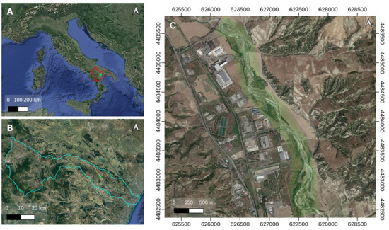
Figure 1.
Study area: (A) image highlighting the Basilicata region (red boundaries) in southern Italy and the location of the area analyzed (green dot); (B) Focus of the catchment area of the Basento river (light blue boundaries) and the location of the river reach investigated (green dot); (C) UAV surveyed area of the Basento river reach near the industrial area of Ferrandina (MT) (green polygon). The base map for all images is Google Earth.
The hydrological regime of the river follows the seasonal trend of the rainfall (mean annual rainfall about 766 mm with major events recorded between October and March), which shows the relationship between rainfall and river flow: maximum values between November and January, and minimum in July or August, with an average annual flow rate of 12.2 m3/s [54].
Specifically, the area under examination is subject to hydro-geomorphological high-risk: significant morphological changes have been recorded in the past [55], leading to several failures including the collapse of a road along its riverbank.
2.2. Data
In order to identify a universal and efficient automatic river features extraction approach from multitemporal aerial images, UAV image sequences of a river reach were collected in different seasons (June 2019, July 2020, October 2021 and March 2022), and with different weather conditions (sunny and cloudy). In this way, we considered a wide range of conditions that might affect the image quality (e.g., the reflectivity of water bodies, in sunny condition and the presence of shadows) and the river’s seasonal changes (e.g., flow rate and sediment load carried, which might affect water-color shades). In June 2019 and July 2020, river conditions in lean period were recorded, while in October 2021 and March 2022, river conditions during a flood period were recorded (following the hydrological regime of the river shown in Section 2.1).
The UAV images acquisition was carried out by using a DJI Inspire 2 (specifications at [56]) equipped with optical sensor DJI Zenmuse X5S (specifications at [57]), with a flying height of 50 m AGL of take-off location, nadir camera angle, images forward and side overlap of 85% and 65%, respectively. The UAV flight missions were set up with a single grid path using the “follow topography” option of Litchi (UAV flight mission planning app) to ensure a constant Ground Sampling Distance (GSD) of the images. Each flight mission consists of 9 strips (perpendicular to the main river path) with a length of about 160 m. The images were taken as RGB with a GSD of 1.09 cm/pix. In 2019 and 2021, about 3000 images were collected, in 2020 and 2022 about 4000 images.
The acquired datasets were processed using the Pix4D software v.4.7.5 (which follows the principles of SfM, as described in [58]), for generating RGB orthomosaics with an original resolution of 1.3 cm/pix (file size of about 6 GB) and positional accuracy ranging from 1 to 2 cm of RMSE values (using Manual Tie Points in addition to Ground Control Points uniformly distributed over the entire investigated area taking into account the geomorphological features). To analyze the resulting orthomosaics with TWS, due to the limited computing resources of our workstation (HP Z2 SFF G9 with 12 core Intel® Core™ i7 12,700 12th Generation, RAM 32 GB DDR5 – HP Store, Italy), a down-sampling of the resolution to 17 cm/pix (file size of about 60 MB) was performed (Figure 2), as a result of a trial-and-error method to find the resolution needed to run the entire classification workflow without complications.
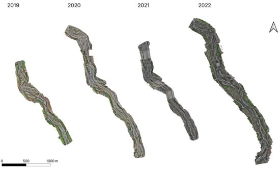
Figure 2.
Orthomosaics covering different lengths of reach of the Basento river, generated by UAV images acquired in different time interval (2019, 2020, 2021 and 2022) and with different weather conditions (sunny and cloudy).
2.3. Methods
The methodology presented in this paper consists of a sequence of steps. First, UAV multitemporal RGB orthomosaics are generated (see Section 2.2). Then, the classes to be extracted are defined: water, terrain, dense vegetation and background. Next, some training data for each class (set of pixels marked manually by the user exclusively over the orthomosaic 2021, because of the high variability of weather conditions and color hues of the classes, see Figure 2) are selected, specifically 188 pixels, as input for the TWS pixel-based segmentation algorithm.
TWS was set up with nine specific combinations of classifiers and image filters (representing training features, which are the key to the machine learning procedure). Each classifier was combined with the filters: BN + SF, BN + DoG, BN + SF + DoG; RF + SF, RF + DoG, RF + SF + DoG; kNN + SF, kNN + DoG, kNN + SF + DoG.
SF is a gradient-based edge detection filter. By applying two kernels, it computes an approximation of the gradient of the image intensity at each point, finding the direction along which there is the maximum increase from light to dark, the rate at which the change occurs along this direction and the probability of that part of image to represent an edge [59].
DoG is an image feature enhancement filter used for increasing the visibility of the edges. The method consists of subtracting two Gaussian images, where a kernel has a standard deviation smaller than the previous one. The convolution between the subtraction of kernels and the input image results in the edge detection of the image [60].
RF is an ensemble classifier, which uses a randomly selected subset of training variables and samples to generate several decision trees. Each tree casts a unique vote for the most popular class to classify input data [61].
BN is a classifier network, which computes a probability that indicates how likely the object belongs to a class. Each node of the network (direct acyclic graph) has a conditional probability distribution, and the object is assigned to the class in which the highest probability was calculated. Because the probability is calculated in terms of all features, each feature is able to play a role in the classification process [62].
Moreover, kNN is a nonparametric supervised learning classifier, which uses proximity to make classification or prediction about the clustering of a single data point. It identifies the nearest neighbor of a given point by determining the Euclidean distance between the query point and other data points [34].
Once the classifiers have been trained (on the original image and on its filtered version) and saved for each combination, they are used to classify the rest of the input pixels for the 2021 orthomosaic and all image pixels for 2019, 2020 and 2022 orthomosaics, using the same training data.
The outputs resulting from the application of each combination are a classified image (showing all the classes identified) and probability maps (gray-scale images, containing the probability that each pixel belongs to each class). The probability maps containing exclusively the water class (the class of greatest interest in the river flood monitoring perspective) are then transformed into binary ones by using the automatic binary segmentation tool of Fiji. This tool analyzes the histogram of the entire image and divides it into foreground objects and background, by taking an initial threshold and then calculating the averages of the pixels below and above the threshold. The averages of those two values are computed, the threshold is incremented, and the process is repeated until the threshold is larger than the composite average: threshold = (average background + average objects)/2. In this way, the area of the segmented class can be derived from the binary image, by applying a threshold in Fiji to select foreground pixels (with 255 value), and compared to the area obtained by the user manual digitization of the class in GIS environment (assumed as ground truth). Specifically, the comparison of the water class area, derived from automatic classification and user digitization, is made by considering the water class area strictly covering the riverbed. Then the misclassified water class area, over the whole image of the probability maps, is determined. All the steps listed above are shown in Figure 3.
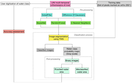
Figure 3.
Scheme of the main steps of the automatic river features extraction approach. The box in magenta indicates the process of generating UAV multi-temporal orthomosaics; the boxes in light blue indicate the filters used in combination with classifiers (green boxes) in the pre-processing phase; the classification process includes the box in yellow, which indicates the image segmentation process in TWS by leveraging the training data (light gray box at the top right) and the derived outputs (light gray boxes); the boxes in light green indicate all the post-processing operations applied to the probability maps (make binary images, calculation of riverbed water area and misclassified water area); the box in orange indicate the accuracy assessment phase of the classified and digitized (white box) riverbed water-class area.
2.4. Accuracy Estimation
To estimate the accuracy of the applied method, (a) a measure of the performance of the classifier for each combination and, (b) a measure of the accuracy between the classified and digitized water class (orthomosaic human interpretation), were carried out.
- (a)
- In this accuracy estimation, a confusion matrix was used to determine the metrics for each combination: accuracy (ACC; TP and TN indicate True Positives and True Negatives; FP and FN indicate False Positives and False Negatives) expressed in % (1), misclassification rate (ERR) expressed in % (2), precision (PR) expressed in weighted average (3), recall expressed in weighted average (4), F-measure (FM) weighted average (5) and kappa statistic (kappa) with expected accuracy (Exp ACC) (6).
- (b)
- The percentage error (7) between classified and digitized water class area covering the riverbed was determined for each combination, to measure the accuracy of True Positive (TP) reconstruction.
Furthermore, the misclassified water class area over the whole probability maps (subtracted by the area covering the riverbed, TP) was calculated for each combination, to measure the accuracy considering the False Positives (FP). In order to compare the values for each orthomosaic due to their different size, the percentage ratio (pMWA) of the misclassified water class area to the total image area (i.e., all pixels of the orthomosaics with not null values) was determined (8).
3. Results
In order to judge the performance of each combination (classifier plus image filter), with respect to the training data of each class marked exclusively on orthomosaic 2021, the metrics (see Section 2.4) were determined and compared, as shown in Table 1. Considering the values of all metrics, the combinations that showed the best performance were RF + DoG and kNN + DoG. Each combination was applied to the UAV multitemporal orthomosaics (see Figure 2) for generating the classified images including all classes (water, terrain, dense vegetation, background) and the probability maps of water class (the class of greatest interest in river flood monitoring perspective), as shown in Figure 4 and Figure 5, respectively. Based on preliminary visual analysis focusing mainly on the classification of water class, the best results were obtained with RF + SF and RF + SF + DoG.

Table 1.
Performance metrics values for each combination (classifier plus image filter).
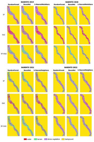
Figure 4.
Classified images showing the water, terrain, dense vegetation and background classes, generated by each combination (classifier plus image filter) and for each orthomosaic (2019, 2020, 2021, 2022).
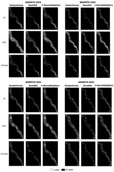
Figure 5.
Binary probability maps showing the water class generated by each combination (classifier plus image filter) and for each orthomosaic (2019, 2020, 2021, 2022).
Based on a quantitative analysis of the accuracy of the water class area obtained by automatic classification compared to manual digitization (Figure 6), in some cases the best results were quite different with respect to the preliminary visual analysis, considering both (a) the water class area covering the riverbed (TP) and (b) the misclassified water class area identified (FP) (following the methodologies reported in Section 2.4).
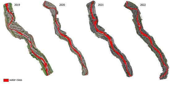
Figure 6.
Orthomosaics of a reach of the Basento river generated by UAV images acquired in different time interval (2019, 2020, 2021 and 2022) and with different weather conditions (sunny and cloudy). In red is shown the manually digitized water class area.
- (a)
- In this analysis, the best results were obtained by using RF + SF + DoG for the 2019 and 2022 orthomosaics, while kNN + DoG for the 2020 and 2021 orthomosaics, with percentage error values ranging from 12% to 20% (Table 2). The lowest percentage error, 12.49%, was recorded with kNN + DoG for the 2020 orthomosaic, and the highest, 70.37%, with BN + DoG for the 2022 orthomosaic (see Table 2 and Figure 7).
Table 2. Water area in riverbed (TP) and percentage error values between classified and digitized water class area covering the riverbed were calculated for each combination and the different orthomosaics.
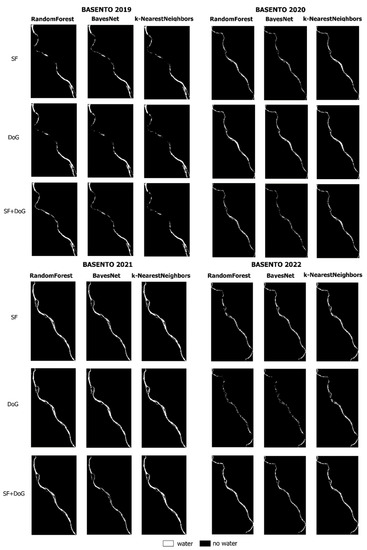 Figure 7. Binary probability maps showing the water class covering exclusively the riverbed area, generated by each combination (classifier plus image filter) and for each orthomosaic (2019, 2020, 2021, 2022).
 - (b)
- The best results were obtained by using BN + SF + DoG for the 2019 and 2022 orthomosaics, and BN + SF for the 2020 and 2021 orthomosaics, with percentage values ranging from 0.70% to 2.13% (Table 3). The lowest value, 0.70%, was recorded with BN + SF for the 2021 orthomosaic, and the highest, 34.16%, with RF + DoG for the 2019 orthomosaic (see Table 3 and Figure 8).
Table 3. Misclassified water class area values (FP) and percentage ratio values between FP water area and total image area were calculated for each combination (classifier plus image filter) and the different orthomosaics.
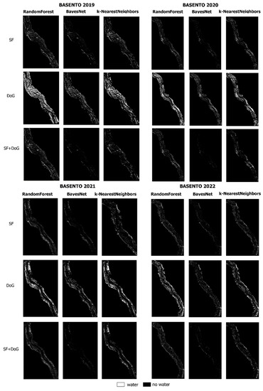 Figure 8. Binary probability maps showing the misclassified water class over the whole image, generated by each combination (classifier plus image filter) and for the different orthomosaics (2019, 2020, 2021, 2022).
4. Discussion
Analyses of the water-class accuracy classification revealed that the best results are not consistent in all cases with the performance values of the combinations of classifiers plus image filters (see Section 3). In fact, despite the fact that the best-performing combinations were RF + DoG and kNN + DoG, considering the riverbed water class area accuracy analysis, for the 2019 and 2020 orthomosaics the best results were obtained by Random Forest, with different filter combinations RF + SF + DoG, while for the 2020 and 2021 orthomosaics, the results were consistent with the performance values. This situation was corroborated by the results of the misclassified water-class area accuracy analysis: the best results, indeed, were obtained by BN + SF for the 2020 and 2021 orthomosaics, and by BN + SF + DoG for the 2019 and 2022 orthomosaics. This behavior is mainly related to the training dataset used for the classification (a small set of pixels extracted exclusively from the 2021 orthomosaic, which was also used to classify 2019, 2020, and 2022 orthomosaics), on test data with different conditions. Water-class color hues due to both different weather conditions and the date of UAV image acquisition (lean and high discharge periods of the river, affecting water flow and sediment load), indeed, may lead to slightly different results.
Based on the results of the riverbed water-class area accuracy analysis (TP accuracy analysis), the combination that led to better classification was RF + SF + DoG for the 2019 and 2022 orthomosaics, and kNN + DoG for the 2020 and 2021 orthomosaics. This behavior was probably due to the different amount and color hue of water in the riverbed (ongoing study).
The results of the misclassified water-class area accuracy analysis (FP accuracy analysis) showed the same behavior for the 2020 and 2021 orthomosaics, with the best results with BN + SF, and for the 2019 and 2022 orthomosaics, the best results were with BN + SF + DoG. This behavior resulted in the inference that BN + SF works well in the presence of less vegetation (percentage values of 0.87% and 0.70%, for the 2020 and 2021 orthomosaics, respectively), while BN + SF + DoG works well in the presence of greater vegetation (percentage values of 2.13% and 1.49%, for the 2019 and 2022 orthomosaics, respectively). This result was validated by an analysis of the amount of vegetation present in the different orthomosaics, by determining the ENDVI (vis) index (assumed as ground truth for the identification of vegetation [63]) and the ratio of the resulting vegetation area to the total image area for each orthomosaic (Table 4). This index turns out to be an adaptation of the classical ENDVI index (developed by LDP LLC, Carlstadt, NJ, USA [64]) to the bands of the visible. The results confirmed a higher presence of vegetation for the 2019 and 2022 orthomosaics with values of 5.8% and 2.8%, respectively (see Table 4). Vegetation is the mostly misclassified class as the water class (as also stated in [39]) because it can show greater variability in color hues according to the different seasons.
Table 4.
Amount of vegetation determined by the ENDVI(vis) index, calculated for the different orthomosaics. The percentage values represent the ratio of the vegetation area to the total image area.
In order to indicate a universal combination for water-class identification, according to the different characteristics of the orthomosaics (2019, 2020, 2021, 2022), RF + SF + DoG could represent the best combination for water segmentation (more TP and less FP) considering all the values of both TP and FP reconstruction accuracy (Table 2 and Table 3, respectively). Considering the results obtained, the use of high-resolution, low-altitude and multi-temporal UAV imagery in combination with the supervised classification approach proved to be an efficient, cost-effective and prompt solution for the identification of water in riverine environments. Specifically, the advantage of acquiring on-demand images, recording the different quality conditions and the river’s seasonal changes, results in an improvement in the water classification process.
Despite the optimal results, the proposed approach presents some constraints that have partially affected the results and that could be overcome in a future perspective to improve the classification process. In particular, a limit of our approach could have been the use of a training dataset consisting of a small set of user-identified pixels on a specific orthomosaic; in this view, the use of more populated and variable training datasets could greatly improve the classification process. The use of multi and hyper-spectral UAV images in addition to RGB could also improve the classification process, by recognizing ground objects that may have very similar features (we have seen how using RGB imagery the vegetation is often misclassified as water, as it may present similar color hues). The assumption of a manually digitized water class as ground truth may represent a limit, indeed the operator may run into a misclassification error as in the case of identifying wetlands. Another limit of this approach consists in the analysis of UAV orthomosaics at original resolution in Fiji with TWS: the large size (order of magnitude of one GB) and the low computational resources of a traditional workstation, result in the need to down-scale the original data (in this case from 1.3 cm/pix with a file size about 6 GB, to 17 cm/pix with a file size about 60 MB). The down-scaling could be overcome by using the high-performance computing (HPC) paradigm. Taking advantage of the near-unlimited computing resources of computing cluster by parallel computing, for example, it is possible to divide the very high-resolution orthomosaic into tiles and to apply the classification workflow for each of them in parallel on a single server, eventually merging the results obtained by each server. This could result in an exponentially reduced processing time (crucial in emergency scenarios) and in the ability to analyze increasingly large river reaches with unprecedented levels of detail.
Finally, a combination of methods using all the outputs generated by UAV surveys (dense point cloud, digital terrain model and digital surface model) or Lidar sensor data could improve the classification of both terrain and vegetation classes, which could help to identify the water class accurately.
Notwithstanding the above limitations, our approach for automatic river features extraction represents an efficient tool that provides results very close to the human interpretation and, therefore, could prove to be a key element for improving the hydro-geomorphological and flooding hazard assessment in riverine environments. The proposed approach represents an important contribution to the management activities of flood-prone environments, especially in view of sudden climate changes, as it ensures a reduction of time in the image analysis and accurate and rapid identification of flood-affected areas immediately after the calamitous event. Therefore, this approach enhances the post-disaster damage estimation, which facilitates the intervention of military corps and civil protection, and enables the implementation of recovery plans, also for insurance purposes.
5. Conclusions
The present work compared the accuracy of different combinations (classifier plus image filter) using TWS, with respect to human photo-interpretation, in order to identify an effective open-source supervised approach for automatic water-class extraction from UAV multitemporal orthomosaics of wide areas of riverine environments.
TWS was set up with 9 specific combinations of classifiers and image filters: RF + SF, RF + DoG, RF + SF + DoG; BN + SF, BN + DoG, BN + SF + DoG; kNN + SF, kNN + DoG, kNN + SF + DoG.
Performance metrics values for each combination were determined with respect to the training data of each class (water, terrain, dense vegetation and background) extracted from the 2021 orthomosaic. The accuracy values recorded ranged from about 93% to about 97%, while the misclassification rate values ranged from about 2% to about 6%.
The accuracy of the water class was determined by (a) comparing the classified and digitized water-class area covering the riverbed, and by (b) determining the misclassified water-class area over the whole probability maps. In (a), the best results were obtained by using RF + SF + DoG for the 2019 and 2022 orthomosaics, while kNN + DoG for the 2020 and 2021 orthomosaics, with percentage errors of the comparison between classified and digitized riverbed water-class area, ranging from 12% to 20%. In (b) the best results were obtained by using BN + SF + DoG for the 2019 and 2022 orthomosaics, and BN + SF for the 2020 and 2021 orthomosaics, with percentage values of the ratio between misclassified water area and total image area, ranging from 0.70% to 2.13%.
According to the different characteristics of the analyzed orthomosaics and the results obtained from the water class accuracy analyses, RF + SF + DoG could represent the best combination for water segmentation (more TP and less FP).
The approach proposed in this work for automatic river water-class extraction represents an efficient tool that provides results very close to the human interpretation and, therefore, it could prove to be a valuable tool to support and improve the hydro-geomorphological and flooding hazard assessments in riverine environments.
Author Contributions
Conceptualization, M.L.S., R.C.; methodology, M.L.S., R.C., D.C., P.D.; software, M.L.S., R.C.; validation, M.L.S., R.C., D.C., P.D.; resources, D.C., P.D.; writing—original draft preparation, M.L.S., R.C.; writing—review and editing, M.L.S., R.C., P.D., D.C.; supervision, D.C., P.D. All authors have read and agreed to the published version of the manuscript.
Funding
This research received financial support from the project “RPASinAir—Integrazione dei Sistemi Aeromobili a Pilotaggio Remoto nello spazio aereo non segregato per servizi”, PON ricerca e innovazione 2014–2020; from the project “GeoScienceIR” funded by MIUR (missione 4 PNRR); and from the project “Centro Nazionale di Ricerca HPC, Big Data e Quantum Computing” -Piano Nazionale di Ripresa e Resilienza, Missione 4 Componente 2 Investimento 1.4 “Potenziamento strutture di ricerca e creazione di ‘campioni nazionali di R&S’ su alcune Key Enabling Technologies” funded by European Union—NextGenerationEU.
Data Availability Statement
Data are available from the authors upon request.
Acknowledgments
We thank Peter Ernest Wigand for the critical review and for the revision of the English language.
Conflicts of Interest
The authors declare no conflict of interest.
References
- Howard, A.J. Managing Global Heritage in the Face of Future Climate Change: The Importance of Understanding Geological and Geomorphological Processes and Hazards. Int. J. Herit. Stud. 2013, 19, 632–658. [Google Scholar] [CrossRef]
- Kuenzer, C.; Guo, H.; Huth, J.; Leinenkugel, P.; Li, X.; Dech, S. Flood Mapping and Flood Dynamics of the Mekong Delta: ENVISAT-ASAR-WSM Based Time Series Analyses. Remote Sens. 2013, 5, 687–715. [Google Scholar] [CrossRef]
- Feng, Q.; Liu, J.; Gong, J. Urban Flood Mapping Based on Unmanned Aerial Vehicle Remote Sensing and Random Forest Classifier—A Case of Yuyao, China. Water 2015, 7, 1437–1455. [Google Scholar] [CrossRef]
- Jonkman, S.N. Global Perspectives on Loss of Human Life Caused by Floods. Nat. Hazards 2005, 34, 151–175. [Google Scholar] [CrossRef]
- Grove, J.R.; Croke, J.; Thompson, C. Quantifying Different Riverbank Erosion Processes during an Extreme Flood Event. Earth Surf. Process. Landf. 2013, 38, 1393–1406. [Google Scholar] [CrossRef]
- Duong, T.T.; Komine, H.; Do, M.D.; Murakami, S. Riverbank Stability Assessment under Flooding Conditions in the Red River of Hanoi, Vietnam. Comput. Geotech. 2014, 61, 178–189. [Google Scholar] [CrossRef]
- Akay, S.S.; Özcan, O.; Şanlı, F.B. Quantification and Visualization of Flood-Induced Morphological Changes in Meander Structures by UAV-Based Monitoring. Eng. Sci. Technol. Int. J. 2022, 27, 101016. [Google Scholar] [CrossRef]
- Mathew, A.E.; Kumar, S.S.; Vivek, G.; Iyyappan, M.; Karthikaa, R.; Kumar, P.D.; Dash, S.K.; Gopinath, G.; Usha, T. Flood Impact Assessment Using Field Investigations and Post-Flood Survey. J. Earth Syst. Sci. 2021, 130, 147. [Google Scholar] [CrossRef]
- Chandler, J.; Ashmore, P.; Paola, C.; Gooch, M.; Varkaris, F. Monitoring River-Channel Change Using Terrestrial Oblique Digital Imagery and Automated Digital Photogrammetry. Ann. Assoc. Am. Geogr. 2002, 92, 631–644. [Google Scholar] [CrossRef]
- Tanim, A.H.; McRae, C.B.; Tavakol-Davani, H.; Goharian, E. Flood Detection in Urban Areas Using Satellite Imagery and Machine Learning. Water 2022, 14, 1140. [Google Scholar] [CrossRef]
- Annis, A.; Nardi, F.; Castelli, F. Simultaneous Assimilation of Water Levels from River Gauges and Satellite Flood Maps for Near-Real-Time Flood Mapping. Hydrol. Earth Syst. Sci. 2022, 26, 1019–1041. [Google Scholar] [CrossRef]
- Ansari, E.; Akhtar, M.N.; Bakar, E.A.; Uchiyama, N.; Kamaruddin, N.M.; Umar, S.N.H. Investigation of Geomorphological Features of Kerian River Using Satellite Images. In Proceedings of the Intelligent Manufacturing and Mechatronics; Perlis, Malaysia, 10 August 2020, Bahari, M.S., Harun, A., Zainal Abidin, Z., Hamidon, R., Zakaria, S., Eds.; Springer: Singapore, 2021; pp. 91–101. [Google Scholar]
- Jung, Y.; Kim, D.; Kim, D.; Kim, M.; Lee, S.O. Simplified Flood Inundation Mapping Based On Flood Elevation-Discharge Rating Curves Using Satellite Images in Gauged Watersheds. Water 2014, 6, 1280–1299. [Google Scholar] [CrossRef]
- Refice, A.; D’Addabbo, A.; Capolongo, D. Methods, Techniques and Sensors for Precision Flood Monitoring Through Remote Sensing. In Flood Monitoring through Remote Sensing; Refice, A., D’Addabbo, A., Capolongo, D., Eds.; Springer Remote Sensing/Photogrammetry; Springer International Publishing: Cham, Switzerland, 2018; pp. 1–25. ISBN 978-3-319-63959-8. [Google Scholar]
- Refice, A.; Capolongo, D.; Chini, M.; D’Addabbo, A. Improving Flood Detection and Monitoring through Remote Sensing. Water 2022, 14, 364. [Google Scholar] [CrossRef]
- Colacicco, R.; Refice, A.; Nutricato, R.; D’Addabbo, A.; Nitti, D.O.; Capolongo, D. High Spatial and Temporal Resolution Flood Monitoring through Integration of Multisensor Remotely Sensed Data and Google Earth Engine Processing. In Proceedings of the EGU General Assembly 2022, Vienna, Austria, 23–27 May 2022. [Google Scholar] [CrossRef]
- Yan, X.; Xu, K.; Feng, W.; Chen, J. A Rapid Prediction Model of Urban Flood Inundation in a High-Risk Area Coupling Machine Learning and Numerical Simulation Approaches. Int. J. Disaster Risk Sci. 2021, 12, 903–918. [Google Scholar] [CrossRef]
- Ayoub, V.; Delenne, C.; Chini, M.; Finaud-Guyot, P.; Mason, D.; Matgen, P.; Maria-Pelich, R.; Hostache, R. A Porosity-Based Flood Inundation Modelling Approach for Enabling Faster Large Scale Simulations. Adv. Water Resour. 2022, 162, 104141. [Google Scholar] [CrossRef]
- Winsemius, H.C.; Van Beek, L.P.H.; Jongman, B.; Ward, P.J.; Bouwman, A. A Framework for Global River Flood Risk Assessments. Hydrol. Earth Syst. Sci. 2013, 17, 1871–1892. [Google Scholar] [CrossRef]
- Nandalal, K.D.W. Use of a Hydrodynamic Model to Forecast Floods of Kalu River in Sri Lanka. J. Flood Risk Manag. 2009, 2, 151–158. [Google Scholar] [CrossRef]
- La Salandra, M.; Miniello, G.; Nicotri, S.; Italiano, A.; Donvito, G.; Maggi, G.; Dellino, P.; Capolongo, D. Generating UAV High-Resolution Topographic Data within a FOSS Photogrammetric Workflow Using High-Performance Computing Clusters. Int. J. Appl. Earth Obs. Geoinf. 2021, 105, 102600. [Google Scholar] [CrossRef]
- Ansari, E.; Akhtar, M.N.; Abdullah, M.N.; Othman, W.A.F.W.; Bakar, E.A.; Hawary, A.F.; Alhady, S.S.N. Image Processing of UAV Imagery for River Feature Recognition of Kerian River, Malaysia. Sustainability 2021, 13, 9568. [Google Scholar] [CrossRef]
- Rivas Casado, M.; Ballesteros Gonzalez, R.; Kriechbaumer, T.; Veal, A. Automated Identification of River Hydromorphological Features Using UAV High Resolution Aerial Imagery. Sensors 2015, 15, 27969–27989. [Google Scholar] [CrossRef]
- Hemmelder, S.; Marra, W.; Markies, H.; De Jong, S.M. Monitoring River Morphology & Bank Erosion Using UAV Imagery—A Case Study of the River Buëch, Hautes-Alpes, France. Int. J. Appl. Earth Obs. Geoinf. 2018, 73, 428–437. [Google Scholar] [CrossRef]
- La Salandra, M.; Roseto, R.; Mele, D.; Dellino, P.; Capolongo, D. Probabilistic Hydro-Geomorphological Hazard Assessment Based on UAV-Derived High-Resolution Topographic Data: The Case of Basento River (Southern Italy). Sci. Total Environ. 2022, 842, 156736. [Google Scholar] [CrossRef] [PubMed]
- Zingaro, M.; La Salandra, M.; Capolongo, D. New Perspectives of Earth Surface Remote Detection for Hydro-Geomorphological Monitoring of Rivers. Sustainability 2022, 14, 14093. [Google Scholar] [CrossRef]
- Ezequiel, C.A.F.; Cua, M.; Libatique, N.C.; Tangonan, G.L.; Alampay, R.; Labuguen, R.T.; Favila, C.M.; Honrado, J.L.E.; Caños, V.; Devaney, C.; et al. UAV Aerial Imaging Applications for Post-Disaster Assessment, Environmental Management and Infrastructure Development. In Proceedings of the 2014 International Conference on Unmanned Aircraft Systems (ICUAS), Orlando, FL, USA, 27–30 May 2014; pp. 274–283. [Google Scholar]
- Munawar, H.S.; Hammad, A.W.A.; Waller, S.T.; Thaheem, M.J.; Shrestha, A. An Integrated Approach for Post-Disaster Flood Management Via the Use of Cutting-Edge Technologies and UAVs: A Review. Sustainability 2021, 13, 7925. [Google Scholar] [CrossRef]
- Maxwell, A.E.; Warner, T.A.; Fang, F. Implementation of Machine-Learning Classification in Remote Sensing: An Applied Review. Int. J. Remote Sens. 2018, 39, 2784–2817. [Google Scholar] [CrossRef]
- Senthilnath, J.; Bajpai, S.; Omkar, S.N.; Diwakar, P.G.; Mani, V. An Approach to Multi-Temporal MODIS Image Analysis Using Image Classification and Segmentation. Adv. Space Res. 2012, 50, 1274–1287. [Google Scholar] [CrossRef]
- Moortgat, J.; Li, Z.; Durand, M.; Howat, I.; Yadav, B.; Dai, C. Deep Learning Models for River Classification at Sub-Meter Resolutions from Multispectral and Panchromatic Commercial Satellite Imagery. Remote Sens. Environ. 2022, 282, 113279. [Google Scholar] [CrossRef]
- Boston, T.; Van Dijk, A.; Larraondo, P.R.; Thackway, R. Comparing CNNs and Random Forests for Landsat Image Segmentation Trained on a Large Proxy Land Cover Dataset. Remote Sens. 2022, 14, 3396. [Google Scholar] [CrossRef]
- Al-Ghrairi, A.H.T.; Abed, Z.H.; Fadhil, F.H. Classification of Satellite Images Based on Color Features Using Remote Sensing. Int. J. Comput. IJC 2018, 31, 11. [Google Scholar]
- Thanh Noi, P.; Kappas, M. Comparison of Random Forest, k-Nearest Neighbor, and Support Vector Machine Classifiers for Land Cover Classification Using Sentinel-2 Imagery. Sensors 2018, 18, 18. [Google Scholar] [CrossRef]
- Van Iersel, W.; Straatsma, M.; Middelkoop, H.; Addink, E. Multitemporal Classification of River Floodplain Vegetation Using Time Series of UAV Images. Remote Sens. 2018, 10, 1144. [Google Scholar] [CrossRef]
- Oga, T.; Harakawa, R.; Minewaki, S.; Umeki, Y.; Matsuda, Y.; Iwahashi, M. River State Classification Combining Patch-Based Processing and CNN. PLoS ONE 2020, 15, e0243073. [Google Scholar] [CrossRef]
- Ibrahim, N.S.; Sharun, S.M.; Osman, M.K.; Mohamed, S.B.; Abdullah, S.H.Y.S. The Application of UAV Images in Flood Detection Using Image Segmentation Techniques. Indones. J. Electr. Eng. Comput. Sci. 2021, 23, 1219. [Google Scholar] [CrossRef]
- Munawar, H.S.; Hammad, A.W.A.; Waller, S.T. A Review on Flood Management Technologies Related to Image Processing and Machine Learning. Autom. Constr. 2021, 132, 103916. [Google Scholar] [CrossRef]
- Miniello, G.; La Salandra, M.; Vino, G. Deep Neural Networks for Remote Sensing Image Classification. In Proceedings of the Intelligent Computing, 14–15 July 2022; Arai, K., Ed.; Springer International Publishing: Cham, Switzerland, 2022; pp. 117–128. [Google Scholar]
- Teodoro, A.C.; Araujo, R. Comparison of Performance of Object-Based Image Analysis Techniques Available in Open Source Software (Spring and Orfeo Toolbox/Monteverdi) Considering Very High Spatial Resolution Data. J. Appl. Remote Sens. 2016, 10, 016011. [Google Scholar] [CrossRef]
- Horning, N.; Fleishman, E.; Ersts, P.J.; Fogarty, F.A.; Wohlfeil Zillig, M. Mapping of Land Cover with Open-Source Software and Ultra-High-Resolution Imagery Acquired with Unmanned Aerial Vehicles. Remote Sens. Ecol. Conserv. 2020, 6, 487–497. [Google Scholar] [CrossRef]
- Wyard, C.; Beaumont, B.; Grippa, T.; Hallot, E. UAV-Based Landfill Land Cover Mapping: Optimizing Data Acquisition and Open-Source Processing Protocols. Drones 2022, 6, 123. [Google Scholar] [CrossRef]
- Chabot, D.; Dillon, C.; Shemrock, A.; Weissflog, N.; Sager, E.P.S. An Object-Based Image Analysis Workflow for Monitoring Shallow-Water Aquatic Vegetation in Multispectral Drone Imagery. ISPRS Int. J. Geo-Inf. 2018, 7, 294. [Google Scholar] [CrossRef]
- Arganda-Carreras, I.; Kaynig, V.; Rueden, C.; Eliceiri, K.W.; Schindelin, J.; Cardona, A.; Sebastian Seung, H. Trainable Weka Segmentation: A Machine Learning Tool for Microscopy Pixel Classification. Bioinformatics 2017, 33, 2424–2426. [Google Scholar] [CrossRef]
- Schindelin, J.; Arganda-Carreras, I.; Frise, E.; Kaynig, V.; Longair, M.; Pietzsch, T.; Preibisch, S.; Rueden, C.; Saalfeld, S.; Schmid, B.; et al. Fiji: An Open-Source Platform for Biological-Image Analysis. Nat. Methods 2012, 9, 676–682. [Google Scholar] [CrossRef]
- Hart, N.H.; Huang, L. Monitoring Nests of Solitary Bees Using Image Processing Techniques. In Proceedings of the 2012 19th International Conference on Mechatronics and Machine Vision in Practice (M2VIP), Auckland, New Zealand, 28–30 November 2012; pp. 1–4. [Google Scholar]
- Dobens, A.C.; Dobens, L.L. FijiWings: An Open Source Toolkit for Semiautomated Morphometric Analysis of Insect Wings. G3: Genes Genomes Genet. 2013, 3, 1443–1449. [Google Scholar] [CrossRef]
- Krueger, M.A.; Huke, S.S.; Glenny, R.W. Visualizing Regional Myocardial Blood Flow in the Mouse. Circ. Res. 2013, 112, e88–e97. [Google Scholar] [CrossRef] [PubMed]
- Bohari, S.N.; Ahmad, A.; Talib, N.; Hajis, A.M.H.A. Accuracy Assessment of Automatic Road Features Extraction from Unmanned Autonomous Vehicle (UAV) Imagery. IOP Conf. Ser. Earth Environ. Sci. 2021, 767, 012028. [Google Scholar] [CrossRef]
- Abdollahi, A.; Pradhan, B.; Shukla, N. Extraction of Road Features from UAV Images Using a Novel Level Set Segmentation Approach. Int. J. Urban Sci. 2019, 23, 391–405. [Google Scholar] [CrossRef]
- Shojaei, A.; Moud, H.I.; Flood, I. Proof of Concept for the Use of Small Unmanned Surface Vehicle in Built Environment Management. In Proceedings of the Construction Research Congress 2018, New Orleans, LA, USA, 2–4 April 2018; American Society of Civil Engineers: New Orleans, LA, USA, 2018; pp. 116–126. [Google Scholar]
- Taugourdeau, S.; Dionisi, M.; Lascoste, M.; Lesnoff, M.; Capron, J.M.; Borne, F.; Borianne, P.; Julien, L. A First Attempt to Combine NIRS and Plenoptic Cameras for the Assessment of Grasslands Functional Diversity and Species Composition. Agriculture 2022, 12, 704. [Google Scholar] [CrossRef]
- Tropeano, M.; Cilumbriello, A.; Sabato, L.; Gallicchio, S.; Grippa, A.; Longhitano, S.G.; Bianca, M.; Gallipoli, M.R.; Mucciarelli, M.; Spilotro, G. Surface and Subsurface of the Metaponto Coastal Plain (Gulf of Taranto—Southern Italy): Present-Day- vs LGM-Landscape. Geomorphology 2013, 203, 115–131. [Google Scholar] [CrossRef]
- Piccarreta, M.; Pasini, A.; Capolongo, D.; Lazzari, M. Changes in Daily Precipitation Extremes in the Mediterranean from 1951 to 2010: The Basilicata Region, Southern Italy. Int. J. Climatol. 2013, 33, 3229–3248. [Google Scholar] [CrossRef]
- de Musso, N.M.; Capolongo, D.; Caldara, M.; Surian, N.; Pennetta, L. Channel Changes and Controlling Factors over the Past 150 Years in the Basento River (Southern Italy). Water 2020, 12, 307. [Google Scholar] [CrossRef]
- Available online: https://www.dji.com/it/inspire-2/info (accessed on 31 December 2022).
- Available online: https://www.dji.com/it/zenmuse-x5s/info (accessed on 31 December 2022).
- Eltner, A.; Sofia, G. Chapter 1-Structure from Motion Photogrammetric Technique. In Developments in Earth Surface Processes; Tarolli, P., Mudd, S.M., Eds.; Remote Sensing of Geomorphology; Elsevier: Amsterdam, The Netherlands, 2020; Volume 23, pp. 1–24. [Google Scholar]
- Bora, D. A Novel Approach for Color Image Edge Detection Using Multidirectional Sobel Filter on HSV Color Space. Int. J. Comput. Sci. Eng. 2017, 5, 154–159. [Google Scholar]
- Assirati, L.; Silva, N.R.; Berton, L.; Lopes, A.A.; Bruno, O.M. Performing Edge Detection by Difference of Gaussians Using Q-Gaussian Kernels. J. Phys. Conf. Ser. 2014, 490, 012020. [Google Scholar] [CrossRef]
- Pal, M. Random Forest Classifier for Remote Sensing Classification. Int. J. Remote Sens. 2005, 26, 217–222. [Google Scholar] [CrossRef]
- Kang, Z.; Yang, J.; Zhong, R. A Bayesian-Network-Based Classification Method Integrating Airborne LiDAR Data With Optical Images. IEEE J. Sel. Top. Appl. Earth Obs. Remote Sens. 2017, 10, 1651–1661. [Google Scholar] [CrossRef]
- Available online: https://www.esriitalia.it/media/sync/20210426_143037_StefanoMugnoliESRI2021_1.pdf (accessed on 12 December 2022).
- Available online: http://www.maxmax.com/endvi.htm (accessed on 12 December 2022).
Disclaimer/Publisher’s Note: The statements, opinions and data contained in all publications are solely those of the individual author(s) and contributor(s) and not of MDPI and/or the editor(s). MDPI and/or the editor(s) disclaim responsibility for any injury to people or property resulting from any ideas, methods, instructions or products referred to in the content. |
© 2023 by the authors. Licensee MDPI, Basel, Switzerland. This article is an open access article distributed under the terms and conditions of the Creative Commons Attribution (CC BY) license (https://creativecommons.org/licenses/by/4.0/).