Event-Triggered Hierarchical Planner for Autonomous Navigation in Unknown Environment

Abstract

End-to-end deep neural network (DNN)-based motion planners have shown great potential in high-speed autonomous UAV flight. Yet, most existing methods only employ a single high-capacity DNN, which typically lacks generalization ability and suffers from high sample complexity. We propose a novel event-triggered hierarchical planner (ETHP), which exploits the bi-level optimization nature of the navigation task to achieve both efficient training and improved optimality. Specifically, we learn a depth-image-based end-to-end motion planner in a hierarchical reinforcement learning framework, where the high-level DNN is a reactive collision avoidance rerouter triggered by the clearance distance, and the low-level DNN is a goal-chaser that generates the heading and velocity references in real time. Our training considers the field-of-view constraint and explores the bi-level structural flexibility to promote the spatio–temporal optimality of planning. Moreover, we design simple yet effective rules to collect hindsight experience replay buffers, yielding more high-quality samples and faster convergence. The experiments show that, compared with a single-DNN baseline planner, ETHP significantly improves the success rate and generalizes better to the unseen environment.

1. Introduction

Autonomous navigation with collision avoidance plays a critical role in the safe operation of UAVs in unknown environments [1,2,3,4]. It is a challenging task since UAVs typically have limited onboard sensing and computing ability, and the environmental information can only be perceived locally. Common model-based navigation stacks follow the sensing–mapping–planning pipeline [5], which is robust and highly interpretable. However, each of these subtasks can be computationally demanding for onboard computation and introduces significant latency that limits the flight speed and range.

End-to-end deep neural network (DNN)-based methods show great promise in developing portable onboard navigation solutions for autonomous flight [6,7,8,9,10,11]. Compared with the traditional methods, the end-to-end DNN policy directly maps the raw sensing inputs to navigation commands, skipping the mapping and many other intermediate heavy processings [8]. The DNN policies are commonly trained under the frameworks of imitation learning or reinforcement learning. Imitation-learning-based methods directly copy from human experience [11] or expert algorithms [8], which lack the potential to achieve better optimality. It is generally more difficult to train with reinforcement learning due to the lack of supervision [9,10]. Efficient training with reinforcement learning requires “good” data, which are those with high rewards, sufficient exploration of the environment, and somewhat representative of a good policy. However, such good data are scarce when learning from scratch, as collisions happen most of the time at the beginning of the training. In addition, the aforementioned deep-learning-based methods all utilize a single high-capacity DNN, which has relatively poor generalization ability.

In this paper, we view the navigation task as a bi-level optimization problem, which naturally consists of two goals: reaching the goal point and avoiding collisions along the way. This structural property is exploited to improve the design of the DNN policy. Specifically, we propose an event-triggered hierarchical reinforcement learning-based planner for autonomous navigation. Different from other end-to-end learning-based methods, we train two DNNs to focus separately on goal reaching and collision avoidance, respectively (see Figure 1). In contrast to conventional hierarchical-based reinforcement learning [12], we set different reward functions for the two levels to guide them to respond to obstacles and waypoints, respectively. We consider navigation in unknown environments using a depth camera. Hence, only local perception measurements with limited field-of-view are utilized. Furthermore, we design the high-level policy to activate only if obstacles occur in the range of the field of view. This event-triggered mechanism improves the training efficiency and success rate by reducing the chance of generating wrong subgoals. On the training aspect, the bi-level structure provides additional flexibility and improved efficiency as it allows the reuse of data for the training of both DNNs, despite their different objectives. In particular, we develop effective rules to generate good samples using the hindsight transitions experience [13] for both levels of policies, which significantly improves the training efficiency and optimality.

Overall, the proposed event-triggered reactive planning offers a simple yet efficient collision avoidance navigation strategy. To our knowledge, this is the first time hierarchical reinforcement learning has been successfully applied to UAV autonomous navigation. We conduct extensive simulations to demonstrate the significant performance improvement over baseline single-DNN policies trained with state-of-the-art reinforcement algorithms under similar settings. We also demonstrate the generalization to unseen and more complex environments. Moreover, the real flight test shows that the proposed planner has the potential to engender spatio–temporally optimized paths, which is generally difficult for traditional model-based or imitation-learning-based methods.

2. Preliminaries

We briefly review the basics of hierarchical reinforcement learning, hindsight transitions experience, and deep deterministic policy gradient algorithms below.

2.1. Hierarchical Reinforcement Learning

Hierarchical reinforcement learning (HRL) decomposes the challenging long-horizon decision-making task into simpler subtasks of different objectives [14]. In reinforcement learning, which is based on the assumption of the Markov decision process (MDP) [15], only the sequential nature of the decision process is relevant, and the amount of time that passes between decision stages is ignored. Different from that, most of the HRL approaches are based on the assumption of the semi-Markov decision process (SMDP) [16], where the system is treated as remaining in each state for a random waiting time. Following SMDP, the Bellman equations are set as:

$$V\left(s\right)=\underset{a\in A_s}{max}\left[R(s,a)+\sum _{s^{\prime },\tau }{\gamma }^{\tau }P\left(s^{\prime },\tau \mid s,a\right)V\left(s^{\prime }\right)\right],$$

(1)

and:

$$Q(s,a)=R(s,a)+\sum _{s^{\prime },\tau }{\gamma }^{\tau }P\left(s^{\prime },\tau \mid s,a\right)\underset{a^{\prime }\in A_{s^{\prime }}}{max}Q\left(s^{\prime },a^{\prime }\right)$$

(2)

where the random variable $\tau$ denotes the waiting time for state s when action a is executed. The transition probabilities generalize to give the joint probability that a transition from state s to state $s^{\prime }$ occurs after $\tau$ time steps when action a is executed.

A few different HRL frameworks have been proposed in the literature [12,17,18,19,20,21,22]. Among them, the goal-reach-based method provides stronger explainability for HRL [20]. This type of method expands the original $V\left(s\right)$ and $Q(s,a)$ into $V(s,g)$ and $Q(s,g,a)$, respectively. The higher-level policy of the goal-reach-based method generates subgoals with specific physical meanings for the lower-level policy to execute. Particularly, in many applications, the state space of the lower-level policy is designed conveniently to be the same as the action space of the higher-level policy [12,20,21,22,23].

In HRL, the policies at different levels are coupled. The lower-level policies are constantly updated during training. This essentially results in a non-stationary environment for training the higher-level policy, since the rewards received by the higher-level policies depend on the lower-level policies’ changing behaviors. Consequently, the training of HRL is typically very difficult. To improve training efficiency, the idea of Hindsight Experience Replay (HER) [13] is utilized to generate sufficient “good” samples for training the multi-level policies in HRL. In particular, hindsight transitions were first applied to HRL in the work of Hierarchical Actor-Critic (HAC) [12], where the experience replay samples are modified in a way that decouples the tasks of different levels. The samples are effectively re-purposed to contribute to more efficient training. We explain in more detail in the following subsection.

2.2. Hindsight Transitions Experience

Off-policy reinforcement learning algorithms commonly utilize the experience replay buffer to update the parameters more stably and efficiently. When the target in the training environment is difficult to achieve, there can be insufficient good samples in the experience replay buffer for effective training. This is especially the case for sparse-reward tasks, where experiences that are conducive to learning are scarce. Hindsight goal transition mitigates this problem by replacing the target with the agent’s current state:

$$\begin{array}{c}\hfill [stat{e}_{initial}=>s_0,action=>a_1,reward=>R,stat{e}_{next}=>s_1,goa{l}_{sub}=>s_1]\end{array}$$

(3)

where the $goa{l}_{sub}$ generated by the high-level policy is forced to set as $s_1$, such that the low-level policy is better rewarded from the environment, which significantly improves the training efficiency.

As briefly mentioned in the last subsection, there exists a non-stationary issue faced by the higher-level policy for the off-policy HRL method. For example, since the lower-level policy is constantly changing while training, a sample observed for a certain high-level action in the past may not yield the same low-level behavior in the future, and thus may not be a valid experience for training [12]. The hindsight action transitions modify the action generated by the high-level policy in the original sample to the one that leads to the actual state that the agent has reached, despite the imperfect low-level policy:

$$\begin{array}{c}\hfill [stat{e}_{initial}=>s_0,action=>a_1^{\prime },reward=>R,stat{e}_{next}=>s_1,goal=>s_n]\end{array}$$

(4)

where $s_1$ is the real state that agent achieved, and $a_1^{\prime }$ is the modified action. Hence, the modified sample is equivalent to that when the lower-level policy is optimal. Thus, the optimal policy for the higher-level policy can be made independent of the lower-level one.

2.3. Deep Deterministic Policy Gradient

Deep deterministic policy gradient (DDPG) [24] is widely used in continuous control tasks, particularly in robot planning and control. It is of the actor-critic architecture [25], which employs a policy network and a value network. Unlike the stochastic policy network, which outputs a conditional probability distribution over the action space [26], DDPG generates deterministic actions according to the input state or observation. The object function of DDPG can be described as:

$$J\left(\mathit{\theta }\right)={\mathbb{E}}_S\left[q(S,\mathit{\mu }(S;\mathit{\theta });\mathit{w})\right]$$

(5)

where q and $\mathit{w}$ are the parameter and the output of the critic network, respectively, and $\mathit{\mu }$$(S;\mathit{\theta })$ is the action of actor network. DDPG maximizes the $J\left(\mathit{\theta }\right)$ through gradient descent to achieve the best policy.

In off-policy learning, the behavior policy (i.e., the policy used to collect experiences) of DDPG can be different from the target policy. Thus, collecting experiences and network training can be carried out separately. Typically, noises are added to the behavior policy action when collecting experiences, which ensures the exploration and avoids trapping in local minimums. We employ DDPG as the basic learning algorithm to train the policies.

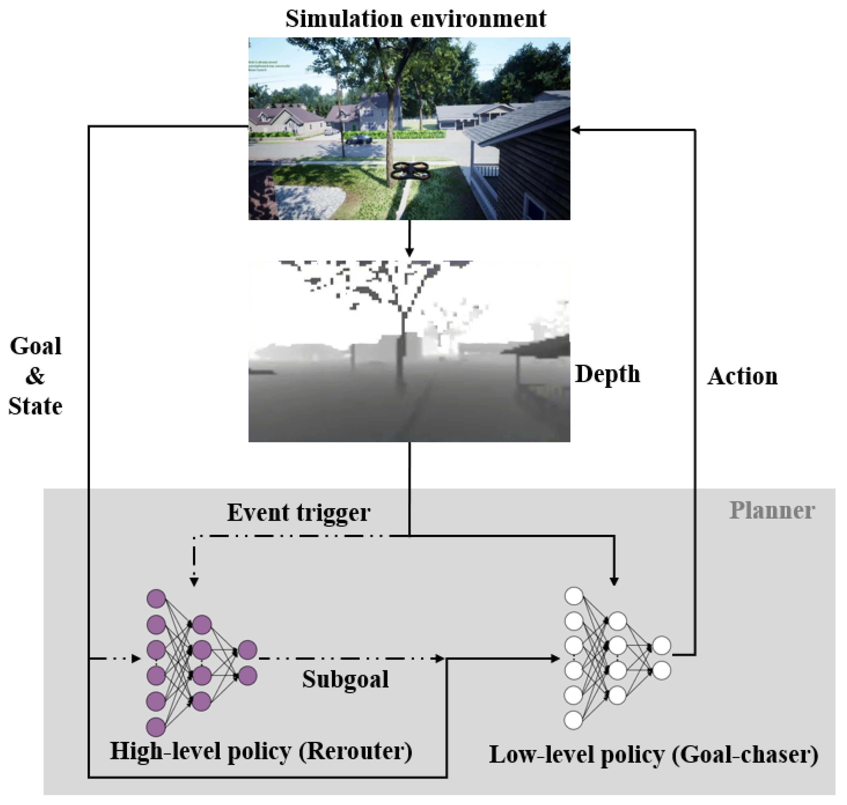
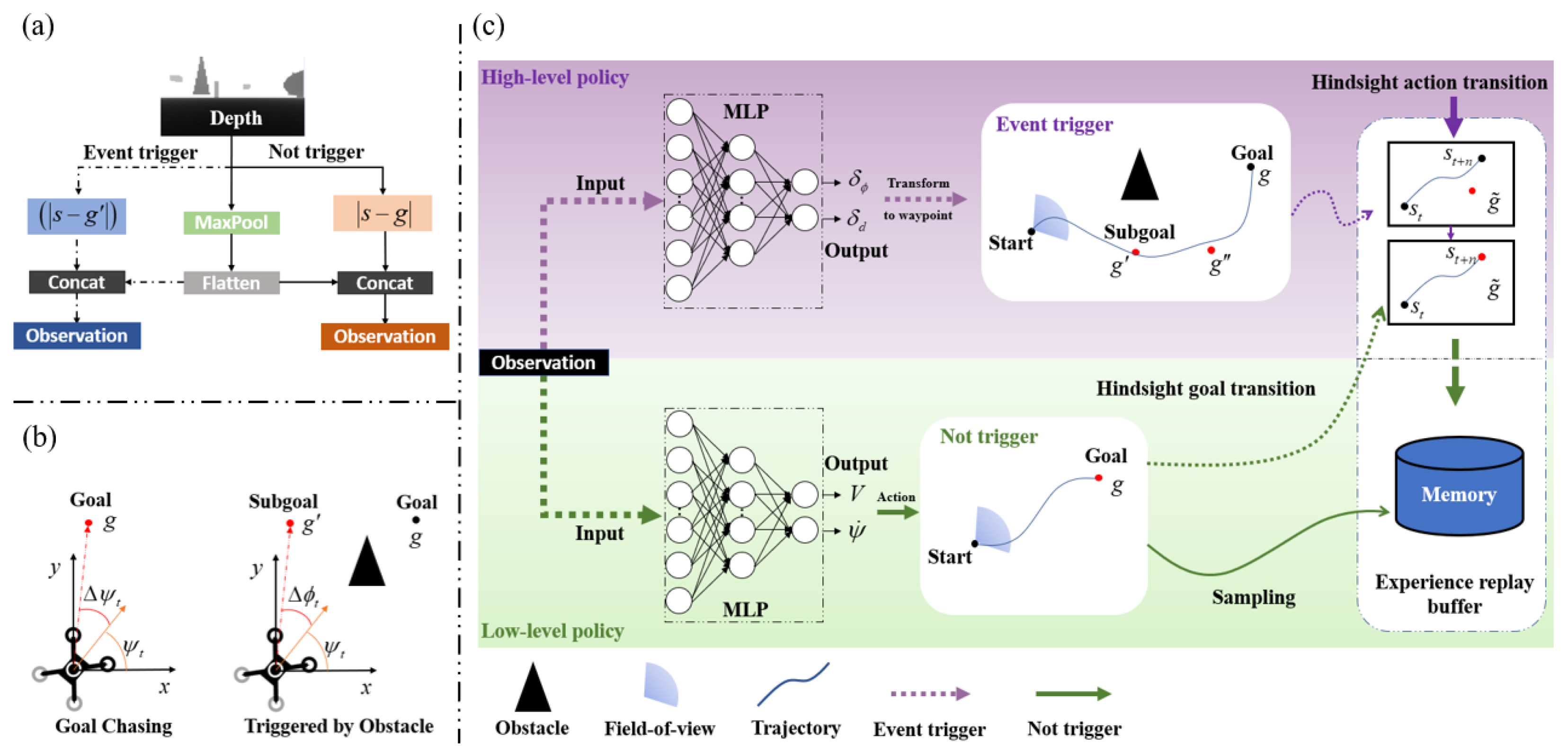
3. Event-Triggered Bi-Level Hierarchical Planner (ETHP)

For UAV autonomous navigation in unknown environments, the planner not only needs to approach the target point but also needs to avoid obstacles that suddenly occur in the field of view. Although an efficient framework for partially unknown environments [27] has been proposed, most of the common outdoor task scenarios such as rescue and resource exploration need to face a fully unknown environment.

Existing methods employ a single high-capacity DNN to deal with this challenge, which lacks explainability and has poor generalization ability. In contrast, we propose a novel event-triggered bi-level hierarchical planner (ETHP), where each level has a physically meaningful optimization goal. The hierarchical structure allows both levels to use a lightweight MLP (multilayer perceptron) network that contains only three layers of $(64,32,2)$ number of neurons, respectively, which significantly improves training efficiency.

Moreover, as shown in Figure 2b,c, we design the “event-trigger” rule, which plans the collision avoidance path reactively. The high-level policy will be triggered to generate intermediate waypoints only if obstacles appear in the field of view (we set the trigger distance, $\beta$). The low-level policy tracks these subgoals in sequence to avoid obstacles. Otherwise, the low-level policy will keep tracking the goal point. The “event-trigger” rule improves the collision avoidance training efficiency and success rate by reducing the chance of generating wrong subgoals. The whole pipeline of ETHP (Algorithm 1) is described as follows:

Algorithm 1: ETHP

3.1. The Low-Level Policy (Goal Chaser)

We consider the two-dimensional navigation task and choose the linear velocity and yaw rate $(V,\dot{\psi })$ as the output of the low-level policy, that is, the control command to the UAV. We name the low-level policy goal-chaser, because it is trained to chase either the goal point or the subgoal point generated by the high-level policy. Its policy network is denoted by $\mu (O;\theta )$, where O is the input to the policy network and $\theta$ are the parameters of the network. We refer to O as the observation, which is constructed by the concatenation of the (max-pooled) depth image and the distance to the (sub)goal (See Figure 2a). Specifically, we have

$$O=\left\{\begin{array}{cc} (depth,∥s-g∥),\hfill & \mathrm{no}\mathrm{obstacle}\hfill \\ (depth,∥s-g^{\prime }∥),\hfill & \mathrm{triggered}\mathrm{by}\mathrm{obstacle},\hfill \end{array}\right.$$

(6)

where state $s=(x_t,y_t,{\psi }_t,V_t)$ contains the current position $(x_t,y_t)$, yaw angle, ${\psi }_t$, and velocity, $V_t$, of the UAV, respectively. For convenience, we slightly abuse the notation to denote the 2D Euclidean distance between the UAV and the (sub)goal by $∥s-g∥$ ($∥s-g^{\prime }∥$). To distinguish the triggered and non-triggered cases better, we use $\Delta {\psi }_t$ and $\Delta {\varphi }_t$ to describe the relative yaw angles with respect to the goal and subgoal, separately; see Figure 2b for the illustration. The goal-chaser will know the distance and the size of obstacles from the depth image. Based on the above input, the goal-chaser will determine when to reduce the speed and whether to adjust the yaw angle in advance.

When in the triggered case, the high-level policy is designed to generate subgoals that are always in the field-of-view of the depth camera. Such a constraint reduces not only the action space of the rerouter but also the state space of the goal-chaser, which improves the sampling efficiency significantly. The reward function for the goal-chaser is divided into a sparse part and a dense part, as follows:

$$r_t^{\mathrm{low}}=r_{\mathrm{sparse}}+r_{\mathrm{dense}},$$

(7)

where

$$r_{\mathrm{sparse}}=\left\{\begin{array}{cc}{R}_{\mathrm{reach}},\hfill & \mathrm{if}\mathrm{goal}\mathrm{is}\mathrm{reached}\hfill \\ R_{\mathrm{warn}},\hfill & \mathrm{if}\mathrm{rerouter}\mathrm{is}\mathrm{triggerred}\hfill \\ 0,\hfill & \mathrm{else}\hfill \end{array}\right.$$

(8)

and

$$r_{\mathrm{dense}}=k_1\ast (d_{t-1}-d_t)-k_2\ast \Delta ,$$

(9)

where $\Delta =\Delta {\psi }_t$ or $\Delta {\varphi }_t$ is the relative yaw angle between the quadrotor and the (sub)goal. The dense reward is used to incentivize the goal-chaser to reach the goal as fast as possible and keep heading toward the (sub)goal. In the training, we choose $R_{\mathrm{reach}}=10.0$, $R_{\mathrm{warn}}=-5.0$, $k_1$, $k_1=1.5$, and $k_2=0.5$.

3.2. The High-Level Policy (Rerouter)

As shown in Figure 2c, the high-level policy is a reactive collision avoidance rerouter that is triggered by the clearance distance. We set the trigger distance $\beta =5$ m during our training. The action space of the rerouter consists of the search angle (the range of angles in which subgoal is generated) and the forward distance $({\delta }_{\varphi },{\delta }_d)$ of the subgoal point. Since the maximum distance of the depth image is 20 m, and the field-of-view of the depth camera is $90{}^{°}$ in our simulation environment, we define a field-of-view constraint for these two actions as ${\delta }_{\varphi }\in (-30{}^{°},30{}^{°})$ and ${\delta }_d\in$ (0.5 m, 8 m). This is to make sure that the subgoal generated by the rerouter is safe. Meanwhile, the size of the action space of the rerouter is therefore reduced, which improves the training efficiency. The action of the rerouter is transformed to a waypoint in the world frame easily as follows:

$$\begin{array}{cc}\hfill x_g& =x+cos({\delta }_{\varphi }+\psi )·{\delta }_{\varphi }\hfill \\ \hfill y_g& =y+sin({\delta }_{\varphi }+\psi )·{\delta }_d\hfill \end{array}$$

(10)

The input of the rerouter also contains the state and depth image. The rerouter generates the waypoint mainly based on the distance and size of obstacles. The rerouter is trained to react to obstacles based on the following reward function:

$$r_t^{\mathrm{high}}=\left\{\begin{array}{cc}{R}_{\mathrm{crash}},\hfill & \mathrm{if}\mathrm{crash}\hfill \\ k_3\ast (d_t^{obs}-d_{t-1}^{obs}),\hfill & \mathrm{otherwise}\hfill \end{array}\right.$$

(11)

where $d_t^{obs}$ is the distance between the UAV and obstacles at time t. In the training, we set $R_{\mathrm{crash}}=-20.0$ and $k_3=2.5$.

3.3. Hindsight Transitions for Bi-Level Hierarchical Planner

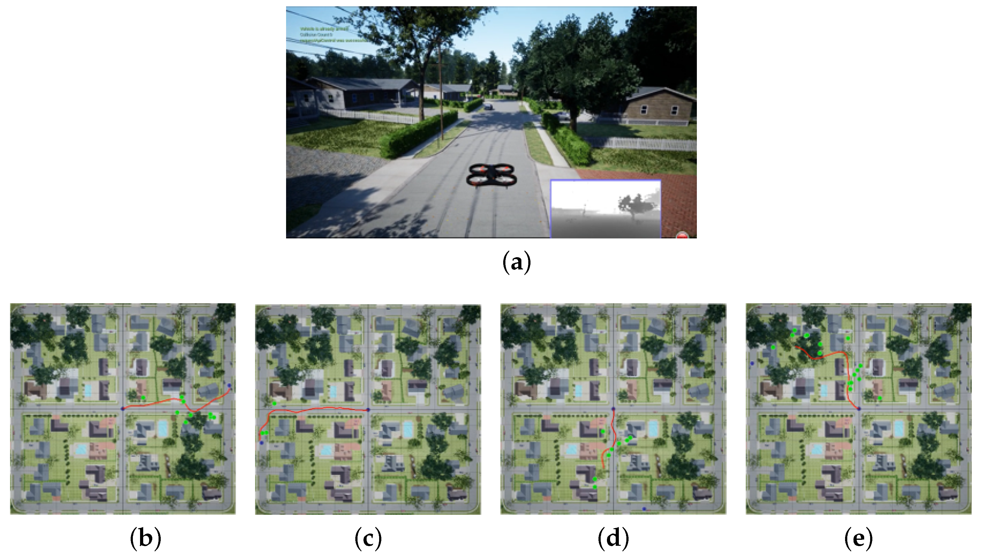
Inspired by HAC [12], in order to avoid the non-stationary problem for the high-level policy training, we supplement the experience replay buffer of the high-level policy with the hindsight action transitions. As shown on the right of Figure 2c, in the triggered case, if the current position $(x_{t+n},y_{t+n})$ is within the field-of-view, we will collect the experience with hindsight action transitions at each timestep $t+n$ after the high-level policy is triggered at timestep t. Specifically, we collect the following tuple for the high-level policy:

$$\begin{array}{c}\hfill [O_t=(depth,x_t,y_t,V_t,\Delta {\varphi }_t),a=F(O_t,O_{t+n}),r=r_t^{\mathrm{high}},\\ \hfill O_{t+1}=(depth,x_{t+n},y_{t+n},V_t,0),g=(x,y)]\end{array}$$

(12)

where the action a for the high-level policy is calculated by the current position $(x_{t+n},y_{t+n})$ and the last position $(x_t,y_t)$ where the high-level policy is triggered:

$$F(O_t,O_{t+n})=({\delta }_{{\varphi }_t},{\delta }_{d_t})$$

(13)

and:

$${\delta }_{{\varphi }_t}=arctan\frac{y_{t+n}-y_t}{x_{t+n}-x_t}$$

(14)

$${\delta }_{d_t}=\sqrt{{(x_{t+n}-x_t)}^2+{(y_{t+n}-y_t)}^2}$$

(15)

We also supplement the low-level policy with hindsight goal transitions, which substantially improves the proportion of good samples. The tuple of our hindsight action transition for low-level policy can be described as follows:

$$\begin{array}{c}\hfill [O_t=(depth,x_t,y_t,V_t,\Delta {\varphi }_t),a=(V_t,\dot{{\psi }_t}),r=R_{\mathrm{reach}},\\ \hfill O_{t+1}=(depth,x_{t+1},y_{t+1},V_t,\Delta {\varphi }_{t+1}),\tilde{g}=(x_{t+1},y_{t+1})]\end{array}$$

(16)

where $\tilde{g}$ is the actual position achieved by the agent (ideal subgoal). We will demonstrate in the next section that the hindsight transitions significantly increase the training efficiency for both levels of policies.

4. Experiment

We train our algorithm in a simulation environment built upon the Microsoft Airsim simulator [28]. It is shipped with high-fidelity quadrotor models and offers a proportional–integral flight controller. To evaluate the merits of the proposed planner better, we also train several other baseline planners using HAC, TD3, SAC, PPO, and DDPG, respectively. These planners share the same network structure and inputs as those in ETHP. The reward function for the baseline planners and each level of HAC planner is the same. The reward function for these planners contains the main items from ETHP reward function:

$${\tilde{r}}_t=\left\{\begin{array}{cc}{R}_{\mathrm{reach}},\hfill & \mathrm{if}\mathrm{goal}\mathrm{reach}\hfill \\ R_{\mathrm{crash}},\hfill & \mathrm{if}\mathrm{crash}\hfill \\ {\tilde{r}}_{dense},\hfill & \mathrm{otherwise}\hfill \end{array}\right.$$

(17)

where:

$${\tilde{r}}_{dense}=k_3\ast (d_t^{obs}-d_{t-1}^{obs})+k_1\ast (d_{t-1}-d_t)-k_2\ast \Delta \psi$$

(18)

with all the coefficients and hyperparameters the same as ETHP. For the training, the learning rate is set as ${10}^{-4}$ for all the policies.

As shown in Figure 3, the training simulation environment is a square area with a side length of 80 m. There are four types of obstacles randomly distributed in the training environment, with all cuboids suspended in the air, and each type of geometry is of different widths and heights. The evaluation environment in Figure 4 is a more complex photorealistic residential area with a side length of 140 m, and there are different sizes of trees, houses, and wire poles concentrated on both sides of the roads. For both training and evaluation environments, the start point of the UAV is fixed at the center of the environment, and the goal point is randomly sampled at a distance of 70 m or 90 m from the start point.

To evaluate the effectiveness of our algorithm better, we test our algorithm in another simulation environment that is different from the training one. As shown in Figure 4, the simulation environment used for testing contains houses and trees, obstacles that have never appeared in the training environment. In addition, as shown in Figure 5, we also deploy our algorithm on a quadrotor and test the performance of our algorithm in a real environment. In the following sections, we will detail the performance of our algorithm in the above environments.

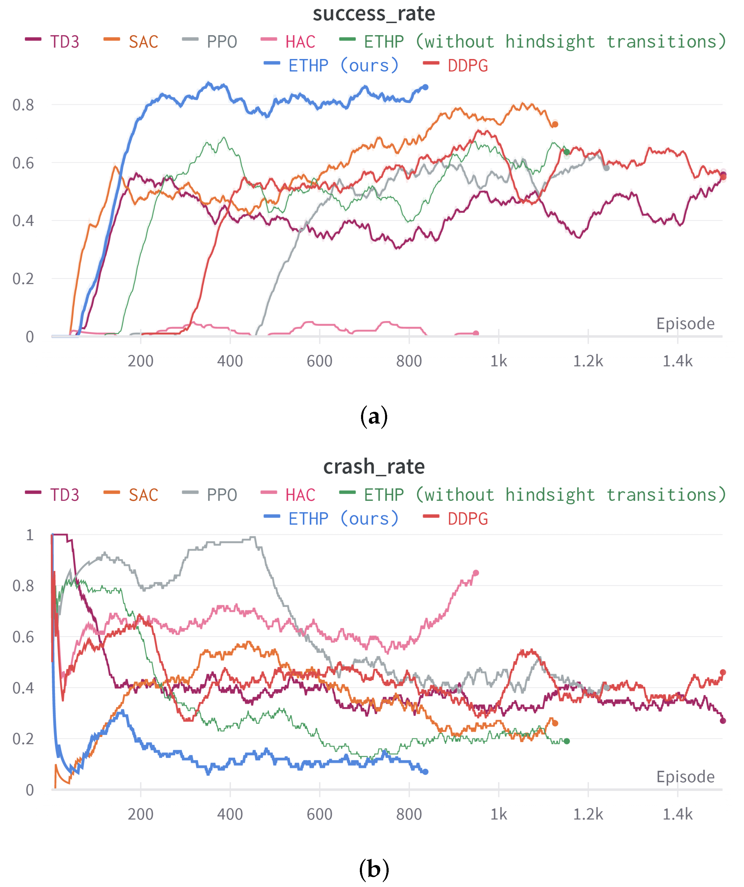
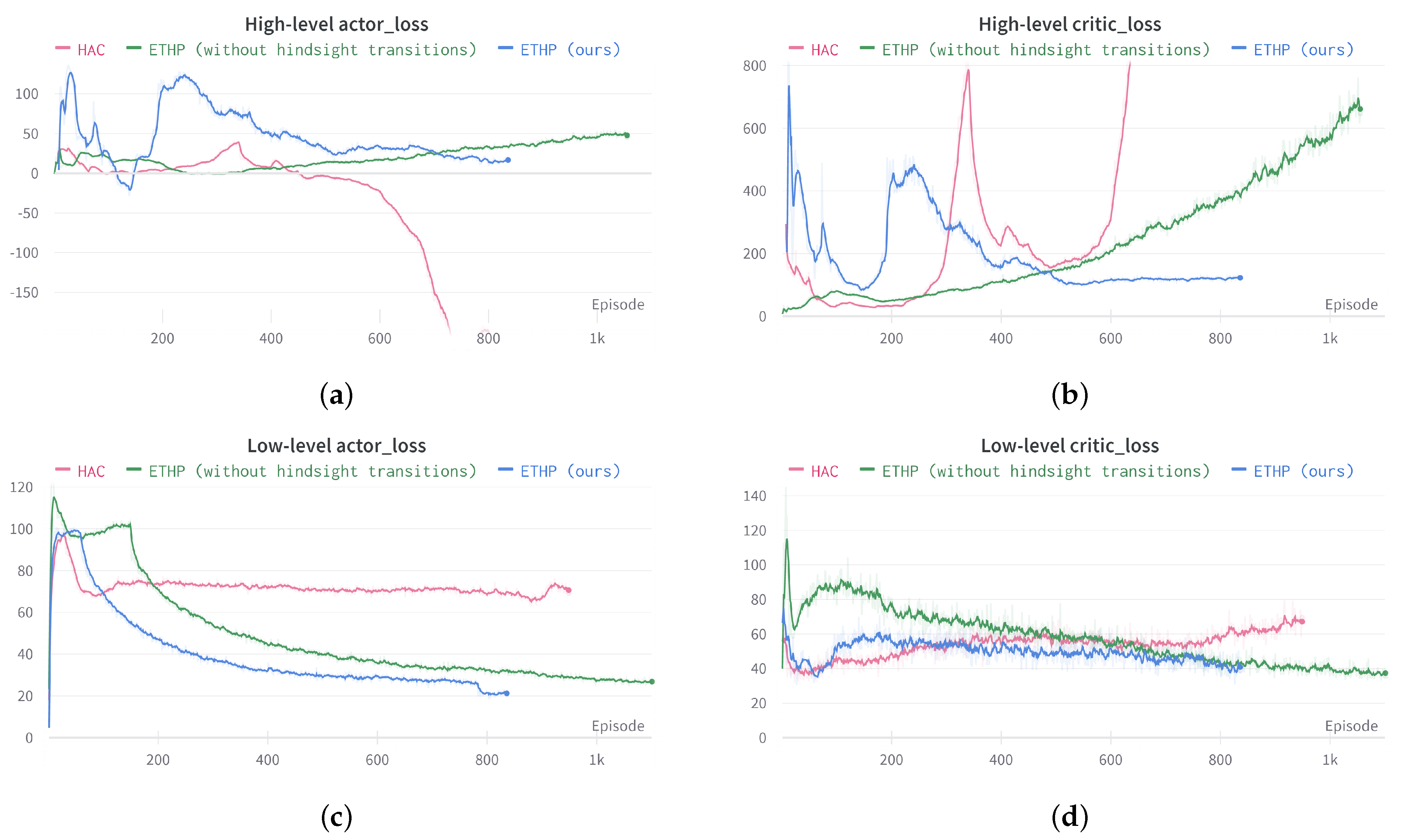
4.1. Comparison Experiment

We compare the performances of ETHP, ETHP (without hindsight transitions), and the other baseline planners in the training environment, shown in Figure 6. The proposed algorithm ETHP achieves the best performance. We record the performance of the final trained models of the different algorithms in

Table 1. Comparison of different algorithms (Dates in bold are the performance of ETHP).

Algorithms	Success Rate	Crash Rate
ETHP (ours)	91%	5%
ETHP (wht)	62%	19%
SAC	73%	24%
PPO	58%	39%
TD3	56%	28%
DDPG	53%	47%
HAC	3%	88%

, which shows that the ETHP achieves the highest success rate of about $90\%$ and the lowest crash rate of about $5\%$. These rates indicate that ETHP has the best tracking performance and collision avoidance performance, respectively. In contrast, the baseline planners have lower success rates and higher crash rates. SAC has the best performance among the baseline planners. Due to the stochastic exploration policy, SAC converges faster than all the other planners. However, it seems difficult for SAC to achieve its best performance quickly, as the stochastic policy will interfere with its evolutionary direction. Meanwhile, by comparing the performance of ETHP with that of ETHP (without hindsight transitions), we found that, as the low-level policy achieves fewer good samples, the success rate decreases significantly. But, even without hindsight transitions, the learning speed and performance of our bi-level hierarchical planner is still better than the baseline DDPG.

From Figure 7 we can see that the HAC planner achieves the result of failure training, as its high-level policy’s actor and critic loss is divergence. This is mainly due to both two levels of policies of HAC using the same reward function. Although there are many chances for the low-level policy to achieve $R_{\mathrm{reach}}$ when it reaches the subgoal and starts a virtuous cycle, the high-level policy somehow has few chances to achieve ‘good’ samples and is easily stuck into the collision conditions since the low-level policy will quickly learn to fly around the obstacles so that it can achieve more rewards. This result shows that it is hard for the basic hierarchical reinforcement learning algorithm to succeed in this task.

To evaluate the contribution of hindsight transitions in more detail, we compare the training losses of the two levels of policies. Figure 7c,d show that, with hindsight goal transitions, the convergence of the low-level policy is significantly faster. The impact of hindsight action transitions on the high-level policy is much more pronounced than hindsight goal transitions on the low-level policy. As can be seen in Figure 7a,b, if there are no supplies of hindsight action transitions for the high-level policy, the training does not even converge for both actor and critic networks.

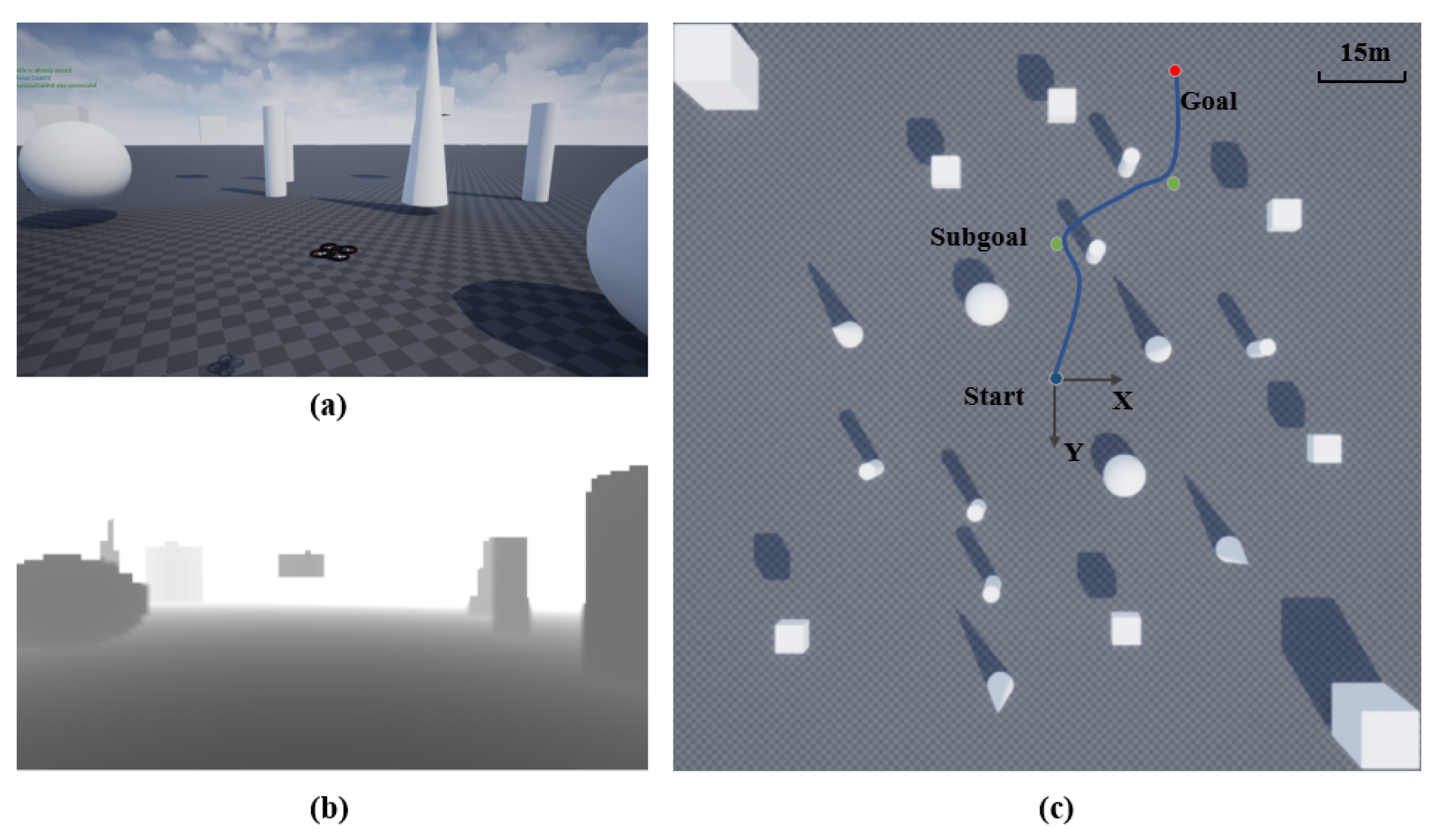
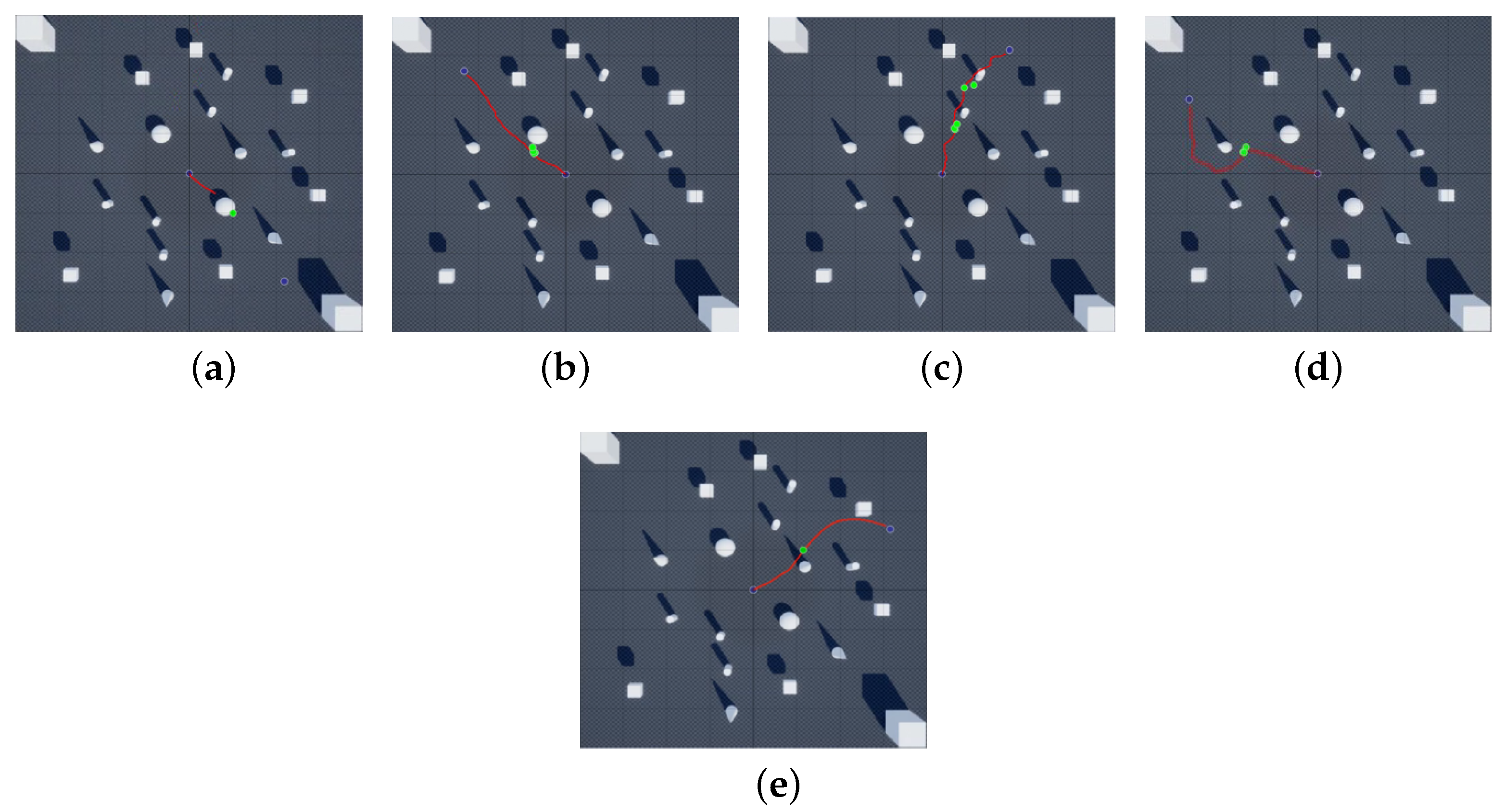
4.2. Evaluation Experiments

We evaluate ETHP in both training and evaluation environments. The performance of ETHP in different training stages of the training environment is shown in Figure 8. We can see from Figure 8a that, in the initial stage of training, the trajectory is almost directly towards the goal, but the high-level policy in this stage cannot react to obstacles properly. It also indicates that the low-level policy learns much faster than the high-level policy. From Figure 8b, we can see that the high-level policy starts to generate waypoints for avoiding collisions, but these waypoints are not good as they are too close to the obstacle. In Figure 8c,d, new changes happen with the low-level policy, and it starts to ignore some of the wrong waypoints generated from the high-level policy. Meanwhile, from these two stages, we can see that the high-level policy’s ability to generate safe waypoints is improving. At last, from Figure 8e, the low-level policy can follow the waypoints generated by the high-level policy very well, and the subgoal generated by the high-level policy can avoid the obstacle very well.

We record the dynamic state of the UAV in a random evaluation experiment under the policy trained after 700 episodes (referred to as $Mode{l}_{700}$ in the sequel) to analyze the potential of ETHP in optimizing the path both spatially and temporally. As shown in Figure 9, we can divide the whole flight into three typical stages. In stage one, since the maximum distance of the depth image is 20 m, we can see that the yaw angles change dramatically at first, which indicates that the planner is in the triggered mode to avoid obstacles. The goal-chaser needs to adjust the yaw rate quickly to track the subgoals generated by the high-level policy. At the same time, the velocity is commanded to decrease monotonically for trajectory tracking accuracy. In stage two, we see that the change of yaw angle is decreasing, but the velocity is becoming bigger, which indicates that the UAV has passed the area with obstacles, so it accelerates to approach the target. As for the last stage shown in the green area, when the UAV is close to the target point, the planner starts to reduce the speed and adjust the yaw carefully to reach the target accurately.

To test the generalization ability of the trained ETHP further, the model learned in the simple training environment is tested in the photorealistic evaluation environment without any tuning (see Figure 4). This evaluation environment is much larger than the training environment. It contains a large number of objects with various shapes, such as branches, leaves, and thin poles in the environment. These cause collision avoidance to be even more challenging. As can be seen from Figure 4b,c, the proposed ETHP can still complete the task in these unseen environments. However, in cases where there are too many trees or poles in the surrounding areas of the target, such as (d) and (e), the high-level policy failed to generate rerouting waypoints to successfully reach the goal point. More training in a variety of different types of environments is needed to further improve collision avoidance performance.

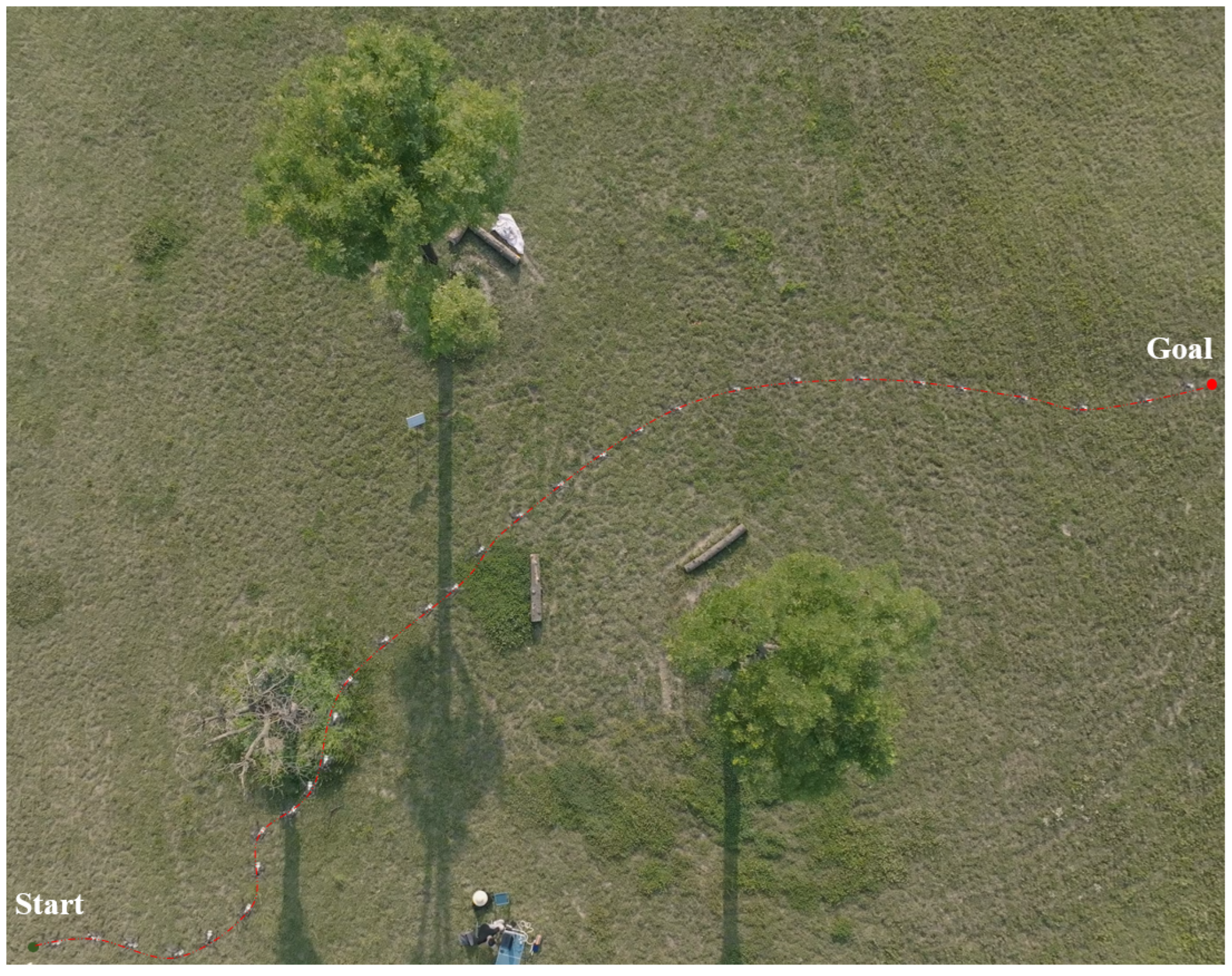
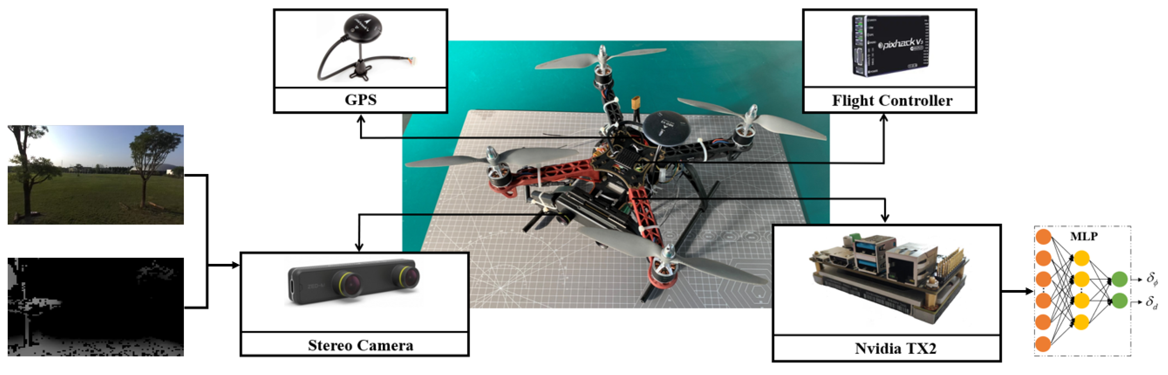
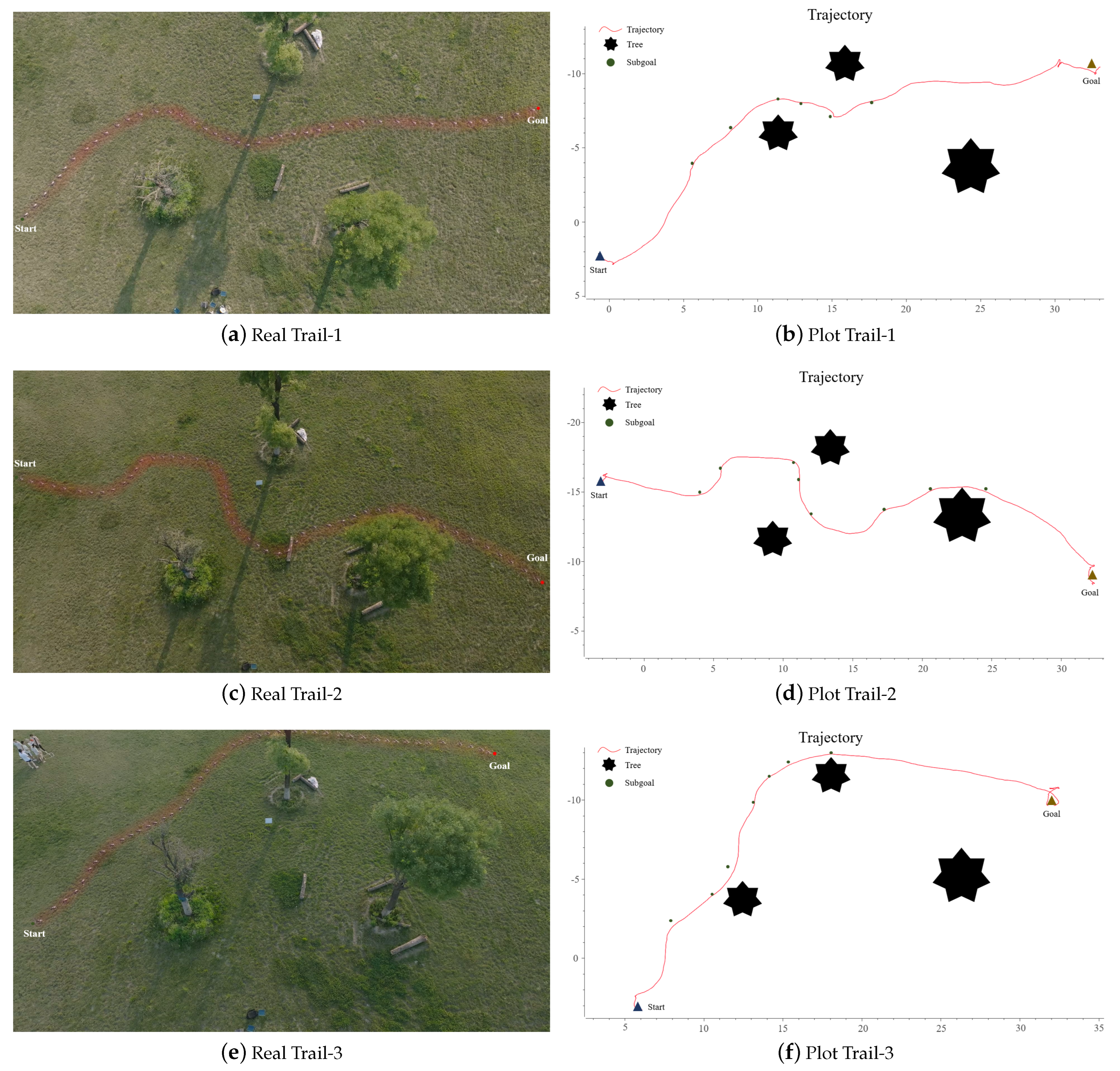
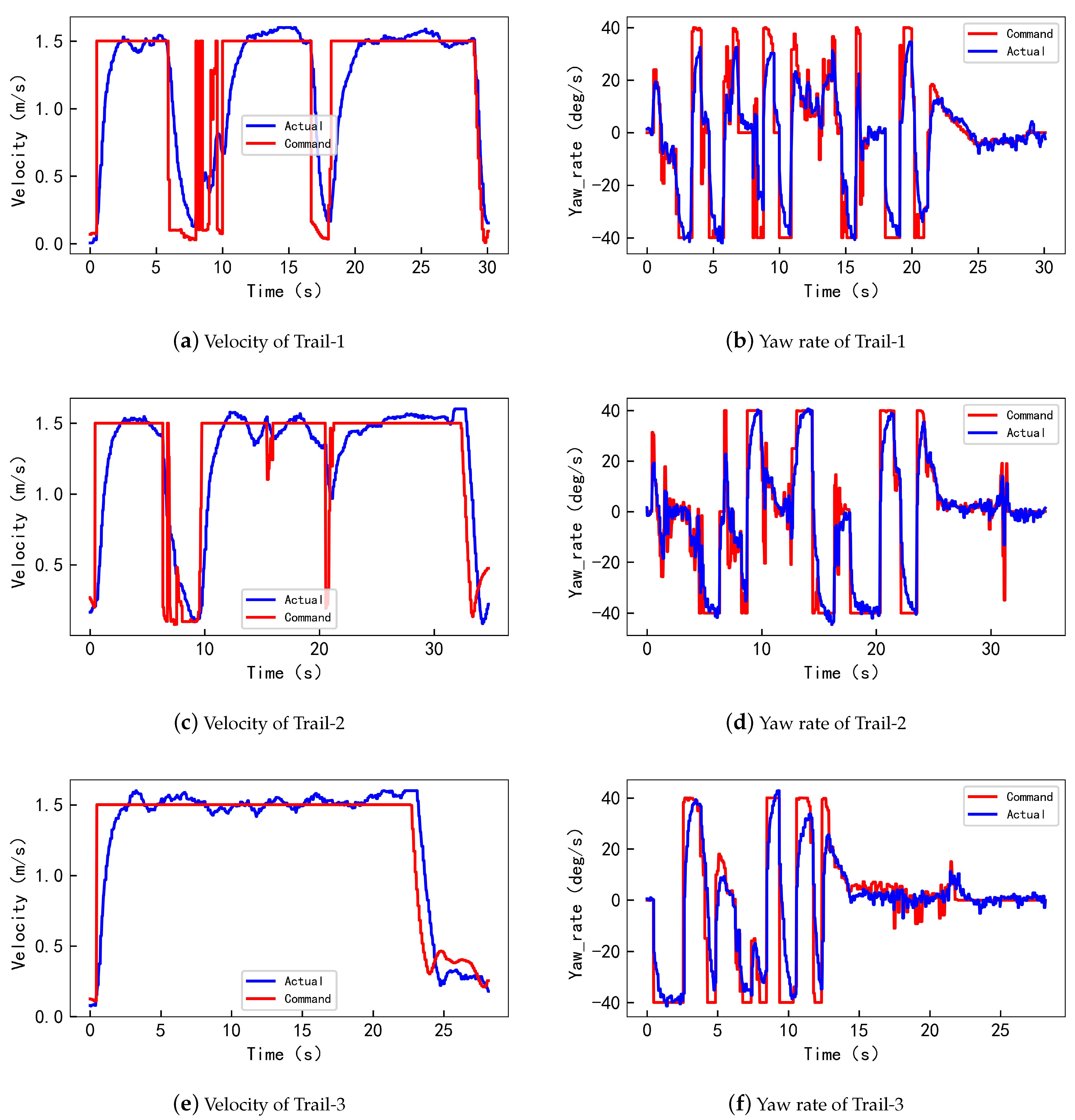
4.3. Real Flight Test

We deploy our algorithm on a quadrotor and test the effect of flying in a real environment. As shown in Figure 10, the drone is equipped with a Pixhawk flight controller, a GPS, an Nvidia TX2 on-board calculator, and a ZED Mini stereo camera. The stereo camera continuously provides reliable depth images of the front environment, while the GPS and Pixhawk provide the location and attitude of the drone. Meanwhile, the onboard computer is running the ETHP and takes the above information as inputs and outputs the velocity and yaw rate to Pixhawk.

In order to ensure the safety of experimental equipment and personnel, we map the velocity range of (0, 5 m/s) to (0, 1.5 m/s). Meanwhile, the maximum range of yaw rate is mapped from $(-{60}^{°},{60}^{°})$ to $(-{40}^{°},{40}^{°})$. To implement the above mapping, the output of the network is multiplied by a scaling matrix $[\frac{3}{10},\frac{2}{3}]$.

We set the UAV to start from different locations and finally reach different goals. As shown in Figure 11, the UAV successfully reaches the goals in each test, and, in the time-lapse photography, we can see that the flight trajectories are smooth and reasonable.

To show more details, we record the speed, position, and attitude data with the Pixhawk Flight Log. We then plot these data with the outputs of the high-level policy recorded by the onboard computer into Figure 11. As shown in Figure 11b,d,f, the high-level policy plays an important role when the UAV approaches obstacles. From the plotted trajectories, we can see that, whenever an obstacle appears forward, the high-level policy will be triggered and output a subgoal, which causes the lower-level policy to chase these subgoals, and ultimately the UAV will fly out a beautiful turning curve to avoid all the obstacles.

As shown in Figure 12, by plotting the changes of speed and yaw rate throughout the whole flight mission, we can see the characteristics of the low-level policy and the impact of the high-level policy more clearly. Due to the low-level policy being motivated by shortening the distance between the current position to the goal, through the velocity change curves in Figure 12a,c,e, it always trying to find the fastest way and output the maximum speed to reach the goals. But, when obstacles occur, as the high-level policy sends the low-level policy a new goal (which is the subgoal), the low-level policy will decrease the velocity and chase the subgoal. Figure 12b,d,f also show that, when avoiding the obstacles, the yaw rate changes frequently. But, when there is no obstacle in front, as no subgoal will be sent to the low-level policy, the yaw rate will not have any big change and the velocity will always keep the biggest value to reaching the final goal.

The real flight tests show that our method has consistent performance in both simulation environments and unknown real environments. The above results prove that our method has strong generalization ability and engineering application value.

5. Conclusions

In this work, we propose an event-triggered bi-level hierarchical planner (ETHP) for UAV autonomous navigation in unknown environments. Compared with the traditional end-to-end DNN-based motion planners, our method exploits the bi-level optimization nature of the navigation task to achieve highly efficient training and better optimality. In addition, the bi-level structure provides additional training flexibility and efficiency, as it allows the reuse of the data for training both policies despite their different objectives. The rules developed for hindsight transitions significantly improve training efficiency. We compared ETHP with several DNN-based baseline planners, and ETHP achieved the highest success rate and lowest crash rate. The evaluation experiments in unseen environments show that ETHP generalizes well and has great potential in spatio–temporal path optimization. However, since the location of the UAV needs to be provided by GPS, the application of our method in indoor environments is limited. In future research, we will try to solve this problem so that our method has more application scenarios.

References

1. Tomic, T.; Schmid, K.; Lutz, P.; Domel, A.; Kassecker, M.; Mair, E.; Grixa, I.L.; Ruess, F.; Suppa, M.; Burschka, D. Toward a fully autonomous UAV: Research platform for indoor and outdoor urban search and rescue. IEEE Robot. Autom. Mag. 2012, 19, 46–56. [Google Scholar] [CrossRef]
2. Özaslan, T.; Loianno, G.; Keller, J.; Taylor, C.J.; Kumar, V.; Wozencraft, J.M.; Hood, T. Autonomous navigation and mapping for inspection of penstocks and tunnels with MAVs. IEEE Robot. Autom. Lett. 2017, 2, 1740–1747. [Google Scholar] [CrossRef]
3. Loianno, G.; Spurny, V.; Thomas, J.; Baca, T.; Thakur, D.; Hert, D.; Penicka, R.; Krajnik, T.; Zhou, A.; Cho, A.; et al. Localization, grasping, and transportation of magnetic objects by a team of mavs in challenging desert-like environments. IEEE Robot. Autom. Lett. 2018, 3, 1576–1583. [Google Scholar] [CrossRef]
4. Liu, X.; Chen, S.W.; Nardari, G.V.; Qu, C.; Ojeda, F.C.; Taylor, C.J.; Kumar, V. Challenges and Opportunities for Autonomous Micro-UAVs in Precision Agriculture. IEEE Micro 2022, 42, 61–68. [Google Scholar] [CrossRef]
5. Ma, Z.; Wang, Z.; Ma, A.; Liu, Y.; Niu, Y. A Low-Altitude Obstacle Avoidance Method for UAVs Based on Polyhedral Flight Corridor. Drones 2023, 7, 588. [Google Scholar] [CrossRef]
6. Zhao, S.; Zhu, J.; Bao, W.; Li, X.; Sun, H. A Multi-Constraint Guidance and Maneuvering Penetration Strategy via Meta Deep Reinforcement Learning. Drones 2023, 7, 626. [Google Scholar] [CrossRef]
7. Wang, W.; Zhang, G.; Da, Q.; Lu, D.; Zhao, Y.; Li, S.; Lang, D. Multiple Unmanned Aerial Vehicle Autonomous Path Planning Algorithm Based on Whale-Inspired Deep Q-Network. Drones 2023, 7, 572. [Google Scholar] [CrossRef]
8. Loquercio, A.; Kaufmann, E.; Ranftl, R.; Müller, M.; Koltun, V.; Scaramuzza, D. Learning high-speed flight in the wild. Sci. Robot. 2021, 6, eabg5810. [Google Scholar] [CrossRef] [PubMed]
9. He, L.; Aouf, N.; Whidborne, J.F.; Song, B. Integrated moment-based LGMD and deep reinforcement learning for UAV obstacle avoidance. In Proceedings of the 2020 IEEE International Conference on Robotics and Automation (ICRA), Paris, France, 31 May–31 August 2020; IEEE: Piscataway, NJ, USA, 2020; pp. 7491–7497. [Google Scholar]
10. Pham, H.X.; La, H.M.; Feil-Seifer, D.; Nguyen, L.V. Autonomous uav navigation using reinforcement learning. arXiv 2018, arXiv:1801.05086. [Google Scholar]
11. Loquercio, A.; Maqueda, A.I.; Del-Blanco, C.R.; Scaramuzza, D. Dronet: Learning to fly by driving. IEEE Robot. Autom. Lett. 2018, 3, 1088–1095. [Google Scholar] [CrossRef]
12. Nachum, O.; Gu, S.S.; Lee, H.; Levine, S. Data-efficient hierarchical reinforcement learning. In Proceedings of the Advances in Neural Information Processing Systems, Montreal, QC, Canada, 3–8 December 2018; Volume 31. [Google Scholar]
13. Andrychowicz, M.; Wolski, F.; Ray, A.; Schneider, J.; Fong, R.; Welinder, P.; McGrew, B.; Tobin, J.; Pieter Abbeel, O.; Zaremba, W. Hindsight experience replay. In Proceedings of the Advances in Neural Information Processing Systems, Long Beach, CA, USA, 4–9 December 2017; Volume 30. [Google Scholar]
14. Pateria, S.; Subagdja, B.; Tan, A.h.; Quek, C. Hierarchical reinforcement learning: A comprehensive survey. ACM Comput. Surv. 2021, 54, 1–35. [Google Scholar] [CrossRef]
15. Dayan, P.; Daw, N.D. Decision theory, reinforcement learning, and the brain. Cogn. Affect. Behav. Neurosci. 2008, 8, 429–453. [Google Scholar] [CrossRef] [PubMed]
16. Barto, A.G.; Mahadevan, S. Recent advances in hierarchical reinforcement learning. Discret. Event Dyn. Syst. 2003, 13, 41–77. [Google Scholar] [CrossRef]
17. Dayan, P.; Hinton, G.E. Feudal reinforcement learning. In Proceedings of the Advances in Neural Information Processing Systems, San Francisco, CA, USA, 30 November–3 December 1992; Volume 5. [Google Scholar]
18. Sutton, R.S.; Precup, D.; Singh, S. Between MDPs and semi-MDPs: A framework for temporal abstraction in reinforcement learning. Artif. Intell. 1999, 112, 181–211. [Google Scholar] [CrossRef]
19. Sun, P.; Sun, X.; Han, L.; Xiong, J.; Wang, Q.; Li, B.; Zheng, Y.; Liu, J.; Liu, Y.; Liu, H.; et al. Tstarbots: Defeating the cheating level builtin ai in starcraft ii in the full game. arXiv 2018, arXiv:1809.07193. [Google Scholar]
20. Vezhnevets, A.S.; Osindero, S.; Schaul, T.; Heess, N.; Jaderberg, M.; Silver, D.; Kavukcuoglu, K. Feudal networks for hierarchical reinforcement learning. In Proceedings of the International Conference on Machine Learning, PMLR, Sydney, Australia, 6–11 August 2017; pp. 3540–3549. [Google Scholar]
21. Levy, A.; Konidaris, G.; Platt, R.; Saenko, K. Learning multi-level hierarchies with hindsight. arXiv 2017, arXiv:1712.00948. [Google Scholar]
22. Schaul, T.; Horgan, D.; Gregor, K.; Silver, D. Universal value function approximators. In Proceedings of the International Conference on Machine Learning, PMLR, Lille, France, 7–9 July 2015; pp. 1312–1320. [Google Scholar]
23. Kulkarni, T.D.; Narasimhan, K.; Saeedi, A.; Tenenbaum, J. Hierarchical deep reinforcement learning: Integrating temporal abstraction and intrinsic motivation. In Proceedings of the Advances in Neural Information Processing Systems, Barcelona, Spain, 5–10 December 2016; Volume 29. [Google Scholar]
24. Silver, D.; Lever, G.; Heess, N.; Degris, T.; Wierstra, D.; Riedmiller, M. Deterministic policy gradient algorithms. In Proceedings of the International Conference on Machine Learning, PMLR, Beijing, China, 22–24 June 2014; pp. 387–395. [Google Scholar]
25. Peters, J.; Schaal, S. Natural actor-critic. Neurocomputing 2008, 71, 1180–1190. [Google Scholar] [CrossRef]
26. Tedrake, R.; Zhang, T.W.; Seung, H.S. Stochastic policy gradient reinforcement learning on a simple 3D biped. In Proceedings of the 2004 IEEE/RSJ International Conference on Intelligent Robots and Systems (IROS) (IEEE Cat. No. 04CH37566), Sendai, Japan, 28 September–2 October 2004; IEEE: Piscataway, NJ, USA, 2004; Volume 3, pp. 2849–2854. [Google Scholar]
27. Mugnai, M.; Teppati Losé, M.; Herrera-Alarcón, E.P.; Baris, G.; Satler, M.; Avizzano, C.A. An Efficient Framework for Autonomous UAV Missions in Partially-Unknown GNSS-Denied Environments. Drones 2023, 7, 471. [Google Scholar] [CrossRef]
28. Shah, S.; Dey, D.; Lovett, C.; Kapoor, A. Airsim: High-fidelity visual and physical simulation for autonomous vehicles. In Proceedings of the Field and Service Robotics, Zurich, Switzerland, 12–15 September 2017; Springer: Cham, Switzerland, 2018; pp. 621–635. [Google Scholar]
Figure 1. Event-triggered bi-level hierarchical planner (shown in the dashed frame). The planner directly maps from depth images to velocity and heading references. The high-level policy is triggered by the close obstacles and generates rerouting subgoals for collision avoidance. The low-level policy chases the (sub)goal.
Drones 07 00690 g001
Figure 2. (a) Observation is the concatenation of the (max-pooled) depth image and the distance to the (sub)goal point. (b) If there is no obstacle in the depth image, then the high-level policy is not triggered, and the low-level policy chases the goal point (left figure); In the “event trigger” case, the high-level policy generates a collision avoidance subgoal, g , for the low-level policy to track. (c) Overall ETHP framework. Note that g ˜ is the ideal subgoal by performing the hindsight goal transition.
Drones 07 00690 g002
Figure 3. The simulation environment. (a) The simulator. (b) Depth image from the UAV view. (c) Top view of the environment.
Drones 07 00690 g003
Figure 4. The performance of ETHP without tuning in the high-reality evaluation environment (includes different size of trees, houses, and poles). (a) Evaluation environment. (b) Trail 1 (success trajectory). (c) Trail 2 (success trajectory). (d) Trail 3 (crash trajectory). (e) Trail 4 (crash trajectory).
Drones 07 00690 g004
Figure 5. Real flight test environment (the white dots in the picture are the positions of the UAV at different times captured by time-lapse photography, and the red line shows the entire flight trajectory).
Drones 07 00690 g005
Figure 6. The performance of ETHP, ETHP(without hindsight transitions), and the other baseline planners in the training environment. (a) Success rate. (b) Crash rate.
Drones 07 00690 g006
Figure 7. Training curves of ETHP, ETHP(without hindsight transitions), and the baseline HAC planner in the training environment. (a) Actor loss of high-level policy. (b) Critic loss of high-level policy. (c) Actor loss of low-level policy. (d) Critic loss of low-level policy.
Drones 07 00690 g007
Figure 8. Performance of ETHP at different stages of training. The start point is located at the center of each graph, the red line shows the trajectory of the flight, and the goal point (blue dot) is randomly chosen in each episode. (a) 50 episodes. (b) 100 episodes. (c) 150 episodes. (d) 200 episodes. (e) 700 episodes.
Drones 07 00690 g008
Figure 9. Dynamic states of the UAV with M o d e l 700 : (a) shows the change of distance to the target; (b) shows the change in velocity; and (c) shows the change of yaw.
Drones 07 00690 g009
Figure 10. Real flight test platform.
Drones 07 00690 g010
Figure 11. Real flight trajectories. (a,c,e) show the top view and (b,d,f) show the Flight Log plot trajectories of Trail-1, Trail-2, and Trail-3, respectively.
Drones 07 00690 g011
Figure 12. Real flight attitude. (a,c,e) show the change of velocity and (b,d,f) show the change of yaw rate of Trail-1, Trail-2, and Trail-3, respectively.
Drones 07 00690 g012