Condition Monitoring of the Torque Imbalance in a Dual-Stator Permanent Magnet Synchronous Motor for the Propulsion of a Lightweight Fixed-Wing UAV

Abstract

This paper deals with the development of a model-based technique to monitor the condition of torque imbalances in a dual-stator permanent magnet synchronous motor for UAV full-electric propulsion. Due to imperfections, degradations or uncertainties, the torque split between power lines can deviate from the design, causing internal force-fighting and reduced efficiency. This study demonstrates that, by only elaborating the measurements of speed and direct/quadrature currents of the stators during motor acceleration/deceleration, online estimations of demagnetization and electrical angle misalignment can be obtained, thus permitting the evaluation of the imbalance and total torque of the system. A relevant outcome is that the technique can be used for developing both signal-based and model-based monitoring schemes. Starting from physical first-principles, a nonlinear model of the propulsion system, including demagnetization and electrical angle misalignment, is developed in order to analytically derive the relationships between monitoring inputs (currents and speed) and outputs (degradations). The model is experimentally validated using a system prototype characterized by asymmetrical demagnetization and electrical angle misalignment. Finally, the monitoring effectiveness is assessed by simulating UAV flight manoeuvres with the experimentally validated model: injecting different levels of degradations and evaluating the torque imbalance.

1. Introduction

1.1. Research Context

On the wave of the worldwide goal to decarbonize transport systems, the electrification of propulsion systems nowadays represents one of the most challenging objectives in the design of flying vehicles. With specific reference to long-endurance UAVs, internal combustion engines are expected to be progressively replaced by hybrid electric systems and, eventually, with Full-Electric Propulsion Systems (FEPSs). Electric propulsion would reduce (or eliminate for FEPSs) the CO₂ emissions, abate the noise levels, diminish the thermal signature, and enhance the thrust efficiency and performance of fixed wing UAVs [1,2,3], even if reliability is now an open issue (essentially due to the application novelty) and achievable endurance is much lower than that of UAVs equipped with internal combustion engines (consider that the energy storage of Li-Ion batteries typically reaches about 0.3 MJ/kg, approximately 100 times lower than gasoline data [1]). Within this context, the project TERSA (Tecnologie Elettriche e Radar per Sistemi aeromobili a pilotaggio remoto Autonomi [4,5]) has been funded by the Italian Government together with the Tuscany Regional Government for developing a lightweight full-electric long-endurance UAV (Figure 1 [6]) with the following main characteristics [6]:

• Mass (including payloads): 35 kg;
• Take-off/landing system: pneumatic launcher and parachute/airbags;
• Propulsion system: fixed-pitch twin-blade propeller driven by dual-redundant FEPS (3.5 kW maximum power);
• Relevant payloads: Synthetic Aperture Radar and Sense-And-Avoid System;
• Cruise speed: 26 m/s;
• Flight endurance: 6 h;
• Data-link operational range: 100 km;
• Radar ground swath range: 3 km (0.2 m image reconstruction accuracy).

The project, led by Sky Eye Systems (Italy) in partnership with the University of Pisa and other Italian industries, was successfully completed in December 2022.

1.2. Full-Electric Propulsion Requirements

FEPSs for long-endurance UAVs must be characterized by high compactness, high torque density, high power-to-weight ratio (>6 kW/kg), excellent efficiency (>85%) [2,7,8], and high reliability. For example, the failure rate of a conventional non-redundant electric motor and related electronics typically reaches about three per thousand flight hours [9,10], which is not compliant with the reliability and safety levels required for airworthiness certification [11]. Due to weight and envelope concerns, the use of redundant motors is often unfeasible, so the reliability can be enhanced by unconventional converters or through phase redundancy. Two main solutions are suggested in the literature: one is based on conventional three-leg converters coupled with multiple-phase motors [12,13] or multiple three-phase arrangements [14,15], while the other is based on the use of four-leg converters [10,16,17]. In the second case, the conventional three-leg bridge is equipped with a couple of additional stand-by MOSFETs in order to control the neutral point of the three-phase connection. Though compact and lightweight, the four-leg solution implies a specific design in terms of system hardware (e.g., neutral point accessibility) and software (e.g., drive of additional MOSFETs) [10,18]. Concerning the Permanent Magnet Synchronous Motor (PMSM) architectures, Axial-Flux PMSMs (AFPMSMs) probably represent the best solution in terms of weight, efficiency, adaptability, and torque-to-weight ratio [8], even if their technology readiness is lower than conventional radial-flux PMSMs [19,20].

In pursuing a balance between the above-mentioned considerations, the reference FEPS has been equipped with a dual-stator AFPMSM and two independent electronic control units with a conventional three-leg converter to drive each stator module so that the propulsion system, depending on the mission phase, can operate in active/active or active/stand-by torque-summing configuration.

In a previous work by the authors [5], the diagnosis of electrical and electronic faults of the TERSA FEPS, the design of fault-tolerant control strategies, and the simulation of the failure transients related to the most critical faults have been addressed, but an actual enhancement of the system reliability must also include condition-monitoring activities, aiming to anticipate the occurrence of faults and to support their prognosis (i.e., predictive maintenance). As a relevant example, the thrust output of a dual torque-summing system depends on the sum of electrical torques, so that the effects of a torque imbalance between two stators can remain “hidden” for long time, potentially to the point of causing critical electrical and electronic faults.

1.3. Torque Imbalance between Stator Modules

One of the main issues in the redundant power systems design is the imbalance of torque/force paths. The torque imbalance reduces the system efficiency and increases the electrical loads on one of the two modules, leading to premature degradations and anticipated faults. The torque imbalance can be as follows:

• non-periodic, when related to

  ○

  uniform demagnetization of a module;

  ○

  misalignment of electrical angle due to sensor offset or imperfections of the stator–rotor coupling;

• periodic, when related to

  ○

  different air gap eccentricity;

  ○

  local demagnetization;

  ○

  cogging disturbances;

  ○

  variation of electrical parameters;

  ○

  local damages on mechanical parts and bearings.

Periodic imbalances, accompanied by noise and vibrations, are easier to detect during maintenance or before/after flight, while non-periodic imbalances can remain undetected up to the occurrence of faults.

Demagnetization phenomena are typically due to operation at high temperatures [21] in combination with high current amplitudes along the direct axis, counteracting the permanent magnet field [22]. In particular, the demagnetization can be uniform (producing a reduction in the BEMF amplitude) or local (causing distortions of the BEMF waveform) [23]. High-amplitude direct currents can be related to fault conditions, such as short circuits or open phases [24], but it can also result from the incorrect application of flux-weakening strategies [25]. In aerospace applications, characterized by operation in harsh environments with large temperature variations and load cycles with fast dynamics, irreversible demagnetization is a risk [26]. A wide review on methods for the diagnosis of demagnetization is proposed in [27,28], and most of them are based on flux observers; as relevant examples, Xi [29] and Min [30] apply extended Kalman filtering, Xu et al. [31] implement second-order integral flux observers, Bobtsov et al. [32] apply LTI filters and linear regression, and Uddin [33] develops an adaptive flux estimator. Despite the prediction accuracy, all these methods generally need to elaborate many signals: current signals, voltage signals, angular position, and speed. Furthermore, in most of the cases, a trial-and-error setting procedure of the estimator parameters is required in order to get the best trade-off between filter convergence time and stability due to the intrinsic inaccuracy of the noise covariance matrix model. In this work, a simple and robust approach is proposed, in which the estimation of demagnetization is derived only from measurements of direct/quadrature currents and speed during motor accelerations, and the only parameter to be tuned is the minimum acceleration threshold required for the estimation. In addition, the proposed technique allows us to estimate the electrical angle misalignment, which also impacts the generation of torque imbalance. The technique can be applied as model-based monitoring to single stator PMSMs, or as signal-based monitoring to redundant architectures, even if, in this case, only the asymmetrical behaviours of the modules could be detected.

The paper is organized as follows: Firstly, the reference FEPS model is described starting from physical first-principles, characterizing the effects of demagnetization and electrical angle misalignment on torque output via analytical expressions. Secondly, a model-based monitoring technique is proposed, with the basic objective of estimating system degradations from direct and quadrature current deviations. Successively, an experimental test campaign is defined to characterize the system performances and identify the main model parameters (phase resistance and inductance, speed constants, BEMF waveforms). Finally, the monitoring effectiveness is verified by using the experimentally validated model, also with reference to flight manoeuvre time histories.

2. Materials and Methods

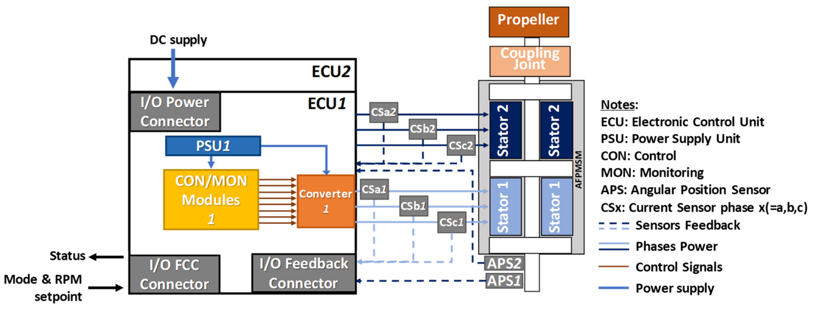
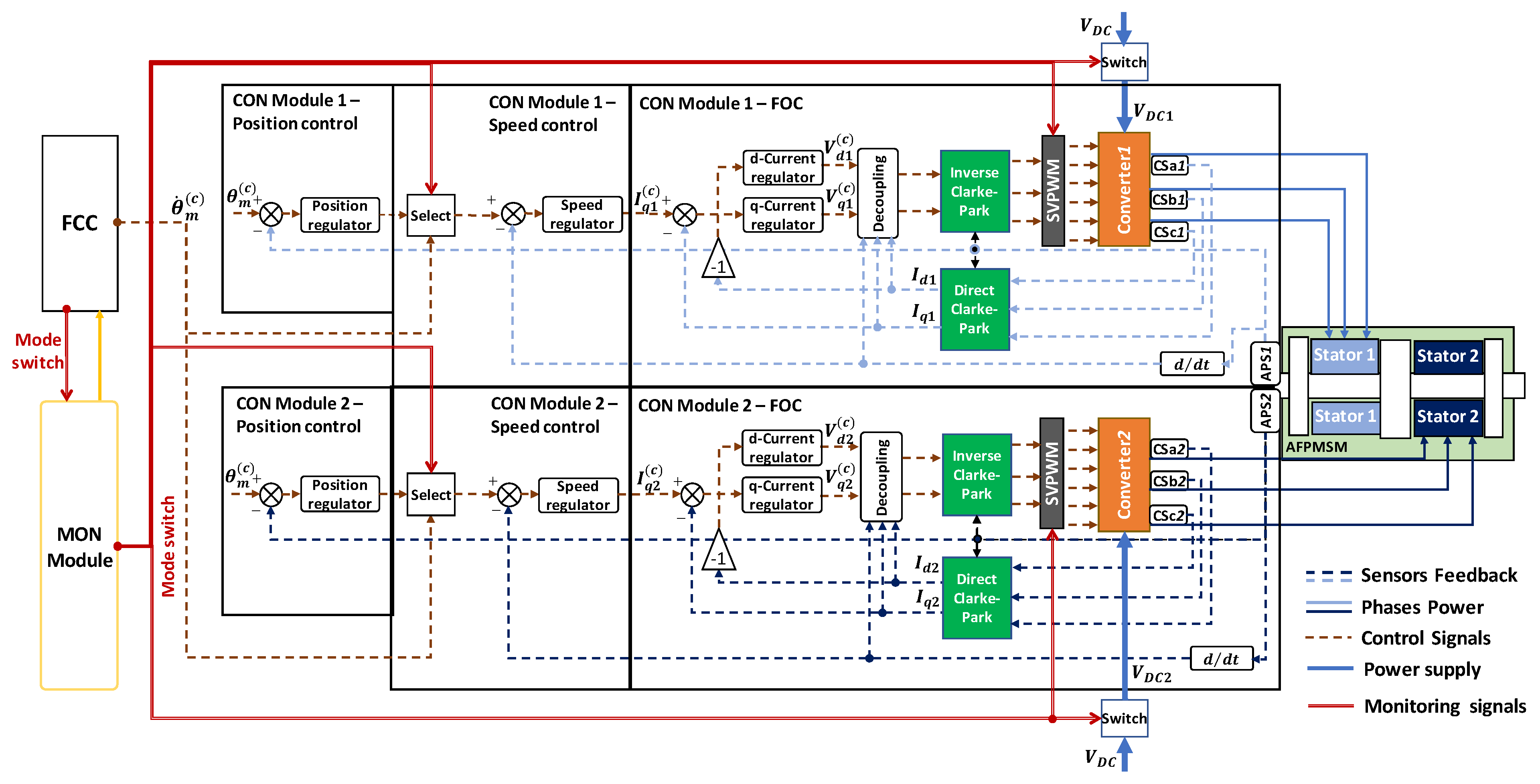
2.1. System Description

The reference FEPS is essentially composed of (Figure 2) a surface-mounted magnet AFPMSM with a double-stator having phases in star connection. The AFPMSM rotor is connected mechanically via a coupling joint to a twin-blade fixed-pitch propeller (APC22 × 10E [34]) generating the UAV thrust. Electrically, the AFPMSM is connected to two Electronic Control Units (ECUs), including a Control/Monitoring (CON/MON) module, a three-leg converter, a Power Supply Unit (PSU), and an I/O interface. The I/O connectors exchange data with the Flight Control Computer (FCC) and receive the electrical power input and the control feedbacks from the three Current Sensors (CSa, CSb, CSc) and the Angular Position Sensors (APS).

The closed-loop control of the system is implemented by the CON module, via two cascade loops, on propeller speed and motor currents (via Field-Oriented Control, FOC). The regulators are proportional/integral, including back-calculation anti-windup actions.

2.2. Modelling with Demagnetization and Angular Misalignment

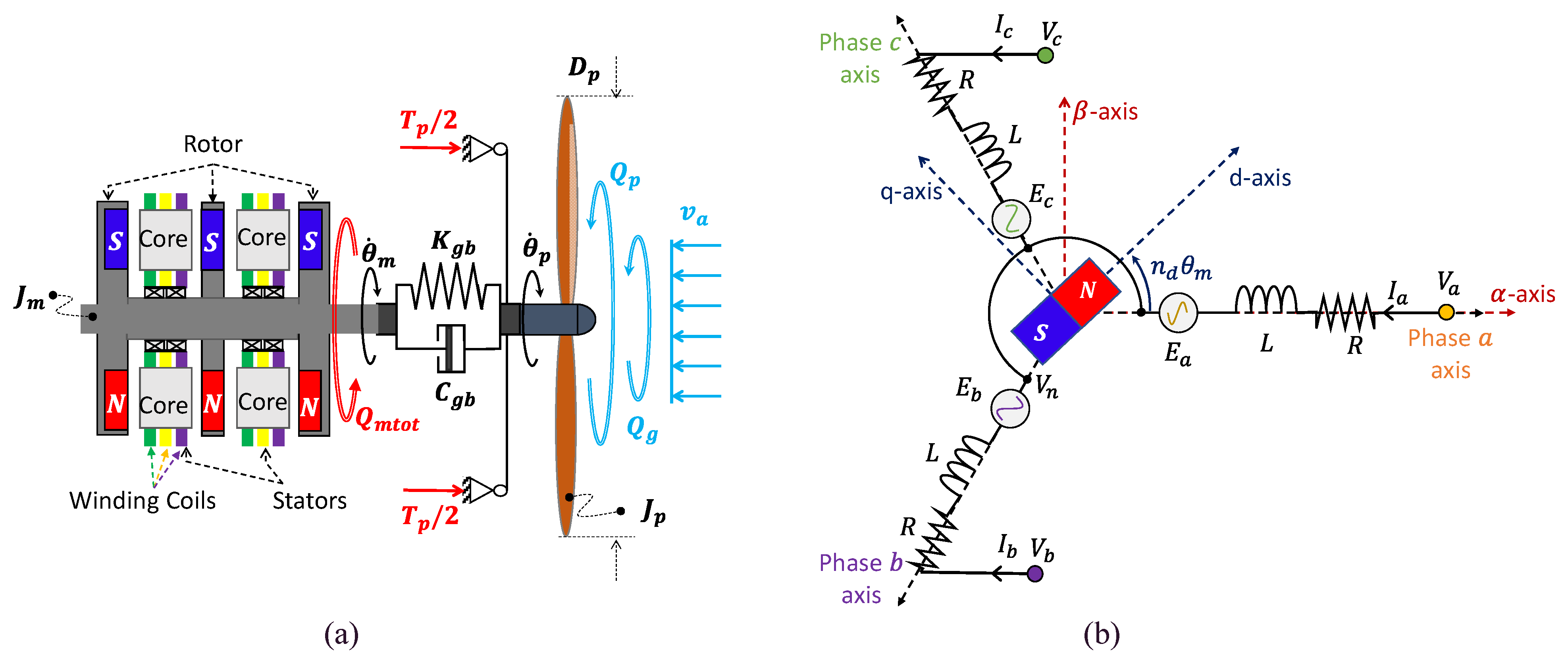
2.2.1. Aero-Mechanical Modelling

The aero-mechanical section of the FEPS model aims to calculate the UAV thrust force ($T_p$) once the altitude (i.e., the air density $\rho$), the vehicle forward speed ($v_a$), the gust-induced torque ($Q_g$), and the electrical motor torque generated by the two stator modules ($Q_{m\mathrm{tot}}$) are known, Equation (1) [10,14], Figure 3a:

$$\{\begin{array}{c}{J}_p{\ddot{\theta }}_p=-Q_p-C_{gb}\left({\dot{\theta }}_p-{\dot{\theta }}_m\right)-K_{gb}\left({\theta }_p-{\theta }_m\right)+Q_g\\ J_m{\ddot{\theta }}_m=Q_{m\mathrm{tot}}+C_{gb}\left({\dot{\theta }}_p-{\dot{\theta }}_m\right)+K_{gb}\left({\theta }_p-{\theta }_m\right)\\ Q_p=C_Q\left({\dot{\theta }}_p,AR\right)\rho D_p^5{\dot{\theta }}_p^2\\ T_p=C_T\left({\dot{\theta }}_p,AR\right)\rho D_p^4{\dot{\theta }}_p^2 \\ AR=2\pi v_a/D_p{\dot{\theta }}_p\end{array},$$

(1)

where $J_p$ and $J_m$ are the propeller and motor inertias, ${\theta }_p$ and ${\theta }_m$ are the propeller and motor rotations, $D_p$ is the propeller diameter, $AR$ is the propeller advance ratio, $Q_p$ is the propeller resistant torque, $C_Q$ and $C_T$ are the torque and thrust propeller coefficients (Figure 4), and $K_{gb}$ and $C_{gb}$ are the torsional stiffness and damping of the coupling joint.

2.2.2. Electrical Modelling of the Single Stator

The current dynamics in the single stator module can be described in vectorized form by [5,15], Figure 3b:

$$V_{abc}=R{I}_{abc}+L{\dot{I}}_{abc}+E_{abc},$$

(2)

$$E_{abc}=\left(1-{\alpha }_m\right)k_m{\dot{\theta }}_m{\mathit{e}}_{abc},$$

(3)

in which $V_{abc}={\left[V_a-V_n,V_b-V_n,V_c-V_n\right]}^T$ is the applied voltages vector, $I_{abc}={\left[I_a, I_b, I_c\right]}^T$ is the stator currents vector, $E_{abc}$ is the Back Electromotive Force (BEMF) vector, $R$ and $L$ are the resistance and inductance of the phases, $k_m$ is the motor speed constant, ${\mathit{e}}_{abc}={\left[e_a, e_b, e_c\right]}^T$ is the BEMF waveforms vector, and ${\alpha }_m$ is the uniform demagnetization factor ($0\le {\alpha }_m\le 1$, where ${\alpha }_m$ = 0 applies to the nominal design, while ${\alpha }_m$ = 1 means no magnetic coupling). The parameters and data related to the propulsion system model are reported in Appendix A.

In case of sinusoidal magnetic coupling and uniform demagnetization, we have:

$$e_a=\sin \left(n_d{\theta }_m\right), e_b= \sin \left(n_d{\theta }_m-\frac{2}{3}\pi \right), e_c= \sin \left(n_d{\theta }_m+\frac{2}{3}\pi \right)$$

(4)

where $n_d$ is the number of pole pairs.

The analysis of three-phase PMSMs is conventionally carried out by calculating magnetic and electrical quantities in the rotating reference frame (($d,q,z$) in Figure 3b) and by applying the Clarke–Park transformations [15] so that, once we have defined the stator-referenced vector $x_{abc}$ and the electrical angle ${\theta }_e$ between rotor and stator, we have

$$x_{\alpha \beta \gamma }={\mathbb{T}}_C{x}_{abc}=\sqrt{\frac{2}{3}}\left[\begin{array}{ccc}1& -1/2& -1/2\\ 0& \sqrt{3}/2& -\sqrt{3}/2\\ \sqrt{2}/2& \sqrt{2}/2& \sqrt{2}/2\end{array}\right]x_{abc},$$

(5)

$$x_{dqz}={\mathbb{T}}_P{x}_{\alpha \beta \gamma }=\left[\begin{array}{ccc}\cos {\theta }_e& \sin {\theta }_e& 0\\ -\sin {\theta }_e& \cos {\theta }_e& 0\\ 0& 0& 1\end{array}\right]x_{\alpha \beta \gamma }={\mathbb{T}}_P{\mathbb{T}}_C{x}_{abc}={\mathbb{T}}_{PC}{x}_{abc}.$$

(6)

Taking into account an electrical angle delay $\phi$, so that ${\theta }_e=n_d{\theta }_m-\phi$, ${\mathbb{T}}_{PC}$ becomes

$${\mathbb{T}}_{PC}=\sqrt{\frac{2}{3}}\left[\begin{array}{ccc}\cos \left(n_d{\theta }_m-\phi \right)& \cos \left(n_d{\theta }_m-\frac{2\pi }{3}-\phi \right)& \cos \left(n_d{\theta }_m+\frac{2\pi }{3}-\phi \right)\\ -\sin \left(n_d{\theta }_m-\phi \right)& -\sin \left(n_d{\theta }_m-\frac{2\pi }{3}-\phi \right)& -\sin \left(n_d{\theta }_m+\frac{2\pi }{3}-\phi \right)\\ \sqrt{2}/2& \sqrt{2}/2& \sqrt{2}/2\end{array}\right],$$

(7)

which can be conveniently formulated as:

$${\mathbb{T}}_{PC}=\cos \phi {{\mathbb{T}}_{PC}^{ }|}_{\phi =0}+\sin \phi {\mathbb{M}}_a,$$

(8)

where:

$${\mathbb{M}}_a=\sqrt{\frac{2}{3}}\left[\begin{array}{ccc}\sin \left(n_d{\theta }_m\right)& \sin \left(n_d{\theta }_m-\frac{2\pi }{3}\right)& \sin \left(n_d{\theta }_m+\frac{2\pi }{3}\right)\\ \cos \left(n_d{\theta }_m\right)& \cos \left(n_d{\theta }_m-\frac{2\pi }{3}\right)& \cos \left(n_d{\theta }_m+\frac{2\pi }{3}\right)\\ \frac{\sqrt{2}\left(1-\cos \phi \right)}{2\sin \phi }& \frac{\sqrt{2}\left(1-\cos \phi \right)}{2\sin \phi }& \frac{\sqrt{2}\left(1-\cos \phi \right)}{2\sin \phi }\end{array}\right].$$

(9)

For any stator-referenced vector $x_{abc}$ we actually have:

$$\begin{array}{c}{x}_{dqz}={\mathbb{T}}_{PC}{x}_{abc}=\left(\cos \phi {{\mathbb{T}}_{PC}^{ }|}_{\phi =0}+\sin \phi {\mathbb{M}}_a\right){\left({{\mathbb{T}}_{PC}^{ }|}_{\phi =0}\right)}^T{x_{dqz}|}_{\phi =0}=\dots \\ =\left\{\cos \phi +\sin \phi \left[\begin{array}{ccc}0& -1& 0\\ 1& 0& 0\\ 0& 0& \frac{\sqrt{3}\left(1-\cos \phi \right)}{\sqrt{2}\sin \phi }\end{array}\right]\right\}{x_{dqz}|}_{\phi =0},\end{array}$$

(10)

in which ${x_{dqz}|}_{\phi =0}$ represents the Clark–Park transformation of the vector $x_{abc}$ without angle delay. The electrical equation in the rotating–delayed frame is structurally identical to the ideal case,

$$V_{dqz}=R{I}_{dqz}+L{\dot{I}}_{dqz}+L{n}_d{\dot{\theta }}_m\left[\begin{array}{ccc}0& -1& 0\\ 1& 0& 0\\ 0& 0& 0\end{array}\right]I_{dqz}+E_{dqz},$$

(11)

except that:

$$\begin{array}{c}{E}_{dqz}={\mathbb{T}}_{PC}{E}_{abc}={\mathbb{T}}_{PC}{\left({{\mathbb{T}}_{PC}^{ }|}_{\phi =0}\right)}^{-1}{E_{dqz}|}_{\phi =0}=\dots \\ =\left(1-{\alpha }_m\right)k_m{\dot{\theta }}_m{\mathbb{T}}_{PC}{\left({{\mathbb{T}}_{PC}^{ }|}_{\phi =0}\right)}^T\left[\begin{array}{c}0\\ 1\\ 0\end{array}\right]=\left(1-{\alpha }_m\right)k_m{\dot{\theta }}_m\left[\begin{array}{c}-\sin \phi \\ \cos \phi \\ 0\end{array}\right]\end{array}.$$

(12)

It is worth noting that the electrical angle delay $\phi$ is composed of two main contributions: one (${\delta }_a$) related to the angular sensor misalignment and the other ($\gamma$), which can be important when high-speed applications are concerned, due to the computational delay of the control electronics operating at sample time $T_s$ (“zero-order hold” effect [35]):

$$\phi ={\delta }_a+\gamma ={\delta }_a+n_d{\dot{\theta }}_m{T}_s/2,$$

(13)

If the computational delay is predictable and can be eliminated by applying a compensating lead (${\gamma }^{\prime }=n_d{\dot{\theta }}_m{T}_s/2$), the angular sensor misalignment is non-deterministic, as it can be caused by bias or degradations, Equation (14)

$$\phi ={\delta }_a+\gamma -{\gamma }^{\prime }\approx {\delta }_a.$$

(14)

The equation describing the current dynamics in both modules can be generally expressed by Equation (15), provided that the respective values of ${\alpha }_m$ and ${\delta }_a$ are used:

$$\{\begin{array}{c}{V}_d=R{I}_d+L{\dot{I}}_d-L{n}_d{\dot{\theta }}_m{I}_q-\left(1-{\alpha }_m\right)k_m{\dot{\theta }}_m\sin {\delta }_a\\ V_q=R{I}_q+L{\dot{I}}_q+L{n}_d{\dot{\theta }}_m{I}_d+\left(1-{\alpha }_m\right)k_m{\dot{\theta }}_m\cos {\delta }_a\end{array}.$$

(15)

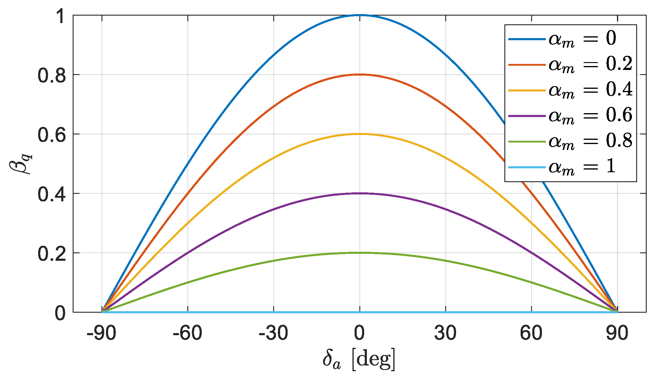
2.2.3. Torque Imbalance between Modules with Angular Misalignment and Demagnetization

In the reference application, the FEPS control system (Figure 5) applies a current-motion decoupling technique, which, once given the current regulator outputs $V_d^{\left(c\right)}$ and $V_q^{\left(c\right)}$, defines the direct and quadrature voltages as

$$\{\begin{array}{c}{V}_d=V_d^{\left(c\right)}-L{n}_d{\dot{\theta }}_m{I}_q\\ V_q=V_q^{\left(c\right)}+L{n}_d{\dot{\theta }}_m{I}_d\end{array},$$

(16)

so that the electrical equations become:

$$\{\begin{array}{c}{V}_d^{\left(c\right)}=R{I}_d+L{\dot{I}}_d-\left(1-{\alpha }_m\right)k_m{\dot{\theta }}_m\sin {\delta }_a\\ V_q^{\left(c\right)}=R{I}_q+L{\dot{I}}_q+\left(1-{\alpha }_m\right)k_m{\dot{\theta }}_m\cos {\delta }_a\end{array}.$$

(17)

Following a typical design solution, the current regulators are proportional–integral, so, once defined $k_p$ and $k_p{z}_I$ the proportional and integral gains, in the Laplace domain we have ($s$ is the complex pulsation):

$$\{\begin{array}{c}{V}_d^{\left(c\right)}=-k_p\frac{\left(s+z_I\right)}{s}{I}_d\\ V_q^{\left(c\right)}=k_p\frac{\left(s+z_I\right)}{s}\left(I_q^{\left(c\right)}-I_q\right)\end{array}.$$

(18)

The direct and quadrature currents responses for both modules can be obtained as:

$$\{\begin{array}{c}{I}_d\left(s\right)=\frac{{\beta }_d{k}_{m}s}{\left(Ls+R\right)s+k_p\left(s+z_I\right)}{\dot{\theta }}_m\left(s\right)\\ I_q\left(s\right)=\frac{k_p\left(s+z_I\right)}{\left(Ls+R\right)s+k_p\left(s+z_I\right)}{I}_q^{\left(c\right)}\left(s\right)-\frac{{\beta }_q{k}_{m}s}{\left(Ls+R\right)s+k_p\left(s+z_I\right)}{\dot{\theta }}_m\left(s\right)\end{array},$$

(19)

where

$$\{\begin{array}{c}{\beta }_d=\left(1-{\alpha }_m\right)sin{\delta }_a\\ {\beta }_q=\left(1-{\alpha }_m\right)cos{\delta }_a\end{array}$$

(20)

By neglecting cogging torque disturbances, the electrical torque generated by the single stator module ($Q_m$), is given by:

$$Q_m=\sqrt{3/2}{k}_m\left(1-{\alpha }_m\right)\left(I_{q}cos{\delta }_a-I_{d}sin{\delta }_a\right),$$

(21)

To simplify the discussion, let us assume that one of the two modules works with angular sensor misalignment and demagnetization, while the other is normally operating; the total motor torque ($Q_{m\mathrm{tot}}$) and the torque imbalance between modules ($Q_{mi}$) are expressed by

$$\{\begin{array}{c}{Q}_{m\mathrm{tot}}=\sqrt{3/2}{k}_m\left({\beta }_q{I}_q-{\beta }_d{I}_d+{I_q|}_{{\delta }_a=0;{\alpha }_m=0}\right)\\ Q_{mi}=\sqrt{3/2}{k}_m\left({\beta }_q{I}_q-{\beta }_d{I}_d-{I_q|}_{{\delta }_a=0;{\alpha }_m=0}\right)\end{array}.$$

(22)

By substituting Equation (19) into Equation (22), we obtain in the Laplace domain,

$$Q_{m\mathrm{tot}}\left(s\right)=\sqrt{\frac{3}{2}}{k}_m\left\{\frac{\left({\beta }_q+1\right)k_p\left(s+z_I\right)}{\left(Ls+R\right)s+k_p\left(s+z_I\right)}{I}_q^{\left(c\right)}\left(s\right)-\frac{\left[{\left(1-{\alpha }_m\right)}^2+1\right]k_{m}s}{\left(Ls+R\right)s+k_p\left(s+z_I\right)}{\dot{\theta }}_m\left(s\right)\right\}$$

(23)

$$Q_{mi}\left(s\right)=\sqrt{\frac{3}{2}}{k}_m\left\{\frac{\left({\beta }_q-1\right)k_p\left(s+z_I\right)}{\left(Ls+R\right)s+k_p\left(s+z_I\right)}{I}_q^{\left(c\right)}\left(s\right)-\frac{\left[{\left(1-{\alpha }_m\right)}^2-1\right]k_{m}s}{\left(Ls+R\right)s+k_p\left(s+z_I\right)}{\dot{\theta }}_m\left(s\right)\right\}$$

(24)

To generalize the concept wrt to the specific motor design, it is worth noting that Equations (23) and (24) can be reformulated as follows

$$Q_{m\mathrm{tot}}\left(s\right)=\sqrt{\frac{3}{2}}{k}_m{H}_{II}\left(s\right)\left\{\left({\beta }_q+1\right)I_q^{\left(c\right)}\left(s\right)-\frac{k_m\left[{\left(1-{\alpha }_m\right)}^2+1\right]}{k_p\left(s+z_I\right)}{\ddot{\theta }}_m\left(s\right)\right\}$$

(25)

$$Q_{mi}\left(s\right)=\sqrt{\frac{3}{2}}{k}_m{H}_{II}\left(s\right)\left\{\left({\beta }_q-1\right)I_q^{\left(c\right)}\left(s\right)-\frac{k_m\left[{\left(1-{\alpha }_m\right)}^2-1\right]}{k_p\left(s+z_I\right)}{\ddot{\theta }}_m\left(s\right)\right\}$$

(26)

where $H_{II}\left(s\right)$ is the current-tracking transfer function (always assuming a unity value for $s\to 0$), depending on the specific motor design and related control loop.

Equations (25) and (26) point out the detrimental effects of ${\alpha }_m$ and ${\delta }_a$ on propulsion-system efficiency. The demagnetization and the erroneous application of an FOC technique actually induce a torque imbalance between the modules and a reduction in the total torque capability. In particular, at constant motor speed (${\ddot{\theta }}_m=0$, an operative condition covering most of flight mission time), the torque responses depend on the term ${\beta }_q$ (Figure 6), which can be viewed as the torque capability index of the demagnetized and misaligned stator. When the torque capability reduces, the outer control loop, in pursuing the propeller speed tracking, increases the demand current $I_q^{\left(c\right)}$ to recover torque, but it also surges the torque imbalance. As a final result, the system works at higher currents, higher temperatures, and lower efficiency, and the speed tracking bandwidth diminishes.

The above discussion permits us to outline the importance of obtaining online estimates of the ${\delta }_a$ and ${\alpha }_m$, which can be used for both diagnostic and prognostic purposes.

A generalized formulation of Equations (25) and (26) can be finally obtained by considering both modules affected by degradations, leading to

$$Q_{m\mathrm{tot}}\left(s\right)=\sqrt{\frac{3}{2}}{k}_m{H}_{II}\left(s\right)\left\{\left({\beta }_{q1}+{\beta }_{q2}\right)I_q^{\left(c\right)}\left(s\right)-\frac{k_m\left[{\left(1-{\alpha }_{m1}\right)}^2+{\left(1-{\alpha }_{m2}\right)}^2\right]s}{k_p\left(s+z_I\right)}{\dot{\theta }}_m\left(s\right)\right\}$$

(27)

$$Q_{mi}\left(s\right)=\sqrt{\frac{3}{2}}{k}_m{H}_{II}\left(s\right)\left\{\left({\beta }_{q1}-{\beta }_{q2}\right)I_q^{\left(c\right)}\left(s\right)-\frac{k_m\left[{\left(1-{\alpha }_{m1}\right)}^2+{\left(1-{\alpha }_{m2}\right)}^2\right]s}{k_p\left(s+z_I\right)}{\dot{\theta }}_m\left(s\right)\right\}$$

(28)

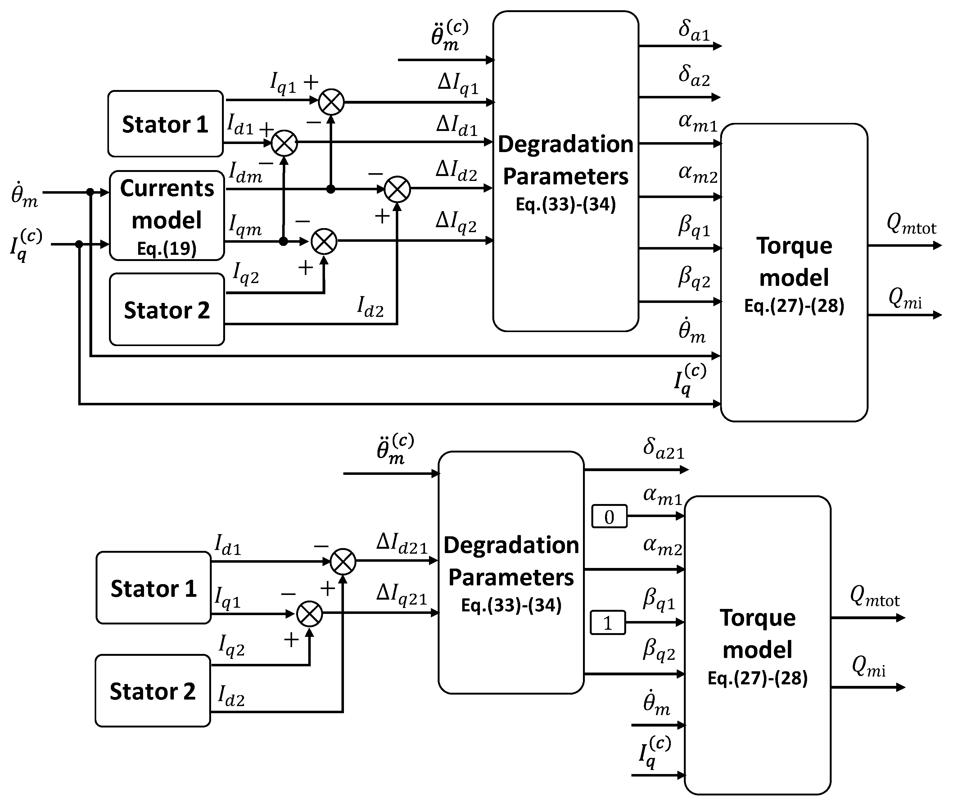
2.3. Monitoring of Demagnetization and Angular Misalignment

Equation (19) applied for ${\delta }_a=0;{\alpha }_m=0$ predict direct and quadrature currents for the nominal operation of a stator, so that the direct and quadrature current deviations from the nominal behaviour ($\mathsf{\Delta }{I}_d$ and $\mathsf{\Delta }{I}_q$) are

$$\{\begin{array}{c}\mathsf{\Delta }{I}_d\left(s\right)=I_d-{I_d|}_{{\delta }_a=0;{\alpha }_m=0}=\frac{{\beta }_d{k}_{m}s}{\left(Ls+R\right)s+k_p\left(s+z_I\right)}{\dot{\theta }}_m\left(s\right)\\ \mathsf{\Delta }{I}_q\left(s\right)=I_q-{I_q|}_{{\delta }_a=0;{\alpha }_m=0}=\frac{\left(1-{\beta }_q\right)k_{m}s}{\left(Ls+R\right)s+k_p\left(s+z_I\right)}{\dot{\theta }}_m\left(s\right)\end{array}$$

(29)

When the motor works at constant acceleration $A_m$, i.e.,

$${\dot{\theta }}_m\left(t\right)=A_{m}t \stackrel{ℒ}{\to } {\dot{\theta }}_m\left(s\right)=\frac{A_m}{s^2},$$

(30)

the two signals $\mathsf{\Delta }{I}_d$ and $\mathsf{\Delta }{I}_q$ reach finite steady-state values given by

$$\{\begin{array}{c}\mathsf{\Delta }{I}_{d\infty }=\underset{t\to \infty }{\lim }\mathsf{\Delta }{I}_d\left(t\right)=\underset{s\to 0}{\lim }s\mathsf{\Delta }{I}_d\left(s\right)=\underset{s\to 0}{\lim }\frac{{\beta }_d{k}_m{A}_m}{\left(Ls+R\right)s+k_p\left(s+z_I\right)}=\frac{{\beta }_d{k}_m{A}_m}{k_p{z}_I}\\ \mathsf{\Delta }{I}_{q\infty }=\underset{t\to \infty }{\lim }\mathsf{\Delta }{I}_q\left(t\right)=\underset{s\to 0}{\lim }s\mathsf{\Delta }{I}_q\left(s\right)=\underset{s\to 0}{\lim }\frac{\left(1-{\beta }_q\right)k_m{A}_m}{\left(Ls+R\right)s+k_p\left(s+z_I\right)}=\frac{\left(1-{\beta }_q\right)k_m{A}_m}{k_p{z}_I}\end{array}$$

(31)

The measurements of direct and quadrature current deviations from the nominal behaviour ($\mathsf{\Delta }{I}_d$ and $\mathsf{\Delta }{I}_q$) can be thus used to calculate approximating values of ${\beta }_d$ and ${\beta }_q$

$$\{\begin{array}{c}{\beta }_d\approx \frac{k_p{z}_I}{\begin{array}{c}{k}_m\end{array}}·\frac{\mathsf{\Delta }{I}_d}{{\ddot{\theta }}_m^{\left(c\right)}}\\ {\beta }_q\approx 1-\frac{k_p{z}_I}{\begin{array}{c}{k}_m\end{array}}·\frac{\mathsf{\Delta }{I}_q}{{\ddot{\theta }}_m^{\left(c\right)}}\end{array}$$

(32)

where ${\ddot{\theta }}_m^{\left(c\right)}$ is the time derivative of the speed demand (${\dot{\theta }}_m^{\left(c\right)}$, Figure 5). Since Equation (32) cannot be solved during constant speed operation since ${\ddot{\theta }}_m^{\left(c\right)}$ = 0, estimates of ${\beta }_d$ and ${\beta }_q$ can be obtained via

$$\begin{array}{c}\left|{\ddot{\theta }}_m^{\left(c\right)}\right|\ge A_{mth} ⟹ \{\begin{array}{c}{\beta }_{de}=\frac{k_p{z}_I}{\begin{array}{c}{k}_m\end{array}}·\frac{\mathsf{\Delta }{I}_d}{{\ddot{\theta }}_m^{\left(c\right)}}\\ {\beta }_{qe}=1-\frac{k_p{z}_I}{\begin{array}{c}{k}_m\end{array}}·\frac{\mathsf{\Delta }{I}_q}{{\ddot{\theta }}_m^{\left(c\right)}}\end{array}\\ \left|{\ddot{\theta }}_m^{\left(c\right)}\right|<A_{mth} ⟹ \{\begin{array}{c}{\beta }_{de} \mathrm{not} \mathrm{defined}\\ {\beta }_{qe} \mathrm{not} \mathrm{defined}\end{array}\end{array}$$

(33)

in which $A_{mth}$ is an acceleration threshold.

The basic idea underlying the proposed monitoring technique is that the calculation of ${\beta }_{de}$ and ${\beta }_{qe}$ permits us to obtain online estimates of angle misalignment ${\delta }_{ae}$ and asymmetric demagnetization ${\alpha }_{me}$ of each stator via

$$\{\begin{array}{c}{\delta }_{ae}=\mathrm{atan}\left(\frac{{\beta }_{de}}{{\beta }_{qe}}\right)\\ {\alpha }_{me}=1-\sqrt{{\beta }_{de}^2+{\beta }_{qe}^2}\end{array}$$

(34)

so that total torque and torque imbalance of the motor can be evaluated, Equations (25) and (26).

Since the current tracking dynamics are characterized by high-frequency bandwidths, the applicability of this model-based technique [15] depends on the availability of adequate computational resources. Alternatively, the concept can be applied to develop a signal-based technique (Figure 7), provided that the terms ${I_d|}_{{\delta }_a=0;{\alpha }_m=0}$ and ${I_q|}_{{\delta }_a=0;{\alpha }_m=0}$ in Equation (26) are referring to measurements coming from one of the two. Clearly, the signal-based approach can only provide information about the asymmetries of demagnetization and electrical angle misalignment of the modules.

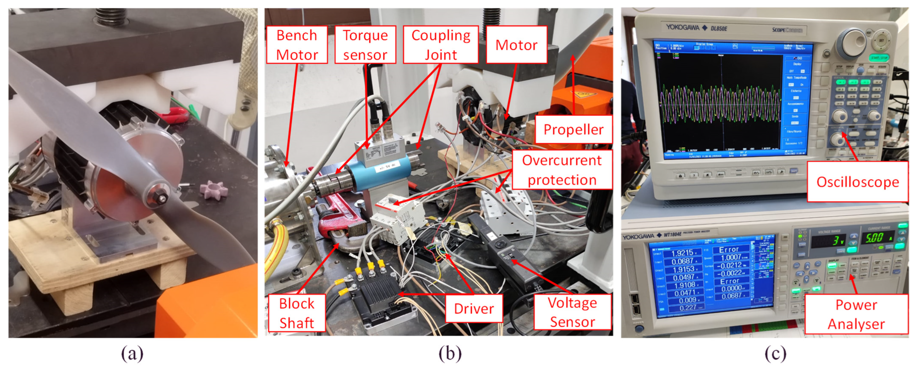
2.4. FEPS Prototype Test Plan

To characterize the FEPS basic performances, to identify/substantiate the main parameters of the FEPS model as well as to validate the closed-loop regulators, the following test campaigns have been carried out:

T1.

Single stator/dragged rotor/torque control: i.e., while the rotor is dragged at constant speed by an external motor, one of the two FEPS modules is controlled in torque, and the step inputs of the quadrature current are tracked. The test aimed to characterize the module efficiency as functions of speed and torque.

T2.

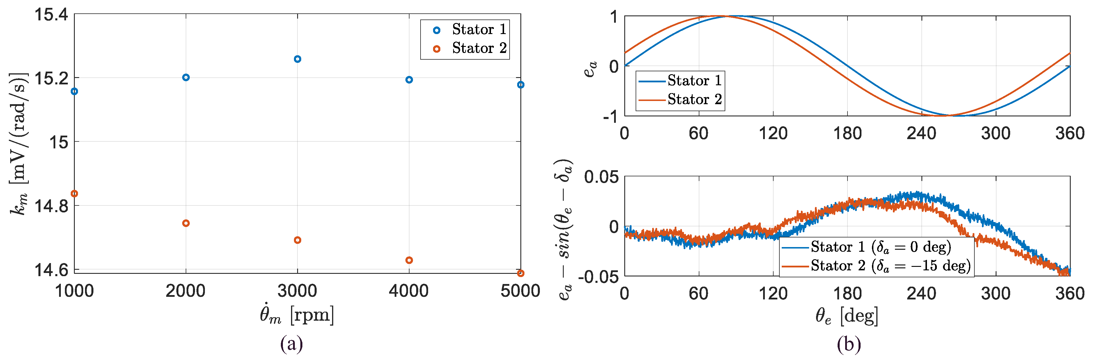
Dual stator/dragged rotor/open-phases: i.e., the rotor is dragged at a constant speed by an external motor with disconnected phases on both modules. The test aimed to identify the speed constant of the modules and the BEMF waveforms ($k_m$ and ${\mathit{e}}_{abc}$ in Equation (3)).

T3.

Single stator/blocked rotor/torque control: i.e., while the rotor is blocked, one of the two modules is controlled in torque, and step inputs of the quadrature current are tracked. The test aimed to identify the stator resistance and inductance ($R$ and $L$ in Equation (2)), as well as to validate the current regulators ($k_p$ and $z_I$ in Equation (18)).

T4.

Dual stator/coupled propeller/speed control: i.e., once the propeller is coupled to the rotor, one of the two modules is controlled in speed tracking and ramped-step inputs are given. The test aimed to identify the rotor inertia ($J_m$ in Equation (1)) and validate the speed regulators.

The main components of the experimental setup are (Figure 8):

• External motor: three-phase synchronous spindle motor SIEMENS 1FE1051-4HC30-1BA0 (nominal power 12.6 kW; nominal speed 24,000 rpm [36]);
• Torque sensor: Kistler 4503B (maximum torque 10 Nm [37]);
• Power analyser: Yokogawa WT 1804E [38];
• Oscilloscope: Yokogawa DL950 [39];
• Motor driver: BySTORM FTD50 [40].

3. Results

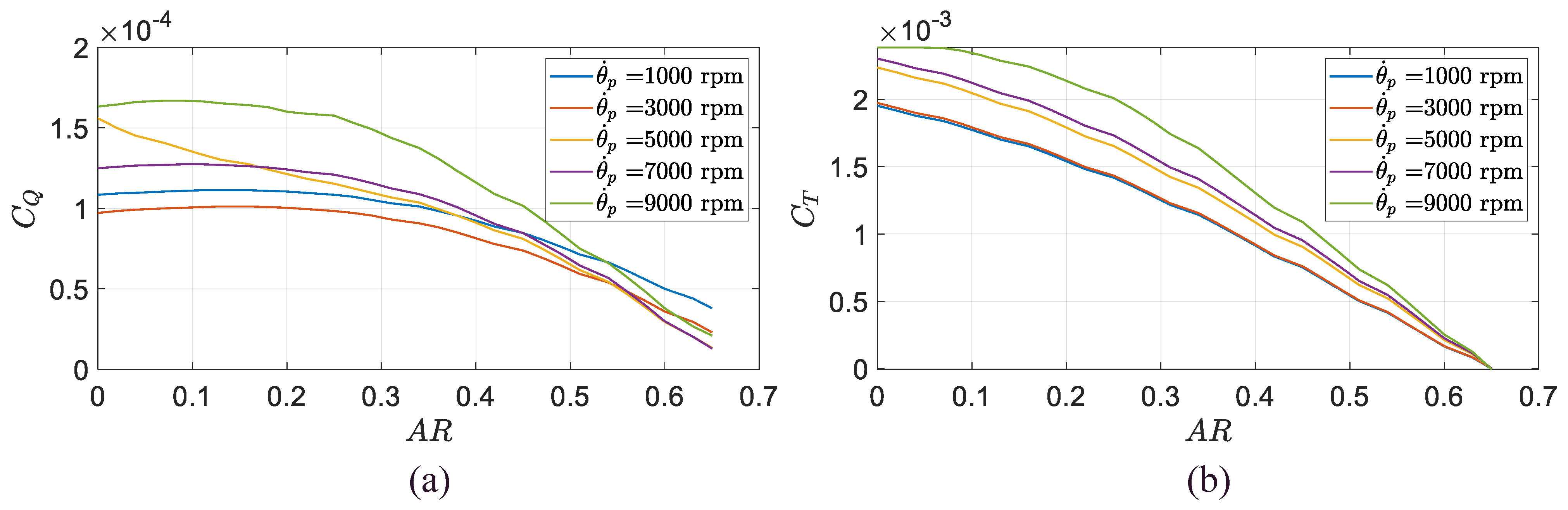
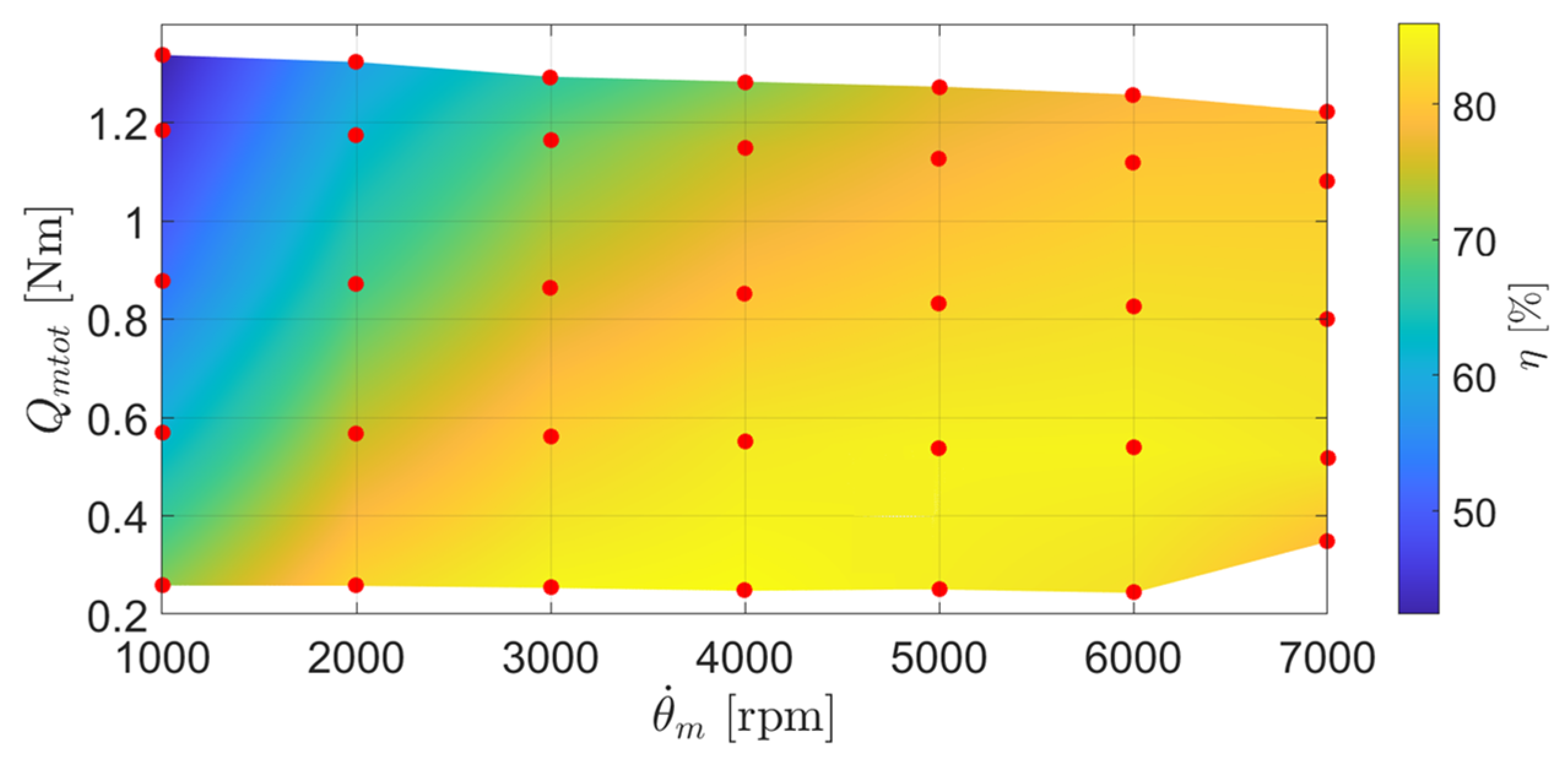
3.1. Open-Loop Performances

The motor efficiency ($\mathsf{\eta }$, Figure 9) is evaluated via T1 on a network of operating points defined in terms of speed and torque values. In particular, on each point, it is obtained by:

• imposing the rotor speed using the external speed-controlled motor;
• generating a resistant torque using the current-controlled FEPS module;
• measuring using the power signal analyser and the steady-state value of the ratio between the mechanical power output and electrical power input.

The tests have been executed from 1000 to 7000 rpm (with intervals of 1000 rpm) and from 10 to 45 A of quadrature current demands.

Figure 10 summarizes the results obtained via T2, in terms of speed constants, Figure 10a, and BEMF waveforms for both stator modules, Figure 10b. Experiments point out that the dependency of the speed constants on angular speed is negligible for both stator modules (verifying a model assumption), but the two stators have different speed constants: the mean value of $k_m$ for stator 1 is 0.0152 V s/rad, while it lowers to 0.0147 V s/rad for stator 2, Figure 10a. Assuming that the stator characterized by higher speed constant is the nominal one, this means that ${\alpha }_m$ = 0.03 for stator 2, Equation (2). The results obtained in terms of BEMF highlight that the waveforms are essentially sinusoidal (verifying a model assumption), but the two stators are characterized by relevant angular misalignment. Assuming stator 1 as the nominal one, this can be viewed as ${\delta }_a$ = −0.262 rad (about −15 deg) for stator 2, Equation (2), Figure 7b.

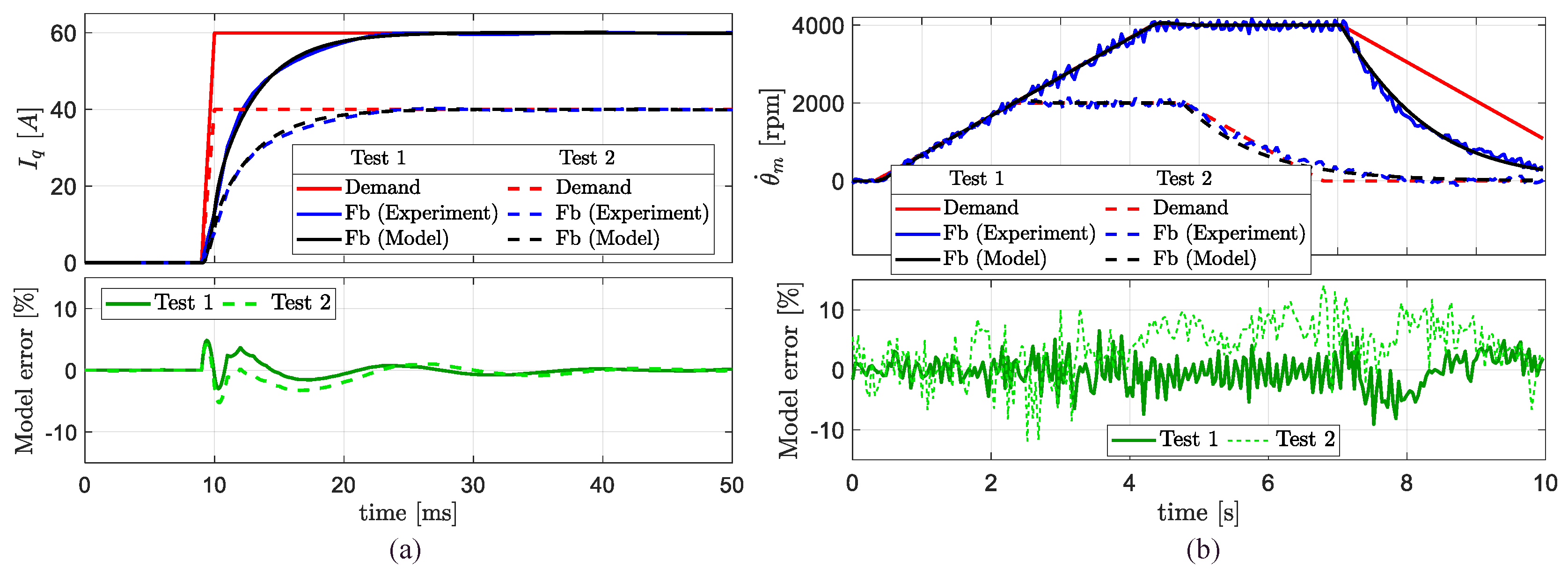
3.2. Closed-Loop Performances and Model Validation

An excerpt of the results coming from T3 and T4, related to the closed loop control validation, are reported in Figure 11. The validation is carried out by stimulating the hardware and the model with the same input requests, and by verifying that the deviations of their outputs are contained within pre-defined thresholds. Figure 11a documents the validation of the current tracking, obtained during T3, when requesting the step commands of the quadrature current (as an example: 40 A and 60 A in Figure 11a). The model provides very satisfactorily, with prediction errors lower than 5% wrt experiments. The speed-tracking validation is then reported in Figure 11b wrt T4, and it is accomplished by requesting ramped-step commands with 1000 rpm/s slopes (as an example, 2000 and 4000 rpm amplitude in Figure 11b). In these experiments, the test ends by removing the electrical power from the system in order to let the motor passively decelerate, thus permitting a more direct identification/substantiation of rotor inertia. Apart from a low-frequency harmonic disturbance at about 8 Hz, due to imperfect rig grounding, the model behaves very satisfactorily during both controlled and uncontrolled phases with a mean error of about 5%. It is worth noting that the model parameters are identified wrt the test at 4000 rpm (Test 1 in Figure 10), so that the errors tend to slightly increase at higher or lower commands.

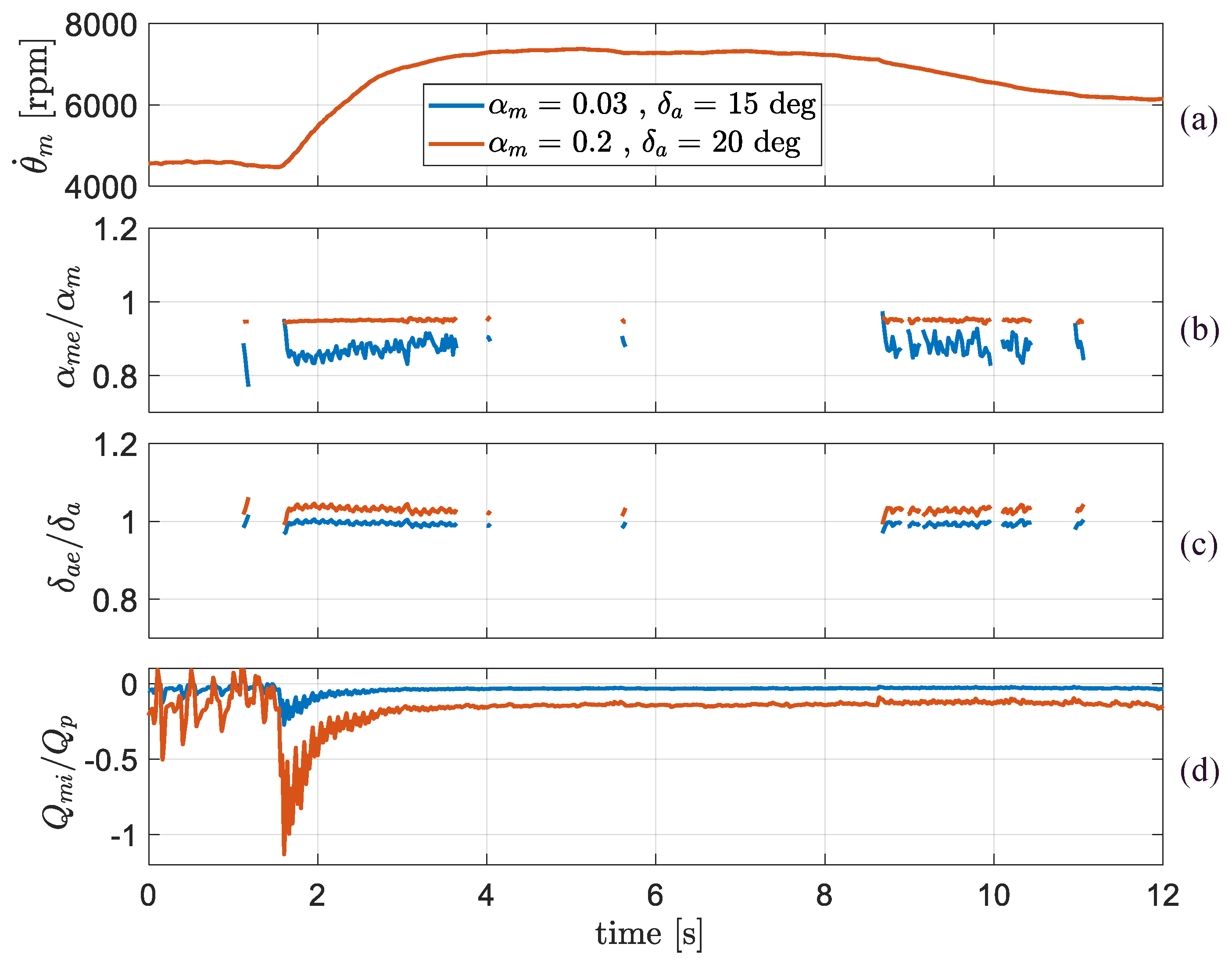
3.3. Characterization of Monitoring Performances via Nonlinear Simulation

To verify the effectiveness of the monitoring technique described in Section 2.4, two simulation test campaigns have been carried out with the experimentally validated model of the FEPS:

• firstly, by imposing speed requests characterized by constant acceleration;
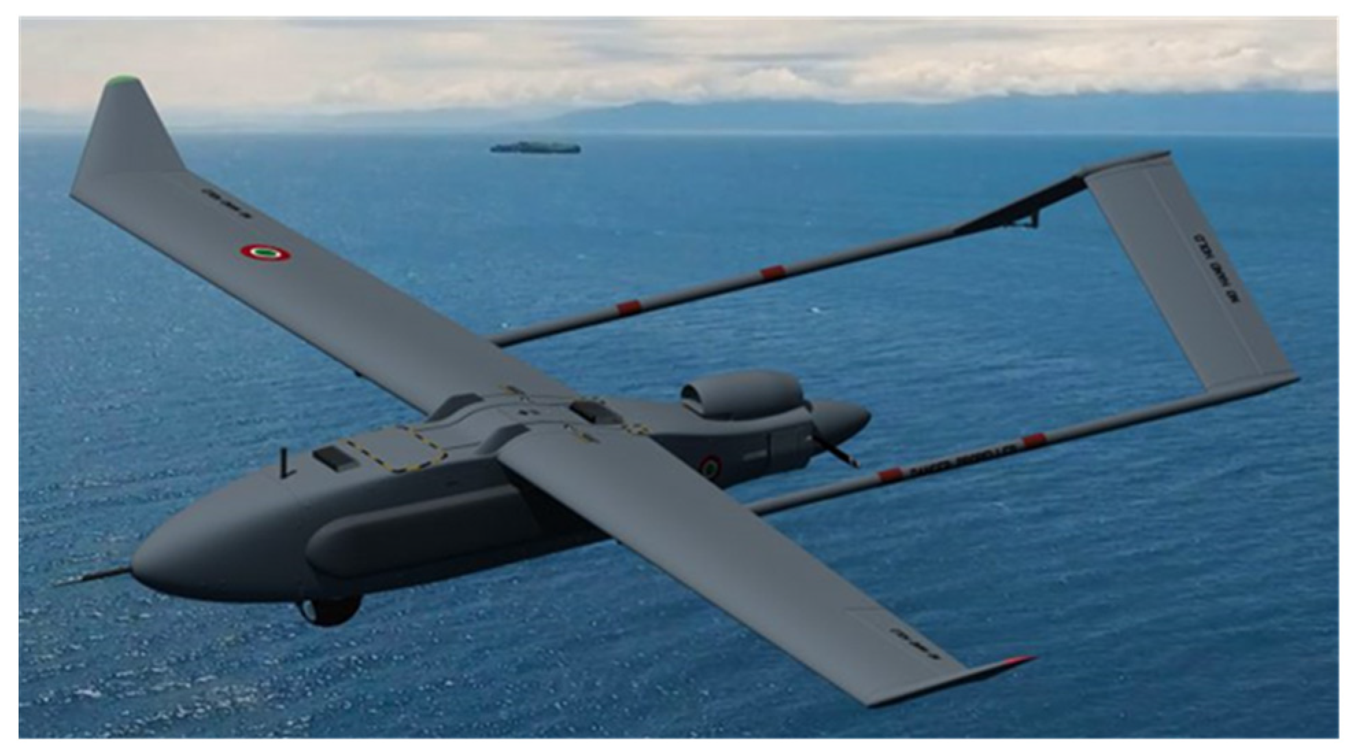
• secondly, by using the time history of the speed request recorded during a flight manoeuvre of the Rapier X-25 UAV by Sky Eye Systems (Italy), which (having similar architecture, weight, propeller, aerodynamics, and control systems) was the baseline solution for the development of the TERSA UAV.

The FEPS simulation is entirely developed in the MATLAB/Simulink environment, and its numerical solution is obtained via the fourth order Runge–Kutta method, using a 10⁻⁵ s integration step. The closed-loop control is executed at a 10 kHz sampling rate, while the monitoring function, being executed by the UAV flight control computer, provides outputs at 50 Hz sample rate.

3.3.1. Constant-Acceleration Testing

The results of the first session of tests for the monitoring technique verification is reported in Figure 12, in terms of speed command, monitoring outputs (estimations of demagnetization factor ${\alpha }_{me}$ and angle misalignment ${\delta }_{ae}$), and torque imbalance when different values of demagnetization factor ${\alpha }_m$ and angle misalignment ${\delta }_a$ are imposed on stator 2. For all test cases, the monitoring technique generates no outputs during constant speed operations, while during accelerations, it provides estimates of demagnetization and misalignment that rapidly converge (within about 500 ms) to the reference degradation. Concerning the torque imbalance ($Q_{mi}$), provided that its amplitude increases with the degradation level, it is essentially proportional to the aerodynamic torque ($Q_p$) when the motor speed is constant (t < 0.25 s and t > 2.25 s, Figure 12) and reaches a peak during the acceleration transient (t = 0.5 s, Figure 12). As outlined by the results, this parasitic loading can be relevant even at small degradation levels (at ${\alpha }_m$ = 0.05; ${\delta }_a$ = 5 deg, the imbalance amplitude ranges from 5% to 10% of the propeller torque).

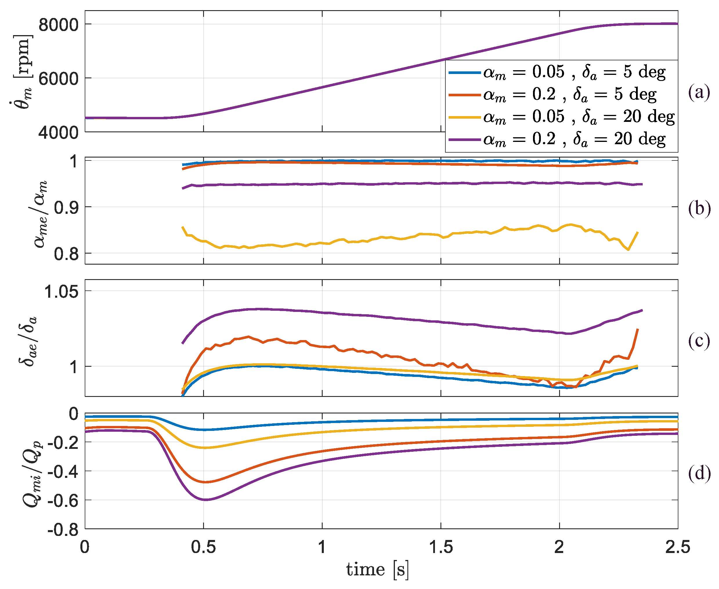
3.3.2. Flight Manoeuvre Testing

An excerpt of results obtained during the second session of tests is shown in Figure 13, where the estimations of the demagnetization factor and angle misalignment, as well as the torque imbalance, are reported in case the system is commanded by the time history of the speed request recorded during the climb flight manoeuvres of the Rapier X-25 UAV. The values of demagnetization factor ${\alpha }_m$ and angle misalignment ${\delta }_a$ of stator 2 are set to the measured ones (Section 3.1) and to the worst-case scenario analysed in Section 3.3.1. Based on Figure 13, we can see that even if the system exhibits torque unbalance the estimation of the parameters is realized only when the system accelerates over a certain threshold; in the other cases, the algorithm output is not defined.

4. Discussion

The results in Section 3 highlight the effectiveness and the potentialities of the proposed model-based monitoring for enhancing the reliability and performance of UAV FEPS with particular reference, but not limited, to architectures with redundant stators. Actually, provided that the computational resources of the onboard control electronics permit the simulation of the current tracking dynamics, the monitoring allows us to estimate the electrical angle misalignment and the demagnetization of the rotor magnet on each stator module. This information can then be used to evaluate the deviations in performances in terms of total torque capability (and torque imbalance, if redundant stators are concerned), with consequent capability to apply a control loop compensation. Conversely, if computational resources are limited, the concept can be applied to develop signal-based monitoring, even if, in this case, only the asymmetry of behaviour among modules could be evaluated. As far as the real-time execution capabilities are concerned, the computational burden of the algorithm has been evaluated in terms of the ratio between elapsed time of execution at 10 kHz rate and simulation time on a reference PC (DELL Inspiron 16 Plus 7620, 12th Gen Intel Core i7-12700H, 2.30 GHz, RAM 32 GB). If the model-based algorithm is executed, this ratio is 0.032 (i.e., the execution time is 3.2% of the real time), while if a signal-based algorithm is used, the ratio lowers to 0.028. These results point out that the computational resources required to run the algorithms are well-compatible with the real-time execution on UAV ECUs.

The basic limitations of the proposed monitoring technique are essentially related to the capability to only generate outputs during motor accelerations/decelerations; however, this feature is not critical, since the basic objective is not to diagnose a fault but to perform condition-monitoring of the system and be able to characterize degradations with long-term effects.

In terms of future development of the research, the estimation of demagnetization of a rotor-stator coupling throughout the FEPS lifecycle could be used for the design of prognostic algorithms that are able to anticipate detrimental effects on performance and to enhance reliability and maintainability. In addition, since the model-based monitoring has been designed and tested by neglecting cogging torque disturbances as well as local demagnetization, the sensitivity of these phenomena must be addressed.

5. Conclusions

A model-based technique for monitoring the torque imbalances of a redundant FEPS for UAVs is developed and verified through nonlinear simulations. The technique allows us to estimate the demagnetization and the electrical angle misalignment of each stator module using the measurements of direct and quadrature currents during motor accelerations. A propulsion system model, including degradations, is developed and validated with an FEPS prototype characterized by asymmetrical behaviour of the modules (errors are lower than about 5%). The basic limitation of the technique is that it operates during motor accelerations only; however, this does not impact the design objective, which is a condition-monitoring system for characterizing long-term degradations. The monitoring effectiveness is finally assessed by simulating UAV flight manoeuvres, injecting degradations, and evaluating the torque imbalance.

References

1. Chan, C.C. The State of the Art of Electric and Hybrid Vehicles. Proc. IEEE 2002, 90, 247–275. [Google Scholar] [CrossRef]
2. Zhang, B.; Song, Z.; Zhao, F.; Liu, C. Overview of Propulsion Systems for Unmanned Aerial Vehicles. Energies 2022, 15, 455. [Google Scholar] [CrossRef]
3. Suti, A.; Di Rito, G.; Galatolo, R. Climbing Performance Enhancement of Small Fixed-Wing UAVs via Hybrid Electric Propulsion. In Proceedings of the 2021 IEEE Workshop on Electrical Machines Design, Control and Diagnosis (WEMDCD), Modena, Italy, 8–9 April 2021; pp. 305–310. [Google Scholar]
4. Dici. Tersa. Available online: https://www.dici.unipi.it/progetti/tersa (accessed on 25 June 2023).
5. Suti, A.; Di Rito, G.; Galatolo, R. Fault-Tolerant Control of a Dual-Stator PMSM for the Full-Electric Propulsion of a Lightweight Fixed-Wing UAV. Aerospace 2022, 9, 337. [Google Scholar] [CrossRef]
6. Sky Eye Systems. Rapier X-Skysar. Available online: https://www.skyeyesystems.it/products/rapier-x-skysar/ (accessed on 15 July 2023).
7. Sudha, B.; Vadde, A.; Sachin, S. A Review: High Power Density Motors for Electric Vehicles. J. Phys. Conf. Ser. 2020, 1706, 012057. [Google Scholar] [CrossRef]
8. Bouaziz, O.; Jaafar, I.; Ammar, F.B. Performance Analysis of Radial and Axial Flux PMSM Based on 3D FEM Modeling. Turk. J. Electr. Eng. Comput. Sci. 2018, 26, 1587–1598. [Google Scholar] [CrossRef]
9. Cao, W.; Mecrow, B.C.; Atkinson, G.J.; Bennett, J.W.; Atkinson, D.J. Overview of Electric Motor Technologies Used for More Electric Aircraft (MEA). IEEE Trans. Ind. Electron. 2012, 59, 3523–3531. [Google Scholar] [CrossRef]
10. Suti, A.; Di Rito, G.; Galatolo, R. Fault-Tolerant Control of a Three-Phase Permanent Magnet Synchronous Motor for Lightweight UAV Propellers via Central Point Drive. Actuators 2021, 10, 253. [Google Scholar] [CrossRef]
11. STANAG 4671; Standardization Agreement—Unmanned Aerial Vehicles Systems Airworthiness Requirements (USAR). NATO: Brussels, Belgium, 2009.
12. Ryu, H.-M.; Kim, J.-W.; Sul, S.-K. Synchronous Frame Current Control of Multi-Phase Synchronous Motor Part II. Asymmetric Fault Condition Due to Open Phases. In Proceedings of the Conference Record of the 2004 IEEE Industry Applications Conference, 39th IAS Annual Meeting, Seattle, WA, USA, 3–7 October 2004; pp. 268–275. [Google Scholar]
13. Zhang, C.; Chen, F.; Li, L.; Xu, Z.; Liu, L.; Yang, G.; Lian, H.; Tian, Y. A Free-Piston Linear Generator Control Strategy for Improving Output Power. Energies 2018, 11, 135. [Google Scholar] [CrossRef]
14. Bennett, J.W.; Mecrow, B.C.; Atkinson, D.J.; Atkinson, G.J. Safety-Critical Design of Electromechanical Actuation Systems in Commercial Aircraft. IET Electr. Power Appl. 2011, 5, 37. [Google Scholar] [CrossRef]
15. Mazzoleni, M.; Di Rito, G.; Previdi, F. Electro-Mechanical Actuators for the More Electric Aircraft; Springer International Publishing: Cham, Switzerland, 2021; ISBN 978-3-030-61798-1. [Google Scholar]
16. Beltrao de Rossiter Correa, M.; Brandao Jacobina, C.; Cabral da Silva, E.R.; Nogueira Lima, A.M. An Induction Motor Drive System with Improved Fault Tolerance. IEEE Trans. Ind. Appl. 2001, 37, 873–879. [Google Scholar] [CrossRef]
17. Ribeiro, R.L.A.; Jacobina, C.B.; Lima, A.M.N.; da Silva, E.R.C. A Strategy for Improving Reliability of Motor Drive Systems Using a Four-Leg Three-Phase Converter. In Proceedings of the APEC 2001, Sixteenth Annual IEEE Applied Power Electronics Conference and Exposition, Anaheim, CA, USA, 4–8 March 2021; pp. 385–391. [Google Scholar]
18. Zhang, R.; Prasad, V.H.; Boroyevich, D.; Lee, F.C. Three-Dimensional Space Vector Modulation for Four-Leg Voltage-Source Converters. IEEE Trans. Power Electron. 2002, 17, 314–326. [Google Scholar] [CrossRef]
19. Mahmoudi, A.; Rahim, N.A.; Hew, W.P. Axial-Flux Permanent-Magnet Machine Modeling, Design, Simulation and Analysis. Sci. Res. Essays 2011, 6, 2525–2549. [Google Scholar]
20. Wang, Z.; Chen, J.; Cheng, M. Fault Tolerant Control of Double-Stator-Winding PMSM for Open Phase Operation Based on Asymmetric Current Injection. In Proceedings of the 2014 IEEE 17th International Conference on Electrical Machines and Systems (ICEMS), Hangzhou, China, 22–25 October 2014; pp. 3424–3430. [Google Scholar]
21. Baranski, M.; Szelag, W.; Jedryczka, C. Influence of Temperature on Partial Demagnetization of the Permanent Magnets during Starting Process of Line Start Permanent Magnet Synchronous Motor. In Proceedings of the 2017 IEEE International Symposium on Electrical Machines (SME), Naleczow, Poland, 18–21 June 2017; pp. 1–6. [Google Scholar]
22. McFarland, J.D.; Jahns, T.M. Influence of D- and q-Axis Currents on Demagnetization in PM Synchronous Machines. In Proceedings of the 2013 IEEE Energy Conversion Congress and Exposition, Denver, CO, USA, 15–19 September 2013; pp. 4380–4387. [Google Scholar]
23. Krichen, M.; Elbouchikhi, E.; Benhadj, N.; Chaieb, M.; Benbouzid, M.; Neji, R. Motor Current Signature Analysis-Based Permanent Magnet Synchronous Motor Demagnetization Characterization and Detection. Machines 2020, 8, 35. [Google Scholar] [CrossRef]
24. Ullah, Z.; Hur, J. A Comprehensive Review of Winding Short Circuit Fault and Irreversible Demagnetization Fault Detection in PM Type Machines. Energies 2018, 11, 3309. [Google Scholar] [CrossRef]
25. Sarikhani, A.; Mohammed, O. Demagnetization Control for Reliable Flux Weakening Control in PM Synchronous Machine. In Proceedings of the 2012 IEEE Industry Applications Society Annual Meeting, Las Vegas, NV, USA, 7–11 October 2012; pp. 1–8. [Google Scholar]
26. Galea, M.; Papini, L.; Zhang, H.; Gerada, C.; Hamiti, T. Demagnetization Analysis for Halbach Array Configurations in Electrical Machines. IEEE Trans. Magn. 2015, 51, 8107309. [Google Scholar] [CrossRef]
27. Cao, L.; Wu, Z. On-Line Detection of Demagnetization for Permanent Magnet Synchronous Motor via Flux Observer. Machines 2022, 10, 354. [Google Scholar] [CrossRef]
28. Moosavi, S.S.; Djerdir, A.; Amirat, Y.A.; Khaburi, D.A. Demagnetization Fault Diagnosis in Permanent Magnet Synchronous Motors: A Review of the State-of-the-Art. J. Magn. Magn. Mater. 2015, 391, 203–212. [Google Scholar] [CrossRef]
29. Xi, X.; Meng, Z.; Li, Y.; Li, M. On-Line Estimation of Permanent Magnet Flux Linkage Ripple for PMSM Based on a Kalman Filter. In Proceedings of the IECON 2006—32nd Annual Conference on IEEE Industrial Electronics, Paris, France, 7–10 November 2006; pp. 1171–1175. [Google Scholar]
30. Min, Y.; Huang, W.; Yang, J.; Zhao, Y. On-Line Estimation of Permanent-Magnet Flux and Temperature Rise in Stator Winding for PMSM. In Proceedings of the 2019 IEEE 22nd International Conference on Electrical Machines and Systems (ICEMS), Harbin, China, 11–14 August 2019; pp. 1–5. [Google Scholar]
31. Xu, W.; Jiang, Y.; Mu, C.; Blaabjerg, F. Improved Nonlinear Flux Observer-Based Second-Order SOIFO for PMSM Sensorless Control. IEEE Trans. Power Electron. 2019, 34, 565–579. [Google Scholar] [CrossRef]
32. Bobtsov, A.; Pyrkin, A.; Aranovskiy, S.; Nikolaev, N.; Slita, O.; Kozachek, O.; Quoc, D.V. Stator Flux and Load Torque Observers for PMSM. IFAC—Pap. OnLine 2020, 53, 5051–5056. [Google Scholar] [CrossRef]
33. Uddin, M.N.; Zou, H.; Azevedo, F. Online Loss-Minimization-Based Adaptive Flux Observer for Direct Torque and Flux Control of PMSM Drive. IEEE Trans. Ind. Appl. 2016, 52, 425–431. [Google Scholar] [CrossRef]
34. APC Propellers. Technical Info. Available online: https://www.apcprop.com/technical-information/performance-data/ (accessed on 20 May 2023).
35. Bae, B.-H.; Sul, S.-K. A Compensation Method for Time Delay of Full-Digital Synchronous Frame Current Regulator of PWM AC Drives. IEEE Trans. Ind. Appl. 2003, 39, 802–810. [Google Scholar] [CrossRef]
36. Siemens. Products & Services, Motors. Available online: https://www.siemens.com/global/en/products/drives/electric-motors/motion-control-motors/motor-spindles.html (accessed on 1 July 2023).
37. Kistler. Measure, Analyze, Innovate. Available online: https://www.kistler.com/it/it/cp/shaft-torque-sensors-4503b/p0000238 (accessed on 1 July 2023).
38. Yokogawa. Test & Measurement. Available online: https://tmi.yokogawa.com/solutions/products/power-analyzers/wt1800e-high-performance-power-analyzer/ (accessed on 1 July 2023).
39. Yokogawa. Test & Measurement. Available online: https://tmi.yokogawa.com/solutions/products/data-acquisition-equipment/high-speed-data-acquisition/dl950/ (accessed on 1 July 2023).
40. BySTORM & CO. Available online: https://bystorm.it/ftd50/ (accessed on 1 June 2023).
Figure 1. TERSA UAV.
Drones 07 00618 g001
Figure 2. Schematics of the FEPS control architecture.
Drones 07 00618 g002
Figure 3. FEPS modelling: (a) aero-mechanical reference scheme; (b) electrical reference scheme for the single three-phase stator module (one pole pair, n d = 1 ).
Drones 07 00618 g003
Figure 4. Torque coefficient (a) and thrust coefficient (b) as functions of propeller speed and advance ratio for the APC 18 × 22E propeller.
Drones 07 00618 g004
Figure 5. FEPS control system.
Drones 07 00618 g005
Figure 6. Torque capability index of a stator as a function of the demagnetization factor and misalignment angle.
Drones 07 00618 g006
Figure 7. Functional block diagrams for possible applications of the monitoring technique: model-based (top), signal-based (bottom).
Drones 07 00618 g007
Figure 8. Experimental setup: (a) coupled propeller; (b) rig layout; (c) equipment for signal analysis.
Drones 07 00618 g008
Figure 9. Experimental measurements of motor efficiency (single stator) as function of operating speed and torque.
Drones 07 00618 g009
Figure 10. Experimental measurements of BEMF parameters of stator 1 and stator 2: (a) speed constant as function of rotor speed; (b) BEMF waveforms as function of electrical angle.
Drones 07 00618 g010
Figure 11. Closed-loop control validation: (a) quadrature current tracking; (b) speed tracking.
Drones 07 00618 g011
Figure 12. Constant-acceleration test: motor speed (a), demagnetization factor estimate (b), angle misalignment estimate (c), and torque imbalance (d) at different values of demagnetization and misalignment of stator 2.
Drones 07 00618 g012
Figure 13. Flight manoeuvre test: motor speed (a), demagnetization factor estimate (b), angle misalignment estimate (c), and torque imbalance (d) at measured and worst-case values of demagnetization and misalignment of stator 2.
Drones 07 00618 g013
Disclaimer/Publisher’s Note: The statements, opinions and data contained in all publications are solely those of the individual author(s) and contributor(s) and not of MDPI and/or the editor(s). MDPI and/or the editor(s) disclaim responsibility for any injury to people or property resulting from any ideas, methods, instructions or products referred to in the content.