Abstract
When employing remote sensing images, it is challenging to classify vegetation species and ground objects due to the abundance of wetland vegetation species and the high fragmentation of ground objects. Remote sensing images are classified primarily according to their spatial resolution, which significantly impacts the classification accuracy of vegetation species and ground objects. However, there are still some areas for improvement in the study of the effects of spatial resolution and resampling on the classification results. The study area in this paper was the core zone of the Huixian Karst National Wetland Park in Guilin, Guangxi, China. The aerial images (Am) with different spatial resolutions were obtained by utilizing the UAV platform, and resampled images (An) with different spatial resolutions were obtained by utilizing the pixel aggregation method. In order to evaluate the impact of spatial resolutions and resampling on the classification accuracy, the Am and the An were utilized for the classification of vegetation species and ground objects based on the geographic object-based image analysis (GEOBIA) method in addition to various machine learning classifiers. The results showed that: (1) In multi-scale images, both the optimal scale parameter (SP) and the processing time decreased as the spatial resolution diminished in the multi-resolution segmentation process. At the same spatial resolution, the SP of the An was greater than that of the Am. (2) In the case of the Am and the An, the appropriate feature variables were different, and the spectral and texture features in the An were more significant than those in the Am. (3) The classification results of various classifiers in the case of the Am and the An exhibited similar trends for spatial resolutions ranging from 1.2 to 5.9 cm, where the overall classification accuracy increased and then decreased in accordance with the decrease in spatial resolution. Moreover, the classification accuracy of the Am was higher than that of the An. (4) When vegetation species and ground objects were classified at different spatial scales, the classification accuracy differed between the Am and the An.
1. Introduction
Wetlands are transition zones between terrestrial and aquatic ecosystems and are considered one of the three major ecological systems along with forests and oceans [1]. Moreover, they play a critical role in water conservation, water purification, flood storage, drought resistance, and the protection of biodiversity. Over the past half-century, excessive human activity has had a significant adverse impact on wetland ecosystems [2], with a large number of wetlands being converted into cropland, fishponds, and construction sites, resulting in a significant reduction in wetland areas [3,4]. In addition, the proliferation of croplands and fishponds contributes significantly to the pollution of wetland ecosystems through rivers and groundwater, posing a threat to biodiversity and destroying the natural habitats of wetland species [5]. As of today, up to 57% of the world’s wetlands have been converted or eliminated, with Asia experiencing the greatest decline in the number of wetlands [6]. Therefore, it is imperative to accurately comprehend the spatial distribution and change characteristics of wetland vegetation species and ground objects in order to accurately evaluate and take advantage of wetland resources, as well as to provide data support for wetland vegetation restoration technology and research on regional biodiversity and its formation mechanism [7,8].
As a primary technical means for regional ecological environment monitoring, satellite remote sensing technology is widely used in extracting wetland data, monitoring dynamic changes, resource surveys, etc. [9]. Using satellite data from MODIS [10], WorldView-2 [11], and ALOS PALAR [12], scholars have worked extensively on wetland classification. Due to limitations in spectral and spatial resolutions, these research projects in the field of wetland classification were mostly concentrated on the vegetation community or major ground object types. There are still substantial constraints in the classification of wetland vegetation species, making it difficult to manage and assess wetland areas.
In recent years, due to the rapid advancement and popularity of unmanned aerial vehicles (UAV), it has been possible to provide technical support for the detailed management and assessment of these ecological environments [13,14]. UAVs are widely utilized for monitoring ecological environments due to their low cost, simple operation, and minimal dependence on landing and takeoff sites and weather conditions [15]. In addition, UAVs are also capable of acquiring multi-angle and high spatial resolution remote sensing data according to specific user requirements, which compensates for the application limitations of satellite images [16,17,18]. However, the spatial resolution of images can have a significant impact on several UAV-related studies, including fractional vegetation cover evaluation [19], vegetation species identification [20], disease detection [21], etc. Changes in spatial resolution will result in a difference in the expression of information content, which causes spatial scale effects for pertinent results. Acquiring images with different spatial resolutions through resampling is the major method used in the present study on the spatial scale effect of remote sensing. To explore the impact of spatial resolution on classification results, many researchers have mimicked the image acquisition of UAV platforms at various heights using resampling techniques such as pixel aggregation and cubic interpolation algorithms. The findings suggested that the effect of spatial resolution on classification accuracy was related to the mixed-pixel effect in addition to the nature of per-pixel classification [22]. More pixels were mixed up when spatial resolution decreased. However, the spatial resolution of the UAV image is not necessarily better the higher it is [23]. Although increasing the spatial resolution of the UAV image will not necessarily increase classification accuracy, it will cost more and present more difficulties. In cases where there is excessively high spatial resolution and rich image information of the UAV image, certain vegetation features (such as shadows, gaps, etc.), may also be captured, resulting in a more complex image and a reduction in the classification accuracy [24]. Additionally, in ultra-high spatial resolution images, the difference between spectral and texture features of the same vegetation species or ground objects becomes larger, while that of the different vegetation or ground objects becomes smaller. As a result, it makes it more challenging to capture unique spectral or texture features for the classification model [25]. Therefore, recent research has focused on how to balance spatial resolution and image feature data while effectively identifying vegetation species and ground objects. However, the images obtained only by resampling will bring uncertainty to the spatial scale effect of remote sensing, thus affecting the assessment of the classification accuracy of wetland vegetation species and ground objects.
The classification accuracy of vegetation species and ground objects is directly influenced by image data sources as well as classification methods. At present, the classification methods of vegetation species and ground objects in remote sensing images are primarily pixel-based and object-based. Using pixel-based image analysis technology, land cover features are extracted from individual pixels or from adjacent pixels and are classified accordingly. It should be noted that since pixel-based analysis technology does not take the spatial or texture information of pixels into consideration, the classification of ultra-high spatial resolution images results in the “pepper and salt” phenomenon [26,27]. Geographic object-based image analysis (GEOBIA) technology combines raster units with the same semantic information into an object, which contains information on texture, spectrum, position, and geometry features. Information extraction is carried out following the creation of classification rules by utilizing the feature information [28]. According to previous research results, it was evident that the classification accuracy of object-based methods was significantly higher than that of pixel-based methods [29,30]. In light of the abundance of wetland vegetation species and the high fragmentation of ground objects, object-based machine learning algorithms are currently one of the most effective tools for the classification of wetland vegetation species and ground objects. Nevertheless, the current research on the classification of wetland vegetation species and ground objects is primarily focused on the comparison of classification algorithms; however, insufficient research has been conducted on how classification algorithms respond to the spatial resolution of images.
In order to solve the aforementioned problems, this study obtained aerial images (Am) and resampled images (An) with different spatial resolutions by employing a UAV platform and classified wetland vegetation species and ground objects based on GEOBIA in addition to four machine learning classifiers (random forest (RF), support vector machine (SVM), K-nearest neighbor (KNN), Bayes) for the Am and the An. The main objectives of this study were: (1) to determine the optimal segmentation scale parameters for the Am and the An at different spatial scales; (2) to examine the variation law of feature variables between different images; (3) to reveal the scale effects of the Am and the An on the classification of wetland vegetation species and ground objects; (4) to determine the optimal spatial resolution image required to identify different wetland vegetation species and ground objects.
2. Materials and Methods
2.1. Study Area
Huixian Wetland is located in Huixian Town, Lingui District, Guilin City, Guangxi Zhuang Autonomous Region, China. The geographical location is 25°01′30″ N~25°11′15″ N, 110°08′15″ E~110°18′00″ E, with a length of approximately 6 km from east to west and a width of 2.8 km from north to south, covering an area of 4.936 km2. The climate in this region is classified as subtropical monsoon climate, with an average annual precipitation of 1894 mm and an average annual temperature of 19.2 °C. The predominant plant species are shrubs and grasses [31]. The Huixian Wetland is characterized by typical karst peak forest plain landforms with level topography. It is the largest karst wetland system in China, and it bridges the gap between the Lijiang River and the Luoqing River, provides a natural barrier to the fragile karst groundwater environment, and is often known as the “kidneys of the Li River”. The Huixian wetland was named the Guangxi Guilin Huixian Karst National Wetland Park by the State Forestry Administration of China in 2012 due to its abundant tourism resources, rich history and culture, and diverse composite landscape [32].
In recent years, the Huixian wetland area has significantly shrunk, and the biodiversity has been seriously damaged as a result of the activities of local residents and the invasion of alien plant species (water hyacinth, Ampullaria gigas, etc.). Consequently, targeted management and protection of the wetland is essential [5]. The core zone of the Huixian wetland is less disturbed by human activities. It maintains a complete ecological landscape, which is crucial for the study and preservation of the Huixian karst wetland. The core zone of the Huixian wetland was designated as the study area (Figure 1), covering an area of 77,398 m2.
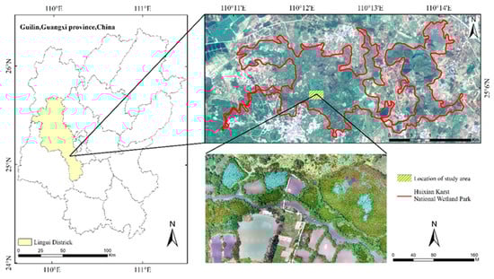
Figure 1.
Overview of the study area.
2.2. Data Source and Preprocessing
2.2.1. Acquisition of Field Survey and UAV Aerial Images
The UAV aerial images of this study were collected on 1 July 2021, when the vegetation in the Huixian wetland was flourishing, and the weather was clear and windless during the data collection period. The UAV model used in this study was DJI Phantom 4 Pro (DJI, Shenzhen, China), equipped with an OcuSync image transmission system as well as a 1-inch CMOS sensor (20 million effective pixels), and weighed about 1.4 kg [33]. The flight was planned and controlled in real time using a tablet equipped with DJI GS Pro software, with 80% heading overlap and 70% side overlap, and vertical downward aerial photography at a flight speed of 7 m/s. In order to obtain RGB images with different spatial resolutions, the UAV was flown at altitudes of 40, 60, 80, 100, 120, 140, 160, 180, and 200 m, respectively (Table 1). The flight mission was conducted under the permission of the relevant local management.

Table 1.
The spatial resolution and the number of aerial pieces corresponding to the flight height of the UAV.
2.2.2. UAV Aerial Image Processing
Firstly, POS data such as longitude and latitude coordinates and flight attitude of UAV aerial images were imported into Pix4D Mapper 4.4.12 software. Subsequently, an image quality check was carried out in order to remove fuzzy images with heading overlap rates of less than 80% and side overlap rates of less than 70%. Control points were inserted in order to correct geometric errors and to re-optimize the images. Afterward, the images were automatically matched through spatial triad solution and block adjustment in order to generate dense point cloud data. Finally, the dense point cloud data were utilized to construct a TIN triangulation network and to generate digital orthophoto maps (DOMs).
The mosaic of DOMs and the histogram matching homogenization process were completed in ENVI 5.3 software using the Seamless Mosaic tool. The images were then cropped in ArcGIS 10.6 in order to obtain nine aerial images (the spatial resolution of the Am were 1.2, 1.8, 2.4, 2.9, 3.6, 4.1, 4.7, 5.3, and 5.9 cm, respectively). In this study, the image with the highest resolution (1.2 cm) was resampled in order to examine the differences in the performance of wetland vegetation species and ground object identification between aerial images and resampled images. According to previous studies, in cases where an image was resampled using the nearest neighbor, bilinear, and cubic convolution methods, their smoothing and sharpening effects may significantly influence the final results [23]. Therefore, the pixel aggregate method was employed in order to reduce the spatial resolution of images, thereby generating eight corresponding resampled images (the spatial resolution of the An were 1.8, 2.4, 2.9, 3.6, 4.1, 4.7, 5.3, and 5.9 cm, respectively).
2.2.3. Reference Data
Based on the image with 1.2 cm spatial resolution and in addition to the field investigation results and the photographic record data, a detailed reference image of real vegetation species and ground objects (Figure 2) was obtained by employing the artificial vectorization method as a means for accuracy verification, and the acreage occupied by each vegetation species and ground objects within the study area was calculated (Table 2).
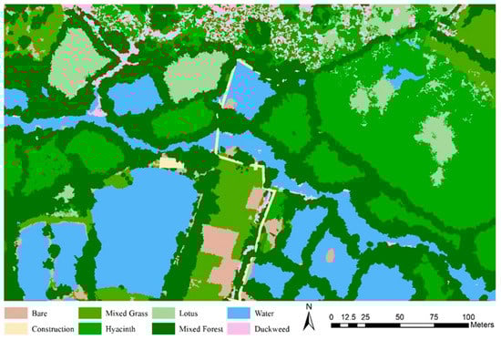
Figure 2.
Ground truth reference image.
Table 2.
The acreage occupied by each vegetation species and ground object in the study area.
2.3. Methods
Based on the Am and the An, GEOBIA was utilized in order to classify wetland vegetation species and ground objects within the study area (Figure 3). This procedure involved (1) selecting the appropriate scale parameter for multi-resolution segmentation through the ESP2 tool; (2) selecting and evaluating feature variables using the feature space optimization tool of the eCognition Developer 9.0 software and using the mean decreased accuracy (MDA) method of RF; (3) classifying vegetation species and ground objects from multi-scale images using four machine learning classifiers (RF, SVM, KNN, Bayes); (4) evaluating the accuracy of the classification results based on the overall accuracy, the Kappa coefficient, the producer accuracy, the user accuracy, and the average accuracy.
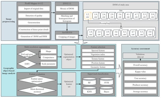
Figure 3.
Technical route of this study.
2.3.1. Preparation of Training Samples
The images generated through aerial photography by a UAV at 40 m altitude had a spatial resolution of 1.2 cm, in which it was possible to identify each vegetation species and ground object by means of visual interpretation. According to the results of the field survey and the differences between the characteristics of the UAV images, the vegetation species within the study area were divided into lotus, hyacinth, duckweed, mixed forest, and mixed grass, and the ground objects were divided into construction, water, and bare. In order to produce the training sample dataset, 103 randomly selected points were created in ArcGIS 10.6 software on 1.2 cm image layers across the study area (Figure 4) and each point was assigned a value (Table 3).
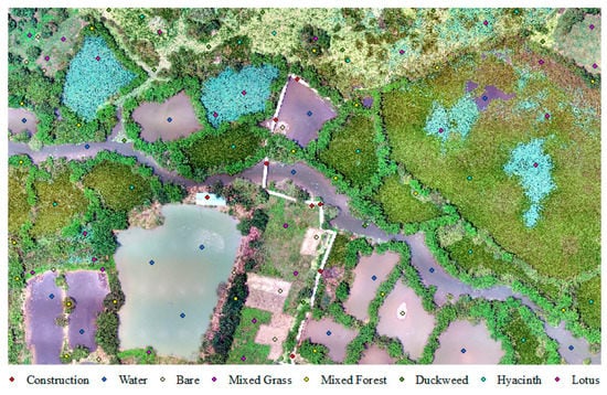
Figure 4.
Spatial distribution of training samples.
Table 3.
Training sample size in the study area.
2.3.2. Multi-Resolution Segmentation
GEOBIA is primarily based on image segmentation [34]. In this study, the fractal net evolution approach (FNEA) was employed for the segmentation of the Am and the An. This method belongs to a multi-resolution segmentation algorithm that merges bottom-up regions of pixels under the criterion of minimal heterogeneity in order to compose objects of different sizes. The segmented image objects were located relatively close to the natural boundaries of vegetation species and ground objects, and each image object contained spectral information, geometric information, texture information, and position information.
In the multi-resolution segmentation algorithm, the shape parameter is used to calculate the percentage of shape uniformity weighted relative to the spectral value, and the compactness parameter is a sub-parameter of shape, which is used to optimize the compactness of image objects. The sum of the weight of color and shape, smoothness and compactness is 1 [35]. With eCognition Developer 9.0 software, only the shape and compactness parameters are required to be manually configured, and the color and smoothness parameters are automatically generated.
Based on previous studies and subsequent experiments, the parameter values of shape and compactness were ultimately determined to be 0.2 and 0.5, respectively. Using the scale parameter (SP), it was possible to control the internal heterogeneity of detected objects, which was related to their average size; i.e., the larger the SP, the higher the internal heterogeneity, which increased the number of pixels per object, and vice versa. Due to the fact that SP is the most central parameter in multi-resolution segmentation algorithms and has the greatest impact on classification accuracy, thus it is crucial to determine the size of SP. The traditional method of calculating the size of SP is trial and error, which is highly contingent and time-consuming [36]. In this study, the ESP2 tool [37] was used to determine the optimal SP for multi-resolution segmentation. Since the initial value and step size in the ESP2 tool were not altered, the obtained results did not reach the peak value, but rather exhibited a smooth or steep curve. Therefore, it is essential to change the initial value and step size in ESP2. Table 4 shows the specific parameters that were determined after several experiments.
Table 4.
Parameters of the ESP2 tool.
2.3.3. Feature Selection and Evaluation
The second key step in GEOBIA is feature selection. Features that significantly influence the classification accuracy give the target object a high separability, i.e., the intra-class similarity is high, while the inter-class similarity is low. According to the image characteristics of the study area, five types of features were comprehensively considered on the basis of optimal segmentation, including spectral features, vegetation index [38,39], geometric features, position features, and texture features [40]. Furthermore, 90 feature variables were identified to form the initial feature space (Table 5), and the formula was presented for the calculation of each vegetation index (Table 6).
Table 5.
Object features.
Table 6.
Vegetation index and calculation formula.
Feature optimization is necessary for high-dimensional data, required to reduce data redundancy and enhance the model’s comprehension of features, thereby improving its generalization ability [41,42]. The feature space optimization tool in eCognition Developer 9.0 software was utilized to calculate a total of 90 feature variables, and the detailed information of the separability between all feature groups and classes was obtained. Taking the image with a spatial resolution of 1.2 cm as an example, it was evident that the separation distance between classes changed in accordance with the number of features (Figure 5). In the case where the feature dimension was 45, the separation distance between sample classes was the greatest (2.949).
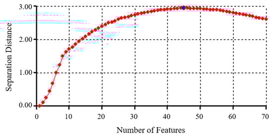
Figure 5.
The change in separability between the number of features and classes (1.2 cm spatial resolution image), and the blue diamond (indicating value 2.949) was the maximum separation distance.
Although some feature variables were selected after feature optimization, the remaining feature variables still exhibited a certain degree of correlation with one another. In this study, the mean decreased accuracy (MDA) method of RF was employed in order to further reduce the dimensions of the feature variables. The principle of the method is to reorder the original features, and then calculate the impact of sequence change on the model accuracy. In the case of certain unimportant feature variables, sequence changes have a minimal impact on the accuracy of the model; however, for certain key feature variables, sequence changes result in a reduction in the accuracy of the model [43,44]. Based on the results of MDA, all features were ranked from the largest to the smallest according to their degree of importance. Consequently, 20 to 30 features remained after the least significant features were removed. These features were put into RF, SVM, KNN, and Bayes models to identify wetland vegetation species and ground objects in the resulting UAV images.
2.3.4. Supervised Classification
The machine learning algorithm is a non-parametric supervision method, which has achieved remarkable success in the classification of remote sensing images in recent years [45]. The four classifiers used here were employed based on their effectiveness in previous studies; however, the performance of these algorithms is largely dependent on their own parameter values [46,47].
RF is an algorithm that integrates multiple trees through the approach of ensemble learning, and a “decision tree” serves as its basic unit. A forest is represented by many decision trees, and each tree yields a classification result, and the category with the greatest number of votes is designated as the classification result [48,49,50]. In this study, the RF classifier from the Scikit-Learn library of the Python platform was employed. Firstly, in order to estimate the overall classification effect, mtry was maintained at the default value, which was the square root of input feature variables, and then ntree was gradually increased from 100 to 150, 200, and 500. It was found that the classification effect was highest when ntree was set to 200. In the case where the value of ntree was set to 200, changing the value of mtry from the default value to a lower or higher value led to a reduction in the classification accuracy of the image. Accordingly, when the RF classifier was invoked in the Scikit-Learn library, mtry was required to be set as the default value, and ntree was required to be set to 200, which was most conducive to the identification of wetland vegetation species and ground objects in UAV images.
SVM is a machine learning algorithm derived from statistical learning theory developed by Vapnik’s team [51]. The prime feature of SVM is its ability to simultaneously minimize the empirical error and maximize the classification margin of images, i.e., supervised learning is accomplished by finding a hyperplane that can ensure both the accuracy of the classification and also maximize the margin between two types of data [52]. There are two types of kernels in SVM: the linear kernel and the radial basis function. In this work, we initially examined the impact of the radial basis function on the classification, and discovered that the accuracy of the classification result was insufficient. As a result, this study tested various penalty coefficients C using the linear kernel. Finally, it had been determined that in order to achieve the best classification effect, the value of C must be set to 5.
KNN is a commonly utilized nonlinear classifier in which the classification of an object depends on its neighboring samples [53]. Furthermore, if the majority of the object’s k nearest neighboring samples in the feature space belong to one particular class, then the sample is determined to belong to the same class as well [54]. Therefore, the k value is the key parameter of KNN. In this study, k values ranging from 1 to 10 were tested, and it was finally determined that the most accurate classification results could be obtained with the k value of 2.
Bayes is a simple probabilistic classification model based on Bayes’ theorem and assumes that features are not correlated with each other. The algorithm utilizes training samples as a means to estimate the mean vector and covariance matrix for each class and then incorporates them into the classification process [55]. It is not necessary to set any parameters for the Bayes classifier.
2.3.5. Accuracy Assessment
In this study, the overall accuracy (OA, Equation (1)) and Kappa coefficient were used as a means to evaluate the overall classification effects of wetlands on UAV images. OA represents the probability that the classification result is consistent with the actual ground object information. The Kappa coefficient (Equation (2)) is obtained through the statistical calculation of each element in the confusion matrix. The multivariate data analysis method was adopted, which takes into account the number of samples correctly classified by the model in addition to the “commission” and “omission” samples of the model, in order to accurately represent the degree to which the classification results match actual ground objects [56].
Producer accuracy (PA, Equation (3)), user accuracy (UA, Equation (4)), and average PA and UA (AA) were employed in order to discern the identification accuracy of wetland vegetation species and ground objects. PA refers to the percentage of pixels accurately classified in comparison with the number of pixels of the specific class in the reference data. UA refers to the percentage of pixels correctly classified in comparison with the number of all pixels classified into the same class [57].
In this study, each classifier (RF, SVM, KNN, Bayes) contained 9 the Am classification results and 8 the An classification results, which were compared using ground truth reference images covering the entire study area for the purpose of conducting a total of 68 accuracy evaluations.
where is the total number of evaluation data samples; is the number of samples of class in the classification result data and class in the validation data; is the sum of the class of the classification result; is the sum of class of the validation data.
3. Results
3.1. The Optimal SP of the Am and the An
Figure 6 showed the LV and ROC curves of the image with a spatial resolution of 1.2 cm. It was evident that the peak values of the curve were 323, 393, 453, 493, and 543. In cases where the SP was set as 453, 493, and 543, isolated and small vegetation species, such as lotus and hyacinth, led to incomplete segmentation results. In addition, various vegetation species may also be included in the same segmented object. The OA was 83.2, 82.4, and 80.1%, respectively, when we substituted the segmented objects into the RF classification model, and the classification results showed that the lotus or hyacinth was integrated into the adjacent large mixed forest. In the case where SP was set as 323, the segmented objects of large and uniform classes such as water, construction, and mixed forests led to the occurrence of over-segmentation, and the OA was 81.3%. In the classification results, other isolated and small vegetation species such as mixed grass, hyacinth, etc., appeared in areas that were originally all mixed forests. With the SP set to 393, it was possible to effectively segment all vegetation species and ground objects (Figure 7). The OA was 85.3%, and there were relatively few misclassifications in the classification results.
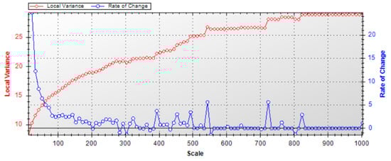
Figure 6.
Results of ESP2 scale analysis (1.2 cm spatial resolution image).
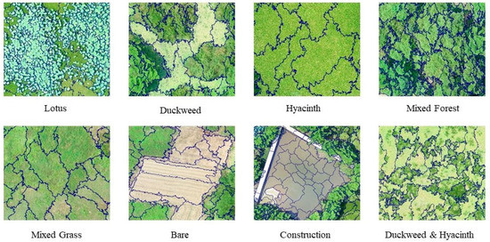
Figure 7.
Segmentation results of vegetation species and ground objects (1.2 cm spatial resolution image).
Images with different spatial scales corresponded to different optimal SPs (Figure 8), and as the spatial resolution decreased, the optimal SP of the image also decreased, as well as the required segmentation time. In cases where the spatial resolution exceeded 1.8 cm, the required SP set reached more than 300; moreover, the segmentation process took longer. In cases where the spatial resolution was in the range of 2.4~5.9 cm, it led to an SP setting of 90~200, with a relatively shorter segmentation time. Even at the same spatial resolution, there were some variations in the SP required for the Am and the An.
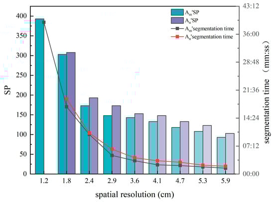
Figure 8.
The variation trend of the optimal SP and segmentation time in the Am and the An.
3.2. Feature Selection and Evaluation Results
3.2.1. The Importance of the Am Feature Variables
Among the Am, the importance of the feature variables was: vegetation index > position features > spectral features > texture features > geometric features (Figure 9). According to the importance evaluation, the red, blue, and EXG indices of the vegetation indices scored the highest. However, the importance of the three vegetation indices varied according to the scale of the images. In the information identification of ultra-high resolution images, X center and Y max were two of the most essential position features and also scored highly in the important evaluation of multi-scale images. In the case of the image with a spatial resolution of 1.2 cm, the X center was more crucial than the vegetation index, which was the most influential feature of the classification procedure. In the case of the 2.9 cm image, Y max served as the feature with the highest importance among the position features; subsequently, the importance of Y max gradually decreased in accordance with the decrease in the spatial resolution.
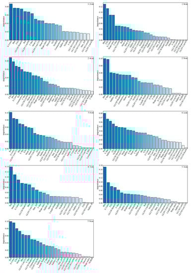
Figure 9.
Evaluation results of the importance of each feature in the Am.
Spectral features and texture features exhibited a different type of importance in the case of various images with varying spatial resolutions. In the case of multi-scale images, mean R, mean G, and stddev B were the most important spectral features for the classification procedure, and all exhibited a relatively high degree of importance in the Am. At a resolution of 2.9 cm, the importance of mean R exceeded that of mean G, and the distinction between the two became more obvious as the spatial resolution decreased. In the case of the 2.9 cm image, stddev B was the most important spectral feature and exhibited the most significant impact on the classification accuracy, whereas the importance of stddev B was relatively reduced in images above or below the same spatial resolution. The importance of stddev R gradually increased in accordance with the decrease in the spatial resolution. GLCM mean (0) was one of the most important texture features in the information identification procedure of ultra-high spatial resolution images; thus, it was essential in every dataset.
In multi-scale images, geometric features tended to be relatively less important. shape index and compactness were of minor importance in the case of images with spatial resolutions ranging from 1.8 to 2.9 cm, and the shape index was the most important geometric feature in the 1.8 cm image. With the decrease or increase of spatial resolution, the shape index gradually became less important.
3.2.2. The Importance of the An Feature Variables
Among the An, the importance of the feature variables was: vegetation index > position features > spectral features > texture features > geometric features (Figure 10), which was similar to the importance ranking of the feature variables in the case of the Am. In the case of the An, blue and EXG exhibited the highest degree of importance in the multi-scale images and had the most significant impact on the identification accuracy of wetland vegetation species and ground objects. Red was another vegetation index feature with a high degree of importance in the case of 1.8~3.6 cm images; however, it exhibited low importance in the case of 4.1~5.9 cm images. The position feature with the highest degree of importance in the multi-scale images was X center, followed by Y max. All other position features had little influence on the classification accuracy.
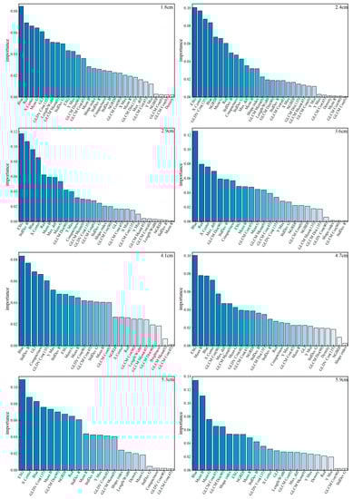
Figure 10.
Evaluation results of the importance of each feature in the An.
The importance of the spectral features was generally high for mean G, mean B, and stddev B. Stddev B became more important as the spatial resolution decreased, and then slightly decreased with fluctuations, reaching its maximum importance in the 2.9 cm images. The importance of mean B in the 1.8~4.1 cm spatial resolution images was not very significant; however, it exhibited a very high degree of importance in the case of 4.7~5.9 cm spatial resolution images. In the case of 1.8~3.6 cm images, the importance of max_diff gradually increased in accordance with the decrease in the spatial resolution. Thus, max_diff became the most important spectral feature in the case of 3.6 cm images. The texture features with a generally high degree of importance in the An were GLDV contrast (135), GLCM dissimilarity (90), and GLCM mean (0). The importance of GLCM correlation (90) was only significant in the case of the 4.7 cm image, and it exhibited a minor degree of importance in the case of images with other scales.
Geometric features were less important in the An. In the case of 2.4~4.7 cm images, compactness was the geometric feature with the highest degree of importance. However, the shape index exhibited a higher degree of importance in geometric features and exceeded compactness in the case of the 5.3~5.9 cm images.
3.3. Overall Classification Accuracy
3.3.1. Overall Classification Accuracy of the Am
In the Am, the OA and Kappa coefficients increased and then decreased in accordance with the decrease in the spatial resolution, peaking at the resolution of 2.9 cm (Table 7). The OA and kappa coefficients of the Am classification results indicated the same pattern of change in the different classifiers. In the case of the resolution interval ranging from 1.2 to 2.9 cm, the results of the OA of RF, SVM, and KNN were comparable (ranging from 85.2 to 88.8%) and were greater than the OA of Bayes. In the case of the resolution interval ranging from 3.6 to 5.9 cm, the performance of SVM was superior to that of RF, and the gap between the quality of their results became larger as the spatial resolution decreased. At spatial resolutions below 2.9 cm, KNN’s classification accuracy decreased sharply, while it fell below that of Bayes at 5.3 cm.
Table 7.
Overall classification accuracy of each classifier in the Am.
3.3.2. Overall Classification Accuracy of the An
The variation tendency of OA and kappa of the four classifiers in the An was basically the same as that in the Am, and both of them peaked at 2.9 cm resolution (Table 8). As a whole, the performance of the RF classifier was the best. In the resolution range of 1.2~2.4cm, the accuracy of KNN was higher than that of SVM, but with the decrease of spatial resolution, that is, in the resolution range of 2.9~5.9cm, the accuracy of SVM was higher than that of KNN, and the variation tended to be flat.
Table 8.
Overall classification accuracy of each classifier in the An.
3.4. Identification Accuracy of Vegetation Species and Ground Objects
Given the overall superiority of the RF classifier over SVM, KNN, and Bayes, the classification results of vegetation species and ground objects under the RF classifier were plotted in this study. The identification accuracy of vegetation species and ground objects was evaluated by PA, UA, and AA.
3.4.1. Identification Accuracy of Vegetation Species and Ground Objects in the Am
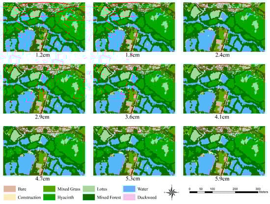
Disparities between the Am classification results and the ground truth reference image were most pronounced in the northern, north-eastern, and southern parts of the study area and are marked in red in Figure 11. In the multi-scale images, hyacinth, duckweed, and lotus in the northern part of the study area, were more likely to exhibit commission or omission. In the case of 4.7~5.9 cm images, mixed grass in the northeastern part of the study area was often incorrectly classified as hyacinth. In the case of the images with the resolutions of 1.2, 1.8, and 3.6~5.9 cm, a large amount of mixed grass in the southern part of the study area was incorrectly classified as mixed forest. In the Am, the classification results of water and construction were relatively consistent with the ground truth reference image. The spatial scale effect of the Am in the classification was analyzed by employing PA, UA, and AA.
In the Am, changes in spatial resolution had no significant effect on the identification of water. Moreover, the PA, UA, and AA of water were the highest (approximately 95%) in multi-scale images. In the case of hyacinth, mixed forest, and construction, the PA of the 1.2~2.9 cm images was very close at 86, 91, and 90%, respectively, and then the PA gradually decreased in accordance with the decrease in the spatial resolution. As a result of the change in the spatial resolution, PA exhibited a similar pattern for lotus and bare areas. PA initially increased and then gradually began to decline, peaking at 88.1 and 82.6%, respectively, in the 1.8 cm image. In the case of mixed grass and duckweed, PA results varied greatly depending on the different resolutions. Duckweed exhibited the highest PA in 2.4 and 2.9 cm images. In the multi-scale images, the UA of lotus, hyacinth, mixed forest, and construction was close and decreased gradually in accordance with the decrease in the spatial resolution. As compared with other classes, the UA of duckweed was the lowest in all the multi-scale images. The highest AA for lotus, hyacinth, and bare was in the 1.8 cm image, while the highest AA for mixed forest, mixed grass, and duckweed was in the 2.4 and 2.9 cm images (Figure 12).
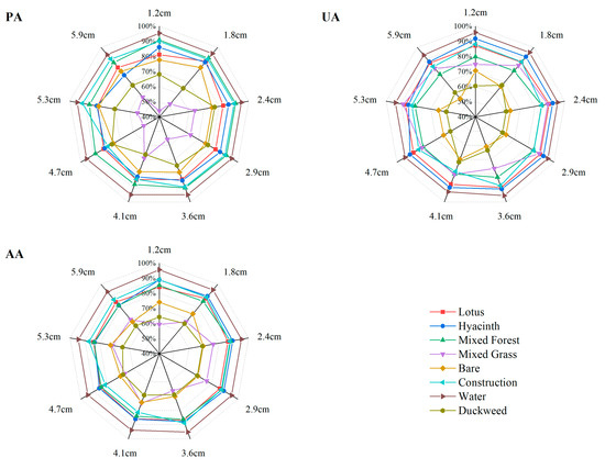
Figure 12.
Identification accuracy of vegetation species and ground objects in the Am.
3.4.2. Identification Accuracy of Vegetation Species and Ground Objects in the An
The disparities between the An classification results and ground truth reference images were most pronounced in the northern and north-eastern parts of the study area and are marked in red in Figure 13. In the An classification results, hyacinth, duckweed, lotus, and mixed forests in the northern part of the study area were more likely to exhibit commission or omission, and mixed grass in the north-eastern part was also more likely to be incorrectly classified as mixed forest. Similar to the Am classification results, in the case of the An results, the classification results of water and construction were relatively consistent with the ground truth reference images.
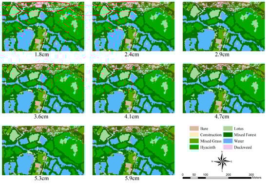
The PA, UA, and AA of water in the An results exhibited the highest accuracy in the multi-scale images (Figure 14). The PA of lotus, mixed forest, bare, and duckweed was significantly affected by the spatial resolution, in turn, the PA increased and then decreased in accordance with the decrease in the spatial resolution, peaking in the 2.9 cm image. In the multi-scale images, the PA of mixed grass was the lowest as compared to other classes. In addition, the UA of lotus, hyacinth, and mixed grass also exhibited similar spatial scale effects. The UA first increased and subsequently declined in response to the decrease in the spatial resolution, peaking in the 2.9 cm image. Overall, the UA of hyacinth was the highest, followed by that of lotus and mixed grass. The AA of lotus, hyacinth, duckweed, mixed forest, bare, construction, and water showed an analogous pattern of change under the influence of different spatial resolutions. The AA increased gradually in the resolution range of 1.8~2.9 cm and decreased gradually in the resolution range of 2.9~5.9 cm.
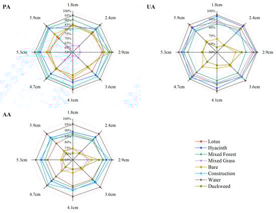
Figure 14.
Identification accuracy of vegetation species and ground objects in the An results.
4. Discussion
As an effective tool for the classification of remote sensing images, GEOBIA has been widely used in the classification of wetland vegetation species and ground objects [58]. In using GEOBIA, image segmentation is the first key step. Previous studies have shown that the FNEA multi-resolution segmentation algorithm is one of the most popular image segmentation algorithms used for the identification of wetland vegetation species and ground objects. Appropriate segmentation parameters directly impact the patch size of the generated object as well as the extraction accuracy of actual vegetation species and ground objects. Therefore, it is crucial to determine the optimal segmentation parameter value for the identification of wetland vegetation species and ground objects [32]. The FNEA multi-resolution segmentation technology utilized three main parameters: shape, compactness, and SP. Changes in the SP had a greater impact on the quality of segmentation results than changes in the shape and compactness [59]. In this study, after determining the shape and compactness parameters of 0.2 and 0.5, respectively, through trial and error, the SP was selected by the ESP2 tool in order to overcome the subjective influence of human perception on the results. However, the current research on the optimal SP is only for a specific spatial resolution image, and there are still some deficiencies in the research on the response of aerial images and resampled images with different spatial resolutions. The results of this study demonstrated that a higher spatial resolution corresponded to a longer segmentation time as well as a greater optimal SP value (Figure 8). This was because higher spatial resolutions resulted in larger amounts of data and longer computer processing times for images. Thus, it is imperative that the effectiveness of image processing be taken into account in future studies instead of excessively focusing on spatial resolution while gathering UAV aerial images. Even at the same spatial resolution, the optimal SP value for the An was somewhat bigger than that for the Am. In light of the fact that the internal heterogeneity of the image in the An was lower as a result of resampling, an increase in the SP value was capable of producing segmentation results that were comparable to those of the Am. As a result of the combination of the ideal segmentation parameters, all types of vegetation species and ground objects were separated, and each object within an image was relatively close to the natural boundaries of vegetation species and ground objects, which was acceptable for further processing.
In GEOBIA, feature selection is the second key step after image segmentation. Due to the limited spectral resolution of UAV-RGB images and the serious confusion of the spectra of various wetland vegetation species, this study employed vegetation indexes, texture features, position features, and geometric features as a means to compensate for the lack of spectral information. However, having too many feature variables might cause data redundancy and overfitting, which leads to a reduction in the classification accuracy of the results. Therefore, this study used the feature space optimization tool in addition to the MDA method for feature optimization in order to improve the processing efficiency of high-dimensional data and to calculate the importance of each feature variable. As demonstrated in previous research, the importance of the vegetation index was highest, while the importance of the geometric features was lowest [41,60]. However, a sizeable portion of the important evaluation in this study was accounted for by position features, specifically X center and Y max. It was possible that this was due to the geographically constrained nature of the research area selected for this study, which magnified the significance of X center and Y max. In other words, the addition of X center and Y max was more conducive to improving the classification accuracy when classifying wetlands in small areas. The importance of each geometric feature was generally low. Thus, geometric features cannot be arbitrarily added in future studies. When comparing the importance of each vegetation index and texture feature between the Am and the An, red, blue, EXG, and GLCM mean (0) were found to have relatively high importance, suggesting that when classifying wetland vegetation species and ground objects, these feature variables should be taken into consideration first. The results showed that there were significant differences between the importance of some feature variables between the Am and the An, and the max_diff feature in the An was more important than the Am in spectral features. Moreover, the results also indicated that the GLDV contrast (135), GLCM dissimilarity (90), and GLCM correlation (90) feature in the An were more important than the Am in texture features, which was possibly one of the reasons for the higher classification accuracy of the An than the Am in the final classification results.
RF, SVM, KNN, and Bayes are machine learning classifiers commonly utilized for image classification, and this study evaluated the performance of these classifiers in the classification of wetland vegetation species and ground objects by OA and kappa coefficients. As demonstrated in previous research results, different classifiers functioned differently, with RF classifiers generally performing the best [55]. Accordingly, the classification of wetland vegetation species and ground objects should prioritize RF classifiers in future research. This study focused on exploring the responses of these four classifiers to the spatial resolution of images, and the results indicated that the trends of OA and kappa coefficients in the Am and the An were relatively the same in the cases of various classifiers. In the case where the spatial resolution was lower than 2.9 cm, the OA and kappa coefficients decreased significantly (Table 7 and Table 8), which was due to the increasing number of mixed pixels caused by the decreasing spatial resolution. A pixel might contain information of multiple classes, and the classification result of the pixel was related to the proportion of classes in the mixed pixel. Small and fragmented classes were easily replaced by other large and uniform classes. The edges of the patches were more prone to increase commission errors or omission errors [61]. However, a higher spatial resolution did not necessarily mean a better image [24]. For example, the classification accuracy of 1.2, 1.8, and 2.4 cm images was lower than that of 2.9 cm images, because wetland vegetation species and ground objects had specific physical sizes, and spatial resolution above a certain threshold was not conducive to the identification of vegetation species and ground objects [62,63]. Although providing detailed information regarding vegetation species and ground objects, ultra-high spatial resolution images were obviously harmful in enhancing the phenomenon of different spectra of the same vegetation species or ground objects. Consequently, this also increased the difficulty of identifying vegetation species and ground objects. In addition, the ultra-high spatial resolution caused multiple super-impositions of information, which greatly reduced the processing efficiency of the images [62,64]. In future research, it is unnecessary to relentlessly strive for a spatial resolution that is better than the threshold value, and the flight altitude of UAVs may also improve the operational efficiency by covering a larger area, thus ensuring the maximum classification accuracy. It was also shown that the overall classification accuracy of the An was higher than that of the Am, probably because the images obtained by pixel aggregation resampling contained fewer disparities in spectral and textural features among homogeneous vegetation species or ground objects and more disparities in spectral and textural features among heterogeneous vegetation species or ground objects as compared with the corresponding aerial images [20,65]. Resampled images were therefore more useful for identifying wetland vegetation species and ground objects in the spatial resolution range of 1.2~5.9 cm than aerial images.
Based on the RF classifier, the spatial scale effects of each vegetation species and ground object in classification were explored, which has a good reference for selecting the best resolution image to identify wetland vegetation species and ground objects. In this study, the UA, PA, and AA of the RF classifier were calculated for each vegetation species and ground object in the Am and the An (Figure 12 and Figure 14), and the results indicated that water exhibited an accurate and stable identification accuracy in the Am and the An, which may be due to the lesser degree of heterogeneity among water objects formed after multi-resolution segmentation by FNEA. Moreover, water objects differed significantly from other objects, resulting in an easier extraction of water in wetland ecosystems. Figure 12 demonstrated that higher spatial resolution and more informative images, such as the 1.2~2.9 cm images, were needed if the PA of hyacinth, mixed forest, and construction was to be improved in the Am. The UA of duckweed was significantly lower than that of other classes in the Am, which was caused by the fact that duckweed was primarily distributed in the northern part of the study area, where the vegetation species were highly fragmented. Moreover, duckweed was heavily mixed with hyacinth, and the duckweed parcels had irregular shape and size in the multi-scale images, resulting in the level of identification accuracy for duckweed being the lowest. In the An, mixed grass exhibited the lowest PA, and mixed forest exhibited a higher PA. Because mixed grass tended to form mixed pixels with the surrounding edge areas of mixed forest, mixed grass was easily incorrectly classified as mixed forest, thus, reducing the identification accuracy of mixed grass. In addition, the optimal spatial resolution required for the extraction of certain vegetation species or ground objects varied in the case of the Am and the An. In the Am, some vegetation species and ground objects (e.g., lotus, hyacinth, and bare) exhibited the highest AA in the 1.8 cm image, and some vegetation species (such as mixed forest, mixed grass, and duckweed) exhibited the highest AA in the 2.4 and 2.9 cm images. The AA of most vegetation species and ground objects changed regularly in the An as a result of the influence of the spatial resolution, which was possible because the An was resampled from a single image by pixel aggregation and the imaging mechanism of each scale was quite similar. In contrast, the Am was acquired by UAV flight at various altitudes in the field, which was easily affected by wind speed, light, and other disturbing factors during flight, resulting in some variability in image information at different scales. In the An, the 1.8~2.4 cm images with detailed characteristics also induced noise in the identification procedure of wetland vegetation species and ground objects, while the image element mixing phenomenon was common in the 3.6~5.9 cm images, which meant it was not possible to accurately distinguish wetland vegetation species or ground objects. The 2.9 cm image in the An was therefore less noisy and suitable enough for the purpose of distinguishing vegetation species and ground objects from the diverse wetland environment. In future studies, the designation of images with optimal spatial resolutions is crucial to obtain the ideal classification results for vegetation species and ground objects.
5. Conclusions
In this study, the UAVs were flown at different altitudes around the study area in order to obtain aerial images (Am) with different spatial resolutions, and then the aerial image with a spatial resolution of 1.2 cm was resampled by pixel aggregation in order to generate resampled images (An) corresponding to the spatial resolution of the Am. In the GEOBA method, various machine learning classifiers were employed to classify the vegetation species and ground objects of the Am and the An, based on the ideal segmentation results and feature selection. The following conclusions were drawn from this study:
- (1)
- In the image segmentation step of GEOBIA, SP is the most critical parameter in the multi-resolution segmentation algorithm. It is important to select optimal SP for images with different spatial resolutions in order to segment each vegetation species and ground object. In this study, the optimal SP to be set for the resampled image was larger than that for the aerial image at the same spatial resolution. The optimal SP progressively declined in accordance with the decrease in the spatial resolution and also resulted in a significant decline in the required segmentation time.
- (2)
- In the feature selection step of GEOBIA, different feature variables are required for different spatial resolution images. Aerial images and resampled images differ in their spectral or texture information due to differences in imaging mechanisms. For example, in this study, the importance of some spectral features and texture features in the An was higher than that in the Am. The importance of each feature variable in the Am and the An was as follows: vegetation index > position feature > spectral feature > texture feature > geometric feature. Therefore, it is necessary to select appropriate feature variables for images with different spatial resolutions and different imaging mechanisms to assure classification accuracy in future studies.
- (3)
- The resampled images typically had better classification accuracy than the aerial images in the spatial resolution range of 1.2~5.9cm. Moreover, in terms of total classification accuracy, the RF classifier was more precise, outperforming the SVM, KNN, and Bayes classifiers. When the spatial resolution fell below a certain threshold, some small and fragmented classes were susceptible to misclassification because of the mixed pixel effect. The most adequate resolution was achieved when the spectrum or texture exhibited the smallest intra-class variance as well as the largest inter-class variance.
- (4)
- For the same vegetation species or ground object, the PA, UA, and AA were different when using different spatial resolution images for classification. In order to achieve a higher classification accuracy during UAV flight experiments and data processing, it is crucial to choose appropriate spatial resolution images based on the distribution characteristics and patch size of each vegetation species and ground object in a certain study area. It is noteworthy that the optimal spatial resolution required for the same vegetation species or ground objects differed between aerial images and resampled images. For instance, in this study, in the Am, the highest extraction accuracy of lotus and hyacinth was in the 1.8 cm image, and the highest extraction accuracy of duckweed was in the 2.3 and 2.9 cm images, while in the An, the 2.9 cm image was the most favorable for the identification of lotus, hyacinth, and duckweed.
Author Contributions
Conceptualization, J.C. and Z.C.; methodology, J.C. and Z.C.; validation, J.C. and Z.C.; formal analysis, J.C. and Z.C.; resources, J.C., Z.C. and R.H.; software, Z.C. and R.H.; writing—original draft preparation, Z.C.; writing—review and editing, J.C. and Z.C.; visualization, J.C. and H.Y.; supervision, J.C, X.H., and T.Y.; funding acquisition, J.C. and G.Z. All authors have read and agreed to the published version of the manuscript.
Funding
This study was supported by grants from Guangxi Science and Technology Base and Talent Project (GuikeAD19245032), Major Special Projects of High Resolution Earth Observation System (84-Y50G25-9001-22/23), the National Natural Science Foundation of China (41801030, 41861016), Guangxi Key Laboratory of Spatial Information and Geomatics (19-050-11-22), and Research Foundation of Guilin University of Technology (GUTQDJJ2017069).
Data Availability Statement
Not applicable.
Conflicts of Interest
The authors declare no conflict of interest.
References
- Wang, Z.; Wu, J.; Madden, M.; Mao, D. China’s Wetlands: Conservation plans and policy impacts. Ambio 2012, 41, 782–786. [Google Scholar] [CrossRef] [PubMed]
- Yang, Y.; Chen, J.; Lan, Y.; Zhou, G.; You, H.; Han, X.; Wang, Y.; Shi, X. Landscape Pattern and Ecological Risk Assessment in Guangxi Based on Land Use Change. Int. J. Env. Res. Public Health 2022, 19, 1595. [Google Scholar] [CrossRef]
- Davidson, N.C. How much wetland has the world lost? Long-term and recent trends in global wetland area. Mar. Freshw. Res. 2014, 65, 934–941. [Google Scholar] [CrossRef]
- Koch, M.; Schmid, T.; Reyes, M.; Gumuzzio, J. Evaluating Full Polarimetric C- and L-Band Data for Mapping Wetland Conditions in a Semi-Arid Environment in Central Spain. IEEE J. Sel. Top. Appl. Earth Obs. Remote Sens. 2012, 5, 1033–1044. [Google Scholar] [CrossRef]
- Fu, B.; Zuo, P.; Liu, M.; Lan, G.; He, H. Classifying vegetation communities karst wetland synergistic use of image fusion and object-based machine learning algorithm with Jilin-1 and UAV multispectral images. Ecol. Indic. 2022, 140, 108989. [Google Scholar] [CrossRef]
- Davidson, N.C.; Fluet-Chouinard, E.; Finlayson, C.M. Global extent and distribution of wetlands: Trends and issues. Mar. Freshw. Res. 2018, 69, 620–627. [Google Scholar] [CrossRef]
- Dronova, I. Object-Based Image Analysis in Wetland Research: A Review. Remote Sens. 2015, 7, 6380–6413. [Google Scholar] [CrossRef]
- Adam, E.; Mutanga, O.; Rugege, D. Multispectral and hyperspectral remote sensing for identification and mapping of wetland vegetation: A review. Wetl. Ecol. Manag. 2009, 18, 281–296. [Google Scholar] [CrossRef]
- Guo, M.; Li, J.; Sheng, C.; Xu, J.; Wu, L. A Review of Wetland Remote Sensing. Sensors 2017, 17, 777. [Google Scholar] [CrossRef]
- Tana, G.; Letu, H.; Cheng, Z.; Tateishi, R. Wetlands Mapping in North America by Decision Rule Classification Using MODIS and Ancillary Data. IEEE J. Sel. Top. Appl. Earth Obs. Remote Sens. 2013, 6, 2391–2401. [Google Scholar] [CrossRef]
- McCarthy, M.J.; Merton, E.J.; Muller-Karger, F.E. Improved coastal wetland mapping using very-high 2-meter spatial resolution imagery. Int. J. Appl. Earth Obs. Geoinf. 2015, 40, 11–18. [Google Scholar] [CrossRef]
- Chen, Y.; He, X.; Xu, J.; Zhang, R.; Lu, Y. Scattering Feature Set Optimization and Polarimetric SAR Classification Using Object-Oriented RF-SFS Algorithm in Coastal Wetlands. Remote Sens. 2020, 12, 407. [Google Scholar] [CrossRef]
- Chen; Zhao; Zhang; Qin; Yi. Evaluation of the Accuracy of the Field Quadrat Survey of Alpine Grassland Fractional Vegetation Cover Based on the Satellite Remote Sensing Pixel Scale. ISPRS Int. J. Geo-Inf. 2019, 8, 497. [Google Scholar] [CrossRef]
- Chen, J.; Yi, S.; Qin, Y.; Wang, X. Improving estimates of fractional vegetation cover based on UAV in alpine grassland on the Qinghai–Tibetan Plateau. Int. J. Remote Sens. 2016, 37, 1922–1936. [Google Scholar] [CrossRef]
- Chen, J.; Huang, R.; Yang, Y.; Feng, Z.; You, H.; Han, X.; Yi, S.; Qin, Y.; Wang, Z.; Zhou, G. Multi-Scale Validation and Uncertainty Analysis of GEOV3 and MuSyQ FVC Products: A Case Study of an Alpine Grassland Ecosystem. Remote Sens. 2022, 14, 5800. [Google Scholar] [CrossRef]
- Arif, M.S.M.; Gülch, E.; Tuhtan, J.A.; Thumser, P.; Haas, C. An investigation of image processing techniques for substrate classification based on dominant grain size using RGB images from UAV. Int. J. Remote Sens. 2016, 38, 2639–2661. [Google Scholar] [CrossRef]
- Rominger, K.; Meyer, S. Application of UAV-Based Methodology for Census of an Endangered Plant Species in a Fragile Habitat. Remote Sens. 2019, 11, 719. [Google Scholar] [CrossRef]
- Sankey, J.B.; Sankey, T.T.; Li, J.; Ravi, S.; Wang, G.; Caster, J.; Kasprak, A. Quantifying plant-soil-nutrient dynamics in rangelands: Fusion of UAV hyperspectral-LiDAR, UAV multispectral-photogrammetry, and ground-based LiDAR-digital photography in a shrub-encroached desert grassland. Remote Sens. Environ. 2021, 253, 112223. [Google Scholar] [CrossRef]
- Yan, G.; Li, L.; Coy, A.; Mu, X.; Chen, S.; Xie, D.; Zhang, W.; Shen, Q.; Zhou, H. Improving the estimation of fractional vegetation cover from UAV RGB imagery by colour unmixing. ISPRS J. Photogramm. Remote Sens. 2019, 158, 23–34. [Google Scholar] [CrossRef]
- Roth, K.L.; Roberts, D.A.; Dennison, P.E.; Peterson, S.H.; Alonzo, M. The impact of spatial resolution on the classification of plant species and functional types within imaging spectrometer data. Remote Sens. Environ. 2015, 171, 45–57. [Google Scholar] [CrossRef]
- Meddens, A.J.H.; Hicke, J.A.; Vierling, L.A. Evaluating the potential of multispectral imagery to map multiple stages of tree mortality. Remote Sens. Environ. 2011, 115, 1632–1642. [Google Scholar] [CrossRef]
- Hu, P.; Guo, W.; Chapman, S.C.; Guo, Y.; Zheng, B. Pixel size of aerial imagery constrains the applications of unmanned aerial vehicle in crop breeding. ISPRS J. Photogramm. Remote Sens. 2019, 154, 1–9. [Google Scholar] [CrossRef]
- Liu, M.; Yu, T.; Gu, X.; Sun, Z.; Yang, J.; Zhang, Z.; Mi, X.; Cao, W.; Li, J. The Impact of Spatial Resolution on the Classification of Vegetation Types in Highly Fragmented Planting Areas Based on Unmanned Aerial Vehicle Hyperspectral Images. Remote Sens. 2020, 12, 146. [Google Scholar] [CrossRef]
- Lu, B.; He, Y. Optimal spatial resolution of Unmanned Aerial Vehicle (UAV)-acquired imagery for species classification in a heterogeneous grassland ecosystem. GIScience Remote Sens. 2017, 55, 205–220. [Google Scholar] [CrossRef]
- Narayanan, R.M.; Desetty, M.K.; Reichenbach, S.E. Effect of spatial resolution on information content characterization in remote sensing imagery based on classification accuracy. Int. J. Remote Sens. 2010, 23, 537–553. [Google Scholar] [CrossRef]
- Fu, B.; Wang, Y.; Campbell, A.; Li, Y.; Zhang, B.; Yin, S.; Xing, Z.; Jin, X. Comparison of object-based and pixel-based Random Forest algorithm for wetland vegetation mapping using high spatial resolution GF-1 and SAR data. Ecol. Indic. 2017, 73, 105–117. [Google Scholar] [CrossRef]
- Mahdavi, S.; Salehi, B.; Amani, M.; Granger, J.E.; Brisco, B.; Huang, W.; Hanson, A. Object-Based Classification of Wetlands in Newfoundland and Labrador Using Multi-Temporal PolSAR Data. Can. J. Remote Sens. 2017, 43, 432–450. [Google Scholar] [CrossRef]
- De Luca, G.; Silva, J.M.N.; Cerasoli, S.; Araújo, J.; Campos, J.; Di Fazio, S.; Modica, G. Object-Based Land Cover Classification of Cork Oak Woodlands using UAV Imagery and Orfeo ToolBox. Remote Sens. 2019, 11, 1238. [Google Scholar] [CrossRef]
- Duro, D.C.; Franklin, S.E.; Dubé, M.G. A comparison of pixel-based and object-based image analysis with selected machine learning algorithms for the classification of agricultural landscapes using SPOT-5 HRG imagery. Remote Sens. Environ. 2012, 118, 259–272. [Google Scholar] [CrossRef]
- Pande-Chhetri, R.; Abd-Elrahman, A.; Liu, T.; Morton, J.; Wilhelm, V.L. Object-based classification of wetland vegetation using very high-resolution unmanned air system imagery. Eur. J. Remote Sens. 2017, 50, 564–576. [Google Scholar] [CrossRef]
- Geng, R.; Jin, S.; Fu, B.; Wang, B. Object-Based Wetland Classification Using Multi-Feature Combination of Ultra-High Spatial Resolution Multispectral Images. Can. J. Remote Sens. 2021, 46, 784–802. [Google Scholar] [CrossRef]
- Fu, B.; Liu, M.; He, H.; Lan, F.; He, X.; Liu, L.; Huang, L.; Fan, D.; Zhao, M.; Jia, Z. Comparison of optimized object-based RF-DT algorithm and SegNet algorithm for classifying Karst wetland vegetation communities using ultra-high spatial resolution UAV data. Int. J. Appl. Earth Obs. Geoinf. 2021, 104, 102553. [Google Scholar] [CrossRef]
- Phantom 4 Pro/Pro_Plus Series User Manual CHS. Available online: https://dl.djicdn.com/downloads/phantom_4_pro/20211129/UM/Phantom_4_Pro_Pro_Plus_Series_User_Manual_CHS.pdf (accessed on 1 July 2022).
- Cao, J.; Leng, W.; Liu, K.; Liu, L.; He, Z.; Zhu, Y. Object-Based Mangrove Species Classification Using Unmanned Aerial Vehicle Hyperspectral Images and Digital Surface Models. Remote Sens. 2018, 10, 89. [Google Scholar] [CrossRef]
- Akar, A.; Gökalp, E.; Akar, Ö.; Yılmaz, V. Improving classification accuracy of spectrally similar land covers in the rangeland and plateau areas with a combination of WorldView-2 and UAV images. Geocarto Int. 2016, 32, 990–1003. [Google Scholar] [CrossRef]
- Qian, Y.; Zhou, W.; Yan, J.; Li, W.; Han, L. Comparing Machine Learning Classifiers for Object-Based Land Cover Classification Using Very High Resolution Imagery. Remote Sens. 2014, 7, 153–168. [Google Scholar] [CrossRef]
- Drǎguţ, L.; Tiede, D.; Levick, S.R. ESP: A tool to estimate scale parameter for multiresolution image segmentation of remotely sensed data. Int. J. Geogr. Inf. Sci. 2010, 24, 859–871. [Google Scholar] [CrossRef]
- Michez, A.; Piegay, H.; Lisein, J.; Claessens, H.; Lejeune, P. Classification of riparian forest species and health condition using multi-temporal and hyperspatial imagery from unmanned aerial system. Env. Monit. Assess. 2016, 188, 146. [Google Scholar] [CrossRef]
- Meyer, G.E.; Neto, J.C. Verification of color vegetation indices for automated crop imaging applications. Comput. Electron. Agric. 2008, 63, 282–293. [Google Scholar] [CrossRef]
- Lu, B.; He, Y. Species classification using Unmanned Aerial Vehicle (UAV)-acquired high spatial resolution imagery in a heterogeneous grassland. ISPRS J. Photogramm. Remote Sens. 2017, 128, 73–85. [Google Scholar] [CrossRef]
- Lou, P.; Fu, B.; He, H.; Li, Y.; Tang, T.; Lin, X.; Fan, D.; Gao, E. An Optimized Object-Based Random Forest Algorithm for Marsh Vegetation Mapping Using High-Spatial-Resolution GF-1 and ZY-3 Data. Remote Sens. 2020, 12, 1270. [Google Scholar] [CrossRef]
- Ebrahimi-Khusfi, Z.; Nafarzadegan, A.R.; Dargahian, F. Predicting the number of dusty days around the desert wetlands in southeastern Iran using feature selection and machine learning techniques. Ecol. Indic. 2021, 125, 107499. [Google Scholar] [CrossRef]
- Grabska, E.; Hostert, P.; Pflugmacher, D.; Ostapowicz, K. Forest Stand Species Mapping Using the Sentinel-2 Time Series. Remote Sens. 2019, 11, 1197. [Google Scholar] [CrossRef]
- Dobrinić, D.; Gašparović, M.; Medak, D. Sentinel-1 and 2 Time-Series for Vegetation Mapping Using Random Forest Classification: A Case Study of Northern Croatia. Remote Sens. 2021, 13, 2321. [Google Scholar] [CrossRef]
- Pham, L.T.H.; Brabyn, L. Monitoring mangrove biomass change in Vietnam using SPOT images and an object-based approach combined with machine learning algorithms. ISPRS J. Photogramm. Remote Sens. 2017, 128, 86–97. [Google Scholar] [CrossRef]
- Pasquarella, V.J.; Holden, C.E.; Woodcock, C.E. Improved mapping of forest type using spectral-temporal Landsat features. Remote Sens. Environ. 2018, 210, 193–207. [Google Scholar] [CrossRef]
- Sun, C.; Li, J.; Liu, Y.; Liu, Y.; Liu, R. Plant species classification in salt marshes using phenological parameters derived from Sentinel-2 pixel-differential time-series. Remote Sens. Environ. 2021, 256, 112320. [Google Scholar] [CrossRef]
- Adugna, T.; Xu, W.; Fan, J. Comparison of Random Forest and Support Vector Machine Classifiers for Regional Land Cover Mapping Using Coarse Resolution FY-3C Images. Remote Sens. 2022, 14, 574. [Google Scholar] [CrossRef]
- Belgiu, M.; Drăguţ, L. Random forest in remote sensing: A review of applications and future directions. ISPRS J. Photogramm. Remote Sens. 2016, 114, 24–31. [Google Scholar] [CrossRef]
- Millard, K.; Richardson, M. On the Importance of Training Data Sample Selection in Random Forest Image Classification: A Case Study in Peatland Ecosystem Mapping. Remote Sens. 2015, 7, 8489–8515. [Google Scholar] [CrossRef]
- Mohammadimanesh, F.; Salehi, B.; Mahdianpari, M.; Motagh, M.; Brisco, B. An efficient feature optimization for wetland mapping by synergistic use of SAR intensity, interferometry, and polarimetry data. Int. J. Appl. Earth Obs. Geoinf. 2018, 73, 450–462. [Google Scholar] [CrossRef]
- Chabalala, Y.; Adam, E.; Ali, K.A. Machine Learning Classification of Fused Sentinel-1 and Sentinel-2 Image Data towards Mapping Fruit Plantations in Highly Heterogenous Landscapes. Remote Sens. 2022, 14, 2621. [Google Scholar] [CrossRef]
- Martínez Prentice, R.; Villoslada Peciña, M.; Ward, R.D.; Bergamo, T.F.; Joyce, C.B.; Sepp, K. Machine Learning Classification and Accuracy Assessment from High-Resolution Images of Coastal Wetlands. Remote Sens. 2021, 13, 3669. [Google Scholar] [CrossRef]
- Thanh Noi, P.; Kappas, M. Comparison of Random Forest, k-Nearest Neighbor, and Support Vector Machine Classifiers for Land Cover Classification Using Sentinel-2 Imagery. Sensors 2017, 18, 18. [Google Scholar] [CrossRef] [PubMed]
- Zhou, R.; Yang, C.; Li, E.; Cai, X.; Yang, J.; Xia, Y. Object-Based Wetland Vegetation Classification Using Multi-Feature Selection of Unoccupied Aerial Vehicle RGB Imagery. Remote Sens. 2021, 13, 4910. [Google Scholar] [CrossRef]
- Löw, F.; Michel, U.; Dech, S.; Conrad, C. Impact of feature selection on the accuracy and spatial uncertainty of per-field crop classification using Support Vector Machines. ISPRS J. Photogramm. Remote Sens. 2013, 85, 102–119. [Google Scholar] [CrossRef]
- Petropoulos, G.P.; Kalaitzidis, C.; Prasad Vadrevu, K. Support vector machines and object-based classification for obtaining land-use/cover cartography from Hyperion hyperspectral imagery. Comput. Geosci. 2012, 41, 99–107. [Google Scholar] [CrossRef]
- Zhang, X.; Xu, J.; Chen, Y.; Xu, K.; Wang, D. Coastal Wetland Classification with GF-3 Polarimetric SAR Imagery by Using Object-Oriented Random Forest Algorithm. Sensors 2021, 21, 3395. [Google Scholar] [CrossRef] [PubMed]
- Tian, Y.; Jia, M.; Wang, Z.; Mao, D.; Du, B.; Wang, C. Monitoring Invasion Process of Spartina alterniflora by Seasonal Sentinel-2 Imagery and an Object-Based Random Forest Classification. Remote Sens. 2020, 12, 1383. [Google Scholar] [CrossRef]
- Ma, L.; Cheng, L.; Li, M.; Liu, Y.; Ma, X. Training set size, scale, and features in Geographic Object-Based Image Analysis of very high resolution unmanned aerial vehicle imagery. ISPRS J. Photogramm. Remote Sens. 2015, 102, 14–27. [Google Scholar] [CrossRef]
- Schaaf, A.N.; Dennison, P.E.; Fryer, G.K.; Roth, K.L.; Roberts, D.A. Mapping Plant Functional Types at Multiple Spatial Resolutions Using Imaging Spectrometer Data. GIScience Remote Sens. 2013, 48, 324–344. [Google Scholar] [CrossRef]
- Zhao, L.; Shi, Y.; Liu, B.; Hovis, C.; Duan, Y.; Shi, Z. Finer Classification of Crops by Fusing UAV Images and Sentinel-2A Data. Remote Sens. 2019, 11, 3012. [Google Scholar] [CrossRef]
- Peña, M.A.; Cruz, P.; Roig, M. The effect of spectral and spatial degradation of hyperspectral imagery for the Sclerophyll tree species classification. Int. J. Remote Sens. 2013, 34, 7113–7130. [Google Scholar] [CrossRef]
- Villoslada, M.; Bergamo, T.F.; Ward, R.D.; Burnside, N.G.; Joyce, C.B.; Bunce, R.G.H.; Sepp, K. Fine scale plant community assessment in coastal meadows using UAV based multispectral data. Ecol. Indic. 2020, 111, 105979. [Google Scholar] [CrossRef]
- Underwood, E.C.; Ustin, S.L.; Ramirez, C.M. A comparison of spatial and spectral image resolution for mapping invasive plants in coastal california. Env. Manag. 2007, 39, 63–83. [Google Scholar] [CrossRef] [PubMed]
Disclaimer/Publisher’s Note: The statements, opinions and data contained in all publications are solely those of the individual author(s) and contributor(s) and not of MDPI and/or the editor(s). MDPI and/or the editor(s) disclaim responsibility for any injury to people or property resulting from any ideas, methods, instructions or products referred to in the content. |
© 2023 by the authors. Licensee MDPI, Basel, Switzerland. This article is an open access article distributed under the terms and conditions of the Creative Commons Attribution (CC BY) license (https://creativecommons.org/licenses/by/4.0/).