Aerodynamic Numerical Simulation Analysis of Water–Air Two-Phase Flow in Trans-Medium Aircraft

Abstract

A trans-medium aircraft is a new concept aircraft that can both dive in the water and fly in the air. In this paper, a new type of water–air multi-medium span vehicle is designed based on the water entry and exit structure model of a multi-rotor UAV. Based on the designed structural model of the cross-media aircraft, the OpenFOAM open source numerical platform is used to analyze the single-medium aerodynamic characteristics and the multi-medium spanning flow analysis. The rotating flow characteristics of single-medium air rotor and underwater propeller are calculated by sliding mesh. In order to prevent the numerical divergence caused by the deformation of the grid movement, the overset grid method and the multiphase flow technology are used for the numerical simulation of the water entry and exit of the cross-medium aircraft. Through the above analysis, the flow field characteristics of the trans-medium vehicle in different media are verified, and the changes in the body load and attitude at different water entry angles are also obtained during the process of medium crossing.

1. Introduction

With the continuous exploration of natural space by human beings, both ship and aviation technology have made great progress in their respective fields. Among them, aircraft have been widely used due to their advantages of high speed and good maneuverability, but they also have shortcomings such as short endurance and poor concealment, which can be compensated by submersibles [1]. Trans-medium aircraft is a new conceptual aircraft that can both sneak in water and fly in the air. Due to its concealment of flight and diversity of functions, it can realize both aerial reconnaissance and underwater inspection, which expands the spatial scope of navigation [2]. Therefore, it combines the advantages of aerial drones and underwater submersibles, which have been favored by researchers from various countries since the early 20th century [3]. However, due to the large difference in the characteristics of the water–air medium, it is not a simple matter to cross the water–air medium, which involves the complex model entering and exiting the water process [4]. The process of aircraft entering and leaving water has a strong slamming effect. Slamming generally refers to the violent impact phenomenon between the object and the medium during the process of entering and leaving the water at a certain speed, which has a strong nonlinear and complex flow process. Violent slamming may cause damage to the airframe structure; thus, accurately predicting the change of slamming pressure with time becomes extremely critical [5].

The process of entering and leaving the water is an important subject in marine engineering and naval engineering. Considerable work has been conducted by predecessors on the problem of objects entering and leaving the water. Von Karman [6] is a pioneer in the research on the slamming theory of structures entering water. He uses the momentum theorem to give an estimation formula for the slamming load of a two-dimensional wedge and proposes the additional mass method to calculate the slamming load of seaplanes. Wagner [7] introduced a fairly flat theoretical assumption based on Von Karman and obtained the Wagner model with better calculation results. Based on the velocity potential theory, Dobrovol [8] assumes that the wedge-shaped body enters the water at a constant speed, while ignoring the influence of gravity, and thus obtains the analytical solution of the two-dimensional wedge-shaped body entering the water at a constant speed [9]. However, although the above methods have obtained relatively accurate solutions, they all ignore the physical properties of the fluid itself; thus, there is no real numerical prediction for the study of water entry and exit. Therefore, Mei et al. [10] proposed the boundary element method (BEM) based on Dobrovol. For wedges and circular cylinders, they derive closed-form solutions using conformal mapping for the boundary value problem at any instant.

In recent years, high-performance computer technology has become more and more mature, and the parallelization of computing efficiency [11] has increased so that relatively complex coupled dynamics problems can be handled. Zhao [12] et al. proposed an analytical CFD-DEM-IBM algorithm to capture free surfaces by fusing traditional CFD, DEM, IBM algorithms. The motion of solids and their interactions are modeled by the discrete element method (DEM) [13], and the immersion boundary method (IBM) [14] is used to track solid boundaries. The method has remarkable accuracy and mass conservation characteristics and achieves the purpose of fine numerical description of the water entry process. Guo et al. [15] performed numerical simulations of the planned forced landing of a transport aircraft on calm water. They solved the Reynolds-averaged Navier–Stokes (RANS) equations for unsteady compressible flow and used the realizable j-e equations to model turbulent flow, showing that the optimal initial angle of forced landing was between 10° and 12°. Streckwall, H et al. [16] numerically simulated the physical process of an aircraft emergency landing on water based on the commercial RANS solver “Comet”, and they performed aerodynamic simulations of the forced landing of the fuselage for the general shape of the A, D, and J fuselage. To simplify the method, they derived hydrodynamic forces in all details through RANS simulations while approximating aerodynamic forces and moments. Simultaneously, simulations were carried out at TUHH using the program “Ditch”, which is based on an extension of the “momentum method” developed by von Karman and Wagner.

Although the solution of the water entry problem has a propelling effect on the aerodynamic prediction of the trans-medium vehicle, there are still problems in the aerodynamic simulation of the whole process of the movement of the trans-medium vehicle and the prediction of the water entry of the complex shape vehicle. In this paper, the Navier–Stokes equation is solved, and the secondary development is carried out based on the OpenFOAM open source platform. The VOF (volume of fluid) method is used to numerically capture the water–air interface [17], and the overset grid technology is used to establish the interaction between the fluid and the body structure of the trans-medium aircraft. By simulating the process of entering and exiting water of a trans-medium aircraft, the accuracy of the numerical model is verified, and the aerodynamic characteristics of single medium and multi-medium and the evolution law of fluid cavitation when crossing multiple media are analyzed.

2. Modeling an Aircraft across Media

To simplify the complexity of the model, the following physical assumptions are made for the trans-medium aircraft: (1) the mass and moment of inertia of the trans-medium aircraft do not change during the multi-media crossing process; (2) the geometric center of the trans-medium aircraft and its center of gravity coincide (regular and symmetrical geometry); (3) after the trans-medium aircraft is subjected to force in motion, the shape and size remain unchanged, and the relative positions of internal points remain unchanged (rigid body) [18].

The purpose of establishing the mathematical model of the trans-medium aircraft is to analyze the changes in the position and attitude of the trans-medium aircraft when it is subjected to external forces and moments [19]. Among them, the input of the dynamic model is the pulling force and torque provided by the propeller, and the output is the speed and angular velocity of the aircraft; the input of the kinematic model is the output of the dynamic model, that is, the speed and angular velocity of the aircraft, and the output is the position and attitude of the aircraft [20]. The relationship is shown in Figure 1.

Before building a model, it is necessary to define the coordinate system representing the vector. This article will use two coordinate systems, namely the inertial coordinate system (static coordinate system), the Earth coordinate system, and the non-inertial coordinate system (moving coordinate system), the body coordinate system.

The Earth coordinate system takes the center of the Earth as the coordinate origin, which is fixedly connected to the Earth, and the body coordinate system takes the position of the center of gravity of the aircraft as the coordinate origin, which is fixedly connected to the quadrotor aircraft. The $o_b{x}_b$ axis direction is the forward direction of the aircraft, as shown in Figure 2.

In this paper, according to the different medium environments in which the trans-media aircraft is located, its movement process is divided into the following three parts: (1) the air navigation segment (close underwater propellers, open-air rotors); (2) the multi-media spanning segment ((a) turn off the underwater propeller, and close the air rotor (free entry); (b) the underwater propeller pushes up and close to the water surface, when the air rotor is completely out of the water, turn off the underwater propeller and turn on the air rotor (out of water)); (3) the underwater submerged segment (close the air rotor, open the underwater propeller). Therefore, in the process of dynamic modeling, it can also be divided into three stages according to the above multi-stage motion process.

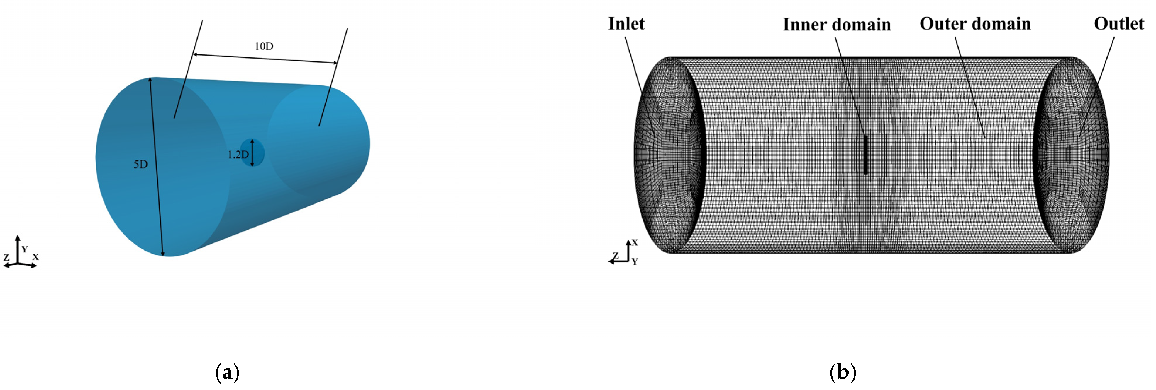
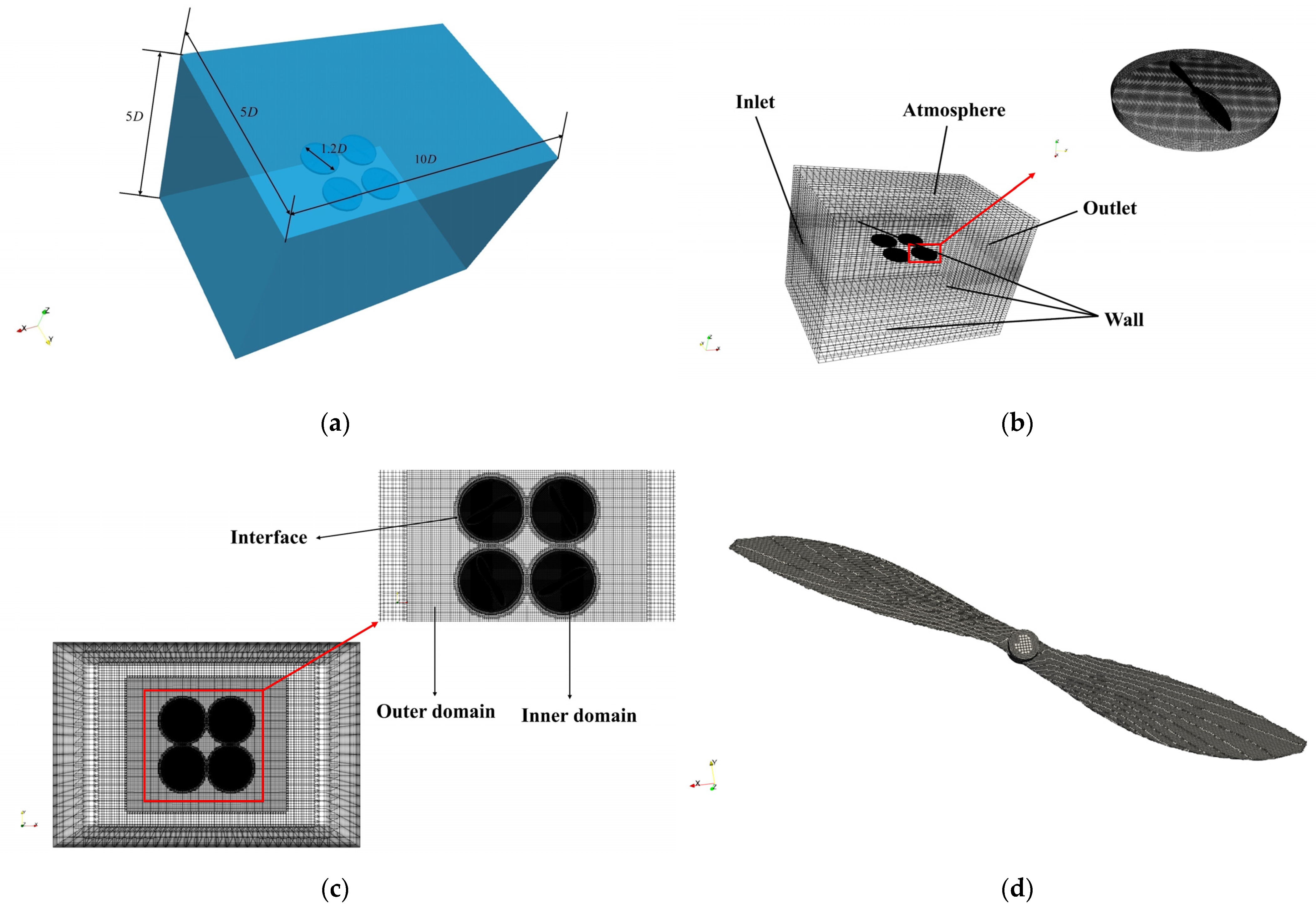
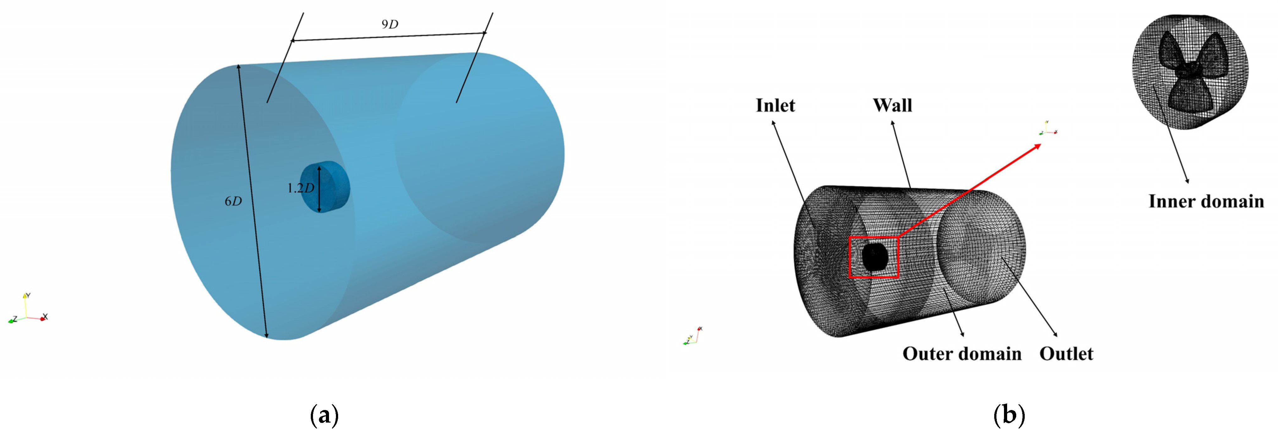
2.1. Modeling of Air Media

The modeling of the air medium of the trans-media aircraft is the same as the modeling of ordinary multi-rotor UAVs, and its motion process includes translation and rotation.

First, the translation of the trans-medium aircraft is discussed. According to Newton’s second law, it can be obtained:

$$\left(\begin{array}{c}0\\ 0\\ T_1+T_2+T_3+T_4\end{array}\right)-\left(\begin{array}{c}0\\ 0\\ Mg\end{array}\right)=M\left(\begin{array}{c}{a}_x\\ a_y\\ a_z\end{array}\right)$$

(1)

In the formula, $T_1$, $T_2$, $T_3$, $T_4$ is the pulling force generated by the air rotor of the aircraft, $M$ is the overall mass of the aircraft across the medium, and $a_x$, $a_y$, $a_z$ is the acceleration of the body in all directions.

Since the pulling force generated by the propeller is expressed in the body coordinate system, there is a transformation relationship between the relative and the whole Earth coordinate system; thus, the result of the above formula in the Earth coordinate system is:

$$R_b^e\left(\begin{array}{c}0\\ 0\\ T_1+T_2+T_3+T_4\end{array}\right)-\left(\begin{array}{c}0\\ 0\\ Mg\end{array}\right)=M\left(\begin{array}{c}{a}_x\\ a_y\\ a_z\end{array}\right)$$

(2)

where $R_b^e$ is the rotation matrix [21] from the body coordinate system to the Earth coordinate system,

$$R_b^n=\left(\begin{array}{ccc}cos\theta cos\psi & cos\psi sin\theta sin\varphi -sin\psi cos\varphi & cos\psi sin\theta +sin\psi sin\varphi \\ cos\theta sin\psi & sin\psi sin\theta +cos\psi cos\varphi & sin\psi sin\theta cos\varphi -cos\psi sin\varphi \\ -sin\theta & sin\varphi cos\theta & cos\varphi cos\theta \end{array}\right)$$

(3)

$\varphi$, $\theta$, $\psi$ represent the roll angle around the x-axis, the pitch angle around the y-axis, and the yaw angle around the z-axis, namely Euler angles.

Substitute (3) into (1) to obtain:

$$\begin{array}{l}\{\begin{array}{c}M\ddot{x}=(cos\varphi sin\theta cos\psi +sin\varphi sin\psi )F\\ M\ddot{y}=(cos\varphi sin\theta sin\psi -sin\varphi cos\psi )F\\ M\ddot{z}=cos\varphi cos\theta *F-Mg\end{array}\\ \end{array}$$

(4)

This results in the equation of the resultant external force and velocity in the dynamic model, that is, the position dynamic model. where $F=T_1+T_2+T_3+T_4$.

Next, the rotation of the trans-medium aircraft is discussed, which is obtained by Euler’s equation [22]:

$$\mathit{J}{\dot{\mathit{\omega }}}^b+{\mathit{\omega }}^b\times \mathit{J}{\mathit{\omega }}^b={\mathit{G}}_a+\mathit{\tau }$$

(5)

In the formula, ${\mathit{\omega }}^b$ represents the angular velocity in the body coordinate system; ${\mathit{G}}_a$ represents the gyro moment; $\mathit{\tau }$ represents the moment generated by the propeller on the body axis, including the rolling moment ${\tau }_x$ around the ${\mathrm{O}}_b{x}_b$-axis, the Pitch moment on the $O_b{y}_b$-axis ${\tau }_y$ and yaw moment around the $O_b{z}_b$-axis ${\tau }_z$.

About the inertia matrix $\mathit{J}$: based on the assumptions made earlier, the inertia matrix can be expressed as:

$$\mathit{J}=\left(\begin{array}{ccc}{J}_{xx}& & \\ & J_{yy}& \\ & & J_{zz}\end{array}\right)$$

(6)

Let ${\mathit{\omega }}_b=\left(\begin{array}{c}{\omega }_x\\ {\omega }_y\\ {\omega }_z\end{array}\right)$, ${\mathit{G}}_a=\left(\begin{array}{c}{G}_{a,\varphi }\\ G_{a,\theta }\\ G_{a,\psi }\end{array}\right)=\left(\begin{array}{c}{J}_{RP}{\omega }_x({\varpi }_1-{\varpi }_2+{\varpi }_3-{\varpi }_4)\\ J_{RP}{\omega }_y(-{\varpi }_1+{\varpi }_2-{\varpi }_3+{\varpi }_4)\\ 0\end{array}\right)$, substitute into (5) formula to obtain:

$$\{\begin{array}{c}{\dot{\omega }}_x=\frac{1}{I_{xx}}\left[{\tau }_x+{\omega }_y{\omega }_z(I_{yy}-I_{zz})-J_{RP}{\omega }_y\Theta \right]\\ {\dot{\omega }}_y=\frac{1}{I_{yy}}\left[{\tau }_y+{\omega }_x{\omega }_z(I_{zz}-I_{xx})+J_{RP}{\omega }_x\Theta \right]\\ {\dot{\omega }}_z=\frac{1}{I_{zz}}\left[{\tau }_z+{\omega }_x{\omega }_y((I_{xx}-I_{yy}))\right]\end{array}$$

(7)

where $\Theta =-{\varpi }_1+{\varpi }_2-{\varpi }_3+{\varpi }_4$.${\varpi }_1$,${\varpi }_2$,${\varpi }_3$,${\varpi }_4$ is the rotational speed of the motor that drives the air rotor.

The above is the dynamic modeling of the trans-medium aircraft (air medium), which represents the relationship between the input resultant external force, the resultant external torque, and the output velocity and angular velocity.

Next, kinematic modeling of aircraft across media needs to be discussed (air medium), which describes the quantitative relationship between the velocity and angular velocity of the input and the position and attitude of the output.

The equation for the position is simple and can be expressed as:

$${\dot{\mathit{P}}}^e={\mathit{v}}^e$$

(8)

In the above formula, ${\mathit{P}}^e={\left(\begin{array}{ccc}x& y& z\end{array}\right)}^T$ is used to represent the coordinate position of the aircraft in the Earth coordinate system, and then, Formula (8) is expanded to obtain:

$${\left(\begin{array}{ccc}\dot{x}& \dot{y}& \dot{z}\end{array}\right)}^T={\left(\begin{array}{ccc}{v}_x& v_y& v_z\end{array}\right)}^T$$

(9)

Next comes the equation for attitude.

The rate of change of the attitude angle is related to the rotational angular velocity of the body as follows:

$$\dot{\mathit{\Omega }}=\mathit{\Gamma }•{\mathit{\omega }}^b$$

(10)

In the formula, $\mathit{\Omega }$ is the three attitude angle (Eulerian angle) matrix of the trans-medium aircraft, $\mathit{\Gamma }$ is the attitude calculation coordinate transformation matrix, which measures the transformation relationship between the rate of change of the attitude angle and the rotational angular velocity of the body. Thus, the above formula can be fully expanded:

$$\left(\begin{array}{c}\dot{\varphi }\\ \dot{\theta }\\ \dot{\psi }\end{array}\right)=\left(\begin{array}{ccc}1& tan\theta sin\varphi & tan\theta cos\varphi \\ 0& cos\varphi & -sin\varphi \\ 0& sin\varphi /cos\theta & cos\varphi /cos\theta \end{array}\right)\left(\begin{array}{c}{\omega }_x\\ {\omega }_y\\ {\omega }_z\end{array}\right)$$

(11)

In the case of small disturbance, that is, under the premise that the change of each angle is small, the $\mathit{\Gamma }$ matrix is a unit matrix; thus, it can be obtained:

$$\left(\begin{array}{c}\dot{\varphi }\\ \dot{\theta }\\ \dot{\psi }\end{array}\right)=\left(\begin{array}{c}{\omega }_x\\ {\omega }_y\\ {\omega }_z\end{array}\right)$$

(12)

Thus far, the model establishment for the trans-medium aircraft (air medium) has been completed.

Remark 1.

The reason for the left-multiplied rotation matrix in Equation (2) is that the body coordinate system performs a rotation about the geostationary coordinate system. Equation (3), as a rotation matrix, reflects the equivalent relationship of the transformation from the Earth coordinate system to the airframe coordinate system.

Remark 2.

Equation (5) describes the differential equation for the motion of a rigid body, in the motion of a rigid body around a fixed point, reflecting the relationship between angular velocity, angular acceleration and the moment on the rigid body.

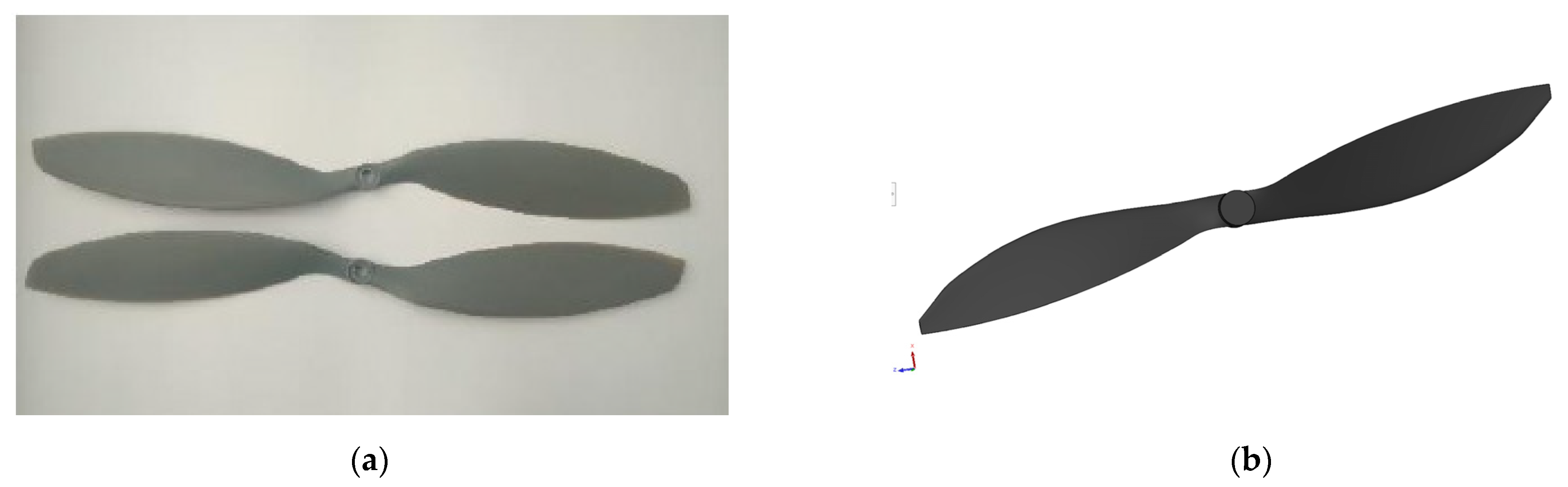
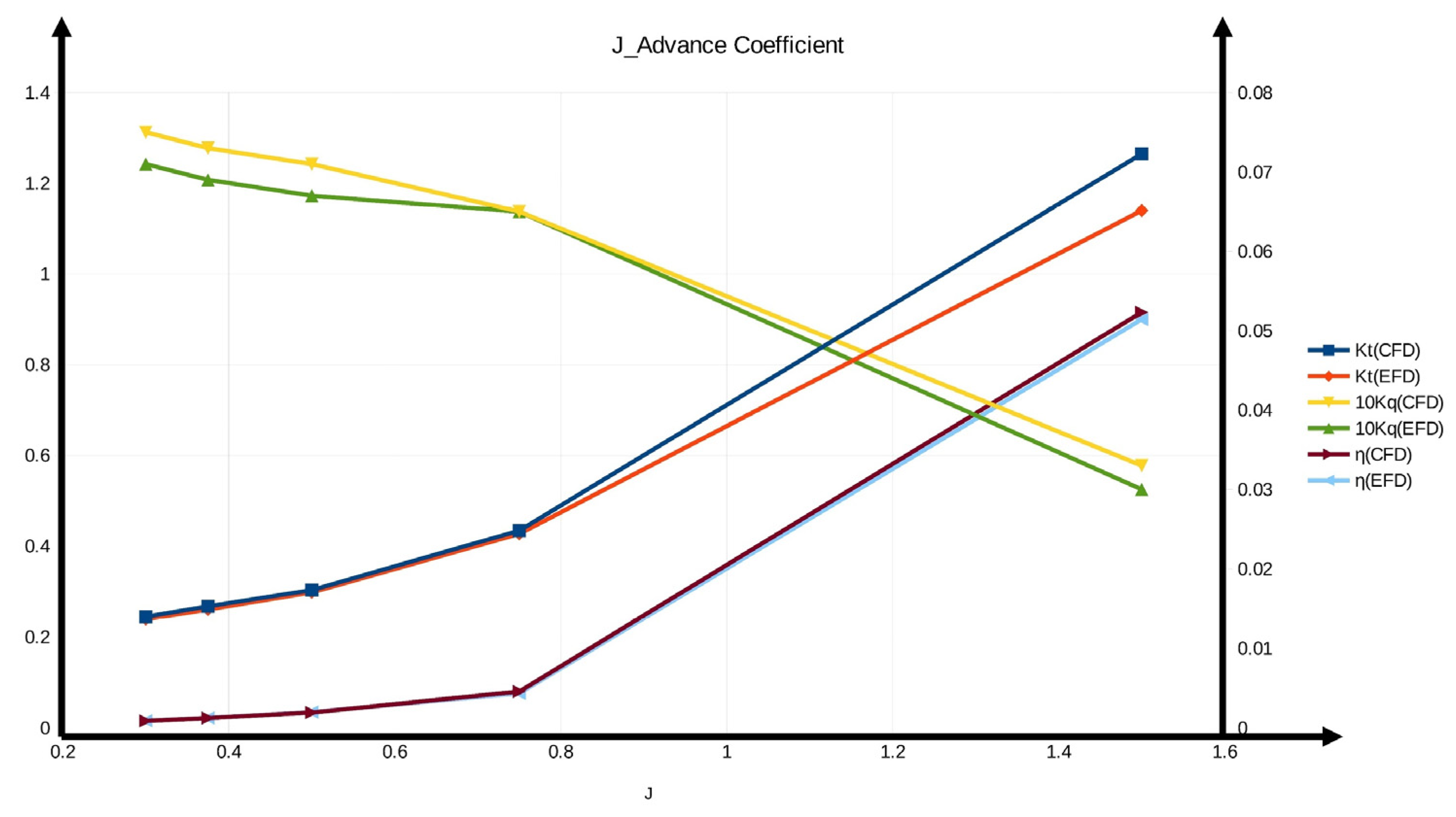
2.2. Establishment of Underwater Propeller Propulsion Model

First, underwater dynamics modeling needs to be considered. When a trans-medium aircraft moves underwater, it will drive a small part of the fluid around the aircraft to move at the same time, and this small part of the fluid acts on the aircraft; thus, the additional mass of the aircraft during motion needs to be considered [23]. The physical expression of this additional mass is that the inertial coefficient of the aircraft produces an increment ${\lambda }_{ik}$ ($i,k=1,2,\cdots 6$, representing six directions). The motion of this small part of the fluid can be regarded as a rigid-body-like motion, that is, the motion of the fluid is a rigid-body-like motion at the same speed as the trans-medium aircraft. There is only one symmetry plane $O_b{y}_b{z}_b$ for the trans-medium aircraft; thus, there are 12 inertial coefficient increments ${\lambda }_{ik}$ that are not zero. Therefore, the underwater dynamic model of the trans-medium aircraft defined by generalized parameters is as follows:

$$\mathit{M}\dot{\mathit{v}}+\mathit{W}(v)\mathit{v}={\displaystyle \sum \mathit{F}}$$

(13)

In the formula, $\mathit{M}$ is the generalized mass matrix of the trans-medium aircraft, $\mathit{W}(v)$ is the external force coefficient matrix received, and ${\displaystyle \sum \mathit{F}}$ is the external force received by the fluid resistance, lift, etc., which can be solved by the OpenFOAM open source numerical platform.

Next, model the underwater kinematics of the trans-medium aircraft. The purpose of kinematic modeling is to convert the coordinate variables in the body coordinate system to the Earth coordinate system through the coordinate transformation matrix. The modeling idea is consistent with the previous air medium.

$$\left(\begin{array}{c}\dot{p}\\ \dot{\varsigma }\end{array}\right)=\left(\begin{array}{cc}{({\mathit{R}}_e^b)}^{-1}& {\mathit{0}}_{3\times 3}\\ {\mathit{0}}_{3\times 3}& {\mathit{T}}_{\varsigma }(\varsigma )\end{array}\right)•\left(\begin{array}{c}\mathit{v}\\ \mathit{\omega }\end{array}\right)$$

(14)

Then, the kinematic equation can be expressed in the form of generalized velocity and generalized position:

$$\dot{\mathit{P}}=\mathit{J}(R)\mathit{V}$$

(15)

$$\mathit{J}(R)=\left(\begin{array}{cc}{({\mathit{R}}_e^b)}^{-1}& {\mathit{0}}_{3\times 3}\\ {\mathit{0}}_{3\times 3}& {\mathit{T}}_{\varsigma }(\varsigma )\end{array}\right)$$

(16)

$${\mathit{R}}_e^b=\left(\begin{array}{ccc}cos\theta cos\psi & cos\theta sin\psi & -sin\theta \\ sin\varphi sin\theta cos\psi -cos\varphi sin\psi & cos\varphi cos\psi +sin\varphi sin\theta sin\psi & sin\varphi cos\theta \\ sin\varphi sin\psi +cos\varphi cos\psi sin\theta & cos\varphi sin\theta sin\psi -sin\varphi cos\psi & cos\varphi cos\theta \end{array}\right)$$

(17)

In the formula, $\mathit{P}$ is the generalized position matrix, $\mathit{V}$ is the generalized velocity matrix, ${\mathit{T}}_{\varsigma }(\varsigma )=\mathit{\Gamma }$ (11), $\varphi$, $\theta$, $\psi$ are the roll angle, pitch angle, yaw angle of the aircraft as mentioned above.

Remark 3.

The main diagonal element ${\mathit{R}}_e^b$of the matrix in Equation (16) corresponds to the coordinate transformation matrix of the velocity, and the element ${\mathit{T}}_{\varsigma }(\varsigma )$corresponds to the transformation matrix of the angular velocity and the rate of change of the Euler angles.

2.3. Multimedia Spanning Model Establishment

When the aircraft is performing multi-medium spanning, the body is subject to the combined action of the air medium and the water medium. Therefore, in the vertical plane, the relationship between the buoyancy of the body and the propeller tension and gravity needs to be considered. In the horizontal plane, there are two cases: (1) the aircraft across the medium is in still water conditions, and no force is considered in the horizontal plane; (2) under non-stationary conditions, the flow resistance of the aircraft during the medium crossing process needs to be considered.

In the vertical plane, when the body crosses the medium vertically, the force diagram of the trans-medium aircraft is as follows, as shown in Figure 3.

For the free entry stage, there are:

$$F_b=\rho g{S}_{section}H$$

(18)

$$G-F_b=M\ddot{z}$$

(19)

$H$ is the immersion depth of the aircraft, $z$ is the displacement of the aircraft in the vertical direction.

When the aircraft is out of water (uniform speed), there are:

$$F_T+F_b=G$$

(20)

$$F_T=T_1+T_2+T_3+T_4$$

(21)

$$T_i=C_T\rho n_i{}^2{D}^4, i=1 ,2 ,3 , 4$$

(22)

In the above formula, $T_i$ is the thrust generated by the propeller, $C_T$ is the rotational speed of the propeller, $D$ is the diameter of the propeller, and $n_i$ is the rotational speed of the propeller.

When the trans-medium aircraft enters and leaves the water at a certain attitude angle, and the aircraft does not completely leave the water surface, as long as the attitude changes, the size of the buoyancy and the position of the center of buoyancy will change, and the aircraft needs to generate a restoring torque to overcome this attitude change [24]. The magnitude of the restoring moment is related to gravity and buoyancy.

Since the pitch and roll attitude changes of the trans-medium aircraft in this paper have the same effect on the force during the multi-medium crossing process of the aircraft, the two are analyzed together, and a generalized attitude angle $\gamma$ is defined. Figure 4 is a schematic diagram of the force when the trans-medium aircraft enters the water at a certain attitude angle.

Define the length of one side of the aircraft submerged in the water as $L$, the displacement of the center of gravity in the vertical direction as $z$, and the radial distance between the motor and the center of gravity of the aircraft as $r$, and the center of the restoring moment as the center of the cross-section between the aircraft and the water surface, then there are:

$$M_R=-F_b•\frac{L}{2}-\frac{Gzcos\gamma }{sin\gamma }$$

(23)

where $F_b$ has been obtained from (16). When the aircraft enters the water in the pitch attitude, $\gamma =\theta$; when the aircraft enters the water in the roll attitude, $\gamma =f$.

In the horizontal plane, it is considered that the water surface of the trans-medium aircraft is in a non-stationary state, and there is an impact effect of waves on the body. Therefore, in the water entry and exit stage, the trans-medium aircraft has a certain displacement in the horizontal plane, and its displacement expression is expressed by Newton’s second law, which can be obtained:

$$S_v{\mathit{p}}_w=\mathit{M}\ddot{\mathit{x}}$$

(24)

In the formula, ${\mathit{p}}_w$ is the wave force action matrix, $S_v$ is the cross-sectional area of the wave action body, and $x$ is the displacement matrix of the trans-medium aircraft.

At this point, the dynamic and kinematic model of the trans-medium aircraft has been established. The following, Figure 5 and Figure 6, are schematic diagrams of the complete multi-medium crossing process of the trans-medium aircraft.

3. Numerical Simulation Based on OpenFOAM Open-Source Platform

Through the selection and layout design of each component of the trans-media aircraft, a parametric mechanical structure model of the trans-media aircraft is established. Import the parametric model of the aircraft into the OpenFOAM platform tool for simulation analysis.

Consistent with the previous analysis idea, the motion process of the trans-medium aircraft is analyzed in sections. The specific processes simulated in this paper are: (1) aerodynamic simulation analysis of a single air medium; (2) hydrodynamic simulation analysis of a single underwater medium; (3) simulation analysis of the aircraft entering the water vertically and at a certain attitude angle; (4) simulation analysis of the aircraft leaving the water surface vertically.

3.1. Fluid Governing Equations

The solution to the medium flow problem is the solution to the Navier–Stokes equation, which is the theoretical basis for describing the medium flow. The flight speed of the trans-medium aircraft model established in this paper is lower than the speed of sound; thus, the medium in which it is located can be regarded as an incompressible flow. Incompressible flow governing equations include continuity equation and momentum equation, as follows [25]:

$$\{\begin{array}{c}\nabla •\mathit{U}=0\\ \frac{\partial \mathit{U}}{\partial t}+\nabla •(\mathit{U}{\mathit{U}}^T)=-\frac{1}{\rho }\nabla p+\nabla •(\upsilon \nabla \mathit{U})+\mathit{S}\end{array}$$

(25)

where $U$ is the fluid velocity vector, $p$ is the fluid pressure, and $\upsilon$ is the fluid kinematic viscosity.

The essential work of numerical simulation for fluid media is to solve the above equations, but for the above equations, it is difficult to obtain their analytical solutions in the sense of actual equations; thus, it is necessary to numerically discretize their differential equations and obtain matrix equations through discretization processing. The solution of the equation is the numerical solution of the equation. Although the numerical solution is not the real solution of the original equation, the error with the real solution can be reduced by selecting a suitable discretization method and matrix solving algorithm to approach the real solution.

Remark 4.

Equation (25) is a simplification of the N-S equation, which exhibits the continuity equation and the momentum conservation equation for incompressible flow. In this study, under low velocity conditions, the medium can be regarded as a continuous incompressible form.

3.2. Turbulence Model

During the movement of the trans-medium aircraft, the flow of the fluid medium in which it is located is irregular, multi-scale, and structured, that is, three-dimensional unsteady flow, which has strong numerical diffusivity and numerical dissipation [26]. No matter how complex the turbulent motion is, the unsteady continuity equations and Navier–Stokes equations are still applicable to the instantaneous motion of turbulent flow. However, the strong transient nature and nonlinearity of turbulent flow make it impossible to accurately describe all the details related to the three-dimensional time of turbulent flow by analytical methods. Changes in the mean flow field are often caused by turbulence. In this way, mathematical calculation methods for different simplifications of turbulent flow have emerged. It reduces the computational cost, and by simplifying the operation, practically valuable physical phenomena can be effectively extracted. The turbulence model implanted in this paper based on the OpenFOAM (OpenFOAM V-2112) open source platform is the kOmegaSST model, which is a hybrid model of the kEpsilon model and the kOmega model. The purpose of the mixture is to use the kOmega model with a better effect on the reverse pressure gradient near the wall and use the kEpsilon model that is insensitive to incoming flow parameters elsewhere [27]. Its model equation is as follows:

Turbulence intensity $k$ equation:

$$\frac{\partial \rho k}{\partial t}+\nabla (\rho kU)=\nabla \left[(\mu +\frac{{\mu }_z}{{\sigma }_k})\nabla k\right]+p_k-b_k\rho k\omega$$

(26)

Turbulence frequency $\omega$ equation:

$$\frac{\partial \rho \omega }{\partial t}+\nabla (\rho \omega U)=\nabla \left[(\mu +\frac{{\mu }_z}{{\sigma }_{\omega }})\right]+a\frac{\omega }{k}{p}_k-b_{\omega }\rho k{\omega }^2$$

(27)

In the above formula, $p_k$ is the turbulent kinetic energy generated by the laminar velocity gradient, ${\sigma }_k$ and ${\sigma }_{\omega }$ are the Prandtl number of the turbulent energy; the eddy viscosity is ${\mu }_{}=-\rho k/\omega$.

Remark 5.

Equation (26) and Equation (27) are simplified calculations for solving the turbulent flow of the N-S equation. Due to the strong transient nature of the turbulent flow, Reynolds averaging is performed on the physical quantities of the flow field in the time domain. After averaging, the N-S equation is not closed; thus, two variable equations a and b are introduced for solving. The two variable equations are semi-empirical formulas, which are summed up from experimental phenomena.

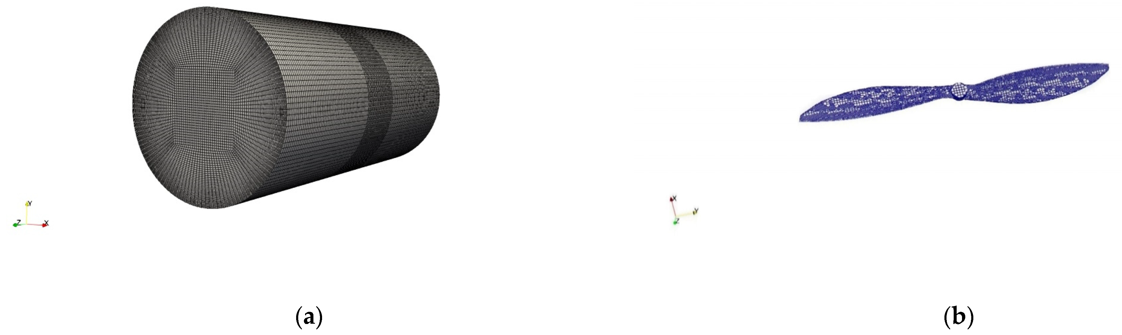
3.3. Simulation Analysis of Multi-Medium Crossing for a Trans-Medium Aircraft

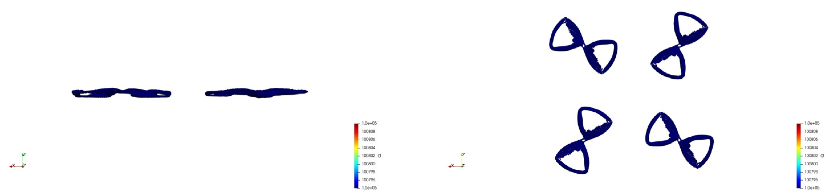
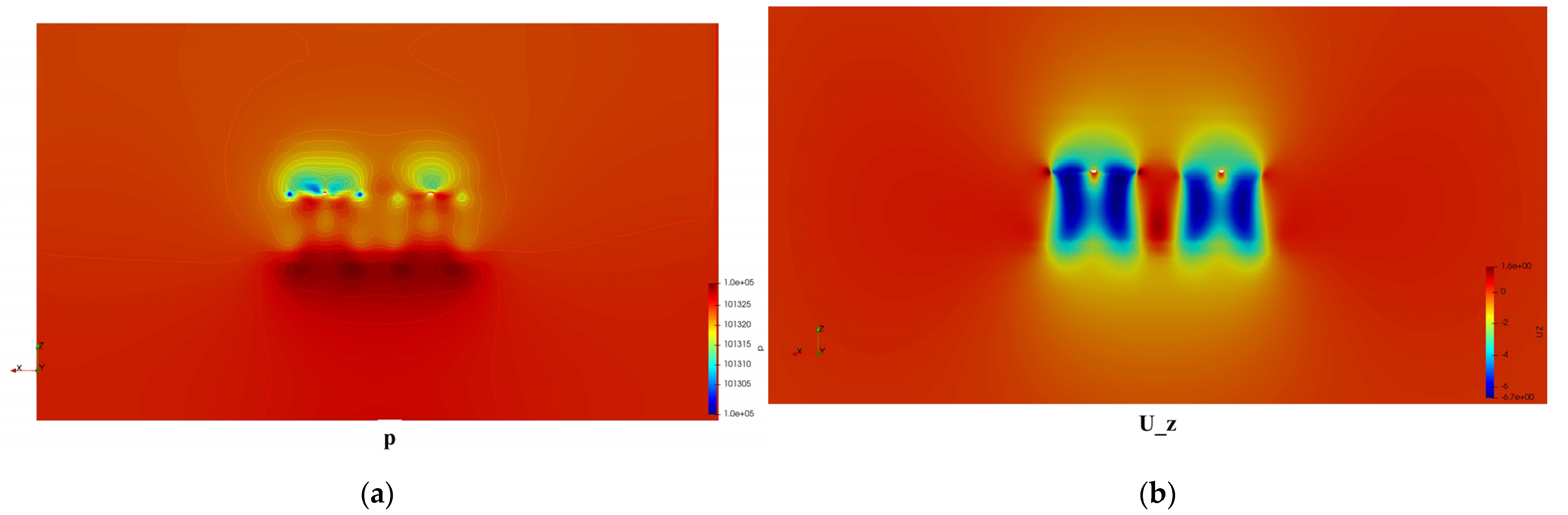
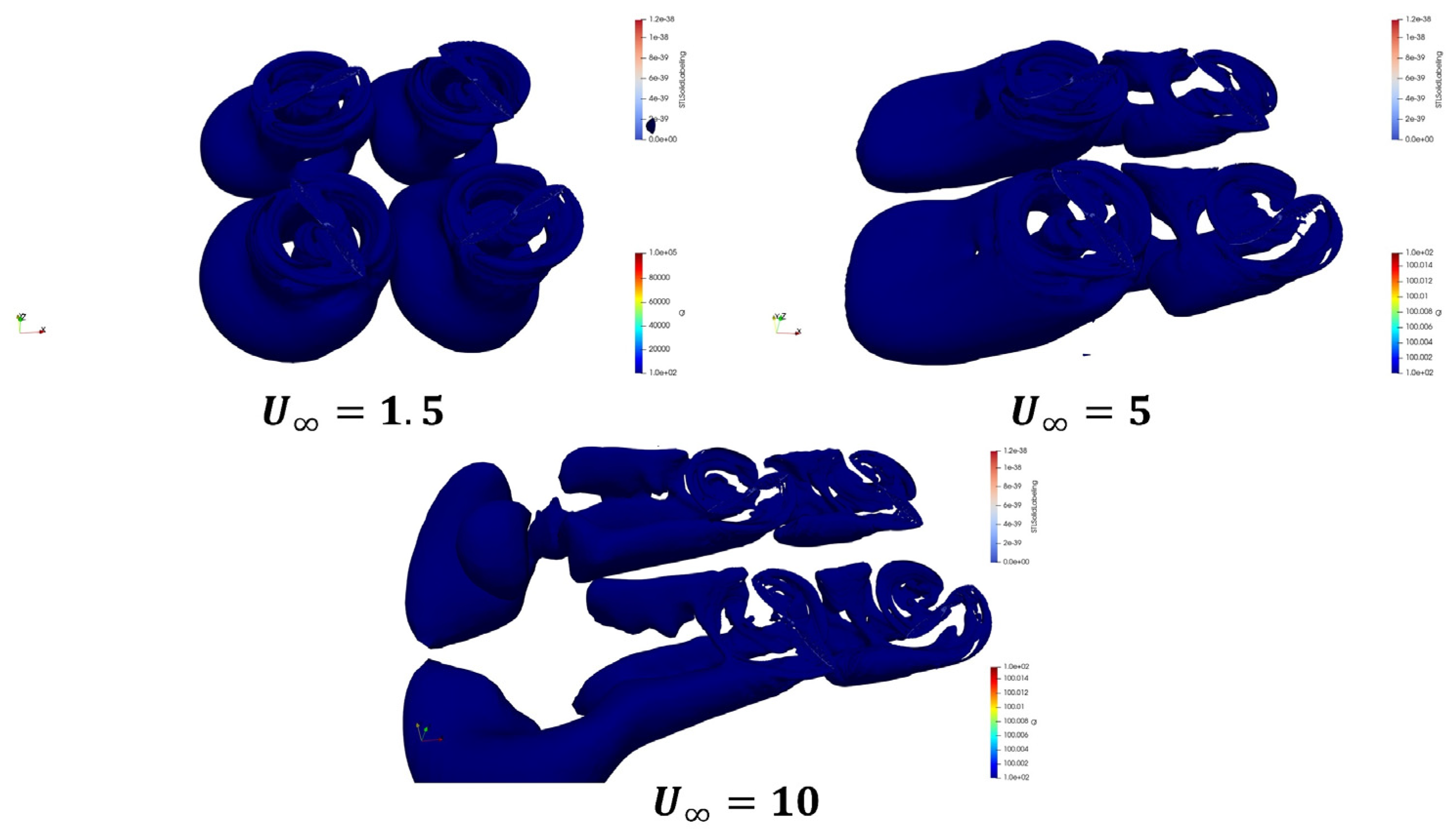
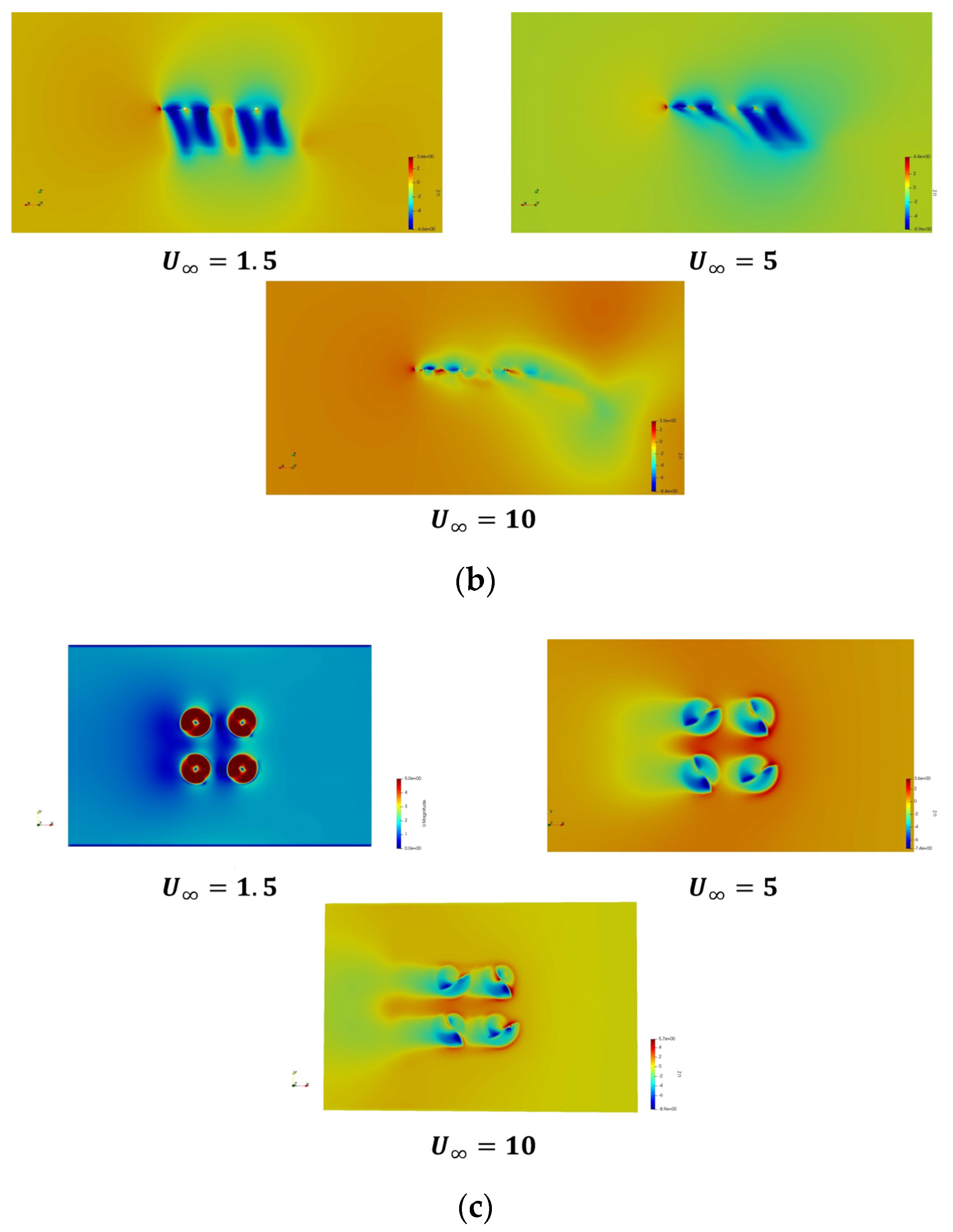
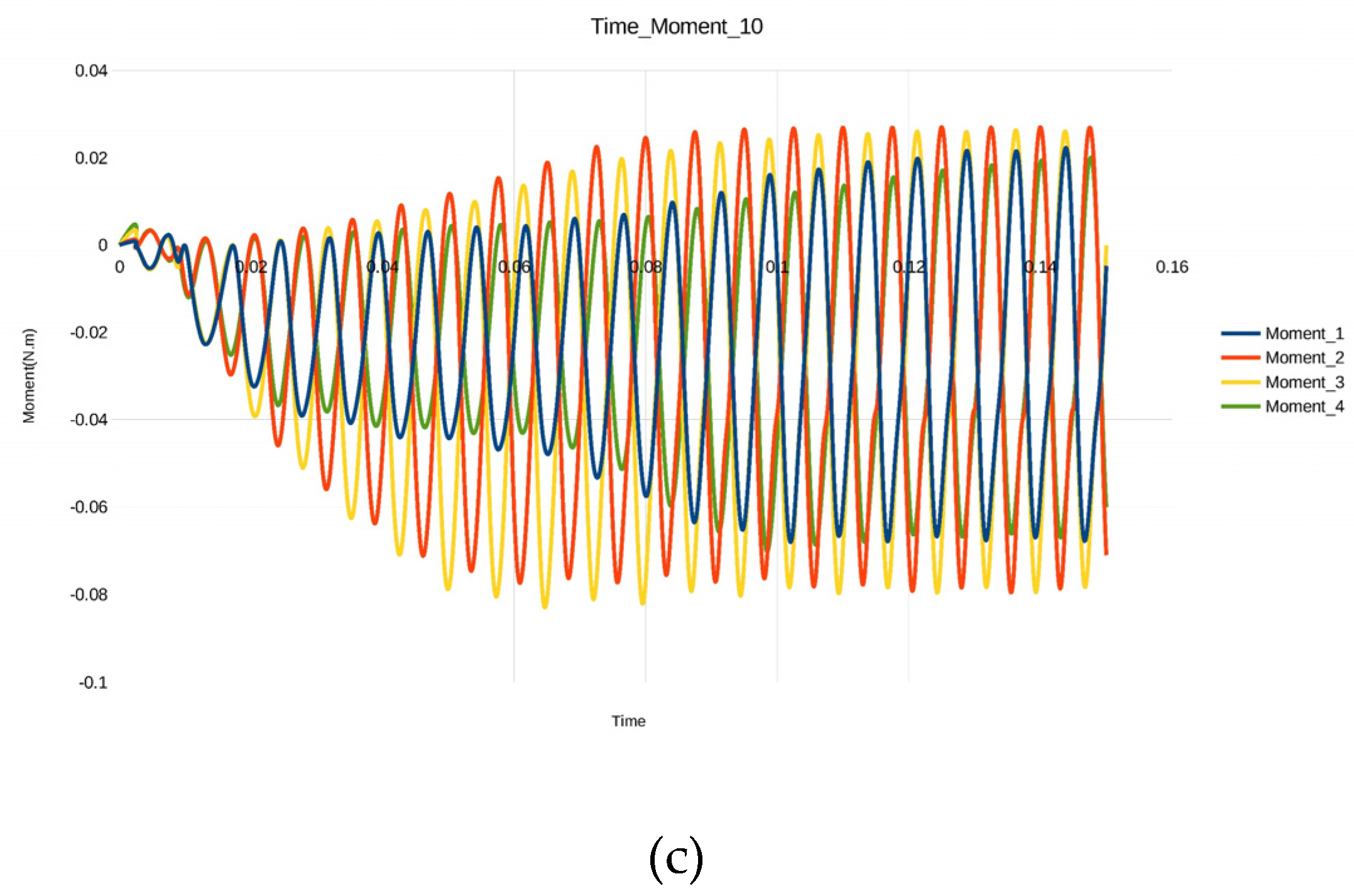
3.3.1. Air Single Medium Aerodynamic Analysis

The carrier of the air single-medium analysis is the air rotor; thus, first, a basic mechanical characteristic analysis of the air rotor of the trans-medium aircraft designed in this paper is carried out. The air rotor parameters for this article are as follows: Model APC1047SF, which has a diameter of 10 inches and a pitch of 4.7 inches. The physical and model diagrams are as follows, as shown in Figure 7.

Next, the rotor flow field is discretized, and the computational domain of the flow field is divided into two parts: the outer domain and the inner domain, as shown in Figure 8. The inner domain is centered on the rotating shaft of the air rotor, with a diameter of 1.2D (D is the rotation diameter of the blade); the outer domain is the outer cylindrical area of the rotor, with a length of 10D and a diameter of 5D.

In the fluid computing domain, the interface between the inner domain and the outer domain adopts a slip mesh; the purpose is to not only realize the high-speed rotation of the air rotor around the axis at a certain speed but also to save computing resources. This movement process is as described above in that its medium flow is an unsteady flow. The computational domain has meshed with the “blockMesh” mesh algorithm and “SnappyHexMesh” mesh algorithm implanted in the OpenFOAM open source platform.

The meshing method is based on OpenFOAM this time: the O-type mesh topology method is used to define the “blockMesh” parameter dictionary for background meshing, and then, the “snappyHexMesh” tool is used to mesh the air rotor and establish the interface between the inner domain and the outer domain. Mesh division is shown in Figure 9.

The completion of the grid division means that the pre-processing part of the simulation process has been completed. Next, the above-mentioned physical process is numerically solved through the matrix solving algorithm implanted in the OpenFOAM platform, and the required results are processed and analyzed. The kOmegaSST turbulence model is used, and the boundary conditions are set as follows: the inlet boundary of the outer domain of the cylinder adopts the velocity inlet condition, the outlet boundary adopts the pressure outlet condition, and the cylindrical boundary of the cylinder adopts the wall surface condition.

Through the variable parameter analysis of different rotational speeds of the air rotor, the mechanical characteristics and flow field characteristics under different rotational speeds are compared. In this study, the rotational speeds of the air propellers were set to 2000, 3000, 5000, 7000, and 8000 (unit $round\times mi{n}^{-1}$), respectively. Figure 10 shows the comparison between the thrust of the air rotor obtained by numerical simulation at different speeds and the experimental thrust of the APC1047SF blade.

It can be seen from the above figure that the overall calculation error is not large, and the error between the simulated value and the experimental value can be ignored under the condition of low speed. As the rotational speed increases gradually, at higher rotational speeds, the error between the simulated value and the experimental value also increases gradually, but is within a reasonable error range. The reason why this error gradually increases at higher rotational speeds is that there is an error in the meshing accuracy under high rotational speed conditions, and high-resolution meshes are not used for high rotational speed conditions. However, because of saving computing power, this study uses a medium-resolution grid within the range of ensuring a reasonable error.

Figure 11 shows the pressure cloud map and speed cloud map of a certain section of the air rotor under different rotational speed conditions.

It can be seen from the change in the above pressure cloud diagram that the air rotor rotates at a certain speed, and the tip of the blade generates a low-pressure area due to high-speed friction with the air. The entire blade produces a symmetrically distributed pressure vortex ring backward along the direction of the central axis of rotation. This is because, in the case of airflow disturbance, there is a pressure difference between the front and rear positions of the vortex ring, which leads to the generation of the phenomenon of surrounding flow, thereby generating a pressure vortex. The creation of pressure vortices is also what causes the thrust of the air rotor to drop. It can be seen from the figure that there is a pressure difference in the flow field before and after the rotor, and the rotor generates thrust due to the effect of this pressure difference.

It can be seen from the above velocity cloud diagram that the airflow at the rear end of the blade produces a symmetrically distributed high-speed band due to the high-speed rotation of the rotor, and it can be found that the paddle where the blade is located has a current-collecting effect, and the airflow passes through this paddle. The airflow flows in from the front end of the paddle disc, and after the constriction of the current collecting effect of the paddle disc, the airflow flowing to the rear end rotates and takes on a spiral shape, which generates the circumferential induced velocity.

Figure 12 shows a schematic diagram of the change of the tip vortex under each speed condition:

As the rotational speed continues to increase, the more severe the disturbance of the blade tip is, the more obvious the dragging effect of the blade tip wake is in the figure.

In order to accurately capture the vortex structure in the flow field, the Q criterion [28] is applied to the post-processing vortex capture technology. Figure 13 shows the schematic diagram of the vortex structure in the flow field under various rotational speed conditions ($Q\in \left[-100,100\right]$).

It can be seen from the above figure that the wake vortex of the rotor is symmetrically distributed at different rotational speeds. As the rotational speed increases, the structure of the wake vortex becomes more complex. The more severe the airflow disturbance is, the more serious the gas disturbance is.

Next, take the rotational speed RPM = 7000 $round\times mi{n}^{-1}$ as an example, and focus on analyzing the specific numerical change relationship of each physical quantity in the flow field.

To find the variation relationship of each physical quantity with time and space, the following Figure 14 shows the variation relationship between the position and physical quantity along the rotation axis from left to right and the variation relationship between the time step and physical quantity solved under different position conditions (top and bottom of paddle).

It can be seen from Figure 14a that between 1 and 1.5 m on the abscissa (the area near the paddle disc) the pressure will show a high- and low-pressure area, the pressure at the lower part of the paddle disc will increase, and a high-pressure area will appear, while the upper-pressure will drop, and a low-pressure area will appear, and with the advancement of the time step, the amplitude of the upper-pressure drop will increase, resulting in an increase in the upper and lower-pressure difference, which is the reason for the increase in the thrust of the blade at the beginning. Figure 14b shows that there is a pressure difference between the upper and lower surfaces of the propeller disc, which is the reason for the thrust generated by the previously mentioned propeller blades. Figure 14c reflects that the fluid velocity peaks in the area near the paddle disk, and the position of the peak gradually moves down with the increase in the time step, which is consistent with the results presented in the previous velocity cloud map. Figure 14d reflects the process of increasing the velocity of the upper and lower surfaces of the paddle disc in the initial time. With the increase in time, the velocity gradually tends to be stable, and the velocity on the lower surface is always greater than that on the upper surface.

The above is the analysis of the aerodynamic characteristics of the air blades of the trans-medium aircraft. Next, it is necessary to carry out a numerical simulation study on the air flight characteristics of the trans-medium aircraft, and the method used is the same as the previous one. The mesh division is shown in Figure 15:

Next, the numerical simulation method is used to simulate the hovering and forward flight motion of the trans-medium aircraft, and the obtained simulation results are physically analyzed.

Figure 16 shows the structure of the rotor tip vortex in the hovering state of the whole machine. It can be seen from the figure that the wake vortex generated by the friction between the blade and the air will continuously impact the arm of the machine, thereby causing the body to vibrate.

Figure 17 shows the numerical simulation cloud image of the hover state. It can be seen from the pressure and velocity contour that a high-pressure area is generated at the lower part of the paddle plane, and due to the large velocity interference at the lower part, the flow phenomenon is caused, resulting in a pressure vortex, which is also the reason for the drop in lift. A low-pressure area is generated in the upper part such that the pressure difference between the upper and lower surfaces is generated, which is the key factor for the rotor to generate lift [29].

To study the aerodynamic interference of the trans-medium aircraft in the forward flight state, this paper sets the forward flight inclination angle of the trans-medium aircraft as 10°, the blade speed as 4000 $round\times mi{n}^{-1}$, and the forward flight speed as 1.5 $m•s^{-1}$, 5 $m•s^{-1}$. There are three cases of 10 $m•s^{-1}$, and the forward ratio of the aircraft is 0.289.

Figure 18 is a comparison of the rotor wake structures at three forward flight speeds. It can be seen from the figure that the wake is dragged out from the blades and the fuselage, and the flow to the downstream area induces the entire flow field, and with the increase in the forward speed, the inclination of the trailed wake is also larger, and the flow field fluctuation is also more complicated.

Figure 19 shows the contour of the flow field pressure and velocity change of the trans-medium aircraft under different forward flight speeds. Different from the hovering state, in the forward flight state of the trans-medium aircraft, the wake will move backward, and it is behind the flight. Compared with the hovering state, the impact of the propeller on the aerodynamic force of the fuselage is greatly reduced, and the wake of the propeller in the front will hit the fuselage, which is the main reason for the change in the aerodynamic force of the fuselage.

Through the analysis of the above longitudinal pressure and velocity contour, it can be seen that with the increase in the forward flight speed, the pressure vortex gradually shifts to the rear, and the direction of the high-speed airflow region at the rear is the same as that of the pressure vortex. Through the analysis of the axial velocity cloud diagram of the propeller disc, it can be seen that the axial velocity of the four blades is all downward, and the wake of the flow around the cloud diagram gradually moves backward with the increase in the forward speed. It can be seen from the wake structure diagram in Figure 19 that the blade is impacted by the wake of the front blade, and the aerodynamic characteristics of the rear blade are most disturbed during the flight.

Figure 20 is a graph showing the variation of the force characteristics of each blade with time. It can be seen from the figure that with the forward flight process of the aircraft, the force characteristics of each blade change periodically, and due to the backward movement of the forward flight trail, the forward flight effect of each blade is also different. It can be seen from the graph that the fluctuation of the force characteristics of the No. 2 and No. 3 blades is significantly higher than that of the No. 1 and No. 4 blades. This is because the wake has a greater effect on the No. 2 and No. 3 blades than on the No. 1 and No. 4 blades. The unbalanced fluctuation of the force characteristics causes the body to generate an unbalanced moment during forward flight [30].

3.3.2. Hydrodynamic Analysis of Single Underwater Medium

The carrier that provides underwater power for the trans-medium aircraft is the underwater propeller, and the hydrodynamic performance of the underwater propeller plays a vital role in the underwater propulsion of the trans-medium aircraft. At present, open water tests are usually used to determine the hydrodynamic performance of propellers [31]. With the rapid development of computer-aided software and the in-depth study of the mathematical model of fluid dynamics, a numerical simulation based on the CFD method is widely used in propeller performance optimization and dynamic characteristic analysis.

In this paper, two pairs of 60 mm propellers are used, and the underwater thrust system is arranged in a “cross” shape at the duct of the aircraft. First, it is necessary to numerically analyze the water performance of a single propeller. By implanting a numerical algorithm based on the OpenFOAM open source platform, its single propeller is divided into the flow field area, and the division form and solution algorithm are consistent with the method used for the analysis of the aerodynamic characteristics of the air rotor. Figure 21 is a schematic diagram of the grid area division for the numerical analysis of the propeller’s water performance.

To quantitatively describe the hydrodynamic performance of the underwater propeller [32], the numerical simulation method is used to accurately evaluate the propeller’s water performance parameters. The specific embodiment is to obtain the change curve diagram of its thrust coefficient $K_T$, torque coefficient $K_Q$ and efficiency ${\eta }_0$ by changing the propeller advance coefficient, as shown in Figure 22.

It can be seen from the above figure that there is a certain calculation error between the CFD numerical simulation results and the experimental propeller hydrodynamic performance curve results. For $K_T$ and ${\eta }_0$, under the condition of a low advance coefficient, the error can be ignored. The calculation error also increases, and the overall parameter error is within the allowable range of 5%, which meets the actual engineering requirements.

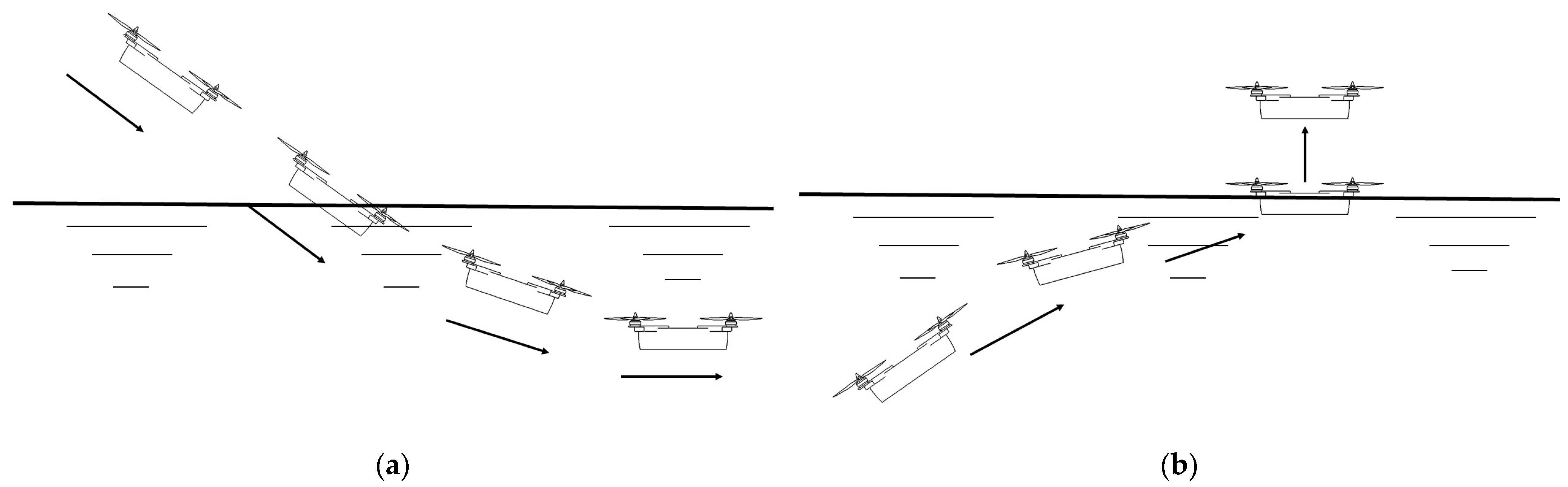
3.3.3. Numerical Simulation of Water Entry and Exit for a Trans-Medium Aircraft

The problem of entering and leaving water across the medium involves the dynamic grid problem. During the solution process, the motion deformation of the grid will have a huge impact on the solution accuracy and the convergence of the solution. The overset grid method [33] is used in the numerical simulation of water entry and exit of a trans-medium aircraft [34]. The overset grid method needs to establish two sets of grids. The flow field where the external trans-media aircraft is located is used as the background grid, and the trans-media aircraft itself is used as the overset grid. The overset grid moves in the background grid. Interpolation is used for the numerical transfer, which does not involve grid deformation; thus, the stability of the solution is guaranteed. However, the two sets of grids need to interpolate each other during the solution process; thus, its calculation time is longer than that of traditional dynamic grids. The water entry and exit process of a trans-medium aircraft is a mirror image process; thus, this paper conducts a numerical simulation of its water entry process. Figure 23 is a schematic diagram of the meshing of the water entry process of the trans-medium aircraft.

In this paper, the initial conditions for the entry of the trans-medium aircraft into the water are set as follows: the entry height is 0.4 m, the initial velocity of entry into the water is 0, and the free-falling body hits the water surface and enters the water body under the action of gravity. In order to verify the performance of the trans-medium aircraft entering the water at different angles, this paper sets its water entry angles as 0°, 10°, 20°, 30°, and 40°. The pressure and speed of the body movement with the time curve are shown in Figure 24.

It can be known from the pressure curve that the load pressure peak of the body is different when entering the water at different angles, and the peak size gradually decreases with the increase in the angle. This reflects that the impact on the vertical entry and exit of the cross-medium aircraft is significantly greater than the impact on the oblique entry and exit of the water. In general, in the water entry stage of the trans-medium aircraft, the load pressure of the body reaches the maximum at the moment of contact with the water surface, and after the water entry process is completed, the load gradually tends to be stable. It can be known from the speed curve that as the water entry angle increases, the speed of the body changes more gently, which corresponds to the previous pressure curve results. The two together indicate that it is most reasonable for the body to enter the water within a limited range of inclination angles.

It can be seen from Figure 25 that when entering the water vertically, the yaw attitude of the cross-medium aircraft changes. When the inclination angle enters the water, the pitch attitude changes more violently, and with the increase in the water entry angle, the angular velocity of the attitude change is larger.

The schematic diagram of the specific physical process of a trans-medium aircraft entering water is shown in Figure 26.

It can be seen from the above figure that the trans-medium aircraft roughly includes three stages in the process of entering the water: the impact of the contact moment, the open cavitation with large deformation of the free surface, and the water movement after the open cavitation is closed. When a trans-medium aircraft hits the water, the water in contact with the aircraft and the water near the aircraft suddenly start to move, with great acceleration. Due to the high density of water and the large attachment mass of water to the aircraft, at the moment of entering the water, the aircraft is subjected to much greater hydrodynamic action than the general flow around. In the initial stage of water entry, the wet area of the aircraft increases rapidly, and then, a relatively stable cavitation separation line appears. The water separates from the aircraft, and cavitation begins to form. For a period of time, after the aircraft enters the water, the cavitation bubbles will communicate with the atmosphere, the air will continue to fill the rear space of the aircraft entering the water, and the cavitation bubbles will continue to grow, some of which are air and some of steam. As the cavitation increases, the buoyancy of the aircraft also increases, and gradually, the cavitation begins to close, and the air on the water surface no longer enters the cavitation. After the cavitation is closed, as the aircraft continues to move, the cavitation gradually decreases and disappears completely due to the entrainment of the water flow.

4. Conclusions

In this paper, the kinematics and dynamics modeling of a trans-media aircraft is carried out, and on this basis, the open source numerical platform OpenFOAM is flexibly used for numerical analysis, and the moving process of the trans-media aircraft is segmented. Carrying out numerical analysis greatly simplifies the difficulty of the numerical solution and realizes the feasibility of a multi-process numerical solution. From the results of the numerical analysis of each sub-process, the main challenge facing the fluid dynamics analysis of the trans-media aircraft is the analysis of the unsteady flow characteristics in the process of the medium crossing [35]. THIs is realized by means of simulation or physical experiments. The process of medium spanning involves complex flow problems and is a typical gas–liquid two-phase flow [36] disturbance motion, accompanied by the air cushion effect, gas–liquid coupling effect, jet phenomenon, and the growth, development, and collapse of water cavitation. In this process, due to the large differences in the physical properties of the medium, the body will be subject to severe nonlinear disturbances. Therefore, the requirements for the resistance, aerodynamic and hydrodynamic shape, material, and structural strength of the trans-medium aircraft are higher than those of the ordinary single medium. This paper shows a series of nonlinear water flow disturbances and cavitation evolution processes in the multi-medium crossing process but does not study the deep-level mechanism of the disturbance and cavitation evolution [37]. The aerodynamic shape is the key to drag reduction and the stability of the medium spanning; thus, the research in this area has a great breakthrough significance in the direction of the medium spanning aircraft. In the research of this paper, the aerodynamic characteristics of the trans-medium aircraft near the water surface are not analyzed and studied. During the movement close to the water surface, the air rotor or the underwater propeller will also produce a certain amount of suction to the water flow or air when it rotates at a high speed. This kind of inhalation phenomenon will have an impact on the underwater diving or aerial flight efficiency of the trans-medium aircraft. In the future, the specific mechanism of this inhalation phenomenon and the specific effect of this phenomenon on the flow model of the trans-medium aircraft will be discussed in depth in this regard.

References

1. Wang, Y.Z.; Li, J.; Huo, J.W.; Guo, M.M.; Li, Z.C.; Neusypin, K.A.; IEEE. Analysis of the hydrodynamic performance of a water-air amphibious trans-medium hexacopter. In Proceedings of the Chinese Automation Congress (CAC), Shanghai, China, 6–8 November 2020; pp. 4959–4964. [Google Scholar]
2. Strauss, M. The Flying Submarine. Smithsonian 2013, 44, 100. [Google Scholar]
3. Mohiuddin, A.; Tarek, T.; Zweiri, Y.; Gan, D.M. A Survey of Single and Multi-UAV Aerial Manipulation. Unmanned Syst. 2020, 8, 119–147. [Google Scholar] [CrossRef]
4. Izraelevitz, J.S.; Triantafyllou, M.S.; IEEE. A Novel Degree of Freedom in Flapping Wings Shows Promise for a Dual Aerial/Aquatic Vehicle Propulsor. In Proceedings of the IEEE International Conference on Robotics and Automation (ICRA), Seattle, WA, USA, 26–30 May 2015; pp. 5830–5837. [Google Scholar]
5. Siddall, R.; Kovac, M.; IEEE. A Water Jet Thruster for an Aquatic Micro Air Vehicle. In Proceedings of the IEEE International Conference on Robotics and Automation (ICRA), Seattle, WA, USA, 26–30 May 2015; pp. 3979–3985. [Google Scholar]
6. von Karman, T. On the Statistical Theory of Turbulence. Proc. Natl. Acad. Sci. USA 1937, 23, 98–105. [Google Scholar] [CrossRef]
7. Wagner, H. Über Stoß- und Gleitvorgänge an der Oberfläche von Flüssigkeiten. ZAMM J. Appl. Math. Mech. Z. Angew. Math. Mech. 1932, 12, 193–215. [Google Scholar] [CrossRef]
8. Dobrovol’skaya, Z.N. On some problems of similarity flow of fluid with a free surface. J. Fluid Mech. 2006, 36, 805–829. [Google Scholar] [CrossRef]
9. Semenov, Y.A.; Wu, G.X. Asymmetric impact between liquid and solid wedges. Proc. R. Soc. A-Math. Phys. Eng. Sci. 2013, 469, 1–20. [Google Scholar] [CrossRef]
10. Mei, X.M.; Liu, Y.M.; Yue, D.K.P. On the water impact of general two-dimensional sections. Appl. Ocean. Res. 1999, 21, 1–15. [Google Scholar] [CrossRef]
11. Afzal, A.; Ansari, Z.; Faizabadi, A.R.; Ramis, M.K. Parallelization Strategies for Computational Fluid Dynamics Software: State of the Art Review. Arch. Comput. Methods Eng. 2017, 24, 337–363. [Google Scholar] [CrossRef]
12. Di, Y.T.; Zhao, L.H.; Jia, M.; Eldad, A. A resolved CFD-DEM-IBM algorithm for water entry problems. Ocean. Eng. 2021, 240, 110151. [Google Scholar] [CrossRef]
13. Zhang, H.; Tan, Y.Q.; Shu, S.; Niu, X.D.; Trias, F.X.; Yang, D.M.; Li, H.; Sheng, Y. Numerical investigation on the role of discrete element method in combined LBM-IBM-DEM modeling. Comput. Fluids 2014, 94, 37–48. [Google Scholar] [CrossRef]
14. Schlanderer, S.C.; Weymouth, G.D.; Sandberg, R.D. The boundary data immersion method for compressible flows with application to aeroacoustics. J. Comput. Phys. 2017, 333, 440–461. [Google Scholar] [CrossRef] [Green Version]
15. Guo, B.D.; Liu, P.Q.; Qu, Q.L.; Wang, J.W. Effect of pitch angle on initial stage of a transport airplane ditching. Chin. J. Aeronaut. 2013, 26, 17–26. [Google Scholar] [CrossRef]
16. Streckwall, H.; Lindenau, O.; Bensch, L. Aircraft ditching: A free surface/free motion problem. Arch. Civ. Mech. Eng. 2007, 7, 177–190. [Google Scholar] [CrossRef]
17. Wang, Z.Y.; Stern, F. Volume-of-fluid based two-phase flow methods on structured multiblock and overset grids. Int. J. Numer. Methods Fluids 2022, 94, 557–582. [Google Scholar] [CrossRef]
18. Fernando, H.; De Silvia, A.T.A.; De Zoysa, M.D.C.; Dilshan, K.; Munasinghe, S.R.; IEEE. Modelling, Simulation and Implementation of a Quadrotor UAV. In Proceedings of the 8th IEEE International Conference on Industrial and Information Systems (ICIIS), Peradeniya, Sri Lanka, 17–20 December 2013; pp. 207–212. [Google Scholar]
19. Karahan, M.; Kasnakoglu, C.; IEEE. Modeling and Simulation of Quadrotor UAV Using PID Controller. In Proceedings of the 11th International Conference on Electronics, Computers and Artificial Intelligence (ECAI), Pitesti, Romania, 27–29 June 2019. [Google Scholar]
20. Chen, Z.Y.; Xu, B.; IEEE. Control simulation and anti-jamming verification of quadrotor UAV Based on Matlab. In Proceedings of the 5th International Conference on Intelligent Informatics and Biomedical Sciences (ICIIBMS), Naha, Japan, 18–20 November 2020; pp. 70–75. [Google Scholar]
21. Hota, R.K.; Kumar, C.S. Derivation of the Rotation Matrix for an Axis-Angle Rotation Based on an Intuitive Interpretation of the Rotation Matrix. In Proceedings of the 4th International and 19th National Biennial Conferences on Machines and Mechanisms (iNaCoMM), Indian Inst Technol Mandi, Suran, India, 7 December 2019; pp. 939–945. [Google Scholar]
22. Sanduleanu, S.V.; Petrov, A.G. Comment on “New exact solution of Euler’s equations (rigid body dynamics) in the case of rotation over the fixed point”. Arch. Appl. Mech. 2017, 87, 41–43. [Google Scholar] [CrossRef]
23. Szelangiewicz, T.; Zelazny, K. Hydrodynamic characteristics of the propulsion thrusters of an unmanned ship model. Sci. J. Marit. Univ. Szczec. Zesz. Nauk. Akad. Mor. W Szczec. 2020, 62, 136–141. [Google Scholar] [CrossRef]
24. Ma, Z.C.; Feng, J.F.; Yang, J. Research on vertical air-water transmedia control of Hybrid Unmanned Aerial Underwater Vehicles based on adaptive sliding mode dynamical surface control. Int. J. Adv. Robot. Syst. 2018, 15, 1729881418770531. [Google Scholar] [CrossRef]
25. Deissler, R.G. Derivation Of Navier-Stokes Equation. Am. J. Phys. 1976, 44, 1128–1130. [Google Scholar] [CrossRef]
26. Fu, S.; Guo, Y.; Qian, W.Q.; Wang, C. Recent progress in Nonlinear Eddy-Viscosity turbulence modeling. Acta Mech. Sin. 2003, 19, 409–419. [Google Scholar]
27. Shen, D.Z.; Zhang, H.; Li, H.J. Comparison of Two Two-Equation Turbulence Model Used for the Numerical Simulation of Underwater Ammunition Fuze Turbine Flow Field. In Proceedings of the International Conference on Manufacturing Engineering and Automation (ICMEA 2012), Guangzhou, China, 16–18 November 2012; pp. 1968–1972. [Google Scholar]
28. Zhan, J.M.; Li, Y.T.; Wai, W.H.O.; Hu, W.Q. Comparison between the Q criterion and Rortex in the application of an in-stream structure. Phys. Fluids 2019, 31, 121701. [Google Scholar] [CrossRef]
29. Lei, Y.; Huang, Y.Y.; Wang, H.D. Effects of Wind Disturbance on the Aerodynamic Performance of a Quadrotor MAV during Hovering. J. Sens. 2021, 2021, 6681716. [Google Scholar] [CrossRef]
30. Zhao, M.H.; Liu, X.Y.; Chang, Y.S.; Chen, Q.J.; IEEE. Force Simulation Analysis of Underground Quadrotor UAV Based on Virtual Laboratory Technology. In Proceedings of the 6th Asia-Pacific Conference on Intelligent Robot Systems (ACIRS), Electr Network, 16–18 July 2021; pp. 45–48. [Google Scholar]
31. Hou, L.X.; Hu, A.K. Theoretical investigation about the hydrodynamic performance of propeller in oblique flow. Int. J. Nav. Archit. Ocean. Eng. 2019, 11, 119–130. [Google Scholar] [CrossRef]
32. Eom, M.J.; Jang, Y.H.; Paik, K.J. A study on the propeller open water performance due to immersion depth and regular wave. Ocean. Eng. 2021, 219, 108265. [Google Scholar] [CrossRef]
33. Madrane, A. Parallel implementation of a dynamic overset unstructured grid approach. In Proceedings of the 3rd International Conference on Computational Fluid Dynamics, Toronto, ON, Canada, 12–16 July 2004; pp. 733–739. [Google Scholar]
34. Kamath, A.; Bihs, H.; Arntsen, O.A. Study of Water Impact and Entry of a Free Falling Wedge Using Computational Fluid Dynamics Simulations. J. Offshore Mech. Arct. Eng.-Trans. Asme 2017, 139, 031802. [Google Scholar] [CrossRef]
35. Zhang, G.Y.; Hou, Z.; Sun, T.Z.; Wei, H.P.; Li, N.; Zhou, B.; Gao, Y.J. Numerical simulation of the effect of waves on cavity dynamics for oblique water entry of a cylinder. J. Hydrodyn. 2020, 32, 1178–1190. [Google Scholar] [CrossRef]
36. Peng, H.; Ling, X. Computational fluid dynamics modelling on flow characteristics of two-phase flow in micro-channels. Micro Nano Lett. 2011, 6, 372–377. [Google Scholar] [CrossRef]
37. Yu, A.; Luo, X.W.; Yang, D.D.; Zhou, J.J. Experimental and numerical study of ventilation cavitation around a NACA0015 hydrofoil with special emphasis on bubble evolution and air-vapor interactions. Eng. Comput. 2018, 35, 1528–1542. [Google Scholar] [CrossRef]
Figure 1. Flight control rigid body model for trans-media aircraft.
Drones 06 00236 g001
Figure 2. Schematic diagram of the coordinate system of the trans-media aircraft.
Drones 06 00236 g002
Figure 3. Schematic diagram of the multi-medium spanning force of a trans-medium aircraft (a) Free entry; (b) Out of water.
Drones 06 00236 g003
Figure 4. Schematic diagram of the force of a trans-medium aircraft entering water at a certain attitude angle.
Drones 06 00236 g004
Figure 5. Vertical access to water: (a) vertical into the water; (b) vertical out of water.
Drones 06 00236 g005
Figure 6. Enter and exit the water at a certain attitude angle: (a) water entry process; (b) out of water process.
Drones 06 00236 g006
Figure 7. APC1047SF air rotor: (a) physical map; (b) model diagram.
Drones 06 00236 g007
Figure 8. Flow computation domain: (a) computational domain scale modeling; (b) computational domain division and boundary setting.
Drones 06 00236 g008
Figure 9. Schematic diagram of computational domain meshing results: (a) outer domain meshing situation; (b) air rotor meshing; (c) inner domain meshing; (d) meshing of the interface between the inner and outer domains.
Drones 06 00236 g009aDrones 06 00236 g009b
Figure 10. Numerical thrust and experimental thrust at different rotational speeds.
Drones 06 00236 g010
Figure 11. Cloud map of aerodynamic characteristics of a single propeller of an air rotor. (a) RPM = 2 × 10 3 ; (b) RPM = 3 × 10 3 ; (c) RPM = 5 × 10 3 ; (d) RPM = 7 × 10 3 ; (e) RPM = 8 × 10 3 (unit r o u n d × m i n 1 ).
Drones 06 00236 g011aDrones 06 00236 g011b
Figure 12. Schematic diagram of the tip vortex.
Drones 06 00236 g012
Figure 13. Schematic diagram of wake vortex structure.
Drones 06 00236 g013
Figure 14. Curve diagram of physical quantities changing with time and space: (a) graph of pressure versus position; (b) graph of pressure change with time; (c) graph of velocity versus position; (d) graph of speed change with time.
Drones 06 00236 g014
Figure 15. Schematic diagram of grid and computational domain division: (a) fluid computational domain size; (b) computational domain boundary conditions; (c) internal and external computational domain division; (d) blade meshing.
Drones 06 00236 g015
Figure 16. Hover state tip vortex.
Drones 06 00236 g016
Figure 17. Numerical cloud map in hover state: (a) pressure cloud map; (b) axial velocity contour.
Drones 06 00236 g017
Figure 18. Forward flight wakes at different forward flight speeds.
Drones 06 00236 g018
Figure 19. Numerical contour of flow field under different forward flight speeds: (a) longitudinal pressure contour; (b) longitudinal velocity contour; (c) axial velocity contour.
Drones 06 00236 g019aDrones 06 00236 g019b
Figure 20. Variation diagram of the force characteristics of each blade of the aircraft: (a) forward flight speed is 1.5 m s 1 ; (b) forward flight speed is 5 m s 1 ; (c) forward flight speed is 10 m s 1 .
Drones 06 00236 g020aDrones 06 00236 g020b
Figure 21. Schematic diagram of single propeller meshing: (a) computational domain model parameters; (b) boundary conditions and division of internal and external domains.
Drones 06 00236 g021
Figure 22. Propeller hydrodynamic performance curve.
Drones 06 00236 g022
Figure 23. (a) Flow field area grid; (b) background mesh and overset mesh; (c) background grid and overset grid area marker map (1 for overset grid, 0 for background grid).
Drones 06 00236 g023
Figure 24. (a) Pressure curve; (b) speed curve.
Drones 06 00236 g024
Figure 25. Attitude change curve of entering water at different angles.
Drones 06 00236 g025
Figure 26. The physical evolution process of cavitation entering water from different angles: (a) vertical into the water; (be) inclined angle into the water (10°, 20°, 30°, 40°).
Drones 06 00236 g026
Publisher’s Note: MDPI stays neutral with regard to jurisdictional claims in published maps and institutional affiliations.