Weld Seam Identification and Tracking of Inspection Robot Based on Deep Learning Network

Abstract

The weld seams of large spherical tank equipment should be regularly inspected. Autonomous inspection robots can greatly enhance inspection efficiency and save costs. However, the accurate identification and tracking of weld seams by inspection robots remains a challenge. Based on the designed wall-climbing robot, an intelligent inspection robotic system based on deep learning is proposed to achieve the weld seam identification and tracking in this study. The inspection robot used mecanum wheels and permanent magnets to adsorb metal walls. In the weld seam identification, Mask R-CNN was used to segment the instance of weld seams. Through image processing combined with Hough transform, weld paths were extracted with a high accuracy. The robotic system efficiently completed the weld seam instance segmentation through training and learning with 2281 weld seam images. Experimental results indicated that the robotic system based on deep learning was faster and more accurate than previous methods, and the average time of identifying and calculating weld paths was about 180 ms, and the mask average precision (AP) was about 67.6%. The inspection robot could automatically track seam paths, and the maximum drift angle and offset distance were 3° and 10 mm, respectively. This intelligent weld seam identification system will greatly promote the application of inspection robots.

1. Introduction

With the extensive use of welding technologies in petroleum, bridges, ships and other fields, the use of large-scale welding devices, such as natural gas pressurized spherical tanks, is greatly increasing. Weld seams at equipment joints need to be regularly tested to ensure the safe and stable operation of equipment. The traditional manual non-destructive testing (NDT) requires abundant experience and is dangerous for workers, and the NDT is time-consuming and labor-intensive. Automated wall-climbing robots can replace manual inspection, and the application of weld inspection robots has become the research focus.

In the research field of wall-climbing robots, many excellent wall-climbing robots have been developed, such as magnetic wheel climbing robots [1,2,3], negative pressure adhesion wall-climbing robots [4,5,6] and crawler wall-climbing robots [7,8,9]. Through permanent magnet adsorption or electromagnetic adsorption, these robots can be operated on metal walls to provide a platform for further work. However, most of the wall-climbing robots [10] only use camera devices to carry out the weld seam identification and positioning, and some robots [11] can identify the weld seam, which is obviously different from the surroundings. Low accuracy makes it difficult for robots to achieve industrial applications. It is difficult to distinguish the weld seam after surface painting from the surrounding environment in terms of color, so the identification by computer image processing is basically invalid. According to some methods combining laser scanning with image processing [12,13], the seam position can be determined by identifying the uneven surface of the weld seam. However, these methods have low efficiency and poor accuracy and are prone to interference from surrounding impurities.

Accurate environment recognition and localization in complex workspaces can improve robot inspection and operation automation. An autonomous navigation method in a 3D workspace was proposed to drive a non-holonomic under-actuated robot to the desired distance from the domain and then full scan of this surface within a given range of altitudes [14]. Novel central navigation and planning algorithms for the hovering autonomous underwater vehicle on ship hulls were developed and applied [15,16]. Acoustic and visual mapping processes were integrated to achieve closed-loop control relative to some features on the open hull. Meanwhile, large-scale planning routines were implemented to achieve full imaging coverage of all the structures on the complex area. An environment recognition and prediction method was developed for autonomous inspection robots on spherical tanks [17,18]. A group of 3D perception sources, including a laser rangefinder, light detection and a ranging and depth camera, were used to extract some environment characteristics to predict the storage tank dimensions and estimate robot position. Weld seams on spherical tank surfaces are prominent environmental features. Fast weld seam identification facilitates robot navigation and positioning on complex spherical surfaces.

It is difficult to achieve the complete and accurate identification of a weld seam path by general computer image processing. Weld seam image pre-processing (such as brightness adjustment, filtering and noise reduction) before identification is indispensable and cumbersome. Moreover, inaccurate and unstable recognition effects limit the application of wall-climbing robots. The rapid development of deep learning [19] in recent years has promoted the development of recognition and classification technologies for intelligent robots. From 2015, we have applied convolutional neural networks (CNN) and other algorithms in weld seam identification, such as sub-region BP neural networks [20], the AdaBoost algorithm [21] and Faster R-CNN [22]. The results are still exciting and deep learning can identify weld seams accurately. However, the training process of CNNs requires powerful hardware support, and early identification results of CNNs are not accurate enough. The identification process takes a long time, thus hindering the further application of inspection robots.

In the study, improved Mask R-CNN [23] was used in the inspection robot, which could flexibly climb on spherical tanks. Mask R-CNN can be regarded as a combined neural network structure of Faster R-CNN and a fully convolutional network (FCN) [24]. After training and learning, the inspection robot could identify and track weld seam with high precision. This paper introduces system design, weld seam identification and weld path tracking of the inspection robot in detail. Section 2 explains and analyzes the composition of the designed robotic system. Section 3 explains the deep learning method for weld seam identification. Weld path fitting and robot tracking movement are introduced in Section 4. In Section 5, the experimental results for weld seam identification and robot tracking are provided. Next, the conclusions and further works are given in Section 6.

2. Robotic System Implementation

2.1. Robot Mechanical Design

Wall-climbing robots for tank inspection should have stable adsorption and movement performance. The inspection robots can be used for NDT and maintenance of weld seams on tank surfaces, such as grinding, cleaning and painting. It is more difficult to climb on spherical tanks than ordinary metal walls since the robot needs to be adapted to the curved spherical surface and provide reliable adsorption force. A series of wall-climbing robot prototypes [25,26,27] have been designed and explored based on various performance indicators. Figure 1 shows the preliminary test of our developed wall-climbing robot prototype in different positions on a 3000 m³ spherical tank.

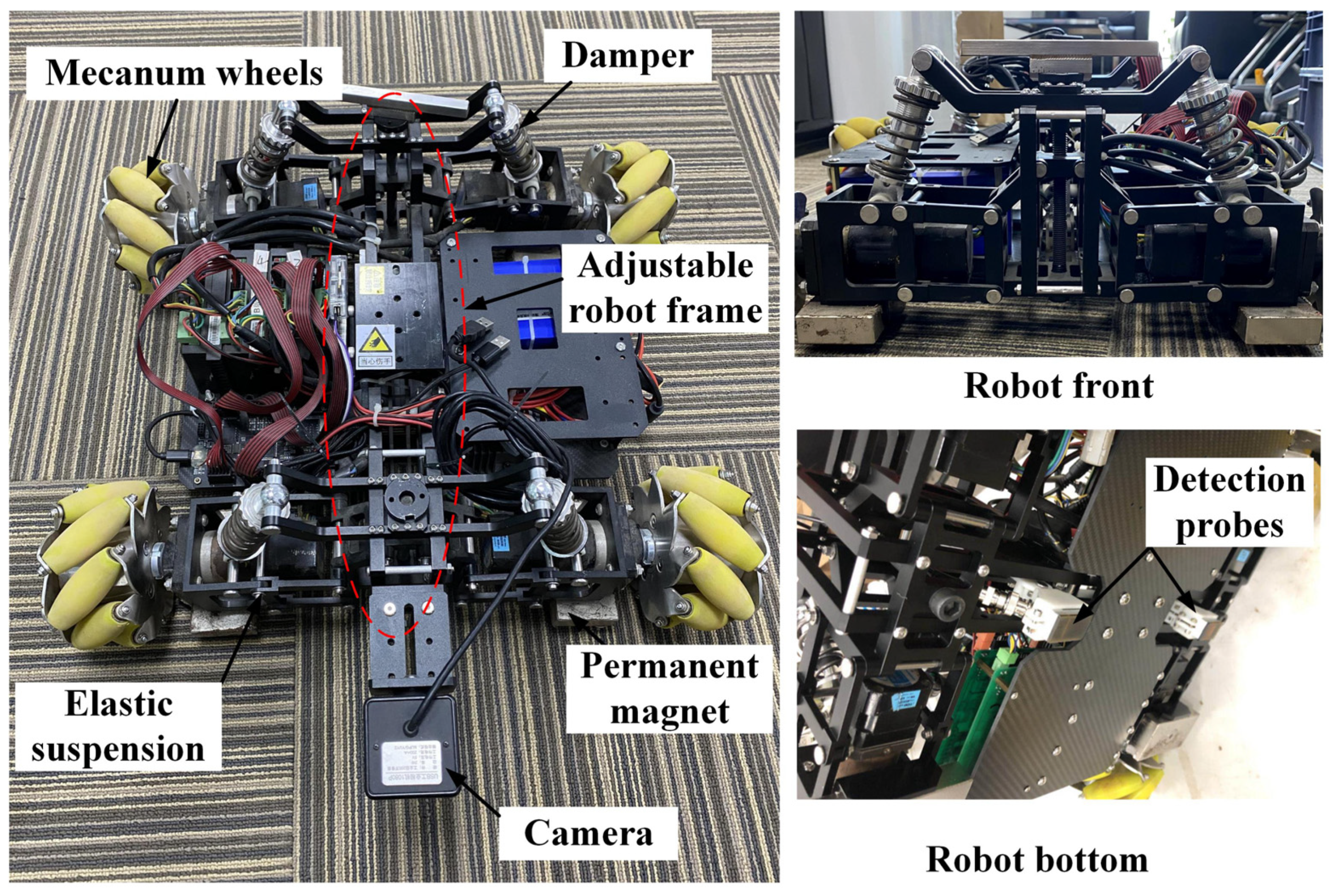
According to the results of preliminary tests [25,26,27], an upgraded inspection robot for weld seam identification and tracking was designed. As shown in Figure 2, the inspection robot is composed of four mecanum wheels, four elastic suspensions, four dampers, four permanent magnets and an adjustable robot frame. A camera is installed at the front of the robot for weld seam identification and two detection probes are installed at its bottom for defect detection in the weld seams.

The inspection robot should provide a sufficient adsorption force at any position of the tank, especially on the vertical and bottom surfaces. On the tank surfaces of 0° and 90°, the adsorption force $F_N$ should satisfy the following formulas, respectively: $\mu F_N>G_t$ and $\mu F_N>G_t$, where $G_t$ is the gravity of the robot and $\mu$ is the frictional coefficient of wheels. Compared to electromagnetic adsorption or other means, permanent magnet adsorption can provide greater adsorption force, save energy and avoid the risk of falling. The robot with mecanum wheels has omnidirectional movement ability, which reduces the risk and energy consumption of swerving and turning around when the robot climbs on the spherical tank.

The inspection robot adopts four-wheel independent elastic suspensions and the adjustable robot frame, which can adjust the inclination of mecanum wheels to be adapted to working surfaces with different curvatures. Each elastic suspension includes an independent damping mechanism, which reduces the instability of the robot and absorbs excess vibration energy. Meanwhile, four permanent magnets can provide sufficient adsorption force to ensure the smooth climbing of the robot on spherical tank surfaces.

When climbing on spherical tanks, the inspection robot has two states: the normal climbing state and the obstacle-surmounting state. The obstacle-surmounting capacity is an important performance of the robot. On the working surface of spherical tanks, the height of weld seams is about 3–4 mm. The robot needs to surmount weld seams during the running process. Dampers installed on independent suspensions can automatically adjust the robot’s posture for smoothly surmounting weld seams. The mechanical structural design of the robot can meet the operational requirements on spherical tanks.

The relevant parameters of the inspection robot with mecanum wheels are shown in

Table 1. Performance and parameters of the inspection robot.

Symbols	Meanings	Unit	Quantitative Values
$M_G$	Self-weight	kg	13.75
$M_l$	Maximum payload	kg	10
$V_{\max }$	Maximum velocity	m/s	0.2
$F_N$	Adsorption force	N	204
$h_m$	Obstacle-surmounting height	mm	5
$T$	Working time	min	120

. The self-weight of the robot is reduced from 20 kg to 13.75 kg, and the robot payload capacity is increased from 5 kg to 10 kg. To benefit from improved elastic suspensions, the adsorption force of the robot is increased from 180 N to 204 N, and the obstacle-surmounting height is also increased to 5 mm. The maximum climbing velocity is set as 0.2 m/s, and the maximum continuous working time about is 120 min. The improvement in the performance of the inspection robot could increase the application scope and reduce operational risks.

2.2. Robotic System Composition

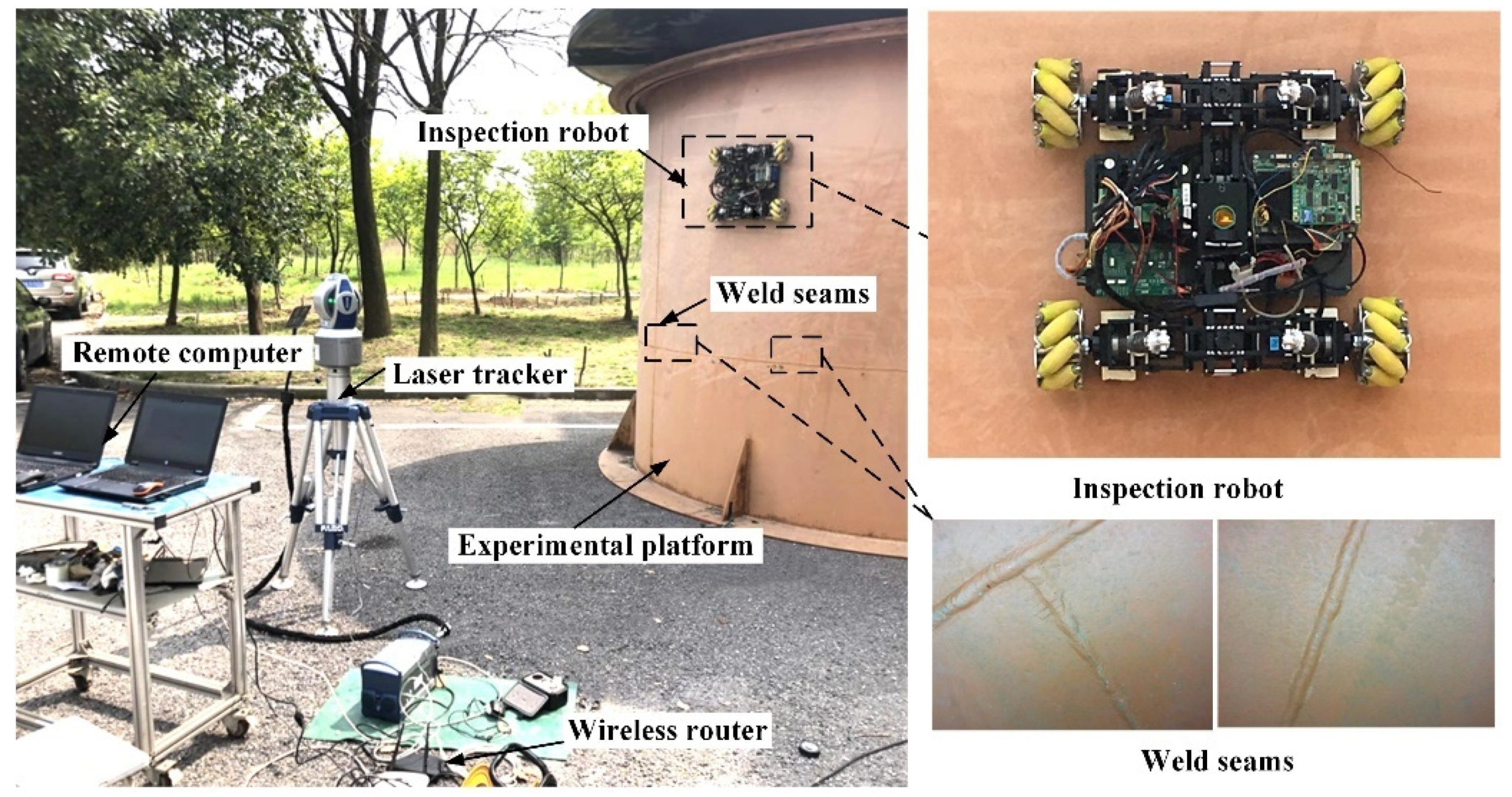
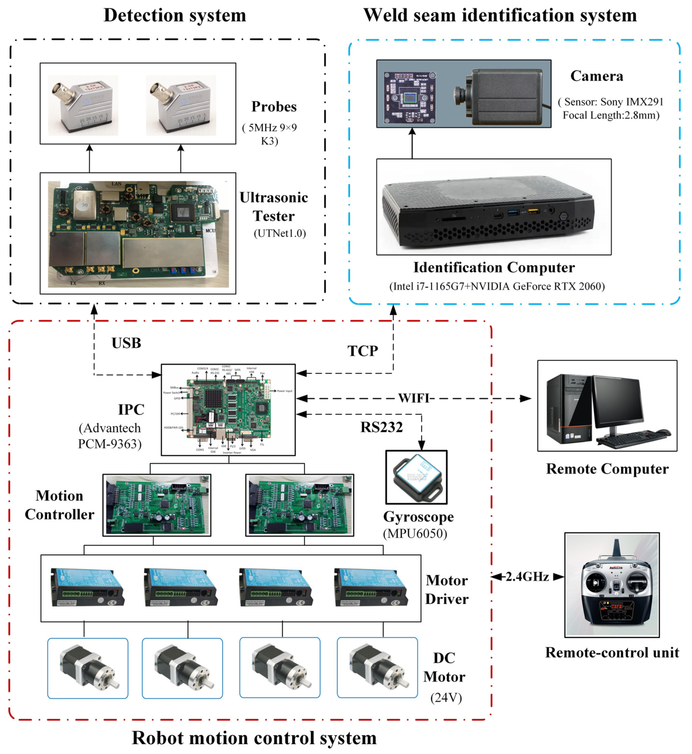
The weld seam identification and tracking system of the inspection robot is a composite system and its main functions include weld seam identification, path calculation, motion control and data transmission. As shown in Figure 3, the robotic system includes the following subsystems: robot motion control system, weld seam identification system, detection system and remote computer. The robot motion control system mainly includes an industrial personal computer (IPC), motion controller, motor drivers, DC motors, a gyroscope and a remote control unit. It realizes the movement function of the robot, position adjustment and remote control. The weld seam identification system is used to identify weld seams and calculate seam path, including an identification computer (GPU RTX 2060) and an industrial camera. The detection system is an additional device of the robot, and the defect detection of weld seams is performed by ultrasonic probes. The remote computer is connected to the robot through a wireless router for data analysis and storage.

Problems that can be solved by the robotic system include:

(1)

Accurate identification of weld seams by machine vision;

(2)

Weld path extraction and fitting;

(3)

Weld seam tracking by the inspection robot.

3. Weld Seam Identification

3.1. Weld Seam Images

In the field of computer vision, image processing is a general and fast method. Image processing can extract feature information in a certain image or identify lines that are distinguished in colors. However, in some complex environments, where the acquired images have similar colors (such as painted weld seams) or too much interference, it is difficult to obtain useful information through image processing. In the case of weld seams without obvious distinction, weld seams cannot be accurately identified and extracted by image processing. Even if some features are acquired, the path information is largely discontinuous, unclear and distorted [28].

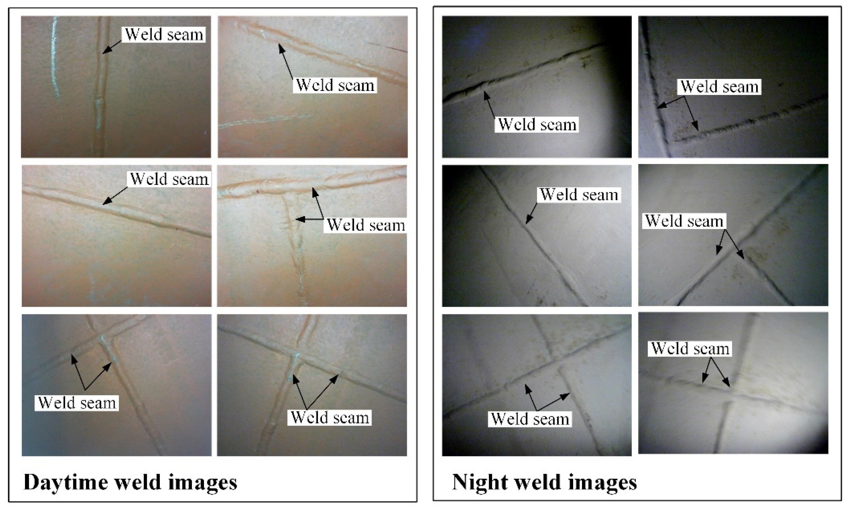
Real-time weld path tracking can make the inspection robot more automatic and intelligent. However, it is difficult to realize the weld seam identification and path line extraction with high-precision. After long-term work, the weld seams on spherical tank surfaces are covered by dirt and rust, which seriously affect identification accuracy. Weld seam images under the daytime and nighttime lighting conditions acquired by the inspection robot are shown in Figure 4. According to distribution characteristics, weld seams on tank surfaces include transverse weld seams, longitudinal weld seams, diagonal weld seams, crossed weld seams, etc. Different weld seam categories increase the difficulty in fitting weld paths. Due to the small distinction between weld seams and the surrounding feature identification by image processing is usually incomplete and it is difficult to extract the seam path information. Some image processing techniques [28], such as edge detection algorithms and digital morphology, have been tested to extract weld seam path lines, but the extraction results are not satisfactory.

3.2. Weld Identification Workflow

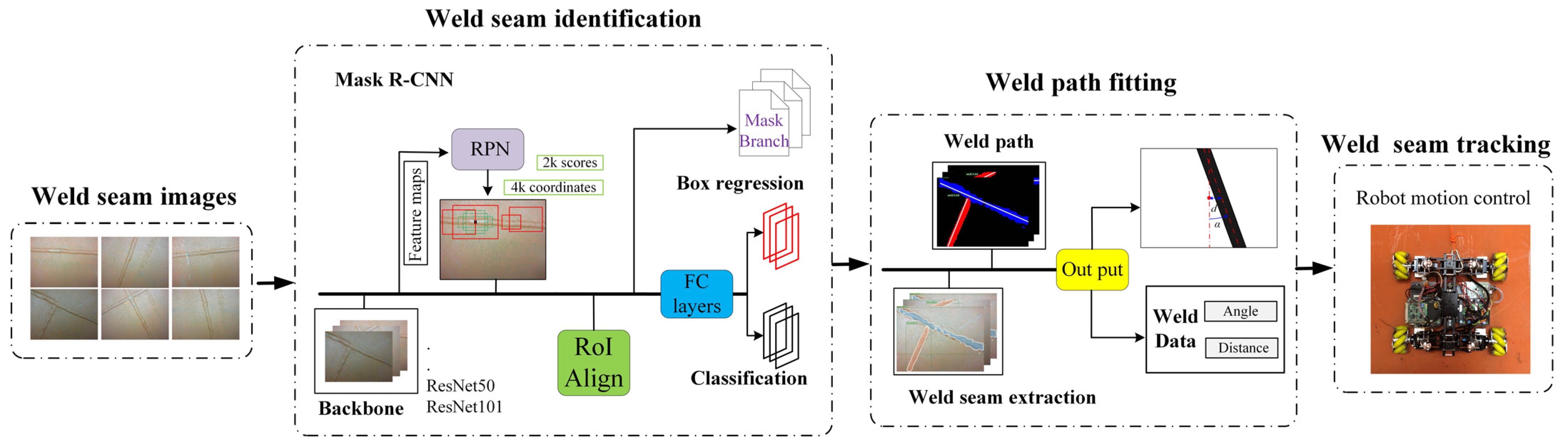
Figure 5 shows the workflow of weld seam identification and tracking, which is divided into four steps. Firstly, the weld images are captured by the camera; secondly, weld seams in images are identified by deep learning networks; thirdly, seam paths are extracted and fitted; finally, the robot is controlled to track weld paths based on path information. The purpose of the deep learning networks we used is to accurately segment weld seams. The ultimate goal is to extract weld seams and output path information.

In the initial phase, the camera of the robot acquires the images of the local environment. Subsequently, a Mask R-CNN model is used to identify weld seams from images and perform instance segmentation. After identifying weld seams, weld path lines are extracted and fitted through Hough transform and image processing. Here, the position parameters of weld paths are estimated, including drift angle $\alpha$ and offset distance $d$. $\alpha$ is the inclination angle of the robot relative to the chosen weld seam and $d$ is the shortest distance from the path center line to the image center. These two parameters directly reflect the direction angle and climbing velocity of the robot. Finally, the inspection robot continuously changes its movement position to automatically track the chosen weld seam.

3.3. Networks Model

Mask R-CNN is a deep learning mode based on CNNs [23]. It can accomplish the segmentation of weld seams in images. Mask R-CNN performs well in weld seam identification in terms of accuracy and time, which can meet the requirements of the inspection robot. The process of Mask R-CNN for weld identification mainly includes: backbone networks, regional proposal networks (RPN), RoIAlign layers, classification, bounding-box regression and mask generation.

In the beginning, a series of CNN layers (such as VGG19, GoogLeNet [29], ResNet50 [30] and ResNet101) are used to extract feature maps. Deeper CNNs can extract deeper features of weld images, but they ignore the features of small-sized objects. At this stage, feature pyramid networks (FPN) [31] are used to fuse the feature maps from the bottom layer to the top layer to fully utilize the features at different depths. For example, in ResNet50-FPN, the feature map used is C2–C5.

The feature map processed by the backbone networks will be passed into RPN. The purpose of RPN is to recommend a region of interest (RoI) and it is a fully convolutional network. RPN takes weld images as the input and uses nine anchors of different sizes to extract the features of original images. RPN outputs a set of rectangular object proposals, and each region proposal has a suggested score. The anchor sizes have three categories: 128 × 128, 256 × 256 and 512 × 512. There are three kinds of proportional relationships: 2:1, 1:2 and 1:1.

Each sliding window (9 anchors) is mapped to a lower-dimensional feature, which is fed into two sibling fully-connected layers: a box-regression layer and a box-classification layer. At each sliding-window location, RPN simultaneously predicts multiple region proposals and the number of maximum possible proposals for each location is denoted as $k$. In the stage of RPN, by encoding the coordinates of $k$ boxes, the regression layer gives $4k$ outputs, and the classification layer outputs $2k$ scores (objective scores or non-objective scores) to estimate the probability for $k$ proposals.

Due to the different sizes of the region proposals obtained by RPN, these obtained regional proposals are sent to the non-quantization layer for processing, which is called RoIAlign. RoIAlign uses bilinear interpolation instead of quantization operations to extract fixed-size feature maps from each RoI (for example, 7 × 7). There is no quantization operation in the whole process. In other words, the pixels in the original image are completely aligned with the pixels in the feature map, and there is no deviation. In this way, the detection accuracy is improved, and the instance segmentation process is simplified.

Mask R-CNN finally outputs three branches: classification, bounding-box regression and mask prediction. After the RoIAlign layer, on the one hand, the RoI is fed into two fully connected layers for image classification and bounding box regression. The classification layer determines the category of weld seams. The bounding-box regression layer refines the location and size of the bounding box. On the other hand, pixel-level segmentation of weld seams is acquired through FCN. FCN uses convolutional layers instead of fully connected layers for pixel-to-pixel object mask prediction. The mask prediction branch uses FCN to segment objects in the image by pixels and has a $K{m}^2$-dimensional output for each RoI ($K$ is the number of categories). In the dataset for the identification of weld seams, the number of categories was 2 (including background and weld seams), the network depth of the classification layer and regression layer was 2, and output network size of the mask prediction branch was $28\times 28\times 2$ pixels.

3.4. Loss Function

Weld seam images are segmented by Mask R-CNN. There are three output layers: the classification layer, bounding-box regression layer and mask branch. During the training process, the relevant variables and their meanings are shown in

Table 2. Variables and meanings in the loss function.

Symbols	Meanings
$L$	Total loss
$L_{cls+box}$	Sum of classification loss and bounding-box loss
$L_{mask-branch}$	Mask branch loss
$L_{cls}$	Classification loss
$L_{box}$	Bounding-box loss
$L_{mask}$	Average binary cross-entropy loss
$N_{cls}$	Number of corresponding anchors
$N_{reg}$	Number bounding boxes
$i$	Anchor index
${\rho }_i$	$\mathrm{Predicted}\mathrm{classification}\mathrm{probability}\mathrm{of}\mathrm{anchor}i$
${\rho }_i^{*}$	$\mathrm{Ground}\text{-}\mathrm{truth}\mathrm{label}\mathrm{probability}\mathrm{of}\mathrm{anchor}i$$;{\rho }_i^{*}$ is 1 for the positive anchor and 0 for the negative anchor
${\tau }_i=\left({\tau }_x,{\tau }_y,{\tau }_w,{\tau }_h\right)$	Difference between the prediction bounding box and the ground-truth label box in four parameter vectors (horizontal coordinate, vertical coordinate, width and height)
${\tau }_i^{*}=\left({\tau }_x^{*},{\tau }_y^{*},{\tau }_w^{*},{\tau }_h^{*}\right)$	Differences between the ground-truth label box and the positive anchor in four parameter vectors
${\lambda }_i$$,{\gamma }_i$	Hyper-parameters to balance the training losses of the regression and mask branch

. The total loss function is defined as:

$$L=L_{cls+box}+L_{mask-branch}$$

(1)

$$L_{cls+box}=L_{cls}+L_{box}=\frac{1}{N_{cls}}{\displaystyle \sum _i{L}_{cls}}\left({\rho }_i,{\rho }_i^{*}\right)+{\lambda }_1\frac{1}{N_{reg}}{\displaystyle \sum _i{\rho }_i^{*}}{L}_{reg}\left({\tau }_i,{\tau }_i{}^{*}\right)$$

(2)

Classification loss $L_{cls}$ can be defined as:

$$L_{cls}\left({\rho }_i,{\rho }_i^{*}\right)=-\log {\rho }_i^{*}{\rho }_i$$

(3)

Bounding-box loss $L_{box}$ is defined over a tuple of true bounding-box regression targets:

$$L_{reg}{}_{}\left({\tau }_i,{\tau }_i^{*}\right)={\mathrm{smooth}}_{L1}\left({\tau }_i^{*}-{\tau }_i\right)$$

(4)

$${\mathrm{smooth}}_{L1}(x)=\{\begin{array}{cc}0.5x^2& ,\mathrm{if}\left|x\right|<1\\ \left|x\right|-0.5& ,\mathrm{otherwise}\end{array}$$

(5)

Mask branch loss $L_{mask-branch}$ is defined as:

$$\begin{array}{ll}{L}_{mask-branch}& =L_{mask-branch}\left({\rho }_i,{\rho }_i{}^{*},{\tau }_i,{\tau }_i{}^{*},{\sigma }_i,{\sigma }_i{}^{*}\right)\\ & =\frac{1}{N_{cls}}{\displaystyle \sum _i{L}_{cls}}\left({\rho }_i,{\rho }_i{}^{*}\right)+{\lambda }_2\frac{1}{N_{reg}}{{\displaystyle \sum _i{\rho }_i}}^{*}{L}_{reg}\left({\tau }_i,{\tau }_i{}^{*}\right)+{\gamma }_2\frac{1}{N_{\mathrm{mask}}}{\displaystyle \sum _i{L}_{\mathrm{mask}}}\left({\sigma }_i,{\sigma }_i{}^{*}\right)\end{array}$$

(6)

$L_{mask}$ is defined as the average binary cross-entropy loss by used a per-pixel sigmoid. The definition of $L_{mask}$ allows the network to generate masks for every category without competition.

3.5. Training

During the training phase of Mask R-CNN, 2281 weld seam images at different angles were collected (more images might have the better effect). The image size was fixed at 320 × 240. In the collected images, 1500 images were used as the training dataset; 500 images were used as the verification set; and 281 images were used as the testing set. These dataset images were labelled and processed in advance. Some data augmentation methods, such as random flip, random crop, color jitter and noise addition, were used to extend the dataset. Image transformations and noise addition were beneficial to avoid overfitting. After data augmentation (24 types), the number of weld seam images in the training set, validation set and test set were 37,500, 12,500 and 7025, respectively. 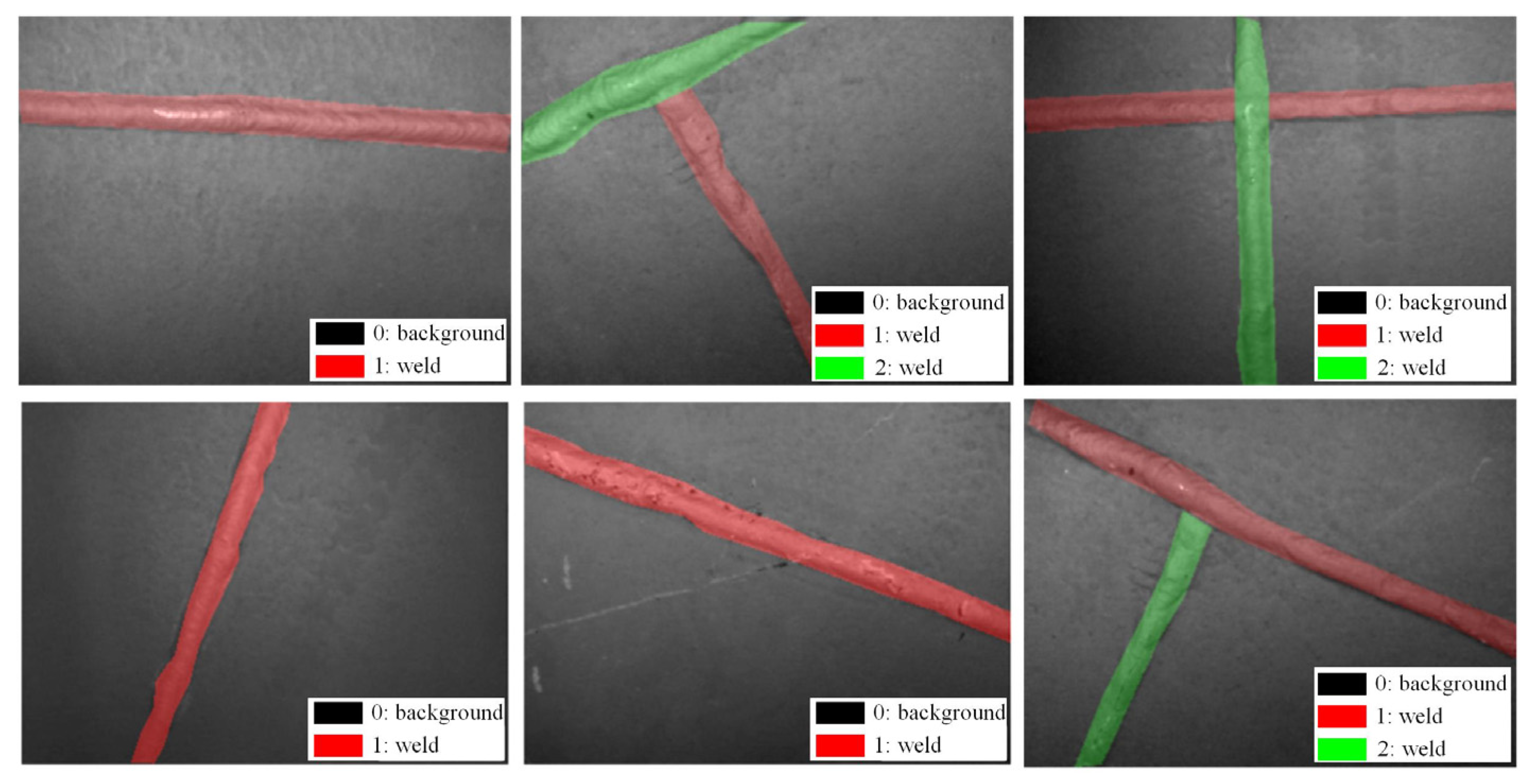Figure 6 visualizes results of the weld seam dataset. Regarding the label number, 1 (or 2) represents weld seams and 0 represents the background.

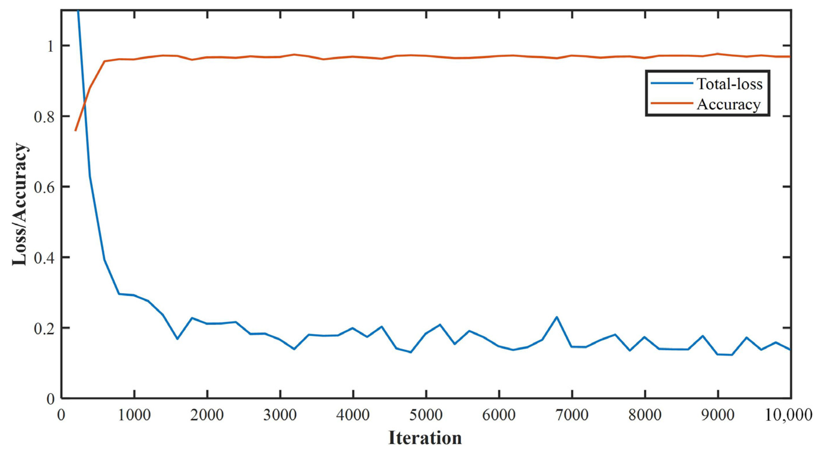
The pre-trained Mask R-CNN weight was inherited from the COCO dataset and the backbone network was ResNet101 + FPN. The number of categories was 2 (background and weld). The model output the category scores, bounding boxes and masks of weld seams for each input image after training. The training parameters were set as follows: the initial learning rate of the network was 0.001; the weight attenuation coefficient was 0.0005; the momentum coefficient was 0.85. During the deep learning training process of the weld seam dataset, the loss function and accuracy curve changes as shown in Figure 7. After 10,000 iterations, the training loss function curve stabilizes at 0.15–0.2, and the accuracy of the network model is greater than 0.97. Comparing the learning effect of 3000, 5000 and 8000 iterations, due to smaller weld images and the number of categories is only 2, the effect after 3000 iterations is already good and after 5000 times is basically stable.

4. Weld Path Tracking

4.1. Path Selection Problem

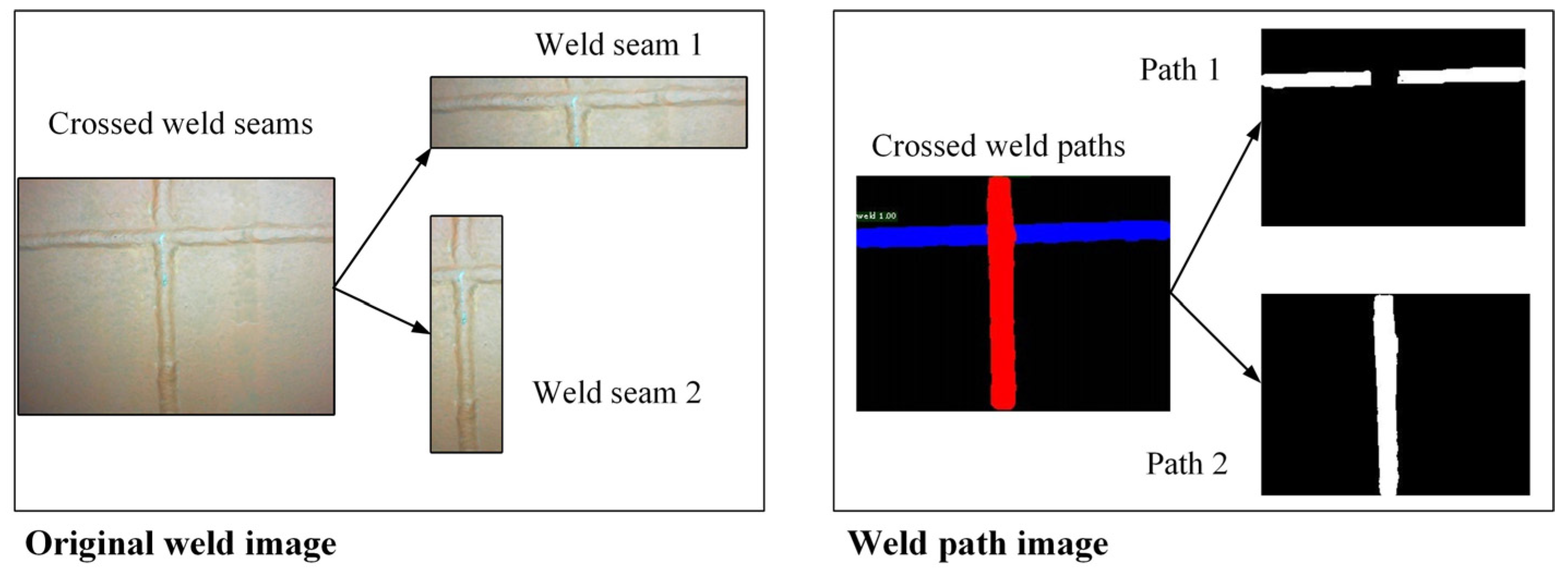
Since weld images not only include a single weld seam (such as transverse and longitudinal weld seams) but sometimes include multiple weld seams (such as T-shape and crossed weld seams). When there are multiple weld seams in an image, the following possibilities exist in the weld path extraction stage:

(1)

Extract the path of weld seam 1

(2)

Extract the path of weld seam 2

(3)

Extract one wrong path

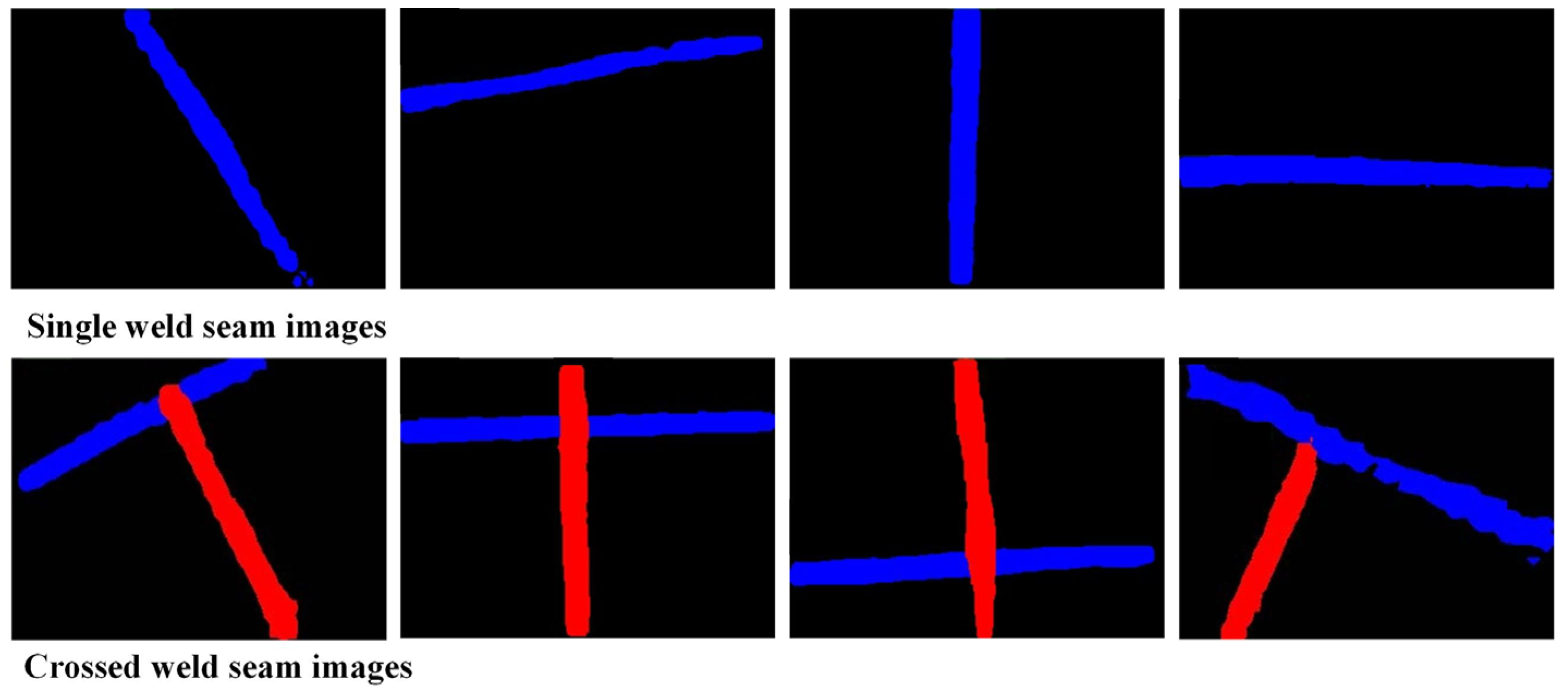
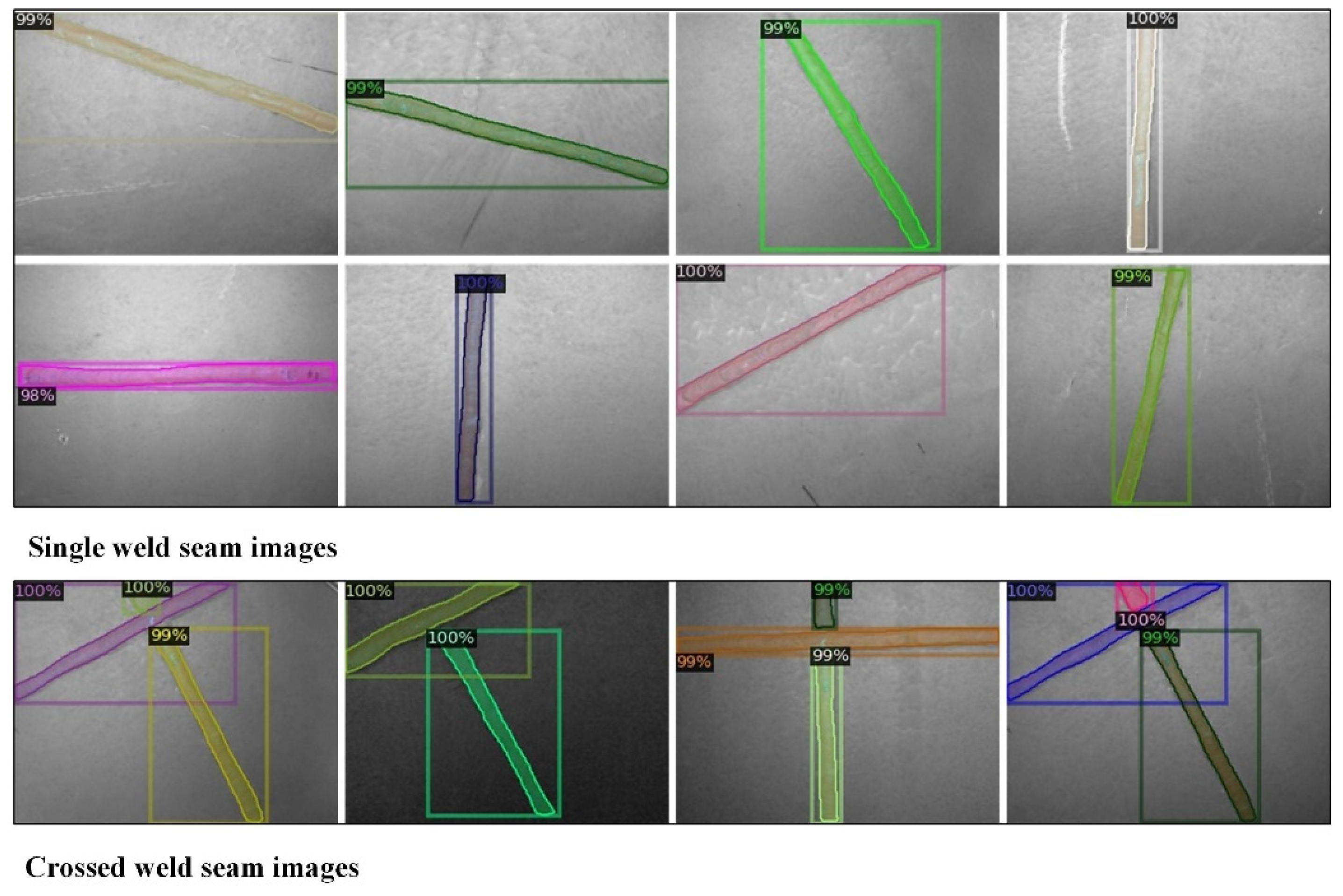
As shown in Figure 8, in order to avoid the interference of multiple paths, the acquired weld seams are identified and distinguished by different colors, and the centerline of each weld seam is fitted separately. If there are T-shape or crossed weld seams in the weld images, multiple weld seams are segmented.

In general, the crossed weld seam is considered to be a special welding joint, so the crossed weld seam is defined as a combination of two weld seams. Therefore, the optimal weld path can be efficiently processed. In the weld identification phase, Mask R-CNN has a more obvious advantage in segmenting multiple weld seams; these weld seams are distinguished by different color pixels.

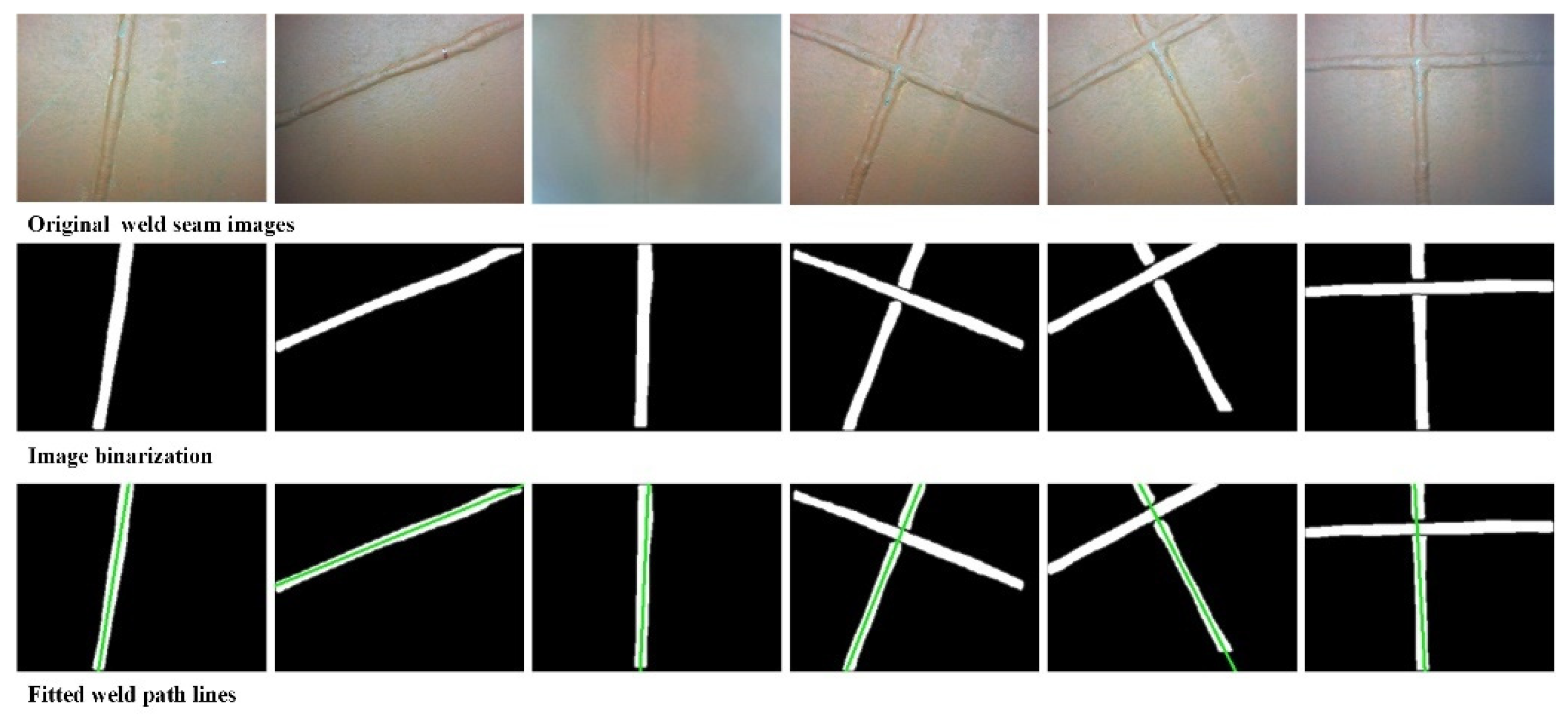
4.2. Weld Path Fitting

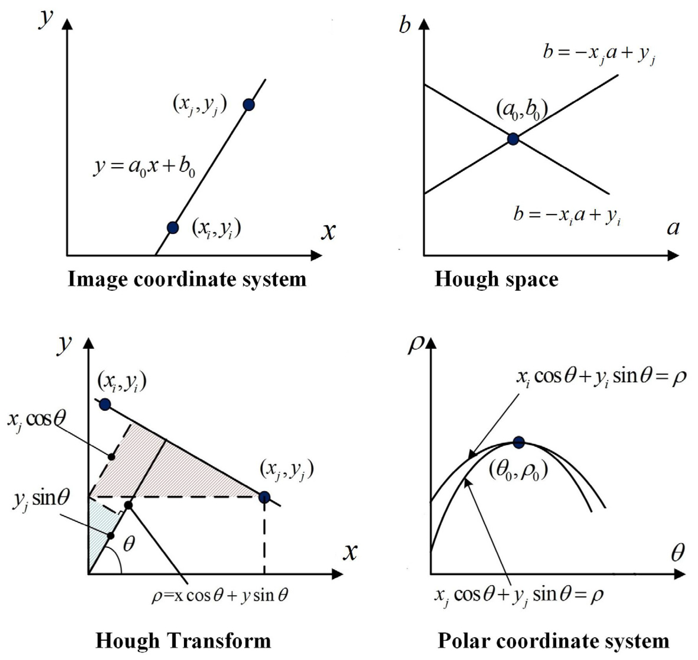
Binarized images of weld paths are generated through image processing, and image erosion and filtering are also executed. Hough transform is used to fit the path line of a single weld seam. In the image coordinate system $\left(x,y\right)$, the path line of the weld seam can be supposed as:

$$y=a_{0}x+b_0$$

(7)

After mapping the line to Hough space $\left(a,b\right)$, the line equation can be expressed as:

$$b_0=-x{a}_0+y$$

(8)

Each line in the image space can be described as a point in the Hough space. As shown in Figure 9, point $\left(x_i,y_i\right)$ and point $\left(x_j,y_j\right)$ correspond to two straight lines in Hough space, respectively:

$$\{\begin{array}{l}b=-x_{i}a+y_i\hfill \\ b=-x_{j}a+y_j\hfill \end{array}$$

(9)

The straight line equation can be converted into polar coordinate system $\left(\theta ,\rho \right)$:

$$x\cos \theta +y\sin \theta =\rho$$

(10)

So, the straight line equation of the weld path can be expressed as:

$$y=\frac{-\cos \left({\theta }_0\right)}{\sin \left({\theta }_0\right)}x+\frac{{\rho }_0}{\sin \left({\theta }_0\right)}$$

(11)

$a_0$ and $b_0$ can be expressed as:

$$\{\begin{array}{l}{a}_0=-\cos \left({\theta }_0\right)/\sin \left({\theta }_0\right)\\ b_0={\rho }_0/\sin \left({\theta }_0\right)\end{array}$$

(12)

In the polar coordinate system, point $\left({\theta }_0,{\rho }_0\right)$ represents a straight line in the image coordinate system. The number of curves passing through point $\left({\theta }_0,{\rho }_0\right)$ can represent the quantity of points in a straight line in the image coordinate system. The straight lines in the image coordinate system are converted into the points in the polar coordinate system, and the straight line with the most points in the image coordinate system can be determined as the weld seam path line.

Through Hough transform, multiple straight line functions in the weld image can be fitted. The line with the maximum linear length is selected as the weld path line. There is a slight deviation between the solved path line and the actual path centerline, but it can meet the requirement of robot tracking.

According to the weld path line parameters $a_0$ and $b_0$, the drift angle $\alpha$ and offset distance $d$ of weld paths can be expressed as:

$$\{\begin{array}{l}\alpha =\frac{\mathrm{arc}\tan \left(-a_0\right)\cdot 180}{\pi }\\ d=\frac{x_c-b_0}{k}-y_c/2\end{array}$$

(13)

where $\left(x_c,y_c\right)$ is the center coordinate of weld line images.

4.3. Robot Kinematics

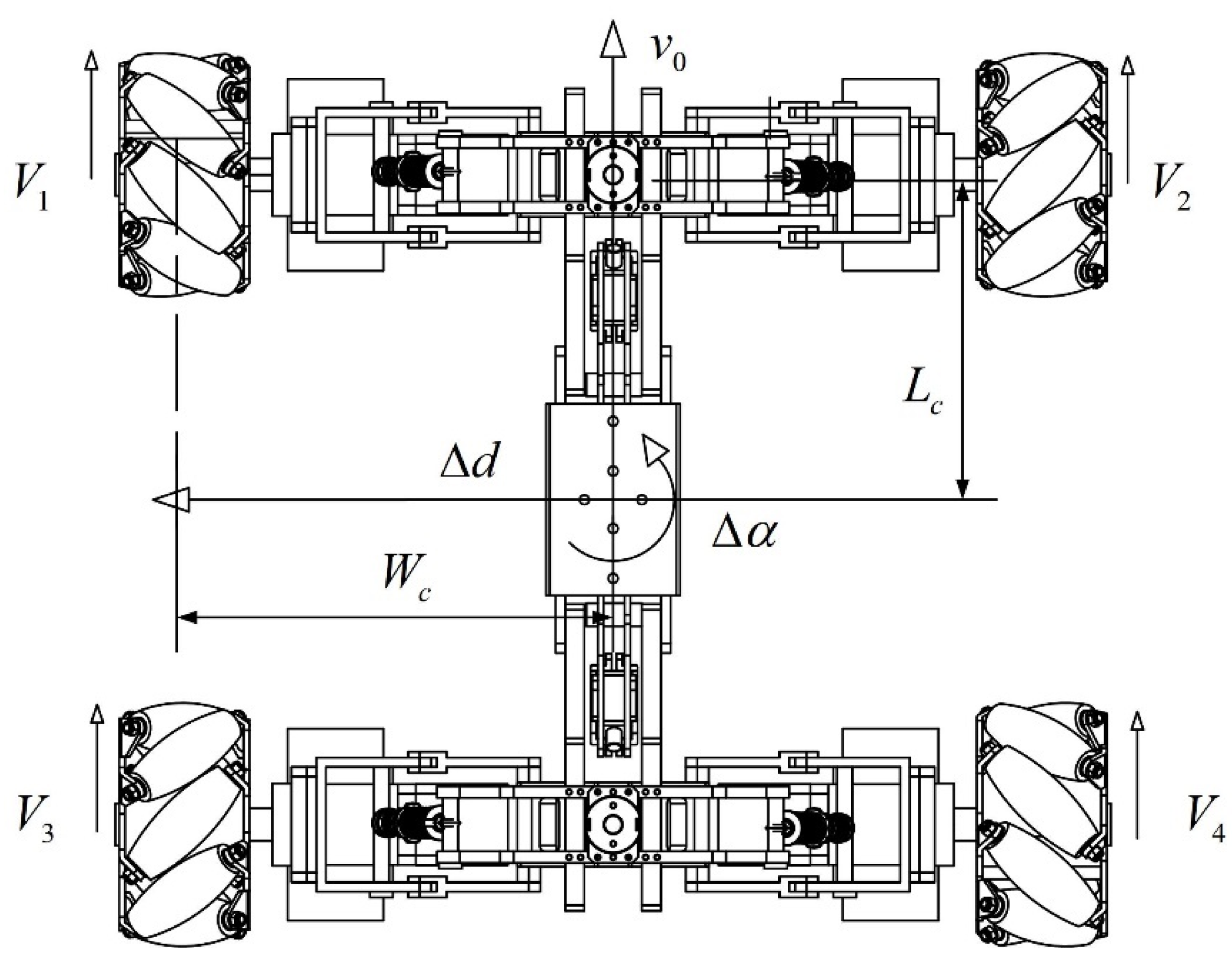
The inspection robot with mecanum wheels can achieve omnidirectional movement. Based on elastic suspensions and the adjustable robot frame, the robot can move flexibly on curved surfaces, so the weld seam tracking on spherical tanks can be simplified as a plane adjustment motion. In this process, the robot continuously corrects drift angle $\alpha$ and offset distance $d$ to climb forward along welding seams.

As shown in Figure 10, assuming that the robot forward velocity is $v_0$, the rotation angular velocity and lateral velocity to be adjusted are $\Delta \alpha$ and $\Delta d$, respectively. Then the inverse kinematics equation of tracking movement is:

$$\left[\begin{array}{c}{\dot{\theta }}_1\\ {\dot{\theta }}_2\\ {\dot{\theta }}_3\\ {\dot{\theta }}_4\end{array}\right]=\frac{1}{R_c}\left[\begin{array}{ccc}1& -\cot {\beta }_c& -(W_c+\cot {\beta }_c\cdot L_c)\\ 1& \cot {\beta }_c& W_c+\cot {\beta }_c\cdot L_c\\ 1& -\cot {\beta }_c& W_c+\cot {\beta }_c\cdot L_c\\ 1& \cot {\beta }_c& -(W_c+\cot {\beta }_c\cdot L_c)\end{array}\right]\left[\begin{array}{c}{v}_0\\ \Delta d\\ \Delta \alpha \end{array}\right]$$

(14)

$$V_i=R{\dot{\theta }}_i\left(i=1,2,3,4\right)$$

(15)

where $V_i$ and $\dot{\theta }i$ are the velocities and angular velocities of four mecanum wheels, respectively. $W_c$ and $L_c$ are the half-width and half-length of the robot frame. $R$ is the radius of the mecanum wheels and ${\beta }_c$ represents the angle between the wheel roller and the wheel axis. Substituting with robot design parameters, the Jacobian matrix (defined as $K_c$) of inverse kinematics of the robot is:

$$K_c=\frac{1}{0.0635}\left[\begin{array}{ccc}1& -1& -0.788\\ 1& 1& 0.788\\ 1& -1& 0.788\\ 1& 1& -0.788\end{array}\right]$$

(16)

5. Experiments and Results

As shown in Figure 11, the experimental platform is a cylindrical tank with a diameter of 4000 mm, a height of 2800 mm and a thickness of 10 mm. Weld seams are distributed on the surface of the experimental tank for identification and tracking by the robot. The laser tracker was used to record the running position of the inspection robot.

5.1. Weld Seam Identification Experiments

Figure 12 shows weld seam identification results by the robot. From the perspective of identification effect, accurate outline descriptions of weld seams have been generated with over 98% identification probability. Generated pixel-level masks can cover weld seams, which is beneficial for extracting and fitting weld paths.

Table 3. Box AP and mask AP of weld seam identification.

(%)	AP	AP50	AP75	APs	APm	APL
Box	78.947	96.193	90.802	nan	86.079	3.791
Mask	67.596	90.802	90.802	nan	71.252	0.000

shows the statistical data of weld seam box AP (bounding box AP) and mask AP. The average precision calculation formula is as:

$$AP={\displaystyle {\int }_0^{1}P}\left(r\right)dr$$

(17)

where $P$ and $r$ represent precision and recall of each image, respectively. Mask AP and box AP are 67.5% and 78.9%, respectively. Both AP₅₀ and AP₇₅ are greater than 90%. Results of AP_s, AP_m and AP_l show that the size of weld seams is mainly concentrated in the medium pixel size (32²–96²).

5.2. Weld Path Fitting Experiments

As shown in Figure 13, multiple weld paths are extracted using different colors. When the weld images are crossed weld seams, two weld path lines are fitted by dividing them into red and blue. Figure 14 shows image binarization and fitting results of weld paths. The robot can accurately fit path lines to estimate their positional parameters (drift angle and offset distance).

Figure 15 shows the deviations between the calculated values and the actual measured value of drift angle $\alpha$ and offset distance $d$. In deviation values of single weld seams, the average deviation of drift angle $\alpha$ between calculated paths and actual paths is 1.01°, and the maximum deviation is 2.78° (Figure 15a). The average deviation of offset distance $d$ is 2.21 pixels, and the maximum value is 5.57 pixels (Figure 15b). In terms of the deviation of crossed weld seams, the average and maximum deviations of drift angle $\alpha$ are about 0.87° and 2.37° (Figure 15c), and the average and maximum deviations of offset distance $d$ are 2.62 pixels and 7.83 pixels (Figure 15d). These deviations are generally kept at small values which have little effect on the weld path tracking by the robot.

Table 4. Time consumption of weld seam identification and processing.

Image Number	1	2	3	4	5	…	196	197	198	199	200	Mean Time (s)
Time0 (s)	0.172	0.236	0.226	0.176	0.142	…	0.155	0.163	0.161	0.156	0.156	0.162
Time1 (s)	0.007	0.007	0.003	0.007	0.003	…	0.006	0.007	0.006	0.006	0.007	0.006
Time2 (s)	0.147	0.181	0.202	0.144	0.130	…	0.129	0.133	0.131	0.131	0.130	0.137
Time3 (s)	0.019	0.049	0.021	0.023	0.009	…	0.019	0.023	0.023	0.019	0.019	0.018

Note: Time₀ = total time; Time₁ = loading time; Time₂ = identification time; Time₃ = image processing time.

shows the time consumption of weld seam real-time identification and processing, which mainly includes image loading loss time, deep learning identification time, image processing time and total time. In the process of continuous weld seam identification, the total processing time of each image is kept between 0.15 s and 0.18 s, the average time of the deep learning network of each image is 0.137 s, the average image loading loss time is about 0.006 s and the average image processing time is about 0.018 s.

In the real-time weld seam identification, the robotic system can output five sets of path data (drift angle and offset distance) in one second. Due to the low running velocity of the robot, it can meet the automated inspection work. Weld seam identification speed can be accelerated by optimizing deep learning identification time and clearing the loss time of loading images.

5.3. Robot Tracking Experiments

According to the imaging ratio of the camera, the actual offset distances between weld paths and the inspection robot were calculated. Based on the robot kinematics, the rotation velocities of four motors were adjusted, and the attitude and position of the robot were continuously changed to track the identified weld seam. Due to the drive mode of mecanum wheels, the robot could achieve omnidirectional movement without frequently changing its heading angle. In robot tracking experiments, when the drift angle was over ±3°, the climbing robot would rotate to correct its heading angle.

Figure 16 shows the drift angles and offset distances of robot while tracking the identified weld seams. The robot can successfully correct its angle and velocities to track weld seams. The maximum drift angle and offset distance were about 3° and 10 mm, respectively. The accuracy of tracking weld seams could meet the operational requirements of the inspection robot.

6. Conclusions

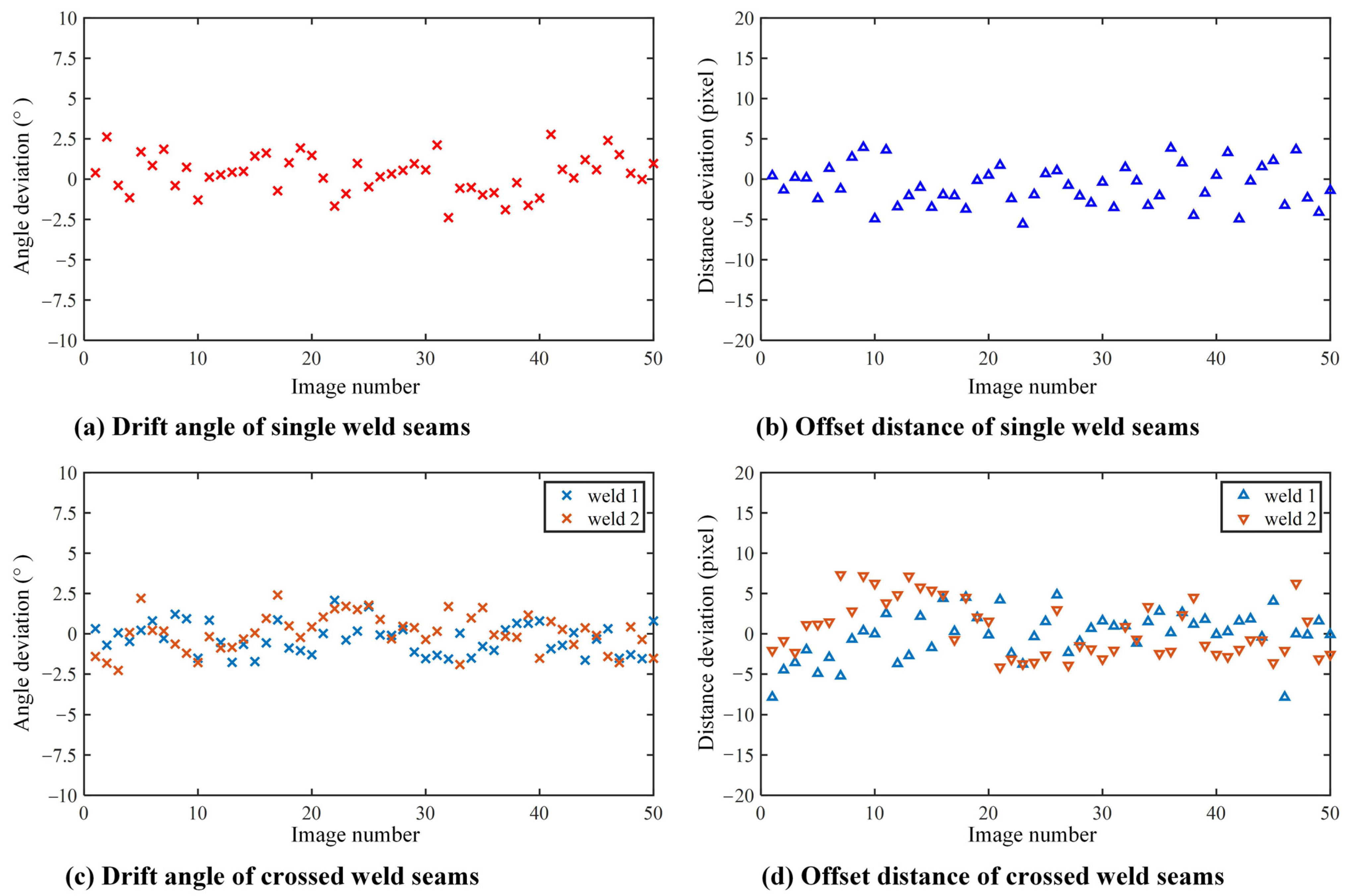
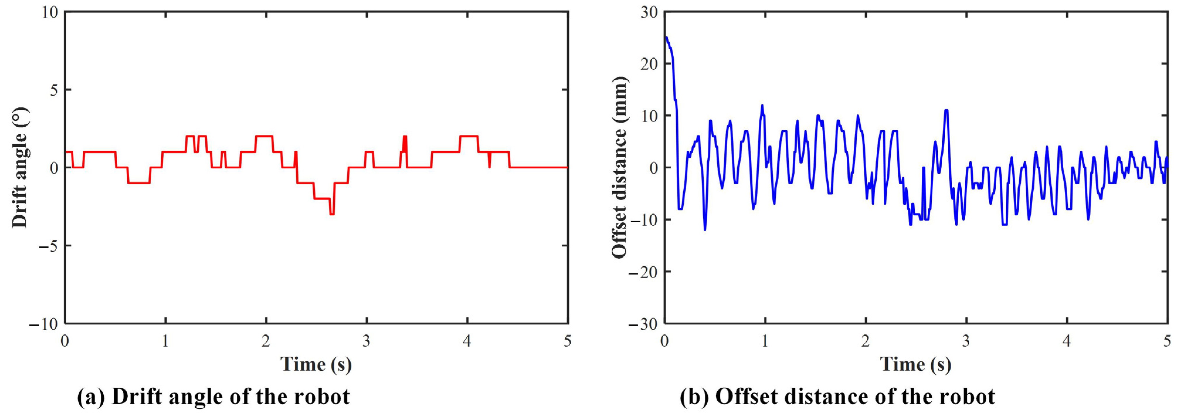
In this study, an intelligent inspection robotic system based on deep learning was developed to achieve the weld seam identification and tracking. The inspection could complete the segmentation of weld images and output the masks of weld paths using Mask R-CNN. Deep learning weld seam identification makes up for the low accuracy of image processing. By using specific colors to distinguish multiple weld seams, possible errors in the fitting weld path can be avoided. The real-time test results indicated the deep learning model had higher accuracy in weld seam identification, and the average processing time of each image was about 180 ms. Weld path fitting experiments were carried out to test weld path extraction deviation. The maximum deviations of drift angle $\alpha$ and offset distance $d$ were within 3° and 8 pixels, respectively. The results of robot tracking experiments demonstrated the inspection robot could accurately track weld seams, with a maximum tracking deviation of 10 mm.

The further training and adjusting of the network structure will be explored to speed up processing. In the construction process of the entire robotic system, due to the combination of multiple methods and algorithms, optimizing the system composition and connection is also one of our priorities in the future. In terms of engineering applications, this robotic system can meet the basic operational and inspection requirements and the robot performance will be promoted in further research.