Abstract
In this paper, the multiple autonomous underwater vehicles (AUVs) task allocation (TA) problem in ocean current environment based on a novel reinforcement learning approach is studied. First, the ocean current environment including direction and intensity is established and a reward function is designed, in which the AUVs are required to consider the ocean current, the task emergency and the energy constraints to find the optimal TA strategy. Then, an automatic policy amendment algorithm (APAA) is proposed to solve the drawback of slow convergence in reinforcement learning (RL). In APAA, the task sequences with higher team cumulative reward (TCR) are recorded to construct task sequence matrix (TSM). After that, the TCR, the subtask reward (SR) and the entropy are used to evaluate TSM to generate amendment probability, which adjusts the action distribution to increase the chances of choosing those more valuable actions. Finally, the simulation results are provided to verify the effectiveness of the proposed approach. The convergence performance of APAA is also better than DDQN, PER and PPO-Clip.
1. Introduction
Recently, with the development of Autonomous Underwater Vehicle (AUV) technology [,], AUV has been widely applied in hunting [,], rescue [], detection [,] and other tasks [,,]. Compared with single AUV system, multiple autonomous underwater vehicles (AUVs) can be competent for more complex tasks []. Therefore, the problem of cooperation between AUVs has attracted wide attention. Among many cooperation problems, task allocation (TA) [] is critical for AUVs to perform tasks successfully. The description of the TA for a multi-AUV system in the ocean current is shown in Figure 1. If some soluble targets that can be denoted as drifted in the ocean current as a result of a transport ship accident, the surrounding AUVs denoted as need to collaborate to complete the task, that is rescuing the five targets immediately. The AUVs establish a temporary communication network, which can share the location of the targets as well as the location and speed of all AUVs, and the drifted targets to be salvaged when the total power of the nearby AUVs exceeds its weight. Besides, the AUVs are also required to consider the impact of the ocean current, energy consumption, the task emergency and avoid collisions with other AUVs. As a result, due to the tough environment, an optimal salvage strategy is needed to ensure that AUVs accomplish the task safely and quickly.
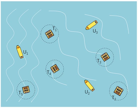
Figure 1.
The description of the TA for multi-AUV system.
At present, the methods for solving the TA problem with multi-constraints mainly include market-based method [], swarm intelligence method [] and reinforcement learning []. Although the market mechanism method can find the optimal solution, it has high requirements for real-time and communication ability of AUVs system. The swarm intelligence method can find acceptable solutions, but it has poor generalization ability and poor performance when dealing with unknown factors.
RL is an emerging field, which has been widely used in automatic control [], intelligent decision-making [], optimization [], scheduling [], etc. []. Using RL, AUVs can interact with the environment to obtain feedback signals from the environment by trial-and-error. Good behaviors will be enhanced, while bad behaviors will be weakened by signals, RL gradually learn the mapping between state and action to obtain the optimal policy with the maximum expected reward []. Q learning [] is one of the classical RL algorithms, which maps state actions into optimal value functions by using Q table. However, Q learning is affected by the curse of dimensionality, making it difficult to deal with problems that have high-dimensional continuous state space. In order to overcome the above-mentioned difficulties, deep Q network (DQN) is proposed, which uses neural networks to approximate the optimal value function [,]. Double Deep Q-Network (DDQN) [] is one of the most commonly used methods in DQN, which adopts the dual network structure. The current network is used for policy execution and the target network is used for policy evaluation, which solves the problem of overestimation in DQN.
Efficient use of samples is commonly used to improve the performance of traditional RL. The experience replay is used to learn existing samples by random sampling, which reduces the correlation between samples while improving sample efficiency []. However, each sample has a different influence on learning, and the effect of uniform sampling is very limited. Schaul et al. [] improved the traditional experience replay method by using TD-error to evaluate the importance of samples in the experience pool (EP), which improved the convergence of the importance sampling reinforcement learning. Horgan et al. [] presented shared prior experience replay so that RL can learn more data in distributed architecture training. Zhao et al. [] presented that learning high-return samples can effectively improve the convergence rate. In the algorithm, the authors took the sample sequence that has high-expectation rewards and TD-error as the basis of importance sampling to achieve good results. Zhang et al. [] proposed an adaptive priority correction algorithm to estimate the real sampling probability by evaluating the predicted TD error and the real TD error of the experience pool. Almost all the methods proposed above use either reward information or error generated by sample training to evaluate the importance. Others have suggested that sample information of different aspects can also improve performance. M. Ramicic and A. Bonarini [] improved the learning efficiency by using entropy to quantify the state space and carrying out importance sampling. Yang et al. [] constructed directed association graph (DAG) by using sample trajectory, and introduced episodic memory and DAG into traditional deep reinforcement learning (DRL) loss, which made DRL learn from different aspects and improved sample utilization rate.
The balance between exploration and exploitation remain challenging. Undirected space exploration makes the algorithm converge slowly, and excessive use of existing experience usually can only find a non-optimal policy. Pathak et al. [] proposed the curiosity mechanism to make space exploration more efficient. Zhu et al. [] used dropout regularization to predict the distribution of Q values and select actions in the form of maximizing the distribution of Q values. This method can effectively evaluate the learning of the environment and the trade-off exploration and exploitation in a non-stationary environment. Kumra et al. [] introduced a loss-adjusted exploration strategy to determine candidate actions based on Boltzmann distribution of loss estimation, ensuring the balance of exploration and exploitation. Other studies are based on the assumption of prior knowledge, which can be used to explore space more efficiently and improve performance. Shi et al. [] decomposed complex tasks into several sub-tasks and solved them separately, and used transfer learning to accelerate the learning of new tasks by combining the prior knowledge of sub-tasks. Pakizeh et al. [] constructed the Q tables by sharing knowledge among agents to improve the convergence.
Compared with the previous research results, the contributions of this paper are summarized as follows:
- (1)
- In the traditional methods, sample reuse is to extract experience by learning samples from replay buffer, and it cannot directly improve the quality of samples by guiding the behavior of policy. Furthermore, experience extracted from samples can improve the convergence, but the effect is related to the experience extraction. The algorithm we proposed can extract available information from samples and use the information directly in decisions. Our algorithm not overly dependent on training effect and can directly improve the sample quality.
- (2)
- The traditional methods based on sample reuse do not take the influence of exploitation on policy exploration into account. Automatic Policy Amendment algorithm (APAA) considers the balance between exploration and exploitation, and it uses entropy to evaluate the information extracted from samples, aiming to maintain certain exploration ability in action decision-making and avoid trapping into a non-optimal policy.
- (3)
- The traditional method based on importance evaluation generally evaluates the importance of samples with the expected reward, and does not consider the evaluation between samples with the same expected reward under environmental changes. To overcome the shortcoming, the subtask reward evaluation method is combined to distinguish the influence of the same reward value on policy under different situations.
The remainder of this paper is organized as follows. In Section 2, the environment of ocean current and the motions of AUVs are described. Section 3 introduces the related RL algorithm. Section 4 and Section 5 give the mathematical description of the reward function and the algorithm design, respectively. The simulation results and efficiency analysis are introduced in Section 6 and Section 7, respectively. Finally, a conclusion is presented in Section 8.
2. Problem Statement
2.1. Ocean Current Environment
Ocean current is the flow phenomenon of seawater in the ocean. The proper use of ocean current can help AUVs to save energy and more quickly accomplish the task, otherwise it may affect the completion of the task and even damage AUVs. The ocean current model is composed of several randomly distributed eddy equations, and it is defined in [] as
where is the central coordinate of the eddy, is the size of ocean current at , is the intensity coefficient of the eddy, and determines the rotation direction of the eddy. When is positive, the eddy rotates clockwise. Otherwise, the eddy rotates counter clockwise. is a sign function.
The ocean flow field is formed by the superposition of m eddies as
where is a random function.
2.2. AUVs Model
The multi-AUV system consists of AUVs, and be denoted by . For each , its model is defined as a quad tuple, in which , , , represent ’s position, maximum speed, capability for salvage and energy, respectively. We define the energy loss of in time t is proportional to the third power of its current propulsion velocity as
where k is the drag coefficient.
Let has eight discrete directions in its action space, which can be denoted by as shown in Figure 2. At time t, ’s position changes with its movement and the ocean current, and is calculated as
where . As shown in Figure 3.
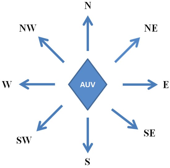
Figure 2.
Eight discrete directions of the AUVs in action space.
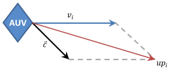
Figure 3.
Influence of ocean current on AUV’s direction.
2.3. Task Model
A task consists of targets, and the target i is defined as , and the target set is . For each , it can be represented by , , , , which denote the location, weight, emergency and complete sign of the target, respectively. We assume that the weight and emergency of these soluble targets decrease over time. The weight of at each time step t is expressed as
where is the function that taking the largest of two values and is the weight attenuation coefficient.
Then, the emergency of at time will be changed corresponding to , defined by
The task model requires AUVs not only to consider their own energy in the ocean current, but also to salvage the targets before dissolved in water as soon as possible. The distance between and in time t is calculated as
Let be the salvage radius of the targets. For each , which is not fully dissolved in water, it will be salvaged when the sum of capabilities of the AUVs in is greater than its weight, as shown in Figure 4. After that, is given by
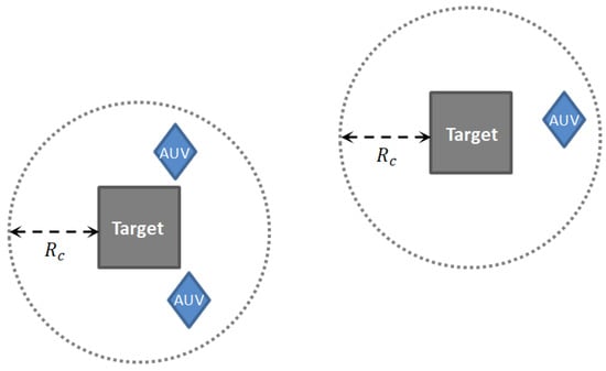
Figure 4.
AUVs cooperate to complete the task.
Not only the AUVs, but also the targets are affected by the ocean current, which will make them drift along with it, as shown in Figure 5. The movement model of the target is shown as
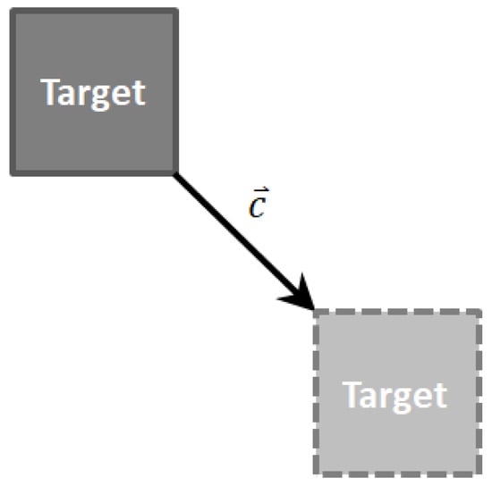
Figure 5.
Movement model of the target.
3. Background
Reinforcement Learning (RL)
RL can be described by Markov decision process (MDP), defined by the five tuples , in which S denotes the set of states, A is the set of actions, P denotes the state transition probability, R is a bounded reward function, and is the discount factor []. The agent interacts with the environment at each discrete time step , selects action a based on the current state , receives a reward and transfers to the next state according to probability , aiming to receive the maximum reward in one episode. The sum of the reward obtained by the policy is expressed as
In this paper, APAA we proposed based on the DDQN framework, which is a typical model of DRL, then it and some related algorithms are compared with APAA. DDQN, as one of the most commonly used variants of DQN, solves the overestimation of Q value. The target network is used to evaluate the optimal action of the current network, and the loss function is defined as
where is a current network for policy selection, and is a target network for policy evaluation. The two network usually synchronization after several iterations with the current network.
4. Model Design
4.1. State Model
Assume that each AUV has the information including the direction of the ocean current, all state information of itself, other AUVs, and all the targets. The state perceived by at time t is expressed as , in which represents the state of at time t, denotes the state of other AUVs at time t, represents the state of the targets at time t and is the current direction of the at .
4.2. Action Model
For each AUV, its action space is divided into eight directions including north, northeast, east, southeast, south, southwest, west and northwest. In each direction, the AUV can move at maximum speed or at 70% of maximum speed, and even remain stationary, that is, it does not perform any of its own movement, but only relies on the ocean current to change its position.
4.3. Reward Model
The reward an AUV received in a time step is composed of four parts, i.e., energy consumption, moving evaluation, collision detection and task completion.
- Energy consumption is determined by the AUV’s speed. The faster the AUV speed in each time step, the larger the energy consumption is, and the lower the reward value will be, the reward for the energy consumption is defined aswhere is the initial energy of , is the energy attenuation ratio at the maximum speed. The energy consumption decreases to 0 when the AUV moves only by ocean current, it will get the maximum energy consumption reward 0 in this situation.
- Moving evaluation is determined by the AUV whether it is closer to the nearest target than it was at the previous time step, the reward for the moving evaluation is defined as
- Collision detection is to judge whether an AUV collides with others. It will get a negative reward when colliding with others. The reward for the collision is defined aswhere is a small positive number, and it represents the minimum safe distance between AUVs to avoid collision, as shown in Figure 6.
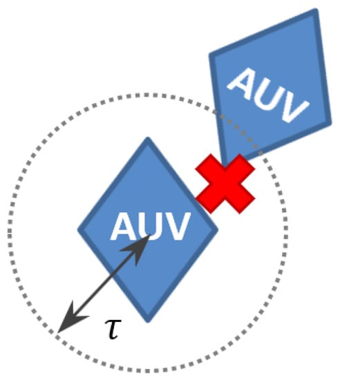 Figure 6. AUVs collision detection.
 - Task completion reward is determined by whether the AUVs salvage the targets. If AUVs salvage a target at time t, all the AUVs will get the reward, which is also related to the emergency of the target. The reward for the task completion is defined as
Then, the reward obtained by in a time step can be calculated as
5. Automatic Policy Amendment Algorithm (APAA)
APAA we proposed is to get the task sequence of each AUV when they finish the entire TA. AUVs will add the task sequence into their Task Sequence Matrix (TSM), if they get a high TCR in a TA. TCR is taken as the AUVs’ reference to each task sequence when making policy decision in the future. Entropy is used to measure the uncertainty for TSM to ensure the diversity of AUVs’ learning samples. SR enable AUVs to balance TCR with their own reward. The amendment probability associated with TSM is generated to affect the AUVs’ action probability distribution, to improve the sample quality, and to accelerate DDQN training.
5.1. Task Sequence Matrix (TSM)
The task sequence represents the order in which salvages the targets in each task allocation. In general, the higher the team cumulative reward (TCR) of a task sequence in an environment, the more valuable it is. Let the amount of the records in TSM be N. Each AUV preserves a matrix to store its own task sequence. Meanwhile, is used to represent the TCR corresponding to the row i in TSM. When a new task sequence emerges, each AUV updates it to TSM by removing the sequence with the lowest TCR if it meets
where is the cumulative reward obtained by during TA.
Table 1 shows the top 10 optimal task sequences generated by the three AUVs after fifty iterations. For each in the table, the corresponding column j indicates the jth target performs, and the jth target that executes is denoted as . For example, and appear the most frequently in , indicating that can contributes a higher TCR if it performs or in .

Table 1.
10 optimal task sequences in the TSMs.
5.2. Automatic Policy Amendment Matrix (APAM)
In a TA, the target selection preference of the AUVs will determine the task completion efficiency, as described in Table 1. We wish to use TSM to influence the preference the AUVs have to perform the task. As a result, a matrix called APAM is constructed by evaluate TSM through three indicators including TCR, entropy and SR. It is worth noting that represents the probability that AUVs selects when performing , where represents the jth target performed by an AUV.
- (1)
- Team Cumulative Reward (TCR)
The TCR is designed to assign the importance to each sequence in TSM with different weights. The higher TCR of the sequence, the greater the influence on the AUVs. The weight of each sequence in TSM is defined as
where and are the lowest and highest TCR the AUVs can achieve, respectively.
Then, for each , the weight corresponding to the AUVs selecting target in performing is calculated according to as
where is a matrix.
Finally, Equation (22) is used to transform into probability matrix .
- (2)
- Entropy
Based on the update mode of TSM mentioned in Section 5.1, we know that TSM will record a new sequence with a TCR greater than the worst sequence in TSM. From Table 1, may select , , and , when performing . However, with the TSM updated by new sequences, the diversity of the targets in TSM may decrease dramatically, and may only select after several iterations. This is not expected in early training, because it will converge to a non-optimal policy. The entropy is used to measure the effect of sequences in TSM on the diversity of AUVs behaviors, and based on entropy, multiple similar records with high reward will get lower weights. The entropy weight of a new sequence is calculated by multiplying the change in TSM’s average TCR by the change in TSM’s entropy after it is added to TSM.
For the column k in TSM, the number of occurrences of is updated as
where C is a matrix and is transformed into probability matrix in the same way as Equation (22). After that, is calculated by
When a new sequence is added, the entropy of TSM is affected. For each sequence in TSM, the weight under the entropy metric is
where and are the average TCR of TSM before and after the new sequence is added, respectively. and are the entropy before and after a new sequence is added, respectively.
Similar to Equation (21), the weights of each target performed by AUVs in different order according to can be calculated as
Note that we transform into probability matrix in the same way as Equation (22).
- (3)
- Subtask Reward (SR)
SR is defined as the cumulative reward obtained by an AUV during the salvage of ith target, aiming to make the AUV balance the TCR and its own reward based on the actual environment. Let be a matrix, representing the cumulative reward for finishing . Based on TSM, the weight of each sequence is calculated as
Then, we have
Finally, the probability matrix is calculated for the by Equation (22).
- (4)
- Probability Weighted
, and are the probability matrices that each target selected by AUVs according to three different indicators under different orders, respectively. In addition, if the variance of a subtask reward in TSM is large, the selected target is considered to has a great influence on the TCR. In this case, will have a high proportion coefficient, calculated as
where represents the column j of , is the smaller of two values, is the variance of the data set, and is used to restrict the influence of . The trade-off between reward and entropy in TSM records has the same coefficient. The APAM is given by
- (5)
- Probability Prediction
APAM is updated through the new sequences, and the probability changes in the historical experience of the matrix can be used as the momentum to predict the future change of APAM, and can furtherly accelerate DDQN training. The momentum matrix is constructed as
where is the change in the momentum of APAM. , and . is updated by the proportional coefficient when the new sequence satisfies the update conditions of TSM, otherwise, the attenuation of is carried out according to a certain coefficient. The prediction of the new APAM is given as
5.3. Action Conduct by APAM
As shown in Table 2, the APAM is generated by the TSM. Obviously, different AUVs have different preferences for the targets. This preference is applied to reduce the state action space and solve the undirected problem of exploration in traditional RL. Q value is converted into probability by softmax, and then according to the information provided by the APAM, the probability is amended. A proper amend method will lead to a good effect of training. The action distribution is the trade-off in the current environment with multiple constraints, while the probability generated by APAM only represents which target has a higher priority for execution. The probability of an action will be motivated or restrained according to the distribution of action instead of the distribution of APAM. If AUVs’ estimation of an action is similar to the expected behavior in APAM, the action will be motivated according to the similarity between the action and the expected direction of APAM, otherwise, it will not be motivated. In fact, motivating one action means inhibiting others, so it is no need to perform additional inhibiting operations for other actions.
Table 2.
The APAM of the three AUVs.
When performs , the column j in the APAM will influence its decision. Let represent the probability that moves in each direction. For each in , the positional relationship between each unfinished target and is calculated, then calculating the cosine similarity between these positional relationships and , and finally amending according to the APAM of
where represents the cosine similarity of two vectors.
5.4. Algorithm Summarize
The Algorithm 1 gives the algorithm flow for APAA.
| Algorithm 1 APAA. |
| Input: Nu, Nm, D, EPISODE, L, M. Output: . 1: Initialize: , , , , , . 2: for to do 3: ; 4: Generate APAM by Equations (20)–(30); 5: while is not terminal state do 6: for to do 7: Generate action probability distribution according to state ; 8: if then 9: if then 10: ; 11: end if 12: for to D do 13: is corrected according to Equation (33); 14: end for 15: end if 16: Choose action by -greedy according to , and get reward ; 17: Put into ; 18: end for 19: ; 20: end while 21: For a new sequence, update TSM according to Equation (19); 22: if then 23: A batch samples randomly selected from ; 24: Training network by Equation (13); 25: end if 26: Executed after several iterations; 27: end for |
6. Simulation Results
In this section, some simulation results for APAA are presented and compare them with those obtained by DDQN, Priority Experience Replay (PER) and Proximal Policy Optimization Clip (PPO-Clip). The simulation is implemented using MATLAB 2018b, and the personal computer is configured with Intel(R) Core(TM) i7-10700 CPU @2.90GHz, 8GigaBytes (GB) RAM.
6.1. Experiment Parameters
The experiment we designed involves a group of three AUVs and five targets distributed in the 10 m × 10 m ocean current region, and the ocean current is modeled by Equation (1). The weight of some targets is greater than the power of AUVs, so they need to be salvaged by the cooperation of multiple AUVs. In the experimental comparison, each algorithm has the same network parameters and structure, and the same initial conditions. Table 3 shows the network and training parameters.
Table 3.
Network structure and training parameters.
-greedy exploration strategy is adopted in action selection. At each step, AUVs randomly select an action with a probability , and with a probability 1- select the action with the highest expected reward. In addition, the decay factor is used to cause to decrease with iterations to increase the probability of choosing the optimal action. is updated after the each training of policy as
Parameters of the RL are shown in Table 4.
Table 4.
Parameters of the RL training.
Table 5 shows the parameters used in APAA. The values of these parameters affect the performance of APAA. First of all, the effect of APAA actually depends on the experience in TSM. N with small value will lead to insufficient experience diversity in TSM and trap into non-optimal policy easily. Then, although let the AUVs have the ability to balance between the team and itself, its value should not be large in collaborative task, as this may cause the task to fail. Finally, and control changes, but both should have a large value because TSM experience collection is essentially Monte Carlo sampling, and noise from random sampling can cause instability.
Table 5.
Parameters of APAA algorithm.
Table 6 and Table 7 show the attributes of the AUVs and the targets, respectively. In the experiment, the initial positions of the AUVs and the targets are randomly initialized within the ocean current region, the weights of the targets are randomly initialized between 2kg and 5kg, the powers of the AUVs are randomly initialized between 1 kg and 4 kg, and AUVs’ velocity are randomly initialized between 1 m/s and 3 m/s. For convenience, we show a set of parameters.
Table 6.
Attributes of the AUVs.
Table 7.
Attributes of the targets.
Parameters involved in the TA model are shown in Table 8.
Table 8.
Parameters of the TA.
6.2. Experiment Result
We compare APAA with DDQN, PER and PPO-Clip in the same scenario and run them several times to get average performance. The performance is shown in Figure 7, and APAA achieves the best convergence performance compared with the other algorithms under the same episode. In fact, the task in this paper is a typical of multi-objective optimization problem, which generally results in a large state-action space. It is clear that DDQN requires a lot of exploration to converge in the complex task and has weak stability in convergence. PER based on DDQN takes advantage of the TD-error of the samples to carry out priority sampling, which improves the sample efficiency. The advantage of PER became visible after the first 2000 iterations and achieves better performance than DDQN. PPO-Clip is an off-policy algorithm based on Actor-Critic, which improves the intelligence of AUVs in an adversative way and achieves the weakest performance. In addition, the convergence time of the algorithms is given in Table 9, and APAA has the highest efficiency. By contrast, PPO-Clip is hard to have a high efficiency due to training for two networks. PER uses the sum tree to improve the sampling efficiency, but still has a high time cost in updating the priority of the samples and sampling.
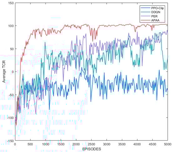
Figure 7.
Team cumulative reward (TCR) of the team.
Table 9.
Convergence time of the algorithms.
From Section 4.3, TCR consists of four goals. The performance of task completion reward is shown in Figure 8. In the experiment, the maximum reward for salvaging the five targets is 125. APAA gets the highest task completion reward compared with the other algorithms.
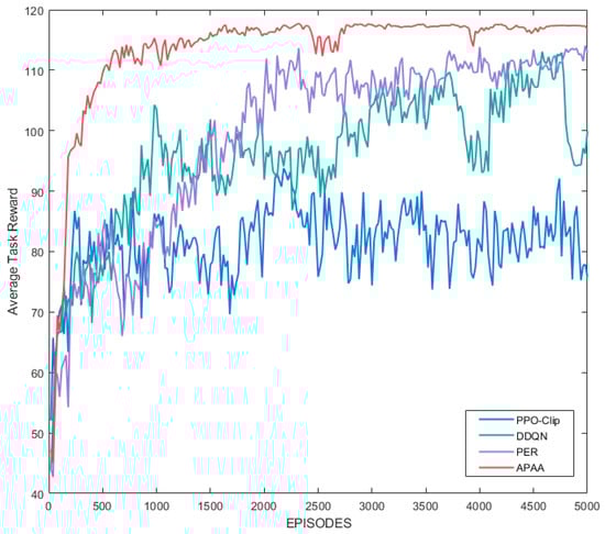
Figure 8.
Task reward of the team.
Figure 9 shows the performance of the algorithms in energy loss and collision detection, respectively. In Table 6, the total energy reserve carried by AUVs is 1800 J, and APAA only consumes 7% of the energy to salvage all the targets, that is, it can plan a better path in the ocean current. In addition, the performance of APAA in collision detection also highlights the lower probability of collisions occurring during AUVs executing the task.
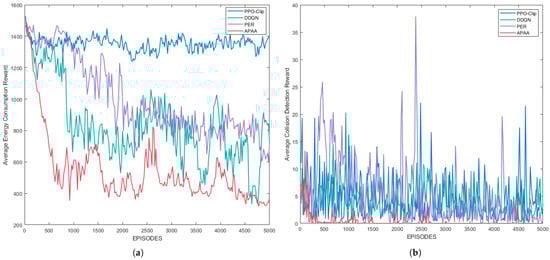
Figure 9.
The performance of (a) energy consumption and (b) collision detection.
Table 10 shows the performance of the algorithms after convergence. A performance is provided, time consuming, indicating the time cost the AUVs take to complete the task.
Table 10.
Convergence performance of the algorithms (After 5000 episodes).
Figure 10 shows the trajectories of the AUVs and targets with APAA after training. The hexagonal stars are the starting positions of the AUVs, and the asterisks are the end positions of the AUVs. The squares are the starting positions of the targets, the circles are the positions when the targets are salvaged, and the arrows are the direction of the ocean current at the coordinates. As can be seen from the path planned by the AUVs at each step, they always take full advantage of the ocean current moving in the same direction.
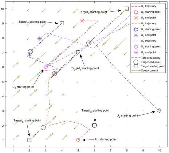
Figure 10.
The trajectories of the AUVs and the targets in APAA.
7. Analysis
In this section, the validity and computational complexity of APAA theoretically are presented.
7.1. Validity Analysis
In order to speed up RL, the policy subspace with greater potential benefits in the state-action space needs to be consider. Let be the policy in the kth iteration, and be the probability of choosing an action from the state-action space. According to APAA, we have
where is the probability amendment for the state-action pair.
If is a better state-action pair, , otherwise, . As a result, and , for and , we have . The subspace will not be explored when , so APAA is more efficient than DDQN with the same episodes.
7.2. Computational Complexity Analysis
The computational cost of APAA mainly consists of two parts: calculating APAM by TSM and amending AUVs’ decision by APAM. First, let the number of actions of the AUVs be d, TSM be an matrix, and . In Section 5.2, each element in TSM is evaluated by TCR, SR, and Entropy to generate APAM. Thus, the computational complexity of this part can easily be estimated as . After that, APAM amends the probability distribution for the actions of the AUVs, and the computational complexity of this part can be expressed as . Finally, the computational cost of APAA is the sum of the computational complexity of the two parts, i.e., .
Although APAA has a high computational complexity in form, amending the action distribution with the drifting targets that have been salvaged are not considered. As a result, the computational complexity of the second part would decrease with the progress of the overall task, so that it can almost be ignored. In addition, the samples of RL are only related to the actions of the AUVs at each time step, and it is difficult for AUVs to extract the relationship between behaviors and task results from the massive samples. However, APAM extracts information related to the task, which can effectively accelerate the learning speed, so as to believe that such a computational cost is worth it. In contrast, the computational complexity of PER is related to the size of the replay buffer, and the computational complexity of PER increases dramatically for complex tasks. The parameter sensitivity of PPO-Clip and the need to train two networks result in higher computational complexity. Therefore, APAA also outperforms PER and PPO-Clip at the same training time.
8. Conclusions
In this paper, a new RL approach is proposed to solve the task allocation problem of multi-AUV in ocean currents. First, the ocean current and a reward function are constructed. The ocean current, the energy, the task emergency and the collision with other AUVs need to be taken into account when AUVs perform the task. Many classical RL algorithms improve the efficiency of traditional samples, but a problem is that traditional samples are not directly related to the task, which makes it difficult for AUVs to understand how their behavior affects the final result. To overcome this drawback, the Automatic Policy Amendment Algorithm (APAA) is introduced. TSM is generated by the task sequences for each AUV, which represents the task preference for AUVs to obtain the highest TCR. Such information related to the task can effectively guide the policy learning. After that, APAM is calculated by TSM, and uses TCR, entropy and SR to adjust the decision of AUVs. Finally, the simulation results show that APAA accelerates the convergence and improves the overall performance compared with the DDQN, PER and PPO-Clip. In future work, we will deal with more complex optimal planning tasks in 3D scenarios.
Author Contributions
Conceptualization, Z.Z. and C.D.; methodology, C.D. and Z.Z.; software, C.D.; validation, C.D.; writing original draft preparation, C.D.; writing review and editing, C.D. and Z.Z. All authors have read and agreed to the published version of the manuscript.
Funding
The authors are grateful for the National Natural Science Foundation of China (No. 61873033), the Science Foundation of Fujian Normal University (No. Z0210553), and the Natural Science Foundation of Fujian Province (No. 2020H0012, No. 2017J01740).
Institutional Review Board Statement
Not applicable.
Informed Consent Statement
Not applicable.
Data Availability Statement
Not applicable.
Conflicts of Interest
The authors declare no conflict of interest.
References
- Allotta, B.; Bartolini, F.; Caiti, A.; Costanzi, R.; Di Corato, F.; Fenucci, D.; Gelli, J.; Guerrini, P.; Monni, N.; Munafò, A.; et al. Typhoon at CommsNet13: Experimental Experience on AUV Navigation and Localization. Annu. Rev. Control 2015, 40, 157–171. [Google Scholar] [CrossRef]
- Allotta, B.; Costanzi, R.; Pugi, L.; Ridolfi, A. Identification of the Main Hydrodynamic Parameters of Typhoon AUV from A Reduced Experimental Dataset. Ocean. Eng. 2018, 147, 77–88. [Google Scholar] [CrossRef]
- Liu, Q.; Sun, B.; Zhu, D. A Multi-AUVs Cooperative Hunting Algorithm for Environment with Ocean Current. In Proceedings of the 2018 37th Chinese Control Conference, Wuhan, China, 25–27 July 2018. [Google Scholar]
- Li, L.; Li, Y.; Zeng, J.; Xu, G.; Zhang, Y.; Feng, X. A Research of Multiple Autonomous Underwater Vehicles Cooperative Target Hunting Based on Formation Control. In Proceedings of the 2021 6th International Conference on Automation, Control and Robotics Engineering, Dalian, China, 15–17 July 2021. [Google Scholar]
- Wu, J.; Song, C.; Ma, J.; Wu, J.; Han, G. Reinforcement Learning and Particle Swarm Optimization Supporting Real-Time Rescue Assignments for Multiple Autonomous Underwater Vehicles. IEEE Trans. Intell. Transp. Syst. 2021. accepted. [Google Scholar] [CrossRef]
- Zhu, Z.; Wu, Z.; Deng, Z.; Qin, H.; Wang, X. An Ocean Bottom Flying Node AUV for Seismic Observations. In Proceedings of the 2018 IEEE/OES Autonomous Underwater Vehicle Workshop (AUV), Porto, Portugal, 6–9 November 2018. [Google Scholar]
- Liu, S.; Xu, H.L.; Lin, Y.; Gao, L. Visual Navigation for Recovering an AUV by Another AUV in Shallow Water. Sensors 2019, 19, 1889. [Google Scholar] [CrossRef] [PubMed] [Green Version]
- Shen, C.; Buckham, B.; Shi, Y. Modified C/GMRES Algorithm for Fast Nonlinear Model Predictive Tracking Control of AUVs. IEEE Trans. Control Syst. Technol. 2017, 25, 1896–1904. [Google Scholar] [CrossRef]
- Carreras, M.; Hernandez, J.D.; Vidal, E.; Palomeras, N.; Ribas, D.; Ridao, P. Sparus II AUV-A Hovering Vehicle for Seabed Inspection. IEEE J. Ocean. Eng. 2018, 43, 344–355. [Google Scholar] [CrossRef]
- Kojima, M.; Asada, A.; Mizuno, K.; Nagahashi, K.; Katase, F.; Saito, Y.; Ura, T. AUV IRSAS for Submarine Hydrothermal Deposits Exploration. In Proceedings of the 2016 IEEE/OES Autonomous Underwater Vehicles (AUV), Tokyo, Japan, 6–9 November 2016. [Google Scholar]
- Savkin, A.V.; Verma, S.C.; Anstee, S. Optimal Navigation of an Unmanned Surface Vehicle and an Autonomous Underwater Vehicle Collaborating for Reliable Acoustic Communication with Collision Avoidance. Drones 2022, 6, 27. [Google Scholar] [CrossRef]
- Yu, X.; Gao, X.; Wang, L.; Wang, X.; Ding, Y.; Lu, C.; Zhang, S. Cooperative Multi-UAV Task Assignment in Cross-Regional Joint Operations Considering Ammunition Inventory. Drones 2022, 6, 77. [Google Scholar] [CrossRef]
- Ferri, G.; Munafo, A.; Tesei, A.; LePage, K. A Market-based Task Allocation Framework for Autonomous Underwater Surveillance Networks. In Proceedings of the Oceans Aberdeen Conference, Aberdeen, UK, 19–22 June 2018. [Google Scholar]
- Ma, Y.N.; Gong, Y.J.; Xiao, C.F.; Gao, Y.; Zhang, J. Path Planning for Autonomous Underwater Vehicles: An Ant Colony Algorithm Incorporating Alarm Pheromone. IEEE Trans. Veh. Technol. 2019, 68, 141–154. [Google Scholar] [CrossRef]
- Han, G.; Gong, A.; Wang, H.; Martinez-Garcia, M.; Peng, Y. Multi-AUV Collaborative Data Collection Algorithm Based on Q-learning in Underwater Acoustic Sensor Networks. IEEE Trans. Veh. Technol. 2021, 70, 9294–9305. [Google Scholar] [CrossRef]
- Xi, L.; Zhou, L.; Xu, Y.; Chen, X. A Multi-Step Unified Reinforcement Learning Method for Automatic Generation Control in Multi-area Interconnected Power Grid. IEEE Trans. Sustain. Energy 2020, 12, 1406–1415. [Google Scholar] [CrossRef]
- Zhang, J.; Yang, Q.; Shi, G.; Lu, Y.; Wu, Y. UAV Cooperative Air Combat Maneuver Decision Based on Multi-agent Reinforcement Learning. J. Syst. Eng. Electron. 2021, 32, 1421–1438. [Google Scholar]
- Zhang, Z.; Wang, D.; Gao, J. Learning Automata-based Multiagent Reinforcement Learning for Optimization of Cooperative Tasks. IEEE Trans. Neural. Netw. Learn. Syst. 2021, 32, 4639–4652. [Google Scholar] [CrossRef] [PubMed]
- Guo, W.; Tian, W.; Ye, Y.; Xu, L.; Wu, K. Cloud Resource Scheduling with Deep Reinforcement Learning and Imitation Learning. IEEE Internet Things J. 2021, 8, 3576–3586. [Google Scholar] [CrossRef]
- Hoseini, S.A.; Hassan, J.; Bokani, A.; Kanhere, S.S. In Situ MIMO-WPT Recharging of UAVs Using Intelligent Flying Energy Sources. Drones 2021, 5, 89. [Google Scholar] [CrossRef]
- Sutton, R.; Barto, A. Reinforcement Learning:An Introduction. IEEE Trans. Neural Netw. 1998, 9, 1054. [Google Scholar] [CrossRef]
- Watkins, C.; Dayan, P. Q-learning. Mach. Learn. 1992, 8, 279–292. [Google Scholar] [CrossRef]
- Geist, M.; Pietquin, O. Algorithmic Survey of Parametric Value Function Approximation. IEEE Trans. Neural Netw. Learn. Syst. 2013, 24, 845–867. [Google Scholar] [CrossRef] [Green Version]
- Mnih, V.; Kavukcuoglu, K.; Silver, D.; Rusu, A.A.; Veness, J.; Bellemare, M.G.; Graves, A.; Riedmiller, M.; Fidjeland, A.K.; Ostrovski, G. Human-level Control through Deep Reinforcement Learning. Nature 2015, 518, 529–533. [Google Scholar] [CrossRef]
- Van Hasselt, H.; Guez, A.; Silver, D. Deep Reinforcement Learning with Double Q-learning. In Proceedings of the 30th Association for the Advancement of Artificial Intelligence (AAAI) Conference on Artificial Intelligence, Phoenix, AZ, USA, 12–17 February 2016. [Google Scholar]
- Lin, L.J. Self-Improving Reactive Agents Based on Reinforcement Learning, Planning and Teaching. Mach. Learn. 1992, 8, 293–321. [Google Scholar] [CrossRef]
- Schaul, T.; Quan, J.; Antonoglou, I.; Silver, D. Prioritized Experience Replay. In Proceedings of the International Conference on Learning Representations 2016, San Juan, Puerto Rico, 2–4 May 2016. [Google Scholar]
- Horgan, D.; Quan, J.; Budden, D.; Barth Maron, G.; Hessel, M.; Van Hasselt, H.; Silver, D. Distributed Prioritized Experience Replay. In Proceedings of the International Conference on Learning Representations (ICLR), Vancouver, BC, Canada, 30 April–3 May 2018. [Google Scholar]
- Zhao, Y.; Liu, P.; Zhao, W.; Tang, X. Twice Sampling Method in Deep Q-network. Acta Autom. Sin. 2019, 14, 1870–1882. [Google Scholar]
- Zhang, H.J.; Qu, C.; Zhang, J.D.; Li, J. Self-Adaptive Priority Correction for Prioritized Experience Replay. Appl. Sci. 2020, 10, 6925. [Google Scholar] [CrossRef]
- Ramicic, M.; Bonarini, A. Entropy-based Prioritized Sampling in Deep Q-learning. In Proceedings of the 2017 2nd International Conference on Image, Vision and Computing (ICIVC), Chengdu, China, 2–4 June 2017. [Google Scholar]
- Yang, D.; Qin, X.; Xu, X.; Li, C.; Wei, G. Sample-efficient Deep Reinforcement Learning with Directed Associative Graph. China Commun. 2021, 18, 100–113. [Google Scholar] [CrossRef]
- Pathak, D.; Agrawal, P.; Efros, A.A.; Darrell, T. Curiosity-driven Exploration by Self-supervised Prediction. In Proceedings of the 30th IEEE/CVF Conference on Computer Vision and Pattern Recognition Workshops (CVPRW), Honolulu, HI, USA, 21–26 July 2017. [Google Scholar]
- Zhu, J.; Wei, Y.T. Adaptive Deep Reinforcement Learning for Non-stationary Environments. Sci. China Inf. Sci. 2021. accepted. [Google Scholar]
- Kumra, S.; Joshi, S.; Sahin, F. Learning Robotic Manipulation Tasks via Task Progress Based Gaussian Reward and Loss Adjusted Exploration. IEEE Robot. Autom. Lett. 2022, 7, 534–541. [Google Scholar] [CrossRef]
- Shi, H.; Xu, M. A Multiple-Attribute Decision-Making Approach to Reinforcement Learning. IEEE Trans. Cogn. Dev. Syst. 2020, 12, 695–708. [Google Scholar] [CrossRef]
- Pakizeh, E.; Palhang, M.; Pedram, M.M. Multi-criteria Expertness Based Cooperative Q-learning. Appl. Intell. 2013, 39, 28–40. [Google Scholar] [CrossRef]
- Yao, X.; Wang, F.; Wang, J. Energy-optimal Path Planning for AUV with Time-variable Ocean Currents. Control Decis. 2020, 35, 2424–2432. [Google Scholar]
Publisher’s Note: MDPI stays neutral with regard to jurisdictional claims in published maps and institutional affiliations. |
© 2022 by the authors. Licensee MDPI, Basel, Switzerland. This article is an open access article distributed under the terms and conditions of the Creative Commons Attribution (CC BY) license (https://creativecommons.org/licenses/by/4.0/).