Quantification of Grassland Biomass and Nitrogen Content through UAV Hyperspectral Imagery—Active Sample Selection for Model Transfer

Abstract

Accurate retrieval of grassland traits is important to support management of pasture production and phenotyping studies. In general, conventional methods used to measure forage yield and quality rely on costly destructive sampling and laboratory analysis, which is often not viable in practical applications. Optical imaging systems carried as payload in Unmanned Aerial Vehicles (UAVs) platforms have increasingly been proposed as alternative non-destructive solutions for crop characterization and monitoring. The vegetation spectral response in the visible and near-infrared wavelengths provides information on many aspects of its composition and structure. Combining spectral measurements and multivariate modelling approaches it is possible to represent the often complex relationship between canopy reflectance and specific plant traits. However, empirical models are limited and strictly represent characteristics of the observations used during model training, therefore having low generalization potential. A method to mitigate this issue consists of adding informative samples from the target domain (i.e., new observations) to the training dataset. This approach searches for a compromise between representing the variability in new data and selecting only a minimal number of additional samples for calibration transfer. In this study, a method to actively choose new training samples based on their spectral diversity and prediction uncertainty was implemented and tested using a multi-annual dataset. Accurate predictions were obtained using hyperspectral imagery and linear multivariate models (Partial Least Squares Regression—PLSR) for grassland dry matter (DM; $R^2$ = 0.92, $RMSE$ = 3.25 dt ha${}^{-1}$), nitrogen (N) content in % of DM ($R^2$ = 0.58, $RMSE$ = 0.27%) and N-uptake ($R^2$ = 0.91, $RMSE$ = 6.50 kg ha${}^{-1}$). In addition, the number of samples from the target dates added to the training dataset could be reduced by up to 77% and 74% for DM and N-related traits, respectively, after model transfer. Despite this reduction, $RMSE$ values for optimal transfer sets (identified after validation and used as benchmark) were only 20–30% lower than those values obtained after model transfer based on prediction uncertainty reduction, indicating that loss of accuracy was relatively small. These results demonstrate that considerably simple approaches based on UAV hyperspectral data can be applied in preliminary grassland monitoring frameworks, even with limited datasets.

1. Introduction

Adequate grassland management is required to ensure sustainable and rentable cattle production, especially taking into account the potentially high environmental impacts of this activity. The management of pasture areas is complex, in particular for intensive production systems with multiple mowing and/or grazing events over the growing season. For farmers, determining the quantity and quality of forage available in-situ is essential since it is the least expensive source of feed and optimizing the utilization of this resource is crucial to reduce production costs [1]. In this sense, choosing the right time for harvesting or grazing a given field is important and involves a trade-off between yield and biomass nutritional value, since dry matter accumulation over time is generally followed by reduction in nutritional quality, in particular regarding digestibility [2].

Exploring the full productive potential of pasture fields requires sound fertilization planning. Considering the high amount of biomass extracted and the relatively low nutrient use efficiency, depending on the management practices related to nitrogen for example [3], it is important to have accurate estimates of yield and nutrient uptake to assist farmers in the decision-making process related to fertilizer and amendment application. Current approaches used to evaluate yield or sward height involve visual assessment, rising-plate meters or electronic probes since destructive samples are labour demanding and expensive, therefore inadequate for practical use. In addition, grass quality parameters are not often monitored since their assessment depends on laboratory analysis, which increases the costs and complexity of the evaluation methods conventionally used. As an alternative, remote sensing techniques have been proposed in the literature as viable tools to assess quantity and quality of grassland production.

In recent years, particular attention has been given to Unmanned Aerial Vehicles (UAVs) as affordable and flexible platforms for agricultural studies and applications. Different sensors can be carried as payload by UAVs, allowing a comprehensive characterization of the vegetation. However, optical sensors, from high resolution RGB to multispectral and hyperspectral cameras, are generally the most accessible and informative sensing solutions available for general crop assessment and growth monitoring [4,5]. The spectral response of the plant canopy in the visible and near-infrared (NIR) regions (i.e., wavelengths between 450 and 900 nm) is strongly correlated to several biophysical and biochemical characteristics such as biomass and chlorophyll or nitrogen content [5,6]. At the same time, UAV-based imaging systems provide spatially continuous information, which is potentially advantageous when compared to point-based measurements regarding the description of spatial patterns and subsequent adjustment of management operations.

The use of UAV-based optical imaging systems for the characterization of forage traits has increasingly been explored in the literature, specially concerning yield estimation [7,8,9]. Retrieval of pasture quality parameters such as crude protein content have been less frequently studied, but research interest in this topic is also increasing due to its importance to the planning of animal feeding and fertilizer application [10]. However, most of the studies investigating the use of UAVs for forage assessment and management focus on single harvests or growing seasons [11], limiting their conclusions to specific cases or small datasets. As other plants, grasses are subject to intra- and inter-annual growth variability caused by different factors such as temperature, water availability or changes in management practices. In addition, pastures are perennial and monitoring systems need to cope with considerable variation in measuring conditions since frequent data acquisition is generally required for relatively extensive periods of time to allow informed decisions. Therefore, prediction models for grassland traits based on limited or small spectral datasets will be prone to errors and large uncertainties when applied to samples acquired on other years or under different measurement conditions than those already described by observations available for model training.

Approaches used to estimate vegetation traits based on canopy spectral measurements in the optical domain can be roughly divided in empirical and physically-based methods [5,12]. While the first case relies on a training dataset to fit prediction models the later requires, in general, adequate parametrization of a Radiative Transfer Model (RTM) to translate spectral information into vegetation characteristics. RTM-based frameworks have greater generalization potential but performance might eventually be suboptimal, in particular for complex systems composed of multiple cultivars and/or crop mixtures, which makes parametrization more difficult. In turn, empirical models adapt well to complex datasets however their application is restricted to observations sharing the characteristics of the training data. Considering that fast evaluation and deployment of monitoring solutions based on UAV optical imagery is desirable, empirical models can be an initial option, especially for complex systems not yet well characterized or fully described.

Extending pre-existing training datasets to better represent new observations can reduce costs associated to monitoring frameworks that rely on empirical models to assist in general crop management. The purposeful or active selection of additional calibration samples offers an alternative to take advantage of data already available while improving model performance for newly acquired measurements [13]. Different criteria can be considered to choose samples from a pool of available unlabelled cases for model training, and some of the most relevant aspects for this selection are sample diversity (i.e., how much the selected samples in the target dataset scatters across the feature space) and prediction uncertainty (i.e., how unsure the current modelling framework is about predictions for individual samples in the target domain) [14,15,16]. One way to broadly divide active learning approaches is to consider if they are supervised or unsupervised [15,17,18,19,20]. While unsupervised algorithms do not rely on labelled examples to further select candidate datasets for annotation and model fitting, supervised methods need at least an initial set of reference samples and usually also require an initial predictive model. Unsupervised approaches are attractive due to their flexibility and relatively straightforward implementation, however they are not optimal. Conversely, supervised methods are at least weakly optimal, through a heuristic approximation, and generally lead to better performance [20].

In this context, the objectives of this study are: (i) evaluate the use of UAV hyperspectral imagery for the quantification of forage yield (dry matter in dt ha${}^{-1}$) and nitrogen nutrition status (nitrogen content in % of dry matter and nitrogen uptake in kg ha${}^{-1}$); (ii) extend the research presented by Capolupo et al. [10] to a multi-annual assessment of grassland traits retrieval, closer to real application scenarios; and (iii) implement and validate a supervised approach for model transfer, searching to add informative samples from the target date to a pre-existing source dataset, based on sample diversity and prediction uncertainty within an adapted Active Learning framework [17]. The main focus is to demonstrate that even considerably simple approaches applied to small datasets can result in relatively accurate predictions of grassland traits, indicating their spatial patterns and providing initial site-specific information to assist farmers in pasture management.

2. Material and Methods

2.1. Study Site and Experimental Design

The data used in this study was acquired in an experimental site in Germany, located near the city of Kleve (51${}^{\circ }$47${}^{\prime }$12.5${}^{″}$ N, 6${}^{\circ }$10${}^{\prime }$08.7${}^{″}$ E; as also described by Capolupo et al. [10]). In this site, 60 plots measuring 1.5 by 8.0 m were arranged in four blocks and cultivated with ryegrass (Lolium perenne) from 2012 to 2019 (Figure 1). In each block, 15 different nitrogen (N) treatments were randomly applied to the experimental plots with four repetitions (i.e., one treatment per plot and one repetition per block). The treatments comprised different rates of inorganic (five levels of Calcium Ammonium Nitrate—CAN: 0, 85, 115, 170, 230, and 340 kg of N ha${}^{-1}$) and organic fertilizer (three levels of slurry: 170, 230 and 340 kg of N ha${}^{-1}$). For the treatments involving organic fertilizer, one additional factor considered was the number of consecutive years (from one to three years) in which these treatments were applied. The experiment was designed to represent the most common scenarios of N management adopted by farmers in the study region (i.e., 170 kg of N ha${}^{-1}$, maximum normally allowed by law) and deviations from that (e.g., 230 kg of N ha${}^{-1}$, maximum allowed in ‘non-grazing’ regime; and 340 kg N ha${}^{-1}$, estimate maximum possible uptake) allowing an evaluation of the grassland response to different N fertilization planning and sources.

2.2. Measurement of above Ground Biomass and Nitrogen Content

Grassland traits were periodically evaluated since the start of the experiment in 2012. At the plot level, dry above-ground biomass was measured by harvesting and drying fresh vegetative material (for 24 h at 105 ${}^{\circ }$C). Further analysis of the collected material at treatment level (i.e., composite sample representing all plots of a given treatment) for each harvest date was carried out by the Agriculture Research Institute North Rhine-Westphalia in Germany (Landwirtschaftliche Untersuchungs- und Forschungsanstalt Nordrhein-Westfalen—LUFA NRW) following methods of the German Association of Agricultural Research and Research Institutes (Verband der Landwirtschaftlichen Untersuchungs- und Forschungsanstalten—VDLUFA). For each sample, multiple properties were determined (i.e., crude ash, crude fiber, sodium and potassium contents) however we focus here on nitrogen (N) content, which was expressed in (i) percentage of dry matter; and (ii) in kg ha${}^{-1}$, after being multiplied by the average dry matter weight at the treatment level. The final traits evaluated comprised dry matter and N-related properties (N% in dry matter and N-uptake in kg ha${}^{-1}$), since these aspects are of particular interest for the management of nitrogen in intensive grassland systems.

2.3. UAV Hyperspectral and High Resolution Imagery: Acquisition and Pre-Processing

On 2014 and 2017, a total of five UAV flights were performed in the experimental site, always before biomass harvest (DOY 135 and 288 in 2014, and DOY 130, 242 and 299 in 2017). The image acquisition was realized using the WageningenUR Hyperspectral Mapping System (HYMSY), a pushbroom imaging sensor comprising a custom spectrometer (PhotonFocus SM2-D1312 camera—PhotonFocus AG, Lachen, SZ, Switzerland—with a Specim ImSpector V10 2/3 spectrograph—Specim, Spectral Imaging Ltd., Oulu, Finland) and a RGB high resolution photogrammetric camera (Panasonic GX1 16 MP—Panasonic Corp., Osaka, Japan—with 14 mm pancake lens). Further details about the sensor as well as the radiometric and geometric correction of the acquired data can be found in Suomalainen et al. [21].

In general lines, the main steps involved in the hyperspectral data pre-processing were: (i) Digital Numbers (DNs) conversion to radiance units using dark current and flat field calibration; (ii) radiance conversion to reflectance factors based on measurements taken before each flight of a 25% reflectance Spectralon panel; (iii) geometric correction of the hyperspectral datacube through a direct georeferencing procedure, which required external Digital Surface Model (DSM) and Global Navigation Satellite System-Inertial Navigation System (GNSS-INS) data as auxiliary inputs [22]. The DSM in this case was obtained from images taken with the RGB camera, using Structure-from-Motion (SfM) algorithm in the photogrammetric software PhotoScan Pro v1.0.0 (currently Metashape; Agisoft LLC, St. Petersburg, Russia). Adjusted camera orientations that matched the surface model were obtained at the same time the high resolution DSM was derived. These adjusted orientations were used to increase accuracy of the GNSS-INS data before geometric correction of the hyperspectral data. The resulting DSM and updated GNSS-INS data were feed together with the hyperspectral datacube to the PARGE algorithm (v3.2beta, ReSe Applications, Schläpfer and Richter [22]) in order to implement the georeferencing of the hyperspectral images.

The final hyperspectral data used during analysis comprised 101 spectral bands (from 450 up to 950 nm) registered in a 5 nm interval. The Full Width at Half Maximum (FWHM) for the spectral response of each band was approximately 10 nm and the signal measured was smoothed out by resampling the spectra using the same sampling interval but adopting a larger FWHM (30 nm) and assuming a Gaussian spectral response.

An important aspect related to the obtention of the DSMs used in the geometric correction of the hyperspectral data is the parametrization of the dedicated photogrammetric software. For that, image alignment and dense point cloud estimation were implemented using RGB images with full resolution, by setting quality to ‘high’ and ‘ultra-high’ for these steps in the software processing chain, respectively. In addition, camera positioning optimization was performed based on 4 to 8 Ground Control Points (GCPs), depending on the acquisition date, which had their coordinates registered using a Real Time Kinematic (RTK)-GNSS receiver. Also, only focal length, principal point, three radial distortion parameters and two tangential distortion parameters were optimized during processing to avoid overfitting [23]. Before the camera position optimization, sparse point clouds were filtered based on residuals and reconstruction uncertainty (10% of points were removed in each case), as recommended by [24].

Finally, considering a flight height of approximately 30 m, GSD between 0.8 and 1.5 cm was obtained for RGB images while for the hyperspectral data GSD varied between 7.8 and 15.6 cm.

2.4. Prediction of Grassland Traits Based on Hyperspectral Imagery across Different Years

Grassland above ground dry matter (DM, dt ha${}^{-1}$) and nitrogen related traits (N% in DM and N-uptake in kg ha${}^{-1}$) were estimated based on reflectance factors extracted from the UAV hyperspectral imagery. For that, Partial Least Squares Regression (PLSR) was used to represent the relationship between each grassland trait and the canopy spectral response.

In order to match the support of the spectral data and ground truth observations (i.e., area represented by the measurements), the spectral information was averaged at plot level for DM prediction and at the treatment level (comprising generally four plots) for N-related traits. For all cases, analysis was made assuming three scenarios: first using data from each season separately, (i) 2014 or (ii) 2017; and finally (iii) considering both seasons together, which was used as benchmark to evaluate the generalization potential of the models obtained for each season.

The modelling framework adopted in this study was adapted from approaches described by Singh et al. [25] and Wang et al. [26], which include simultaneous estimation of prediction potential and model uncertainty. For that, the complete dataset (comprising 49 observations from each acquisition date for DM, after excluding plots in which the corresponding spectral information acquired was potentially obscured by a metal structure present in the field; or 15 observations from each acquisition date for N-related traits, summarizing information at the treatment level) was randomly split in two parts, 70% used for model calibration and 30% for validation. The calibration set was further divided in two, 2/3 used to fit the prediction models and 1/3 used to test their accuracy. This last sampling procedure was randomly repeated 100 times and the derived models were applied to the test and validation datasets. This procedure allowed not only to estimate the average trait value for each sample but also the associated prediction uncertainty, expressed as standard deviation of prediction.

2.5. Calibration Model Transfer through Active Sample Selection

A calibration set transfer approach was tested as an alternative to increase the portability of prediction models between years, instead of scenario (iii) described in Section 2.4, which would require a relatively large number of samples from the target date (i.e., equal proportion of samples from source and target domains). Estimations made for a given year/season risk to be inaccurate if the model used was trained on a limited number of samples, or if these samples are acquired in a different year/season. This occurs because a small training samples set with limited variability may not adequately represent a new set of observations. Despite that, a pre-existing dataset can potentially contain useful information for estimating properties of new samples, even if source and target domains are not fully comparable. The approach adopted in this study consisted in adding samples from the target domain (i.e., the acquisition date of interest, from a different growing season/year than that of samples initially available for training) to the dataset used to fit the prediction models (i.e., source domain). With this objective, a framework based on Active Learning [16,27] was implemented and evaluated.

The active selection of samples from the target domain to be included in the training dataset was made based on sample diversity and prediction uncertainty. For that, a method well describe by Douak et al. [17] was adapted, which relies on a pool of regressors (abbreviated PAL). These authors have sampled the training dataset in a given number $Sv$ of subsets, down sampling the available observations by a given factor. Considering that the obtained subsets were independent, different models were derived using Kernel Ridge Regression. Therefore it was possible to obtain $Sv$ predictions for each sample from the target domain, and estimate the associated prediction variance for them. Samples with the highest variance were selected for model fitting. It is clear that this approach is very similar to the modelling framework described in Section 2.4, however in our research we have used PLSR and a more conventional bootstrap-based uncertainty estimation.

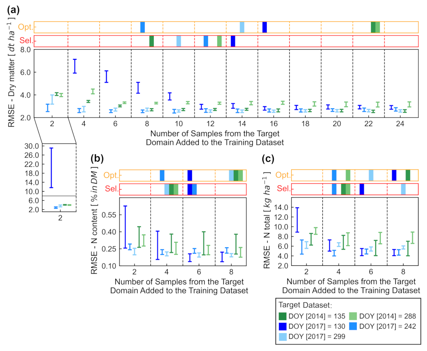
Therefore, our method relied first on prediction models already available, which were derived from the different source datasets; i.e., scenarios (i) and (ii) presented in Section 2.4. With them it was possible to estimate vegetation traits and prediction uncertainty for the target samples, acquired on other years/seasons. In addition, K-means clustering was adopted to group each target dataset according to their spectral variability, using results of Principal Components Analyses (i.e., Principal Components with cumulative explained variance of at least 99.5% in each case) and searching to split the target samples into two clusters. After that, the observation with the largest prediction uncertainty (i.e., standard deviation of prediction) was selected for each cluster. These two samples were added to the training data and a new prediction model was derived. This process was repeated until half of the samples available for a given target date were included in the training dataset. The ‘optimal’ number of samples selected to transfer the prediction model to the target domain was chosen considering all cases in the range of the average uncertainty ±20% of the total uncertainty reduction (i.e., smallest uncertainty value subtracted from the largest one considering the multiple transfer datasets compared for each target date). If there were no cases included in the calculated interval, the number of samples resulting in the highest uncertainty was removed and the average calculated again for the remaining cases, until at least one value was selected. The case closest to the median number of included samples was retained (if multiple cases were in the interval). This criterium was chosen after an empirical evaluation (considering the number of samples used, overall uncertainty reduction achieved for the target data and prediction accuracy for out-of-the bag samples in the calibration dataset), which indicated that selecting samples based on an interval around the average uncertainty resulted in a good compromise between minimizing prediction uncertainty and limiting the number of samples required for model transfer.

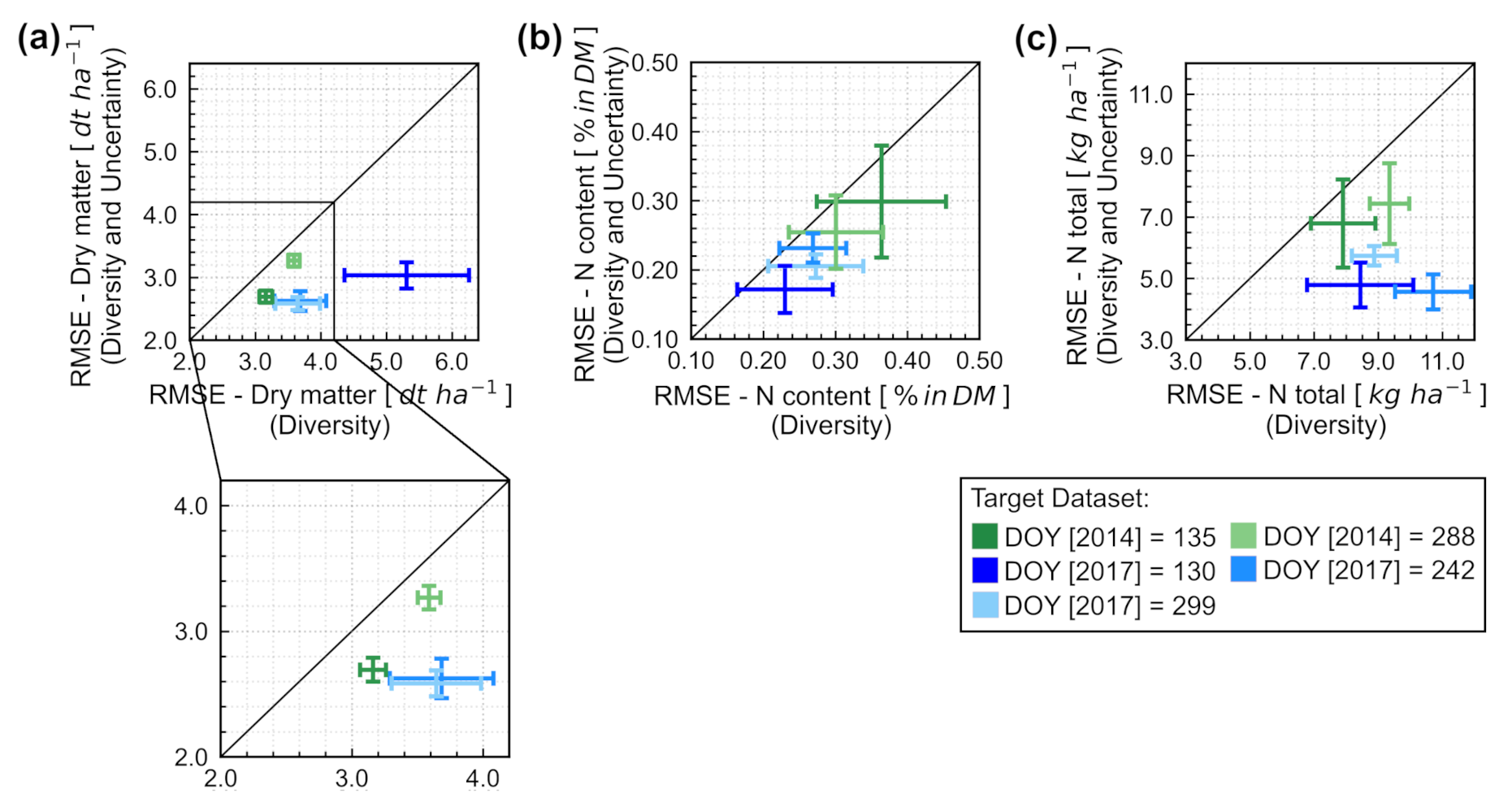
For comparison, the same number of samples identified as ‘optimal’ in each case was selected considering only the spectral information (samples closest to the centroid of each K-means cluster), ignoring the estimated prediction uncertainty. This allowed to assess the added value of taking into account the prediction uncertainty during model transfer. It is also worth mentioning that ground truth reference was assumed to be always available after samples from the target dataset were selected. This is not possible in practice since all samples used during the ‘optimization’ of the training dataset would need to be processed and analysed in laboratory beforehand, therefore with no advantages over scenario (iii) described in Section 2.4. This issue could potentially be circumvented by using predictions of the model available or RTM inversion for a first estimation of traits, for example, resulting in values that could be used to replace ground truth during sample selection. However, for brevity, this aspect was not evaluated in this study since the main objective was to assess whether selecting samples based on prediction uncertainty would be beneficial or not in this context.

2.6. Feature Selection for Grassland Traits Retrieval

The vegetation traits evaluated in this study (i.e., biomass and N-related traits) are linked to the canopy spectral response in ways that can be difficult to distinguish, depending on the spectral region and conditions of data acquisition. Therefore, it is relevant to inspect the importance of the multiple spectral bands or regions for the estimation of each specific grassland trait, so differences and similarities between models can be compared. This analysis can also be used to evaluate the performance of the model transfer approach, allowing one to compare the main variables contributing to the predictions when models are derived from distinct training datasets.

With this objective, Variable Importance in the Projection ($VIP$; [28,29]) was calculated for each model, obtained from the different calibration datasets, and spectral band j, as described by Equations (1) and (2).

$$VI{P}_j=\sqrt{\frac{J\times \left[{\sum }_{f=1}^F{\left(w_{jf}/\parallel w_f\parallel \right)}^2\times SS{Y}_f\right]}{{\sum }_{f=1}^{F}SS{Y}_f}}$$

(1)

$$SS{Y}_f=b_f^2\times t_f^{\prime }\times t_f$$

(2)

where $w_{jf}$ corresponds to the weight of variable j and PLS component f while $SS{Y}_f$ represents the sum of squares of explained variance for the component f and J number of variables (spectral bands). In addition, F is the total number of factors, T is the scores matrix and b is the inner relation vector of coefficients.

Variables with $VIP$ greater than one are generally selected as informative. However, considering the uncertainty associated to the prediction models the estimated $VIP$ values are also uncertain. For this reason the approach described by Afanador et al. [30] was adopted to derive confidence intervals for the $VIP$ values. This relatively simple method could easily be combined with the model fitting and uncertainty estimation procedure described in Section 2.5. In this sense, the overall $VIP$ and corresponding standard deviation for each individual spectral band were estimated according to Equations (3) and (4), respectively.

$${VIP}^{\ast }=\frac{{\sum }_{b=1}^{B}VI{P}^{\ast b}}{B}$$

(3)

$${\hat{\sigma }}_B=\sqrt{\frac{{\sum }_{b=1}^B{\left({VIP}^{\ast b}-{VIP}^{\ast }\right)}^2}{\left(B-1\right)}}$$

(4)

With B indicating the number of bootstrap repetitions. The final confidence interval for the $VIP$ corresponding to each spectral band was determined following a straightforward approach (i.e., Student’s confidence interval), as described in Equation (5).

$$\left(VI{P}_{\alpha },VI{P}_{\alpha -1}\right) = \widehat{VIP}\pm t_{\left(1-\raisebox{1ex}{$\alpha $}\!\left/ \!\raisebox{-1ex}{$2$}\right.,B-1\right)}\times {\hat{\sigma }}_B$$

(5)

where a 90% confidence interval was considered ($\alpha$ = 10%) and t indicates the appropriate quantile from the t-distribution with $B-1$ degrees of freedom. In addition, $\widehat{VIP}$ indicates the final $VIP$ value for a given spectral band, which can be derived by fitting a prediction model to the complete training dataset (i.e., without bootstrap) or by adopting ${VIP}^{\ast }$ as the final estimate (which was the case). Finally, all features associated to a lower boundary above one for the $VIP$ confidence interval were retained as informative.

3. Results

3.1. Quantification of Grassland Traits for Source and Target Datasets before and after Model Transfer

As a first assessment, grassland traits were predicted using models trained with data collected in a single year (2014 or 2017; Figure 2). This scenario intended to simulate the application of models derived from small datasets over time. Predictions originated from a calibration dataset containing samples from all acquisition dates (2014 and 2017) were used as benchmark to evaluate the generalization potential of the first scenarios. In general, models derived from data acquired in a single season failed to provide accurate estimates for data collected in another year. In Figure 2, average $R^2$ values are considerably lower and $RMSE$ higher when models are applied to a different year (cases outside the diagonal). In contrast, the dataset containing samples from all growing seasons adequately represented the overall variability and allowed relatively accurate estimates for validation samples from both years, in particular for dry matter and N-uptake.

These results give further support to the idea that by adding samples representing a target date to a small training dataset it should be possible to increase prediction accuracy and decrease uncertainty. This was confirmed by results presented in Figure 3, which describe the performance of models ‘transferred’ or ‘extended’ to better represent a given target date.

In the results presented in Figure 3 it is possible to notice a comparable accuracy level between source and target datasets was obtained by adding an ‘optimal’ number of samples from each target date to the model training phase. $R^2$, $RMSE$ and uncertainty (which can be assessed based on standard deviation of $RMSE$ values—error bars) were very similar between source and target datasets.

The optimal number of samples for model transfer according to each target date was selected mainly based on sample diversity and reduction in prediction uncertainty (as described in Section 2.5). However, by adopting this criteria it is not guaranteed that an effective decrease in $RMSE$ and its uncertainty will be achieved in the final model outputs. Red pie-charts in Figure 3 represent the ratio between $RMSE$ for the real optimal number of samples for transfer (i.e., number resulting in the lowest $RMSE$ in each case) and the number selected based on the uncertainty threshold criteria. From these results it is possible to verify that, for most cases, by applying the uncertainty threshold it was possible to obtain $RMSE$ values for which the true optimal (i.e., identified after validation and used as benchmark) was generally only 20–30% lower. This aspect is further explored in Figure 4 and considerations can be made about the relationship between the empirical criteria adopted to select transfer samples (i.e., threshold based on average prediction uncertainty) and the final predictive performance (i.e., final $RMSE$ and uncertainty after transfer).

In Figure 4, it can be observed that, in general, the selected number of samples led to a reduction in $RMSE$ and uncertainty associated to the final prediction models. This occurred in particular when the dataset acquired in 2014 was used to predict dry matter content (DM) for samples from 2017 (i.e., three first error bars in each x-axis ‘unit’ in Figure 4a). However, the tendency in this case was to slightly overestimate the number of samples necessary for model transfer (i.e., similar levels of $RMSE$ and uncertainty could be achieved by retaining less samples). Despite that, in most cases the number of observations selected was lower than the maximum number available, which indicates that savings would be possible in terms of ground truth collection, sample processing and analysis while maintaining similar prediction accuracy levels in comparison to when all samples available were used (Figure 3). Similar results were observed when the dataset acquired in 2017 was used to predict samples from 2014 (i.e., two last error bars of each x-axis ‘unit’ in Figure 4a), and again a slight overestimation of the number of samples required for transfer occurred. In addition, while in most cases adding more samples from the target domain reduced $RMSE$ and its uncertainty some datasets showed less sensitivity to these changes. This is the case of the second date of 2017 (DOY 242) and last date of 2014 (DOY 288) for dry matter content estimation.

For predictions of nitrogen content (N% in dry matter; Figure 4b), results obtained with model transfer for both source datasets (i.e., 2014 and 2017) are satisfactory, similarly to what was achieved for dry matter (Figure 4a). The number of samples selected was nearly ‘optimal’ in all cases, with selected values resulting in relatively small $RMSE$ and uncertainty. Again, the number of samples selected was lower than the maximum available, indicating that reduced transfer datasets could lead to comparable results while requiring less investments in sample collection and analysis. Finally, for total N-uptake (i.e., N% multiplied by dry matter weight) results were similar to those observed for nitrogen content. However, as observed for dry matter, some insensitivity to the addition of samples from the target dataset was observed for the third date of 2017 (DOY 299), with no considerable reduction in $RMSE$ as samples were added in this case, despite a small decrease on prediction uncertainty.

In addition to $RMSE$ values associated to an increasing number of samples added to the training dataset, Figure 4 describes the number of samples selected based on the uncertainty threshold criteria in contrast with the optimal choice in each case, which would result in the lowest $RMSE$ value. It can be verified that the optimal alternatives generally required a higher number of samples and gains in terms of accuracy were not so important, as also illustrated in Figure 3.

The efficiency of the model transfer method evaluated in this study can be assessed from another perspective in Figure 5. In this case, $RMSE$ and associated uncertainty can be compared when uncertainty is taken into account or not during the selection of samples for model transfer. By considering prediction uncertainty it was possible to reduce $RMSE$ for all traits and target dates. The most accentuated improvements were observed for dry matter, with $RMSE$ reduction between 0.2 and 2.0 dt ha${}^{-1}$ (20 to 200 kg ha${}^{-1}$), roughly between 5 and 50% of the average $RMSE$ observed across datasets (Figure 4a), followed in most cases by decrease in prediction uncertainty (as already indicated in Figure 4a).

For predictions of N content, better results were also achieved when uncertainty was considered during model transfer. However improvements were less accentuated, with $RMSE$ reduction in the order of 0.04 to 0.07% of N content in the dry matter, which represents approximately 13 to 23% of the average $RMSE$ across datasets. In addition, prediction uncertainty was reduced for most dates but to a lesser extent and in some cases it was comparable to when only data diversity was adopted as criteria to select the transfer datasets. On the other hand, similar trend to that observed for dry matter occurred for N-uptake, with a considerable reduction in $RMSE$ when prediction uncertainty was taken into account, which varied between 1.0 to 6.0 kg ha${}^{-1}$ of N. This reduction amounted to between 15 and 85% of the average $RMSE$ across datasets, indicating larger improvements in comparison to N content.

Finally, in Figure 6 prediction accuracy and uncertainty are represented for each sample in the calibration and validation datasets. It is possible to observe again that by adding an ‘optimal’ number of samples from the target dataset (Figure 6a,b,d,e,g,h) the accuracy and uncertainty achieved were comparable to those obtained when the training data was composed by the same number of samples for all dates (Figure 6c,f,i).

3.2. Feature Selection and Prediction Performance after Feature Space Simplification

In order to identify the relationship of the different grassland traits evaluated in this study with the canopy spectral response an analysis of feature importance was employed. This analysis helped to elucidate how PLSR models translated spectral measurements to vegetation traits. In Figure 7 values of Variable Importance in the Projection ($VIP$) are presented for the different calibration datasets. Higher $VIP$ values indicate a larger contribution of a given feature to the predictions made by a model. In addition, features selected as informative according to the $VIP$ value criteria (i.e., lower confidence interval boundary above one) are indicated in each case (blue markers).

It can be noticed that differences exist between models derived using samples from 2014 or 2017 (Figure 7, first two columns in each graph). For example, predictions of dry matter relied on spectral features in the blue (470–500 nm), red (640–690 nm) and NIR (740–870 nm) for the dataset acquired in 2014 while for the data acquired in 2017 predictions depended mostly on bands in the red-edge (680–710 nm). Similarly, estimation of N content based on the data acquired in 2014 relied largely on spectral bands in the blue, red and red-edge regions (450–460 nm and 600–720 nm) while the red, red-edge and NIR (685–940 nm) were the main regions associated to the predictions for the 2017 dataset. In the case of N-total (uptake) the patterns of feature importance were similar to those observed for dry matter. Since this trait was estimated by multiplying N content by dry matter measured at treatment level, such similarities were expected and may indicate that accurate estimates of dry matter are an import component for satisfactory predictions of N-uptake.

When samples acquired in 2014 and 2017 were used together for calibration (Figure 7; third column in each graph, indicated in red) patterns of feature importance became more comparable for the different traits, with main contribution of bands in the green (545–570 nm), red and red-edge (670–750 nm). The same is observed when the source dataset composed mainly of samples from a given year (i.e., 70% of samples available for 2014 or 2017) were combined with a selected number of samples from the target dataset (Figure 7, last two columns in each graph). In this case, feature importance and patterns of selected spectral bands are very similar to those obtained when the same proportion of samples from both years were included in the calibration dataset (Figure 7, third column in each graph). This corroborates the results described in Figure 3 and Figure 6, indicating that by selecting and adding an ‘optimal’ number of samples to the training data the derived models can be very comparable to those obtained using the same proportion of samples from the source and target datasets.

In turn, Figure 8 illustrates the prediction accuracy and uncertainty for models trained using only features selected based on $VIP$ (i.e., lower boundary of $VIP$ confidence interval above one). In general, some loss of accuracy and larger uncertainty can be observed, in comparison to predictions made using all spectral features available (Figure 6), in particular for samples in the validation dataset. However, most of the prediction potential was maintained indicating that the number of features used to estimate grasslands traits could be reduced without much loss in terms of model performance.

3.3. Describing Spatial Patterns of Grassland Traits via Hyperspectral Imagery

The potential to represent the spatial patterns of grassland traits using hyperspectral images was evaluated through pixel-wise prediction maps, and results are illustrated in Figure 9 and Figure 10. Two spatial representations were produced for each trait, the first based on model derived from data acquired on the same year of the target date (15 May 2014—DOY 135, used as example) and the second corresponding to model fitted to data acquired on another year (2017), after being combined with selected samples from the target date (i.e., after transfer). It can be observed that similar patterns in Figure 9 and Figure 10 are described by results derived from both datasets, despite the differences in the training data.

Regarding dry matter content, the distribution of predicted values derived from the different datasets was very similar, with large overlap between marginal probability densities (Figure 9a). By inspecting the maps of this attribute (Figure 10a,b), it is easy to identify experimental plots receiving no N fertilization in maps derived from both training datasets, with predominantly darker colours for low levels of biomass. Also, areas with high dry matter content (brighter colours) can be found in similar locations in both cases. On the other hand, N content predictions (N% in dry matter) are less comparable between datasets, and overlap of marginal probability densities is smaller (Figure 9b). Discrepancies resulted from values being assigned more often towards the extremities of the dynamic range observed in the case of predictions obtained after transfer. Also, in maps of N content (Figure 10c,d) the experimental plots with no N fertilizer application are more difficult to distinguish, especially for predictions obtained after model transfer. Despite that, multiple areas with high and low N content can be identified with clear correspondence between maps. Finally, for N-uptake (in kg ha${}^{-1}$) the overlap between marginal probability densities is relatively large indicating that models derived from both datasets produced comparable predictions for the target date (Figure 9c). Also, spatial patterns are clearer and correspondence between maps higher (Figure 10e,f), in comparison to N content. Spatial patterns in this case are similar to those observed for dry matter, which indicates the importance of accurate dry matter predictions for satisfactory estimation of N-uptake. This corroborates the results observed in Figure 7, in which similar spectral regions can be identified contributing most to the prediction of both, dry matter and N-total.

4. Discussion

Grassland traits could be accurately predicted based on UAV hyperspectral imagery, with $R^2$ of 0.92, 0.58 and 0.91 and $RMSE$ of 3.25 dt ha${}^{-1}$, 0.27% and 6.50 kg ha${}^{-1}$ for dry matter, N content in % of dry matter and N-uptake, respectively (Figure 2 and Figure 6). Results reported in the literature for predictions based on spectral data acquired by UAVs are generally comparable to those obtained in our study. For instance, Grüner et al. [11] achieved relative $RMSE$ between 12.8 and 16.4% of the range of values observed for dry matter in their study. Since these values varied between 0.3 to 7.0 t ha${}^{-1}$, in their experiment with legume-grass mixtures, the $RMSE$ obtained was between 0.86 and 1.10 t ha${}^{-1}$ or 8.6 and 11.0 dt ha${}^{-1}$. Therefore, errors were higher than those reported here, however the authors studied a more complex system (i.e., grass-legumes) as well as used a multispectral sensor (Parrot Sequoia—spectral bands in the green, red, red-edge and NIR wavelengths) and RGB imagery instead of a hyperspectral dataset, which might have limited the predictive potential. Another factor that probably contributed to a lower accuracy in their case is the data acquisition in different seasons/years, continuing the work reported in Grüner et al. [31]. In their previous study, more accurate predictions could be achieved, by focusing on a single season, with $RMSE$ of 0.52 t ha${}^{-1}$ or 5.2 dt ha${}^{-1}$ in the best case. Better results were also reported by Michez et al. [32], using the same multispectral sensor (with 4 spectral bands) to predict grassland biomass and quality, based on spectral features (reflectance factors and Vegetation Indices—VIs) and height, derived using Structure from Motion (SfM) algorithm. In this case, the best predictions for dry matter resulted in $RMSE$ of 0.50 t ha${}^{-1}$ or 5.0 dt ha${}^{-1}$. Other authors have used hyperspectral sensors instead of multispectral cameras and generally reported more accurate predictions, even closer to those obtained in our study. For instance, Viljanen et al. [2] have estimated dry matter yield with $RMSE$ of 0.34 t ha${}^{-1}$ or 3.4 dt ha${}^{-1}$ using narrow spectral bands (approximately 20.0 nm of FWHM) and heigh information derived from images of a tunable hyperspectral camera employed on board of a UAV platform. More recently, Oliveira et al. [33] have evaluated a comprehensive set of spectral and structural features derived using the same tunable hyperspectral sensor, together with high-resolution RGB imagery, to retrieve grassland yield and quality. In this case, $RMSE$ for predictions of dry matter varied between 0.39 and 0.56 t ha${}^{-1}$ or 3.9 and 5.6 dt ha${}^{-1}$, also in a range close to the results reported here.

Regarding N-related traits, results are frequently communicated in the literature as crude protein content (CP in % of dry matter), considering the nutritional importance of this forage characteristic. CP and N content in the biomass are strongly correlated, with CP content being frequently estimated from N content by multiplying the latter by a factor of 6.25 [32,34]. This way, $RMSE$ obtained in our study for N% in terms of CP% can be assumed to be approximately 1.68%. Other authors have achieved $RMSE$ for CP in % of dry matter varying between 0.82% and 2.90% with multispectral datasets [32,35,36]. Also, the number of studies in which hyperspectral sensors on board of UAVs are used to estimate N% or CP% have increased in the last years. In recent studies, the $RMSE$ for predictions of CP% based on hyperspectral images varied between 0.80% and 2.81% [33,34,37,38], in agreement with results obtained in our study. In general, approaches relying on hyperspectral datasets to retrieve N% or CP% are more accurate than those based on multispectral imagery, similarly to what is observed for dry matter. However, absolute $RMSE$ depends on the range of values in the dataset used to evaluate the model performance. This makes it difficult to compare the results of different studies and many authors also report relative $RMSE$ (i.e., $RMSE$ normalized by a given measure of central tendency or dispersion). Despite that, the base used for normalization (e.g., average or range) is not always clear and/or the exact number used not informed, which again makes posterior comparison with other studies difficult. For N-uptake, research directly exploring the prediction of this trait based on UAV sensors is less frequent. However, Oliveira et al. [33] have evaluated the use of hyperspectral imagery to estimate this trait and achieved $RMSE$ of 16.99 kg ha${}^{-1}$ during validation. These results are comparable to those obtained in our study and corroborate the idea that relatively accurate retrieval is possible not only for dry matter and N content but also directly for N-uptake using UAV-based optical imagery.

One of the main aspects investigated in the present study is the use of empirical models over time, with datasets that do not share exactly the same characteristics of the observations used for model training. This problem is well known by researchers in the machine learning and remote sensing communities and arises from the fact that it is not always possible to describe all variation present in new observations based on a limited number of training samples [13,39]. This is also of particular interest to the chemometrics community since it is important to be sure that a given model, developed with an initial laboratory dataset, will work with new data, acquired with different sensors or with the same sensor under varying conditions [40]. The differences between source (training data) and target (new data) domains in the context of UAV-based vegetation monitoring can be attributed to different factors, for instance: changes in illumination and view geometry, different target properties over time and sensor drift. A robust method to ensure that a prediction model represents well the target domain is to add informative samples from the target domain itself to the training data [13], the so called Active Learning (AL). This concept has been applied to the retrieval of vegetation traits via Radiative Transfer Model (RTM) inversion [41]. In this case, the objective was to select combinations of crop traits (samples) in the forward model simulation that would lead to accurate predictions while reducing the training dataset used in a hybrid inversion framework (i.e., combination of RTM and machine learning). In our study, AL was used with a different objective, to reduce the number of samples that would need to be collected and posteriorly analysed in a laboratory.

As described in Section 2.5, a general (supervised) AL approach was adapted from the methodology described by Douak et al. [17], which was originally applied to wind speed prediction based on Kernel Ridge Regression. Besides considering prediction uncertainty, we accounted for sample diversity via K-means clustering while selecting candidate samples to add to the calibration dataset. Also, we adopted an empirical uncertainty threshold criterium (medium number of samples in the interval comprising the average uncertainty ±20% of the total uncertainty reduction possible, considering training datasets with different number of samples selected from the target date). While we expected that such straightforward methodology would result in lower uncertainty and increased accuracy, the solution optimality is not guaranteed. Despite that, results presented in Figure 3, Figure 4, Figure 5, Figure 6, Figure 7 and Figure 8 confirm that the calibration transfer was relatively successful, leading to empirical models with satisfactory accuracy while reducing the number of training samples required. In our case, it was possible to reduce the number of samples from the target domain included in the training dataset by up to 77% and 74% for dry matter and N-related traits, respectively (Figure 4). In addition, $RMSE$ was lower only 20–30% for the true optimal number of samples for transfer (i.e., identified after validation and used as benchmark), in comparison to $RMSE$ obtained with the number of samples selected based on uncertainty reduction, indicating that accuracy loss was relatively small. In practice, this could lead to significant savings in terms of labour and time necessary to extend a pre-existing dataset in order to better describe new observations. A similar approach was used by Wan et al. [42] to validate random forest models for rice yield prediction based on RGB and multispectral UAV imagery. However, in their case only the sample diversity was taken into account (i.e., Kennard-Stone algorithm was used for sample selection). Other examples of calibration transfer applied to UAV vegetation monitoring and more specifically to grassland traits estimation could not be found in the literature. However, by sharing these initial results and the dataset used in our study [43], we hope to stimulate further research in this topic, notably with the development of more advanced approaches and/or comparison between methods already available.

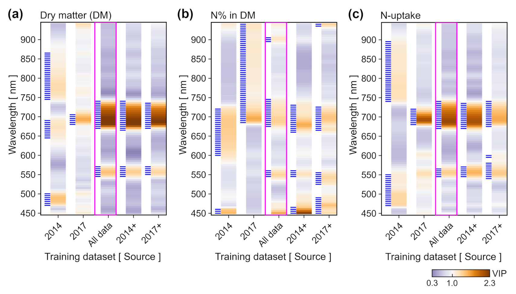
In addition to the estimation of grassland properties based on the complete hyperspectral dataset, the most important spectral features for prediction were identified and selected by calculating a confidence interval associated to $VIP$ values. This analysis revealed that feature importance for each trait varied between the different source datasets (2014 or 2017), indicating that the obtained models expressed different relationship between spectral information and grassland properties (Figure 7). This highlights the importance of calibration transfer approaches such as the one evaluated here, in particular for small datasets. Multivariate non-parametric models (such as PLSR) are mostly designed to minimize prediction errors for the training samples. This objective can lead to very good prediction accuracy for observations sharing the characteristics of the source domain. 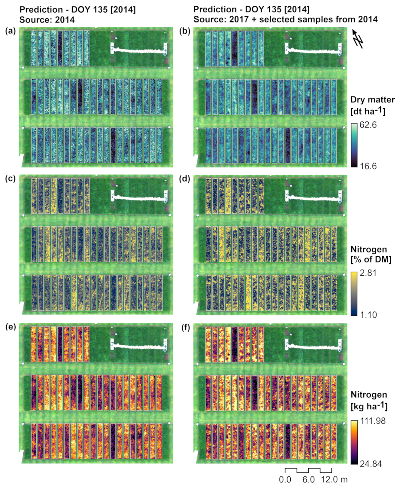However, the portability of such models to other conditions is questionable [12]. Inspecting the features selected after calibration transfer (i.e., after adding selected samples from the target domain to the training data) it is clear that a similar relationship between spectral information and traits was obtained for the different training datasets. 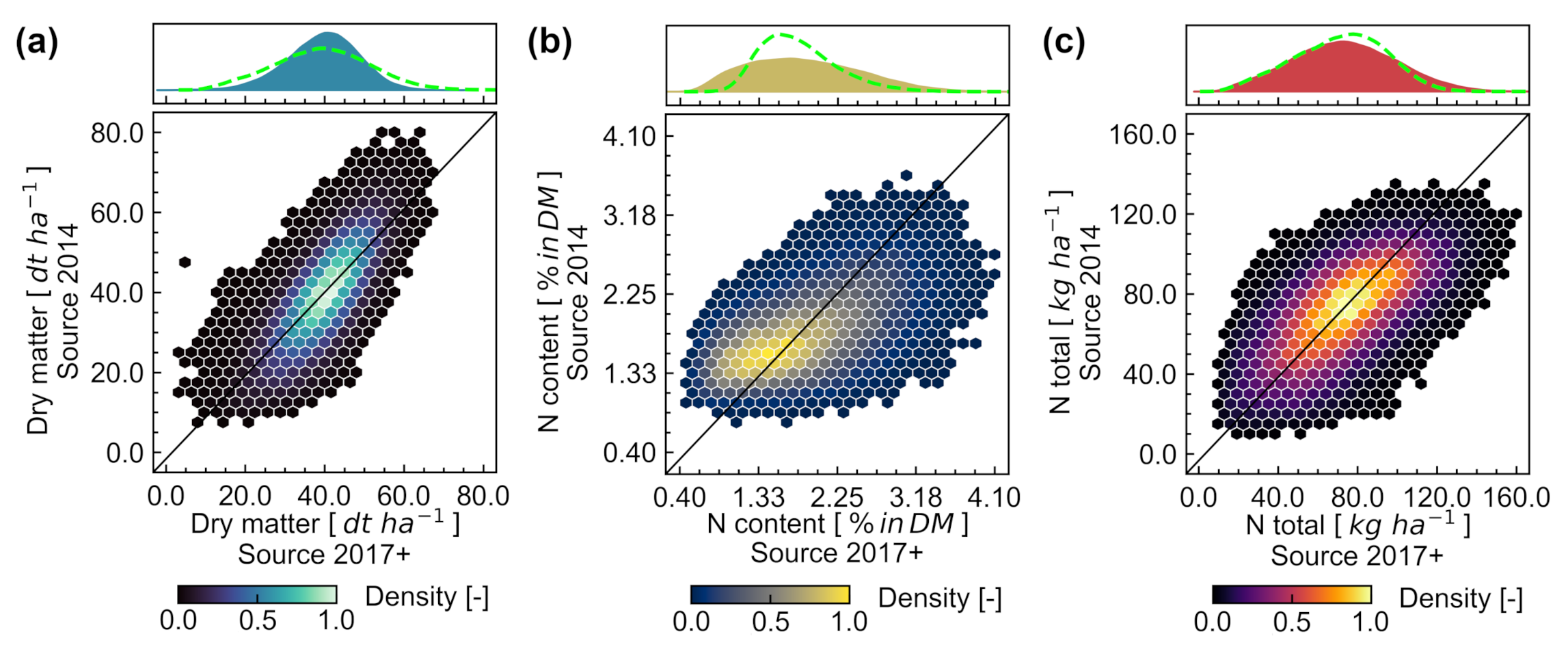Besides that, the similarity between maps (Figure 9 and Figure 10) derived from training data acquired the same year of the target date or from data collected in another year after transfer, indicate that the transferred models performed well for an individual date (15 May 2014, used as example), despite being more general. This resulted in pixel-wise representation of similar spatial patterns and overlap of marginal probability densities for values predicted in both cases.

5. Conclusions

In this study the retrieval of grassland traits based on multi-temporal UAV hyperspectral imagery was investigated. Special attention was given to model calibration transfer by selecting and adding samples from the target data to the training dataset. This procedure searched to adequately represent new observations, which was not possible based on the limited number of samples available before transfer. It was verified that accurate predictions of dry matter and N-related traits (N content in % of dry matter and N-uptake in kg ha${}^{-1}$) was possible using models derived from data acquired on the same year of the target date or after adding informative samples from the target date to a training dataset acquired in another year. By adding only a limited number of samples from the target date to a pre-existing dataset it was possible to reduce the number of samples that would need to be collected and analysed in a laboratory by up to 77%, depending on the trait of interest. In addition, $RMSE$ values for optimal transfer sets (i.e., identified after validation and used as benchmark) were only 20–30% lower than those obtained after model transfer based on prediction uncertainty, which represents an acceptable loss in accuracy depending on the objectives of the survey. These are important conclusions since grassland monitoring frameworks should be affordable in order to provide effective contribution to management practices. Vegetation sampling and laboratory analyses are laborious and costly tasks that may hamper the use of UAV-based monitoring systems to guide grassland management practices. Therefore, informative sample selection might provide an alternative to make monitoring frameworks more accessible, helping with their implementation in practice. Other options for grassland traits retrieval with greater generalization potential may involve RTM inversion approaches. While these solutions are based on sound research and involve state-of-art methods their application can eventually result in sub-optimal performance, in particular for systems that are complex and more difficult to characterize such as grass swards composed by multiple species and grass-legumes mixtures. In this sense, the results presented in our study demonstrate the potential of relatively simple methods and small datasets for the initial development and implementation of grassland monitoring solutions based on UAV hyperspectral datasets. Despite that, further research in this topic is certainly needed to develop more advanced approaches and/or compare the performance of different methods in order to offer adequate solutions for different scenarios.

References

1. Higgins, S.; Schellberg, J.; Bailey, J. Improving productivity and increasing the efficiency of soil nutrient management on grassland farms in the UK and Ireland using precision agriculture technology. Eur. J. Agron. 2019, 106, 67–74. [Google Scholar] [CrossRef]
2. Viljanen, N.; Honkavaara, E.; Näsi, R.; Hakala, T.; Niemeläinen, O.; Kaivosoja, J. A Novel Machine Learning Method for Estimating Biomass of Grass Swards Using a Photogrammetric Canopy Height Model, Images and Vegetation Indices Captured by a Drone. Agriculture 2018, 8, 70. [Google Scholar] [CrossRef] [Green Version]
3. Oenema, J.; van Ittersum, M.; van Keulen, H. Improving nitrogen management on grassland on commercial pilot dairy farms in the Netherlands. Agric. Ecosyst. Environ. 2012, 162, 116–126. [Google Scholar] [CrossRef]
4. Reynolds, D.; Baret, F.; Welcker, C.; Bostrom, A.; Ball, J.; Cellini, F.; Lorence, A.; Chawade, A.; Khafif, M.; Noshita, K.; et al. What is cost-efficient phenotyping? Optimizing costs for different scenarios. Plant Sci. 2019, 282, 14–22. [Google Scholar] [CrossRef] [PubMed] [Green Version]
5. Weiss, M.; Jacob, F.; Duveiller, G. Remote sensing for agricultural applications: A meta-review. Remote Sens. Environ. 2020, 236, 111402. [Google Scholar] [CrossRef]
6. Berger, K.; Verrelst, J.; Féret, J.B.; Wang, Z.; Wocher, M.; Strathmann, M.; Danner, M.; Mauser, W.; Hank, T. Crop nitrogen monitoring: Recent progress and principal developments in the context of imaging spectroscopy missions. Remote Sens. Environ. 2020, 242, 111758. [Google Scholar] [CrossRef]
7. Jenal, A.; Lussem, U.; Bolten, A.; Gnyp, M.L.; Schellberg, J.; Jasper, J.; Bongartz, J.; Bareth, G. Investigating the Potential of a Newly Developed UAV-based VNIR/SWIR Imaging System for Forage Mass Monitoring. PFG–J. Photogramm. Remote Sens. Geoinf. Sci. 2020, 88, 493–507. [Google Scholar] [CrossRef]
8. Pranga, J.; Borra-Serrano, I.; Aper, J.; De Swaef, T.; Ghesquiere, A.; Quataert, P.; Roldán-Ruiz, I.; Janssens, I.A.; Ruysschaert, G.; Lootens, P. Improving Accuracy of Herbage Yield Predictions in Perennial Ryegrass with UAV-Based Structural and Spectral Data Fusion and Machine Learning. Remote Sens. 2021, 13, 3459. [Google Scholar] [CrossRef]
9. Théau, J.; Lauzier-Hudon, E.; Aubé, L.; Devillers, N. Estimation of forage biomass and vegetation cover in grasslands using UAV imagery. PLoS ONE 2021, 16, e0245784. [Google Scholar] [CrossRef]
10. Capolupo, A.; Kooistra, L.; Berendonk, C.; Boccia, L.; Suomalainen, J. Estimating Plant Traits of Grasslands from UAV-Acquired Hyperspectral Images: A Comparison of Statistical Approaches. ISPRS Int. J. Geo-Inf. 2015, 4, 2792–2820. [Google Scholar] [CrossRef]
11. Grüner, E.; Astor, T.; Wachendorf, M. Prediction of Biomass and N Fixation of Legume–Grass Mixtures Using Sensor Fusion. Front. Plant Sci. 2021, 11, 603921. [Google Scholar] [CrossRef] [PubMed]
12. Verrelst, J.; Camps-Valls, G.; Muñoz-Marí, J.; Rivera, J.P.; Veroustraete, F.; Clevers, J.G.; Moreno, J. Optical remote sensing and the retrieval of terrestrial vegetation bio-geophysical properties—A review. ISPRS J. Photogramm. Remote Sens. 2015, 108, 273–290. [Google Scholar] [CrossRef]
13. Tuia, D.; Persello, C.; Bruzzone, L. Domain Adaptation for the Classification of Remote Sensing Data: An Overview of Recent Advances. IEEE Geosci. Remote Sens. Mag. 2016, 4, 41–57. [Google Scholar] [CrossRef]
14. Settles, B. Active Learning; Number 18 in Synthesis Lectures on Artificial Intelligence and Machine Learning; Morgan & Claypool Publishers: San Rafael, CA, USA, 2012. [Google Scholar]
15. Wu, D. Pool-Based Sequential Active Learning for Regression. IEEE Trans. Neural Netw. Learn. Syst. 2019, 30, 1348–1359. [Google Scholar] [CrossRef] [Green Version]
16. Berger, K.; Rivera Caicedo, J.P.; Martino, L.; Wocher, M.; Hank, T.; Verrelst, J. A Survey of Active Learning for Quantifying Vegetation Traits from Terrestrial Earth Observation Data. Remote Sens. 2021, 13, 287. [Google Scholar] [CrossRef]
17. Douak, F.; Melgani, F.; Benoudjit, N. Kernel ridge regression with active learning for wind speed prediction. Appl. Energy 2013, 103, 328–340. [Google Scholar] [CrossRef]
18. Wu, D.; Lin, C.T.; Huang, J. Active Learning for Regression Using Greedy Sampling. arXiv 2018, arXiv:1808.04245. [Google Scholar] [CrossRef] [Green Version]
19. Liu, Z.; Jiang, X.; Luo, H.; Fang, W.; Liu, J.; Wu, D. Pool-based unsupervised active learning for regression using iterative representativeness-diversity maximization (iRDM). Pattern Recognit. Lett. 2021, 142, 11–19. [Google Scholar] [CrossRef]
20. Panknin, D.; Müller, K.R.; Nakajima, S. Optimal Sampling Density for Nonparametric Regression. arXiv 2021, arXiv:2105.11990. [Google Scholar]
21. Suomalainen, J.; Anders, N.; Iqbal, S.; Roerink, G.; Franke, J.; Wenting, P.; Hünniger, D.; Bartholomeus, H.; Becker, R.; Kooistra, L. A Lightweight Hyperspectral Mapping System and Photogrammetric Processing Chain for Unmanned Aerial Vehicles. Remote Sens. 2014, 6, 11013–11030. [Google Scholar] [CrossRef] [Green Version]
22. Schläpfer, D.; Richter, R. Geo-atmospheric processing of airborne imaging spectrometry data. Part 1: Parametric orthorectification. Int. J. Remote Sens. 2002, 23, 2609–2630. [Google Scholar] [CrossRef]
23. James, M.; Robson, S.; d’Oleire Oltmanns, S.; Niethammer, U. Optimising UAV topographic surveys processed with structure-from-motion: Ground control quality, quantity and bundle adjustment. Geomorphology 2017, 280, 51–66. [Google Scholar] [CrossRef] [Green Version]
24. Honkavaara, E.; Rosnell, T.; Oliveira, R.; Tommaselli, A. Band registration of tuneable frame format hyperspectral UAV imagers in complex scenes. ISPRS J. Photogramm. Remote Sens. 2017, 134, 96–109. [Google Scholar] [CrossRef]
25. Singh, A.; Serbin, S.P.; McNeil, B.E.; Kingdon, C.C.; Townsend, P.A. Imaging spectroscopy algorithms for mapping canopy foliar chemical and morphological traits and their uncertainties. Ecol. Appl. 2015, 25, 2180–2197. [Google Scholar] [CrossRef] [Green Version]
26. Wang, Z.; Townsend, P.A.; Schweiger, A.K.; Couture, J.J.; Singh, A.; Hobbie, S.E.; Cavender-Bares, J. Mapping foliar functional traits and their uncertainties across three years in a grassland experiment. Remote Sens. Environ. 2019, 221, 405–416. [Google Scholar] [CrossRef]
27. Verrelst, J.; Dethier, S.; Rivera, J.P.; Munoz-Mari, J.; Camps-Valls, G.; Moreno, J. Active Learning Methods for Efficient Hybrid Biophysical Variable Retrieval. IEEE Geosci. Remote Sens. Lett. 2016, 13, 1012–1016. [Google Scholar] [CrossRef]
28. Chong, I.G.; Jun, C.H. Performance of some variable selection methods when multicollinearity is present. Chemom. Intell. Lab. Syst. 2005, 78, 103–112. [Google Scholar] [CrossRef]
29. Farrés, M.; Platikanov, S.; Tsakovski, S.; Tauler, R. Comparison of the variable importance in projection (VIP) and of the selectivity ratio (SR) methods for variable selection and interpretation: Comparison of variable selection methods. J. Chemom. 2015, 29, 528–536. [Google Scholar] [CrossRef]
30. Afanador, N.; Tran, T.; Buydens, L. An assessment of the jackknife and bootstrap procedures on uncertainty estimation in the variable importance in the projection metric. Chemom. Intell. Lab. Syst. 2014, 137, 162–172. [Google Scholar] [CrossRef]
31. Grüner, E.; Wachendorf, M.; Astor, T. The potential of UAV-borne spectral and textural information for predicting aboveground biomass and N fixation in legume-grass mixtures. PLoS ONE 2020, 15, 0234703. [Google Scholar] [CrossRef]
32. Michez, A.; Philippe, L.; David, K.; Sébastien, C.; Christian, D.; Bindelle, J. Can Low-Cost Unmanned Aerial Systems Describe the Forage Quality Heterogeneity? Insight from a Timothy Pasture Case Study in Southern Belgium. Remote Sens. 2020, 12, 1650. [Google Scholar] [CrossRef]
33. Oliveira, R.A.; Näsi, R.; Niemeläinen, O.; Nyholm, L.; Alhonoja, K.; Kaivosoja, J.; Jauhiainen, L.; Viljanen, N.; Nezami, S.; Markelin, L.; et al. Machine learning estimators for the quantity and quality of grass swards used for silage production using drone-based imaging spectrometry and photogrammetry. Remote Sens. Environ. 2020, 246, 111830. [Google Scholar] [CrossRef]
34. Wijesingha, J.; Astor, T.; Schulze-Brüninghoff, D.; Wengert, M.; Wachendorf, M. Predicting Forage Quality of Grasslands Using UAV-Borne Imaging Spectroscopy. Remote Sens. 2020, 12, 126. [Google Scholar] [CrossRef] [Green Version]
35. Askari, M.S.; McCarthy, T.; Magee, A.; Murphy, D.J. Evaluation of Grass Quality under Different Soil Management Scenarios Using Remote Sensing Techniques. Remote Sens. 2019, 11, 1835. [Google Scholar] [CrossRef] [Green Version]
36. Schucknecht, A.; Seo, B.; Krämer, A.; Asam, S.; Atzberger, C.; Kiese, R. Estimating dry biomass and plant nitrogen concentration in pre-Alpine grasslands with low-cost UAS-borne multispectral data—A comparison of sensors, algorithms, and predictor sets. Biogeosci. Discuss. 2021, 1–39. [Google Scholar] [CrossRef]
37. Obermeier, W.; Lehnert, L.; Pohl, M.; Makowski Gianonni, S.; Silva, B.; Seibert, R.; Laser, H.; Moser, G.; Müller, C.; Luterbacher, J.; et al. Grassland ecosystem services in a changing environment: The potential of hyperspectral monitoring. Remote Sens. Environ. 2019, 232, 111273. [Google Scholar] [CrossRef]
38. Geipel, J.; Bakken, A.K.; Jørgensen, M.; Korsaeth, A. Forage yield and quality estimation by means of UAV and hyperspectral imaging. Precis. Agric. 2021, 22, 1437–1463. [Google Scholar] [CrossRef]
39. Zhuang, F.; Qi, Z.; Duan, K.; Xi, D.; Zhu, Y.; Zhu, H.; Xiong, H.; He, Q. A Comprehensive Survey on Transfer Learning. Proc. IEEE 2021, 109, 43–76. [Google Scholar] [CrossRef]
40. Mishra, P.; Nikzad-Langerodi, R.; Marini, F.; Roger, J.M.; Biancolillo, A.; Rutledge, D.N.; Lohumi, S. Are standard sample measurements still needed to transfer multivariate calibration models between near-infrared spectrometers? The answer is not always. TrAC Trends Anal. Chem. 2021, 143, 116331. [Google Scholar] [CrossRef]
41. Verrelst, J.; Berger, K.; Rivera-Caicedo, J.P. Intelligent Sampling for Vegetation Nitrogen Mapping Based on Hybrid Machine Learning Algorithms. IEEE Geosci. Remote Sens. Lett. 2020, 1–5. [Google Scholar] [CrossRef]
42. Wan, L.; Cen, H.; Zhu, J.; Zhang, J.; Zhu, Y.; Sun, D.; Du, X.; Zhai, L.; Weng, H.; Li, Y.; et al. Grain yield prediction of rice using multi-temporal UAV-based RGB and multispectral images and model transfer—A case study of small farmlands in the South of China. Agric. For. Meteorol. 2020, 291, 108096. [Google Scholar] [CrossRef]
43. Kooistra, L.; Franceschini, M.H.D.; Becker, R.; Wichern, F.; Suomalainen, J.; Bartholomeus, H.; Capolupo, A. Haus Riswick Grassland Experiment with N Fertilization and Plant Growth Monitoring Based on Unmanned Aerial Vehicle (UAV) Hyperspectral Imagery—Campaigns of 2014 and 2017; Dataset; 4TU.ResearchData: Delft, The Netherlands, 2022. [Google Scholar] [CrossRef]
Figure 1. UAV dataset acquired on 9 May 2017 (Day of the Year—DOY 130). In (a), orthomosaic derived from RGB high-resolution images (with Ground Sampling Distance—GSD of 0.015 m), in the upper portion of the figure, and hyperspectral image corresponding to a single flight line (with GSD of 0.156 m), in the bottom. Crop Surface Model (CSM) derived using Structure from Motion (SfM) applied to the RGB images is represented in (b), which was used for geometric correction of the hyperspectral data (as described in Section 2.3). Boundaries of the experimental plots are represented by white lines in both figures (a,b) and red lines indicate areas of interest from which the spectral information was extracted.
Drones 06 00073 g001
Figure 2. Performance of PLSR models based on different source datasets for predictions of dry matter (a) and nitrogen related traits (N% in dry matter, (b); and N-uptake in kg ha 1 , (c)), considering validation samples from the same season (diagonal in the matrices) or from a different target season (outside the diagonals in the same row). Values in each cell correspond to R 2 and R M S E , which is given between brackets. R 2 is also represented through colours. R 2 and R M S E indicate the average for outputs from 100 random models. R M S E standard deviation is also provided, inside brackets (after ± signal). R M S E is expressed with respect to the interquartile range ( I Q R ) observed for each trait in the complete dataset (‘All data’; i.e., 10.80 dt ha 1 , 0.51% in DM and 21.57 kg ha 1 for dry matter, N-content and N-uptake, respectively).
Drones 06 00073 g002
Figure 3. Performance of PLSR models for prediction of dry matter (a,d) and nitrogen related traits (N% in dry matter, (b,e); and N-uptake in kg ha 1 , (c,f)), evaluated using independent validation samples. Blue bars indicate model accuracy when the target date well represented in the calibration dataset (same number of samples in comparison to the source dataset—benchmark scenario), while green bars correspond to model performance when samples from the source domain are just combined with a selection of samples from the target dataset (i.e., after calibration transfer). Bars represent average R 2 and R M S E for outputs from 100 random models and error bars indicate the corresponding standard deviation. The mode for the number of factors (NF) included in the PLSR models is indicated in brackets below the y-axis labels in (ac). R M S E is expressed with respect to the interquartile range ( I Q R ) observed for each trait in the complete dataset (see Figure 2). A gradual increase in the number of observations from the target domain used for model fitting is considered. Therefore, selected samples from the previous dates were always included in the training dataset, when applicable. Similarly, the validation dataset was also gradually updated, by adding new samples from the target dates. Red circles in (df) represent the ratio between R M S E for the optimal number of samples for transfer (lowest R M S E observed, indicated in Figure 4) and R M S E obtained with the number of samples judged as optimal based on sample diversity and prediction uncertainty (as described in Section 2.5, also indicated in Figure 4).
Drones 06 00073 g003
Figure 4. R M S E of validation (error bar center correspond to averages while extremities indicate ±1 std. interval) for dry matter (a) and nitrogen related traits (N% in dry matter, (b); and N-uptake in kg ha 1 , (c)), according to the number of samples from the target domain added to the training dataset. Up to half of the samples available for each target date were considered for model transfer. Bars in the orange frame above the graphs indicate which number of samples was optimal for each date (i.e., lowest R M S E values) and in the red frame which number was effectively selected following the diversity and prediction uncertainty criteria (as described in Section 2.5). It is worth noting that the validation dataset in each case includes samples from the source and target domains, until the date indicate by the error bar colour (see legend).
Drones 06 00073 g004
Figure 5. R M S E of validation (middle of error bar corresponds to average while extremities indicate ±1 std.) for predictions of dry matter (a) and N related traits (N% in dry matter, (b); and N-uptake in kg ha 1 , (c)) when transfer samples from the target domain are selected considering (y-axis) or not (x-axis) prediction uncertainty. Only the R M S E values obtained by adding the number of samples considered as optimal for transfer according to the uncertainty reduction criterium (described in Section 2.5 and indicated in Figure 4) were used for comparison.
Drones 06 00073 g005
Figure 6. Sample-wise prediction accuracy and uncertainty for dry matter (ac) and nitrogen related traits (N% in dry matter, (df); and N-uptake in kg ha 1 , (gi)). Results ( R 2 and R M S E ) correspond to the average outputs for 100 random training datasets derived via bootstrap. In (c,f,i) the training data was obtained by randomly selecting the same number of samples from each date (i.e., 70% of the observations available—benchmark dataset). In contrast (a,d,g) correspond to models trained using samples collected in 2014 as source (i.e., 70% of samples included in the training data) with additional samples from acquisition dates in 2017 (with optimal number for each target date selected by considering prediction uncertainty, see Figure 4). Similarly, for (b,e,h) the models were trained using samples collected in 2017 as source (i.e., 70% of samples included in the training data) with additional samples from acquisition dates in 2014 (with optimal number for each target date selected by considering the prediction uncertainty, see Figure 4). Error bar indicates prediction uncertainty for a given sample and colour represents the date of acquisition or if the sample was included in the validation dataset. Red dashed line indicates a linear fit over the validation results (average predictions against observed values). Continuous black line indicates the 1:1 relationship between observed and predicted values.
Drones 06 00073 g006
Figure 7. Average Variable Importance in the Projection ( V I P ) for each spectral band when used as predictor to estimate dry matter (a) and nitrogen related traits (N% in dry matter, (b); and N-uptake in kg ha 1 , (c)). In the first two columns from (ac), results correspond to models trained using only samples from a single year (2014 or 2017). In contrast, other columns represent models derived using samples from all dates. The difference is that in the third column both years contribute equally to the calibration dataset (i.e., 70% of samples available for each date—benchmark scenario; indicated in red) while for the last two columns in each graph samples from the target dataset were selected based on prediction uncertainty (the number of samples chosen in each case is indicated in Figure 4).
Drones 06 00073 g007
Figure 8. Sample-wise prediction accuracy and uncertainty for dry matter (ac) and nitrogen related traits (N% in dry matter, (df); and N-uptake in kg ha 1 , (gi)), after variable selection (see Figure 7). Results ( R 2 and R M S E ) correspond to the average outputs for 100 random training datasets derived via bootstrap. In (c,f,i) the training data was obtained by randomly selecting the same number of samples from each date (i.e., 70% of the observations available—benchmark dataset). In contrast (a,d,g) correspond to models trained using samples collected in 2014 as source (i.e., 70% of samples included in the training data) with additional samples from acquisition dates in 2017 (with optimal number for each target date selected by considering prediction uncertainty, see Figure 4). Similarly, for (b,e,h) models were trained using samples collected in 2017 as source (i.e., 70% of samples included in the training data) with additional samples from acquisition dates in 2014 (optimal number for each target date selected by considering prediction uncertainty, see Figure 4). Error bar indicates prediction uncertainty for a given sample and colour represents the date of acquisition or if the sample was included in the validation dataset. Red dashed line indicates a linear fit over the validation results (average predictions against observed values). Continuous black line indicates the 1:1 relationship between observed and predicted values.
Drones 06 00073 g008
Figure 9. Pixel-wise comparison for predictions of dry matter (a) and nitrogen related traits (N% in dry matter, (b); and N-uptake in kg ha 1 , (c)) derived from models trained using only samples from 2014 (y-axis) in contrast to those derived from data collected in 2017 after transfer (x-axis; i.e., after selected samples from the target dataset in 2014 were added to the calibration samples set from 2017). Predictions corresponds to all pixels extracted from images acquired on the 15 May 2014 (DOY 134), as illustrated in Figure 10. The frequency of occurrence for different pixel values (density) is represented by colours in a regular hexagonal grid and marginal probability densities are illustrated in the y-axis extremity for comparison (darker colours correspond to probability densities for predictions based on the transferred dataset—2017+, while green lines describe probability density for predictions made using only calibration samples from 2014). Hexagons with less than 5 pixels are not displayed.
Drones 06 00073 g009
Figure 10. Pixel-wise prediction of grassland traits (dry matter, (a,b); nitrogen content in % of dry matter, (c,d); and N-uptake in kg ha 1 , (e,f)) for the 15 May 2014 (DOY 135). In (a,c,e) predictions were made using models derived from training data comprising only samples from 2014 (i.e., 70% of samples available for DOY 135 and 288). On the other hand, (b,d,f) correspond to predictions obtained from models trained mainly on data acquired in 2017 (i.e., 70% of samples available for DOY 130, 242 and 299) combined with a selected number of samples from those available for the 15 May 2014 (target date; number of transfer samples chosen for each trait is indicated in Figure 4).
Drones 06 00073 g010
Publisher’s Note: MDPI stays neutral with regard to jurisdictional claims in published maps and institutional affiliations.