
Unstable Landing Platform Pose Estimation Based on Camera and Range Sensor Homogeneous Fusion (CRHF)


Abstract
:1. Introduction
1.1. Problem Statement
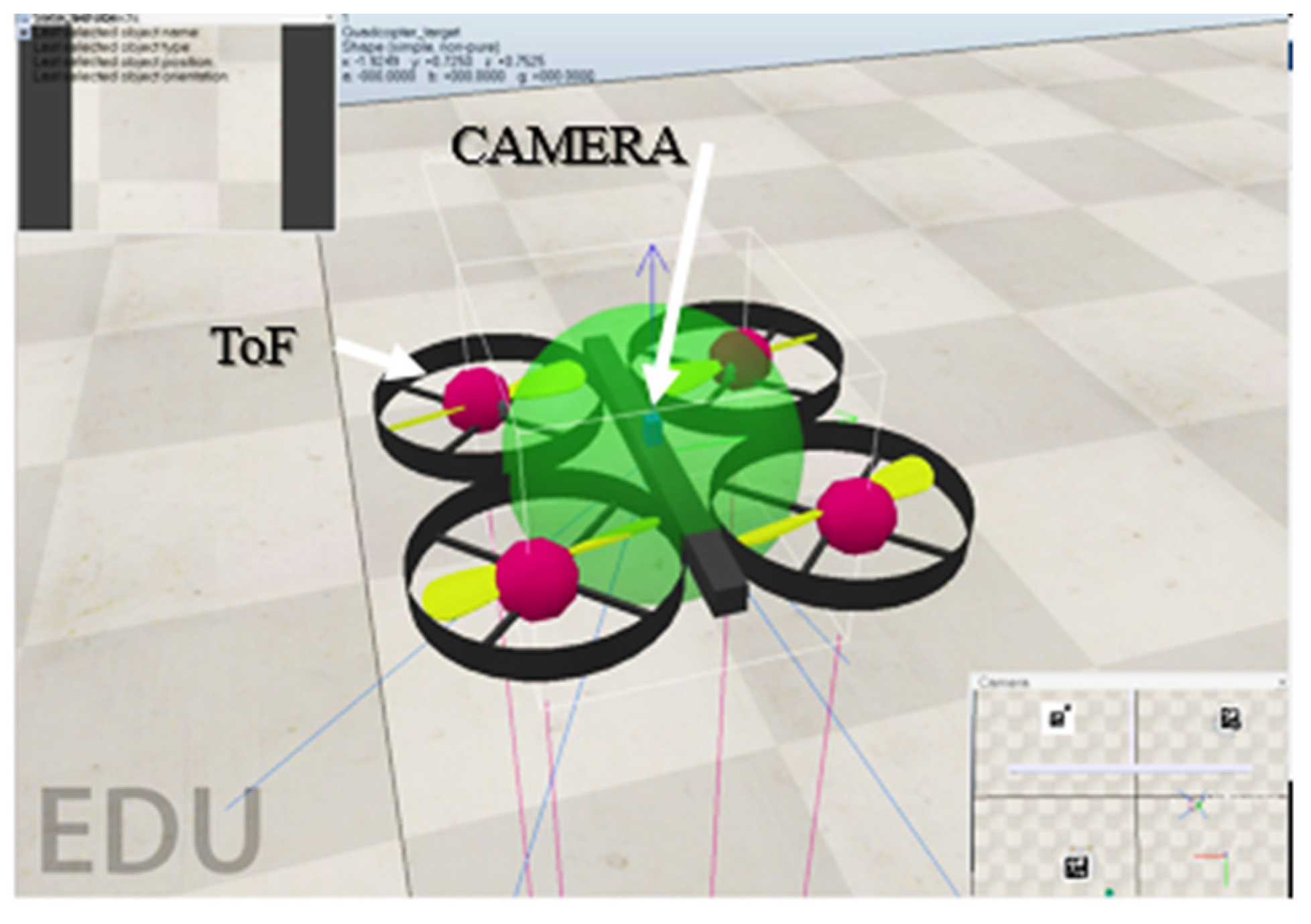
- The first contribution would be increasing the accuracy of altitude estimation during landing using range sensors, Time of Flight (ToF) sensors. This is a fit replacement for Light Detection and Ranging (LIDAR), which is expensive and heavy for installation on small-sized drones.
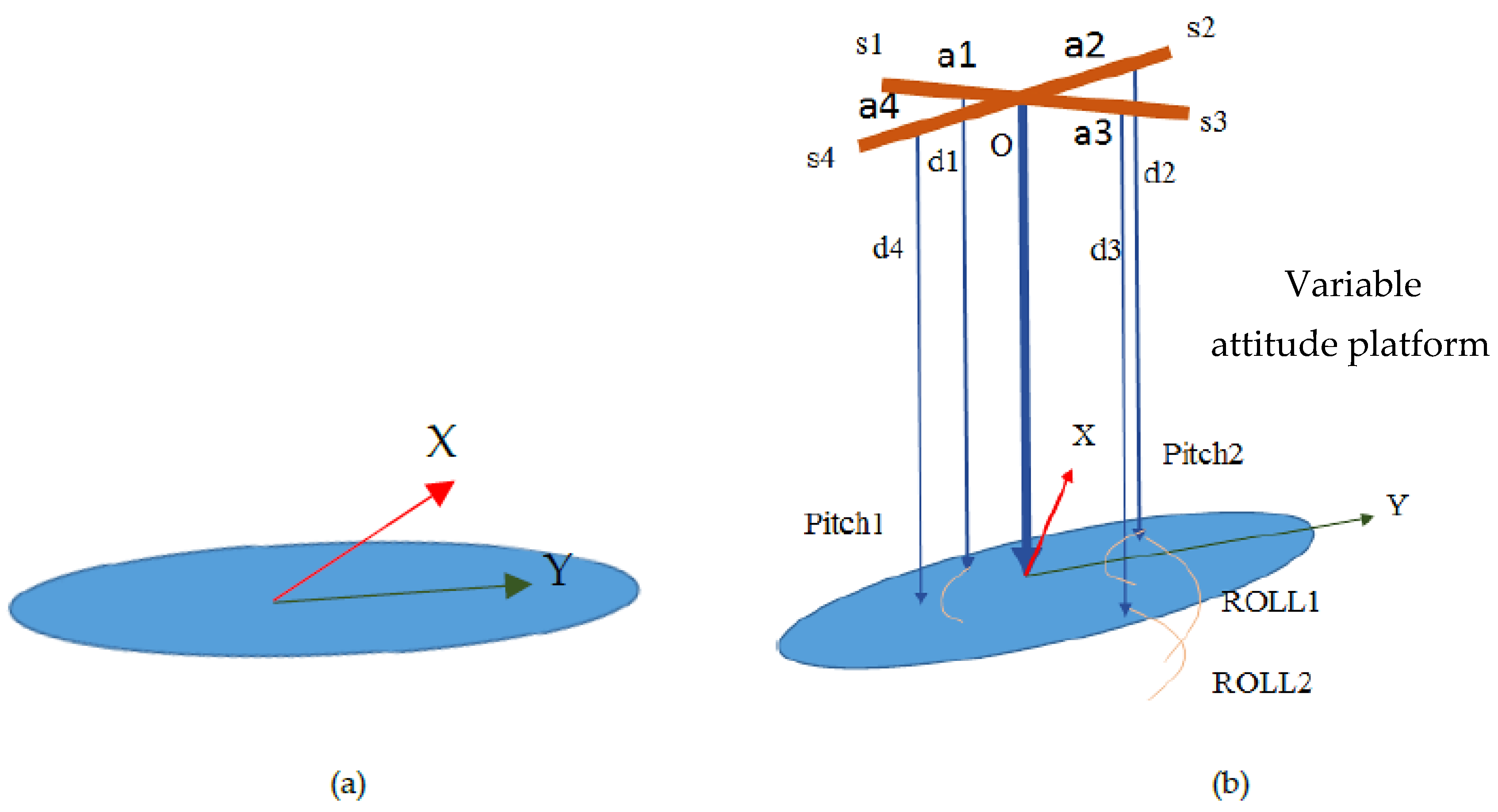
- Second, knowing the four ranges from the sensors, the equation of the descending platform is calculated. Hence, this ameliorates the calculation accuracy of the landing points in the real world in X and Y directions as well, letting X, Y, and Z be the world coordinate system.
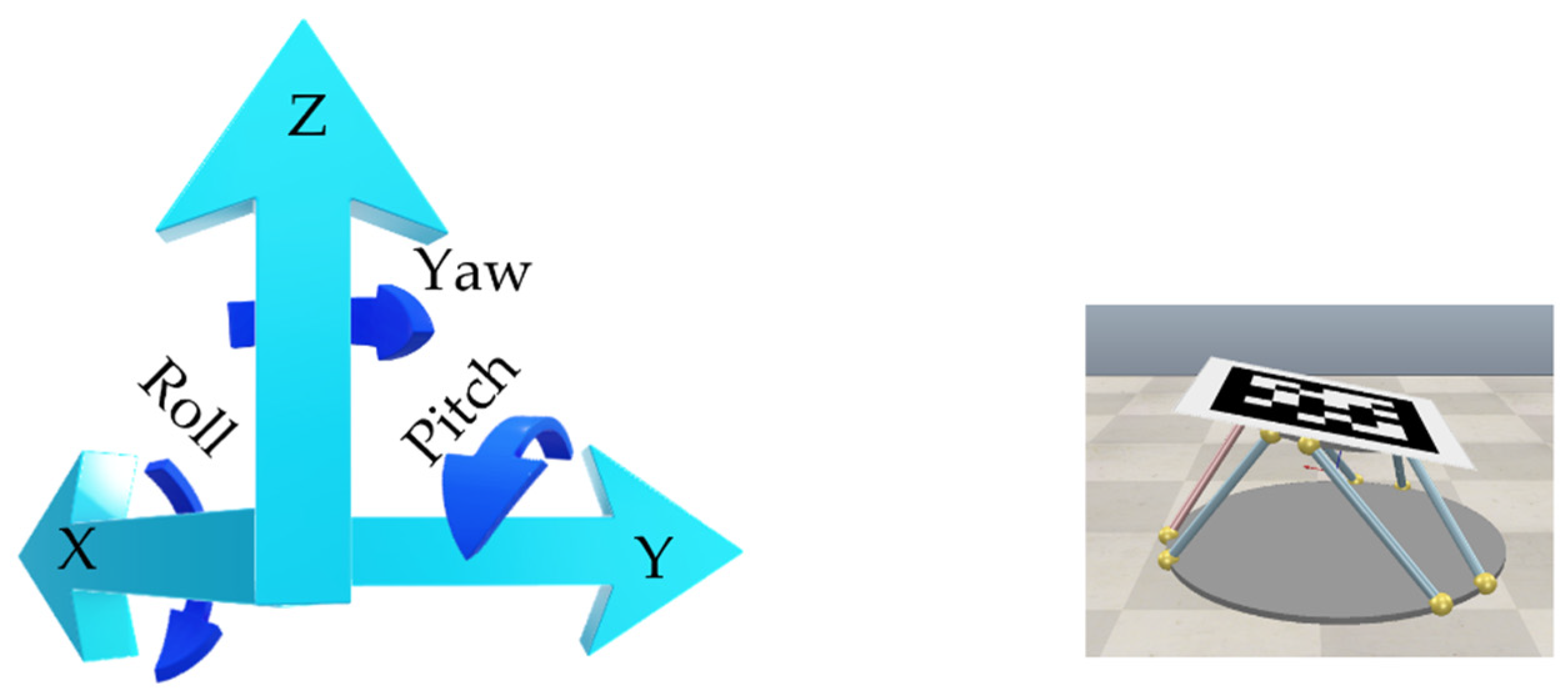
- The data from the range sensors are also used for the calculation of landing platform Euler angles. Therefore, the proposed algorithm improves Euler angle estimation.
- Lastly, we employed sensor fusion that can operate completely in low light conditions. The camera contributes to the calculation of the headings of the landing platform; hence, the algorithm can be used in situations when the heading calculation is insignificant.
1.2. Literature Review
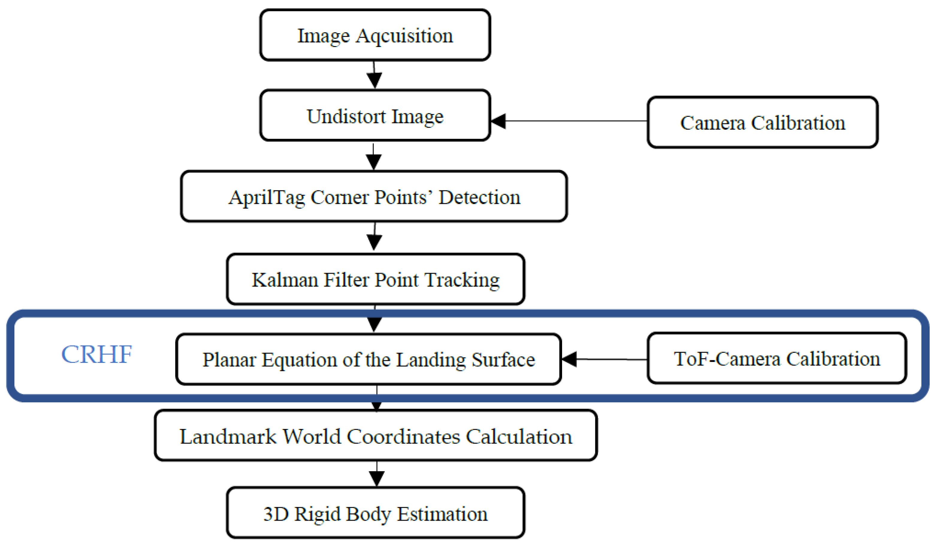
2. Proposing Camera and Range Sensor Homogeneous Fusion (CRHF)
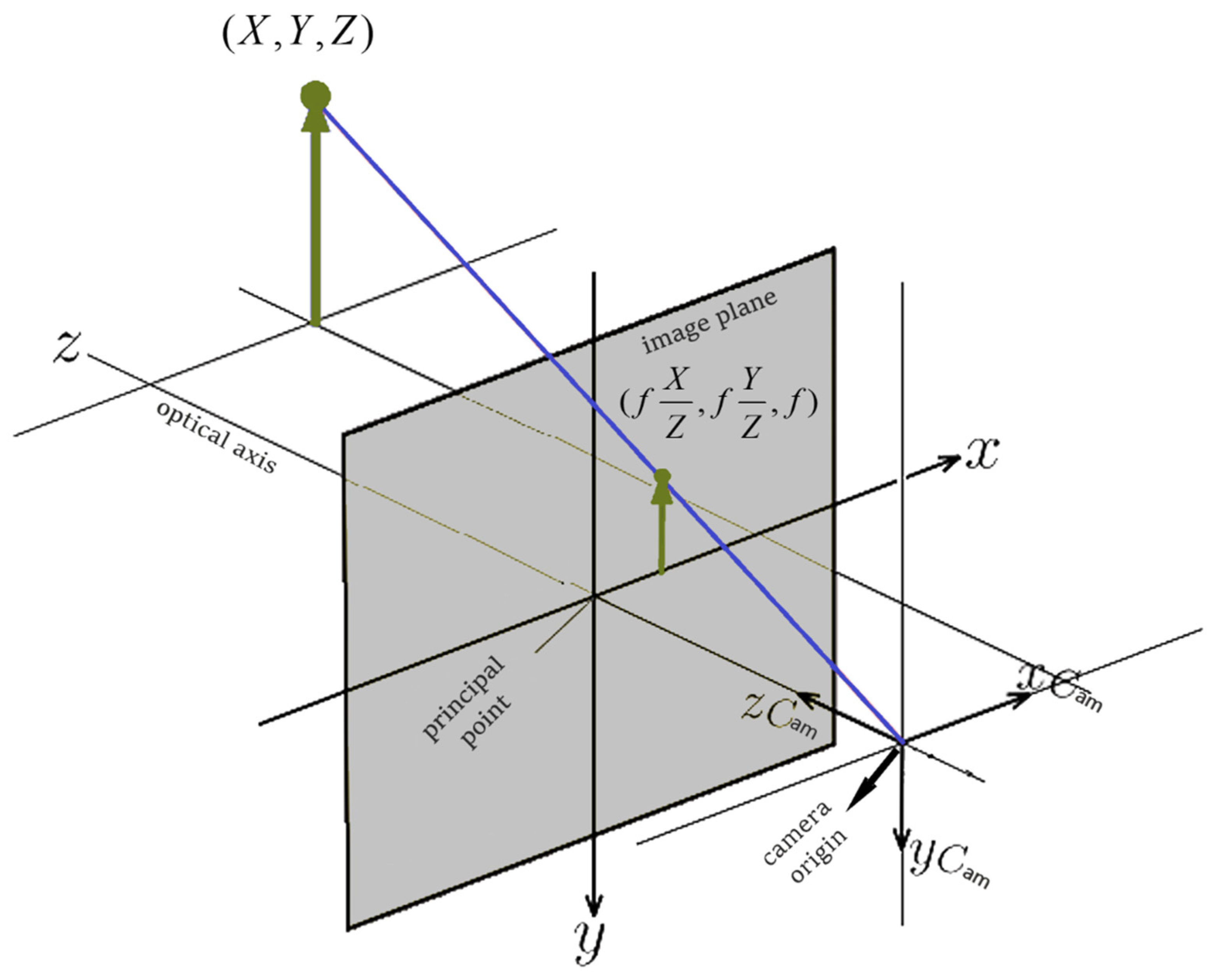
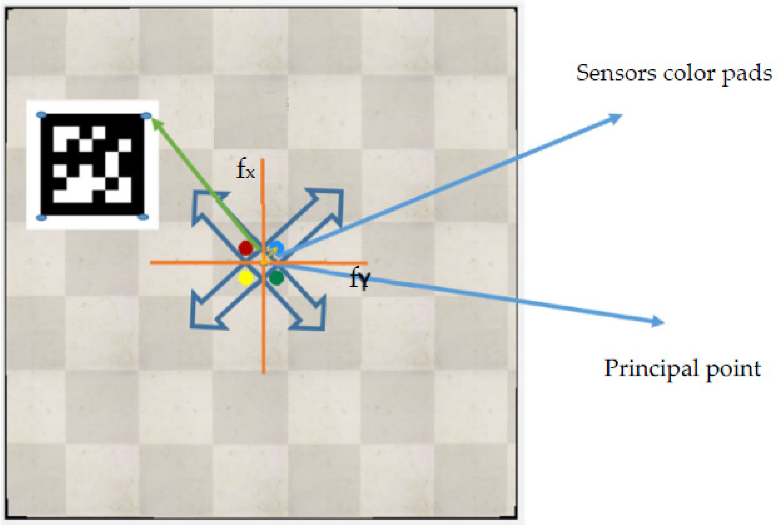
2.1. Camera Calibration
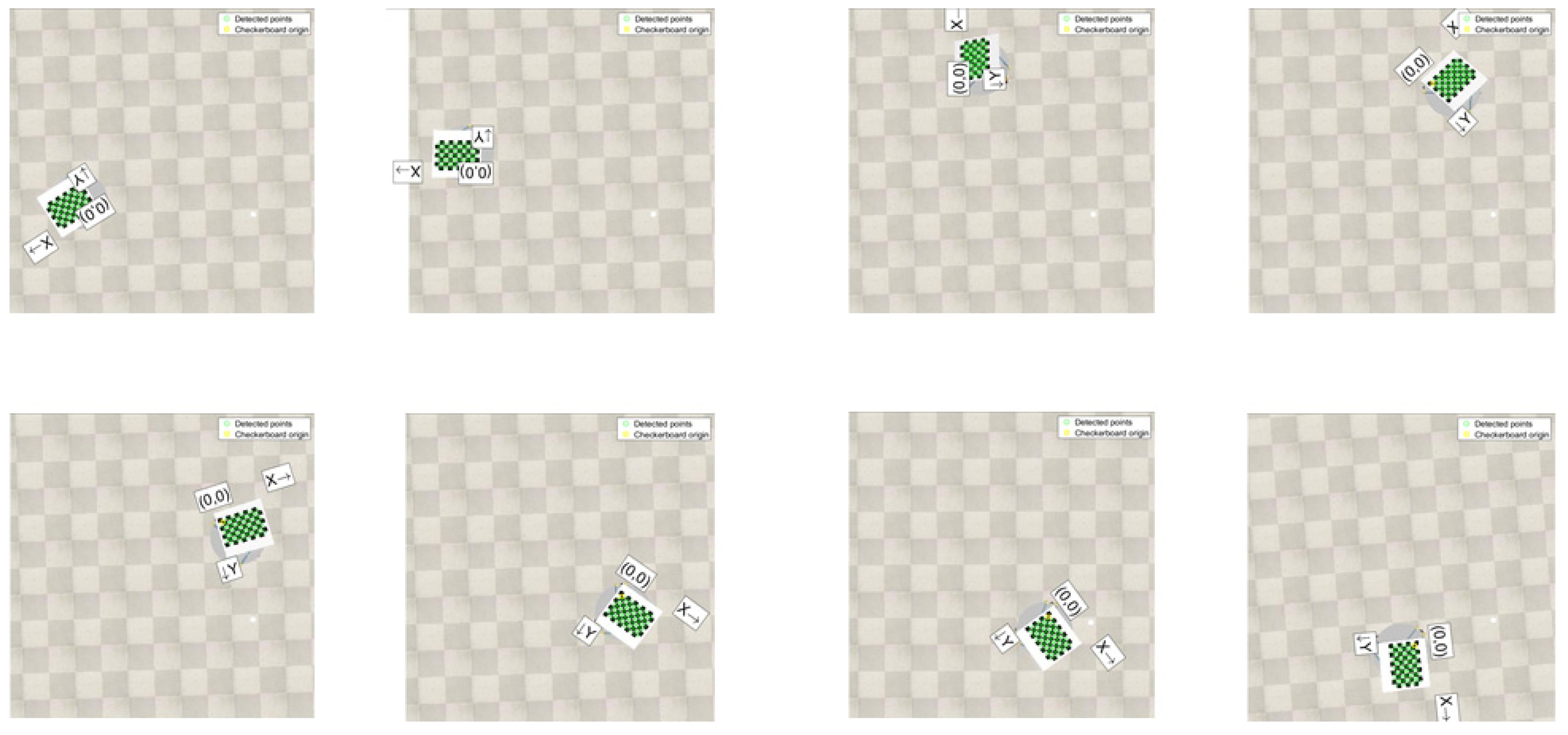
- Collect images;
- Convert them into a grayscale image;
- Calculate the chessboard corners from the grayscale image;
- Compute the real-word chessboard corners. The chessboard has a square size of 7 cm and 7 × 10 corners; and
- The input image point coordinates determined by transform “T” normalization;
- Camera projection matrix CN, camera matrix in frame number N, projected from the normalized image points;
- Camera matrix C as the CNT−1 denormalization;
- The reprojected image point coordinates, xE, calculated by C and X multiplication;
- Use the two equations below, (5) and (6), to obtain radial distortion coefficients of the camera [33,34].in which x and y are the coordinates of the normalized image—undistorted pixel position, is the coordinate of the distorted pixel in the x direction, is the coordinate of the distorted pixel in the y direction, and k1, k2, and k3 are the lens’s radial distortion coefficients. The magnitude of the radial distortion can be calculated as follows [35,36,37,38]:
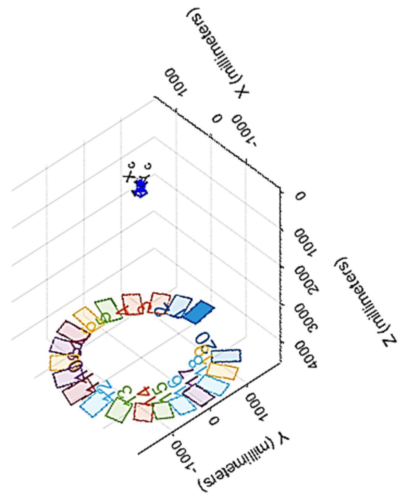
2.2. Camera Calibration Implementation and Results
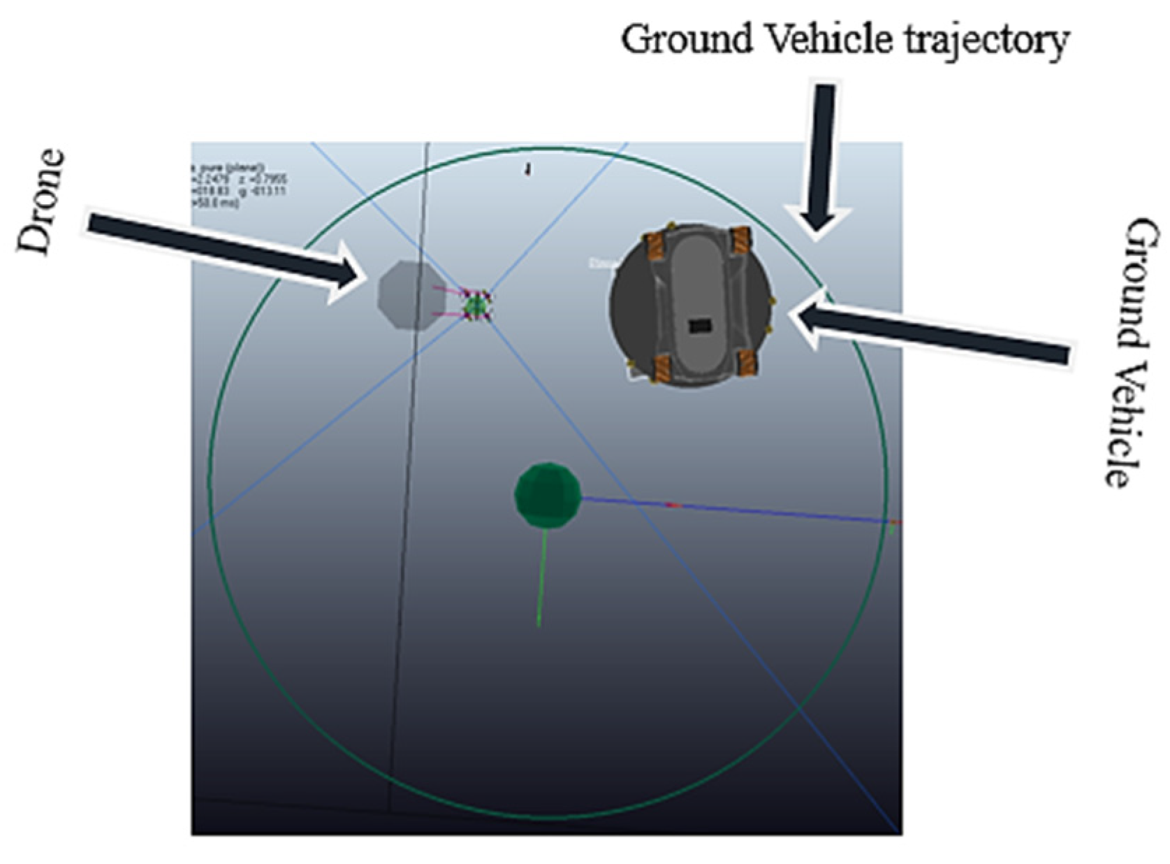
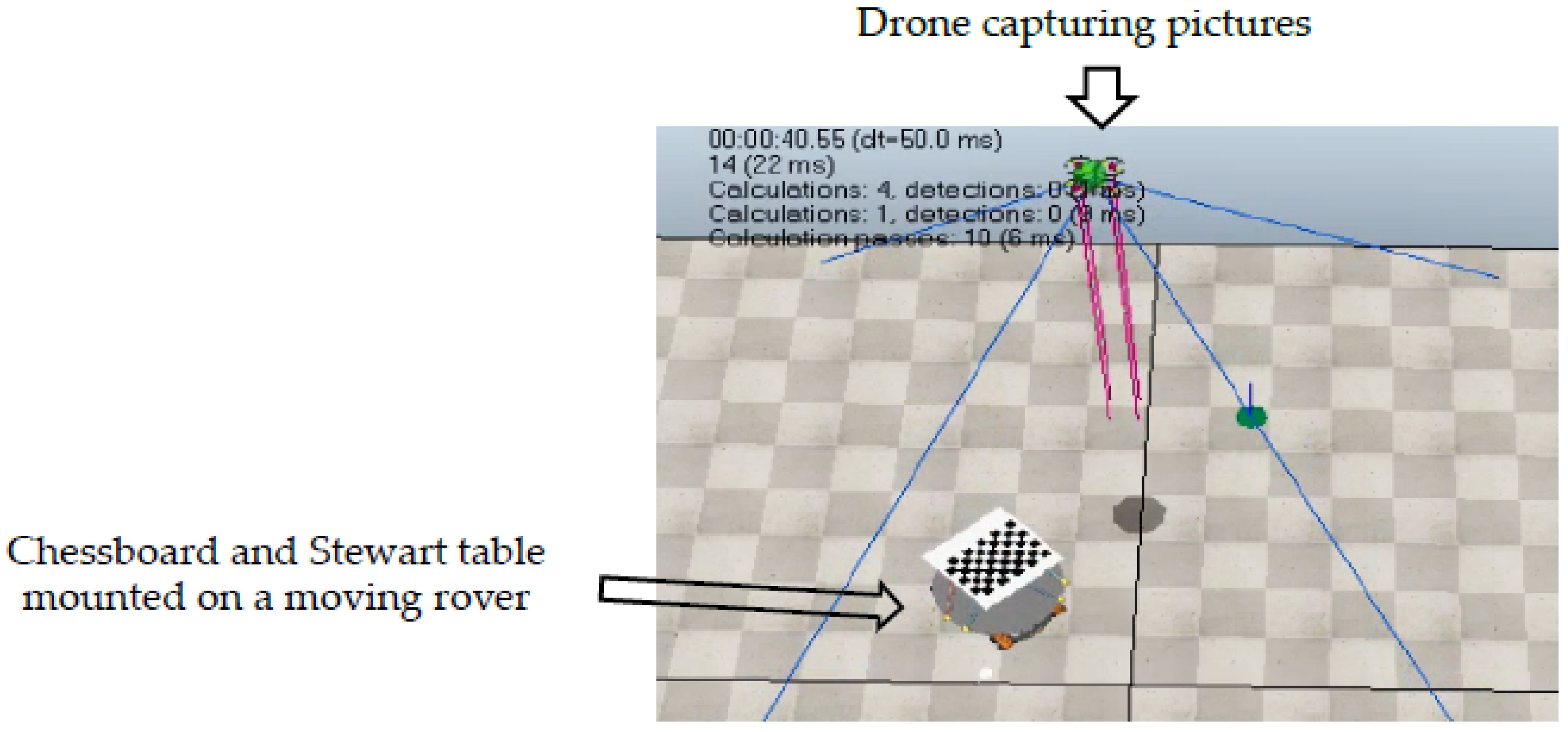
- The drone takes off.
- It hovers towards the surveillance point that includes all the rover paths and waits without any movement.
- The drone takes 20 photos when the rover is traveling along the circular path.
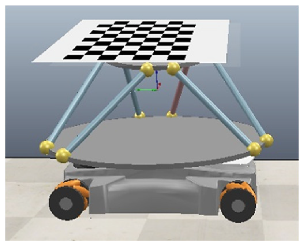
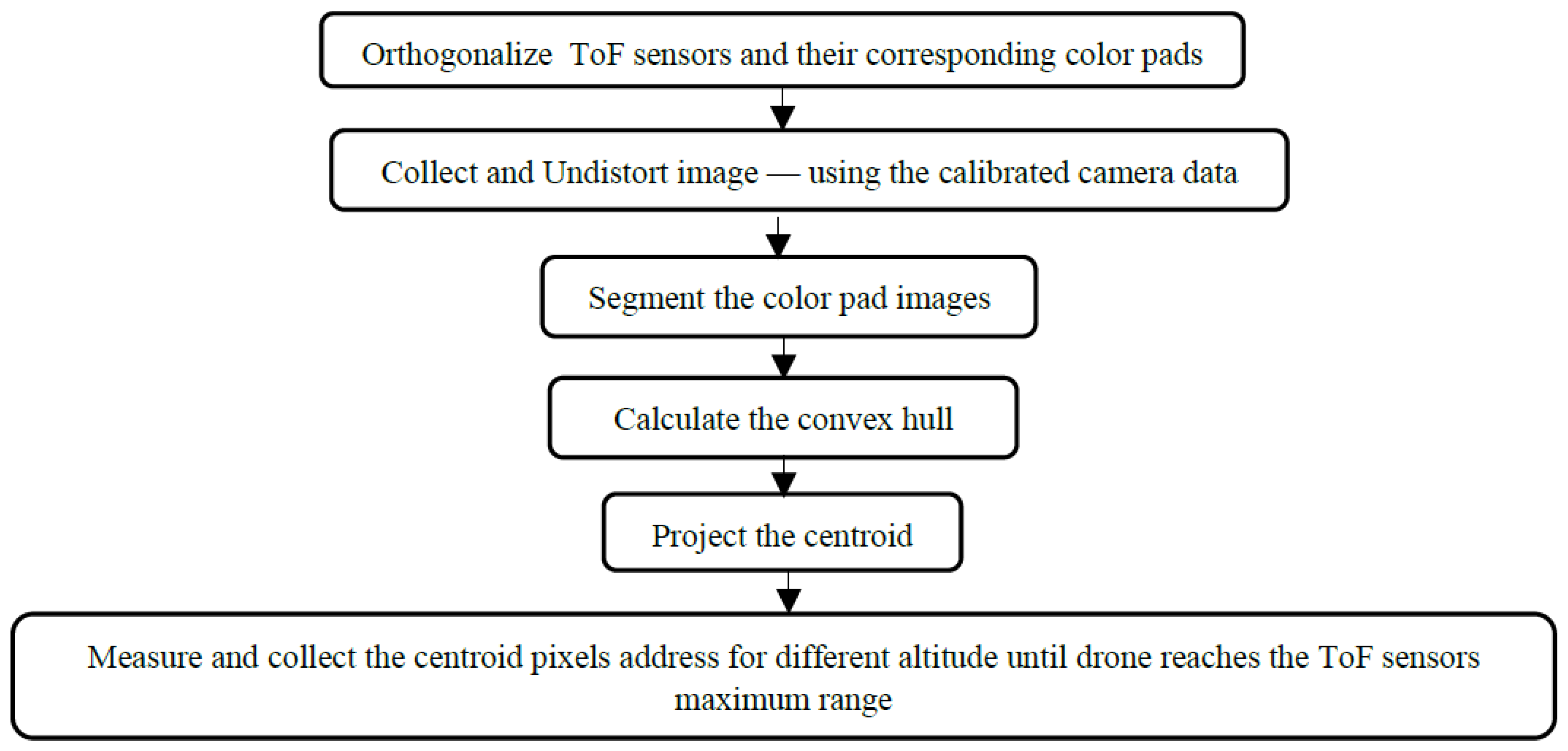
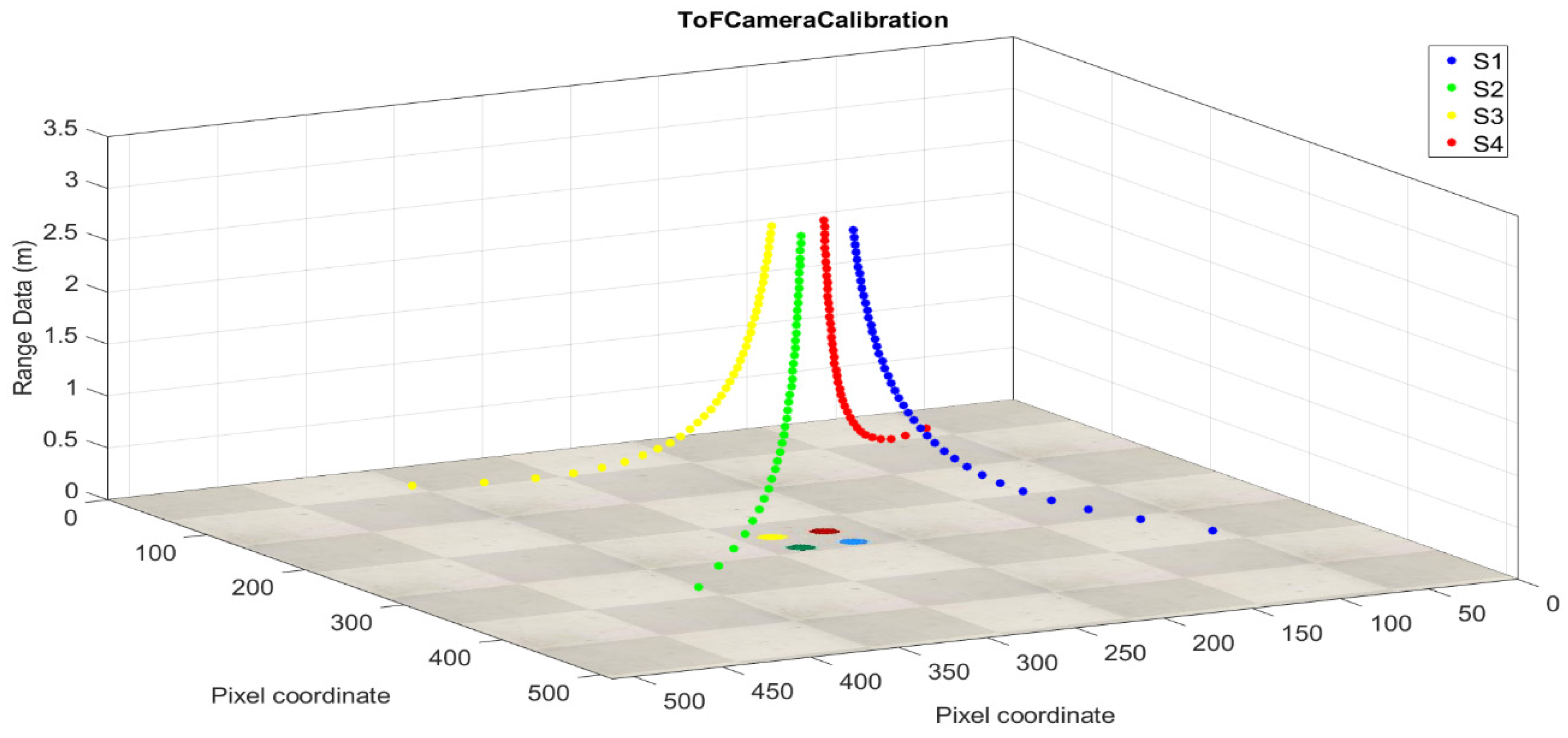
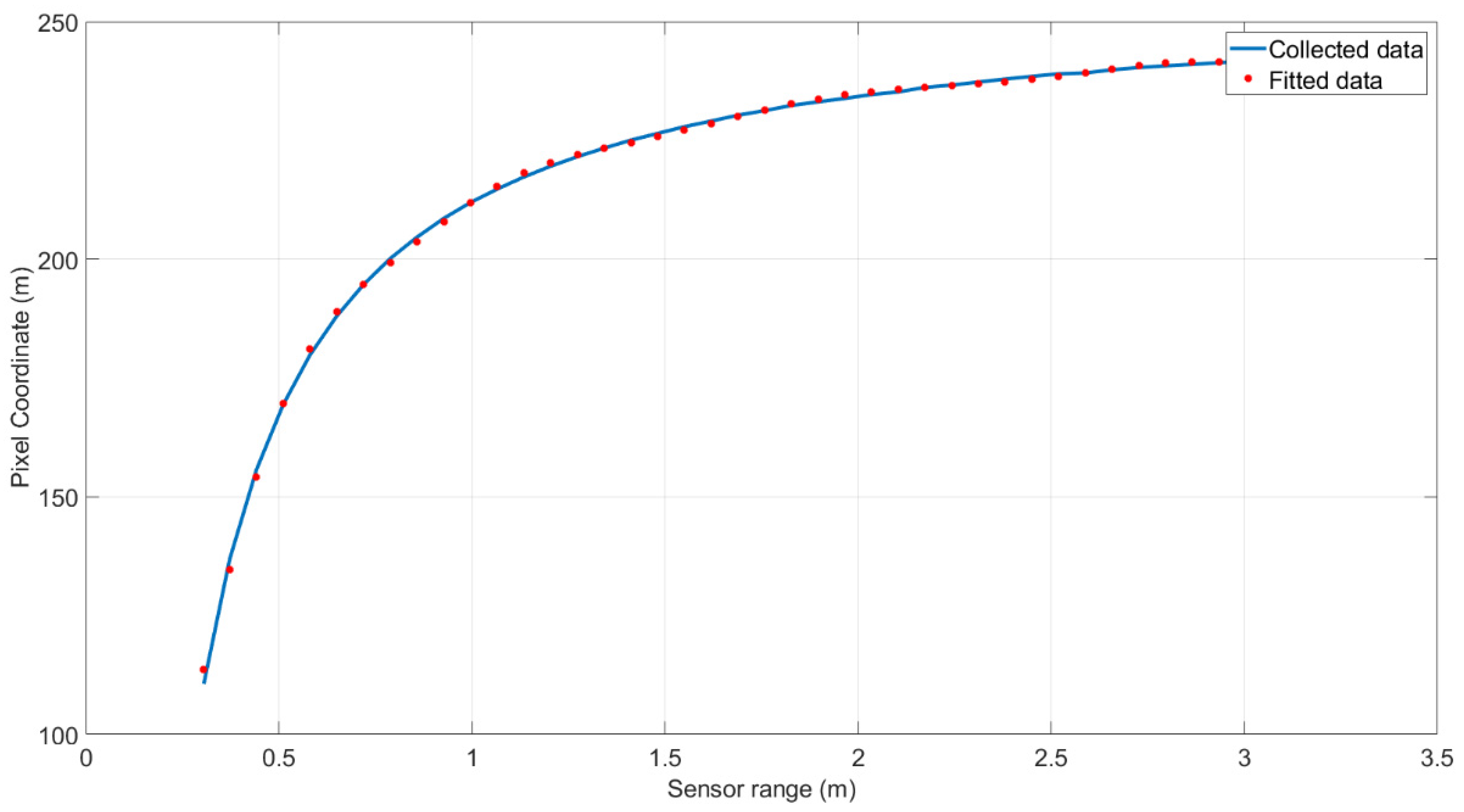
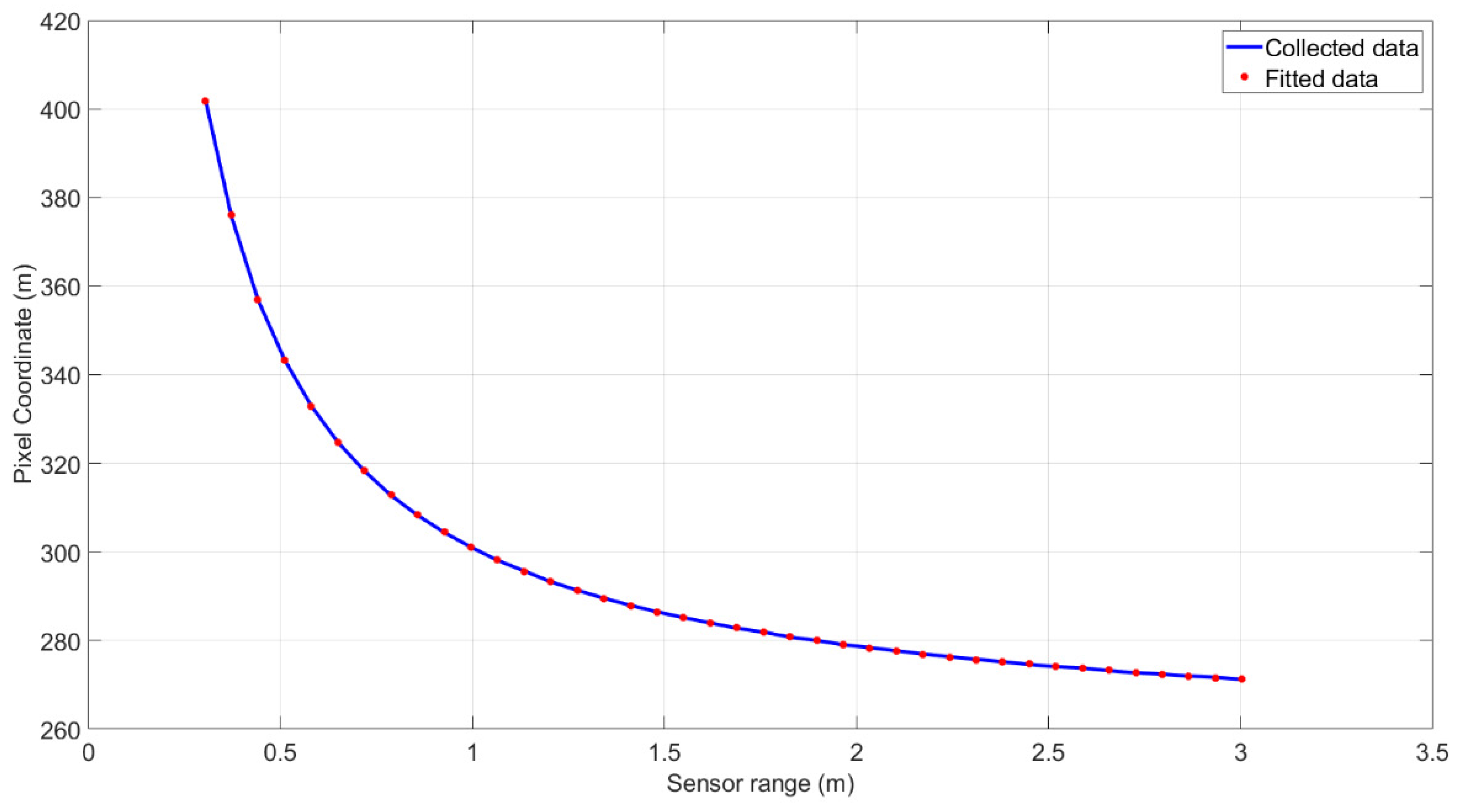
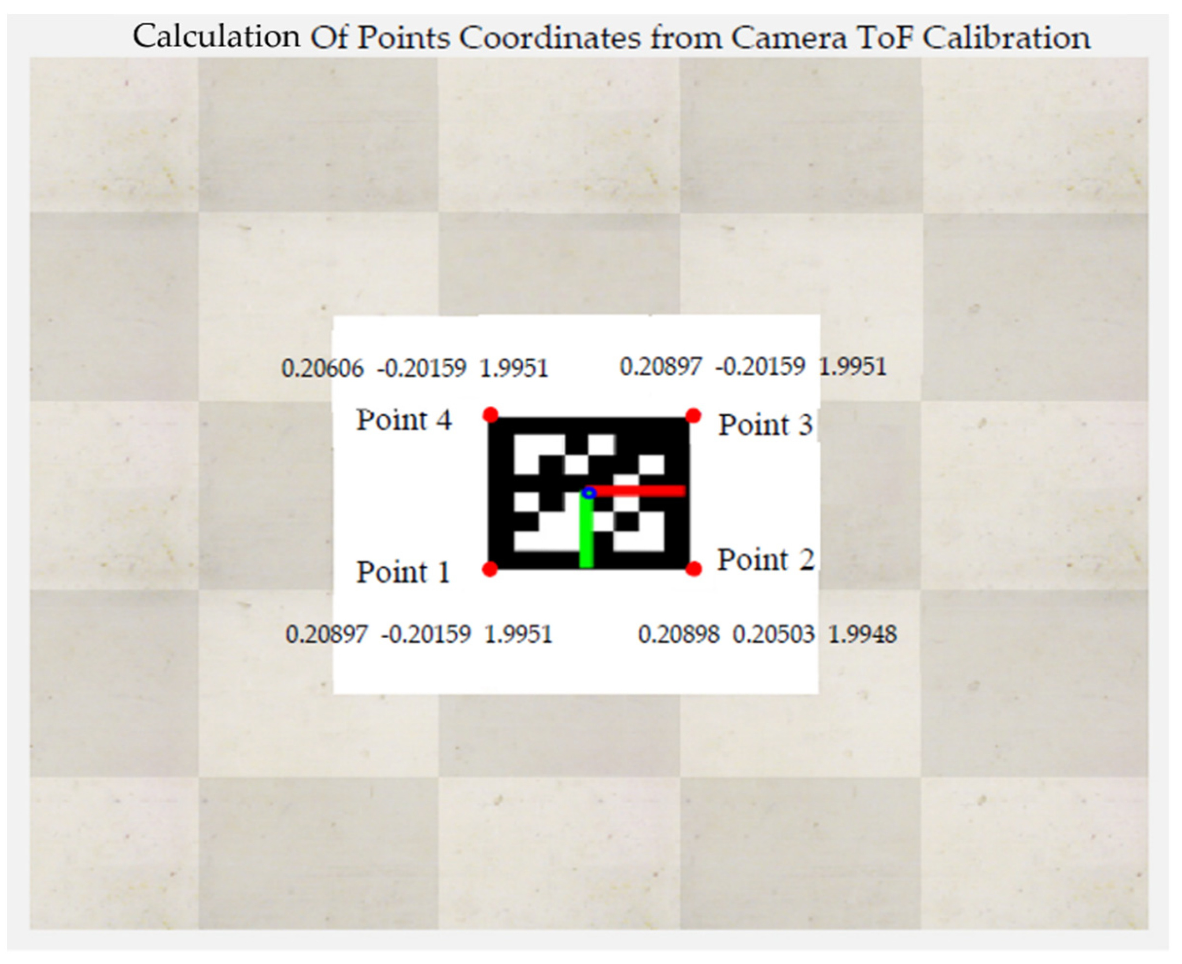
2.3. Camera ToF Calibration Implementation and Results
- Curve fitting with the hyperbola parametric mode as “f(x) = a/x + c” and then finding a and c parameters; and
- Interpolating between the found points.
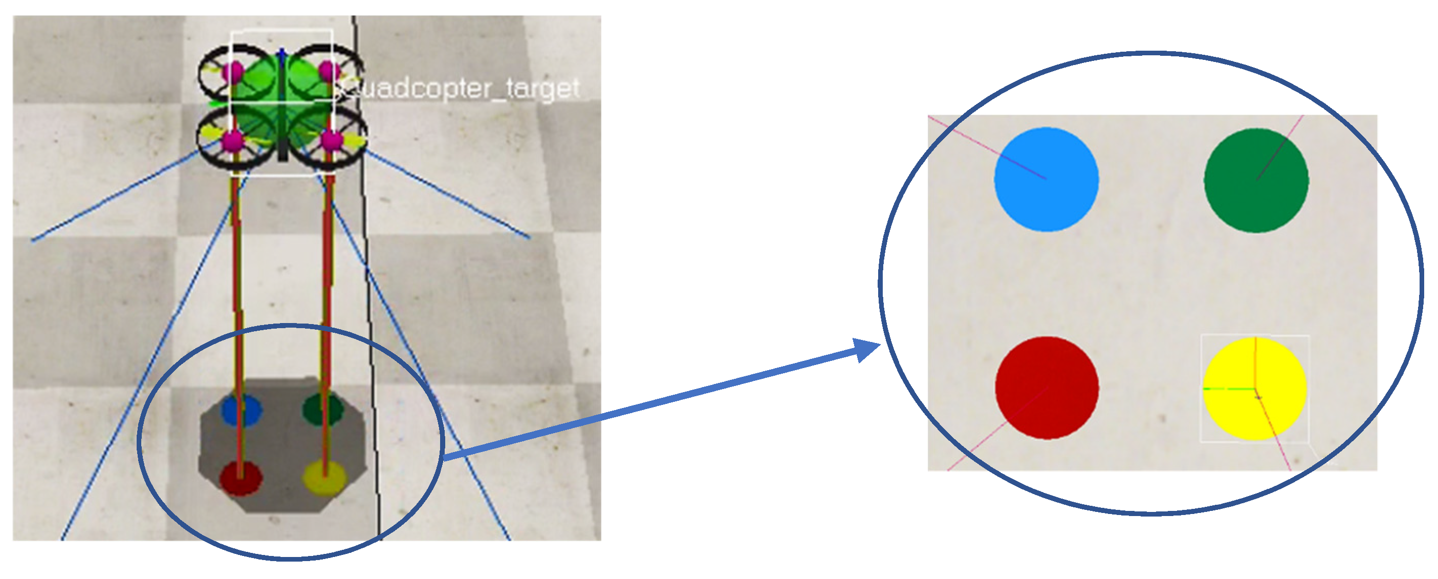
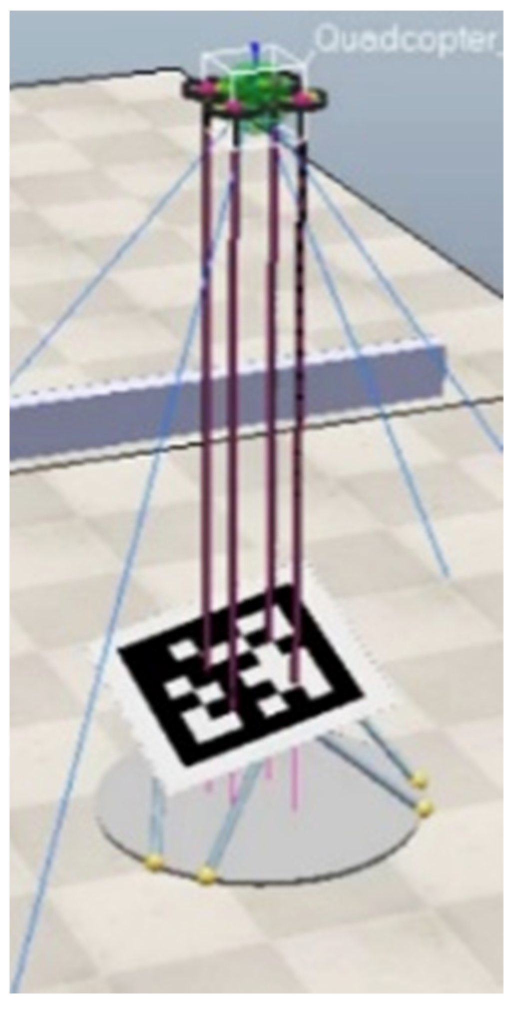
2.4. Calculation of the Planar Equation of the Landing Platform Beneath the Drone
2.5. AprilTag Corner Detection
- Detect the line segments;
- Quad detection;
- Homography and extrinsic estimation; and
- Payload decoding.
2.6. Kalman Filter Implementation
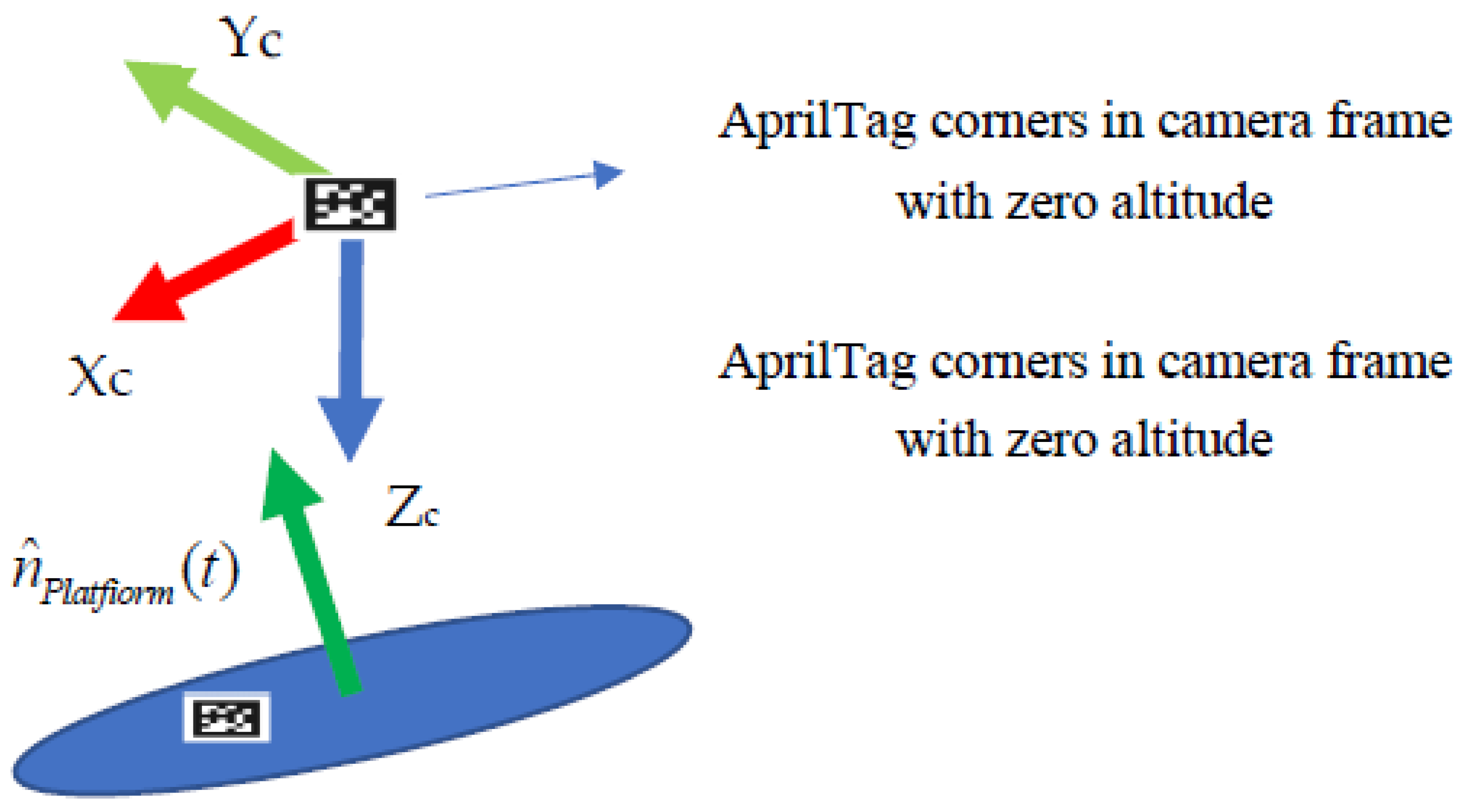
2.7. Landmark World Coordinates Calculation
2.8. Rigid Body Transformation Estimation of the AprilTag
3. Experimental Setups
4. Results and Discussion
4.1. Static Platform
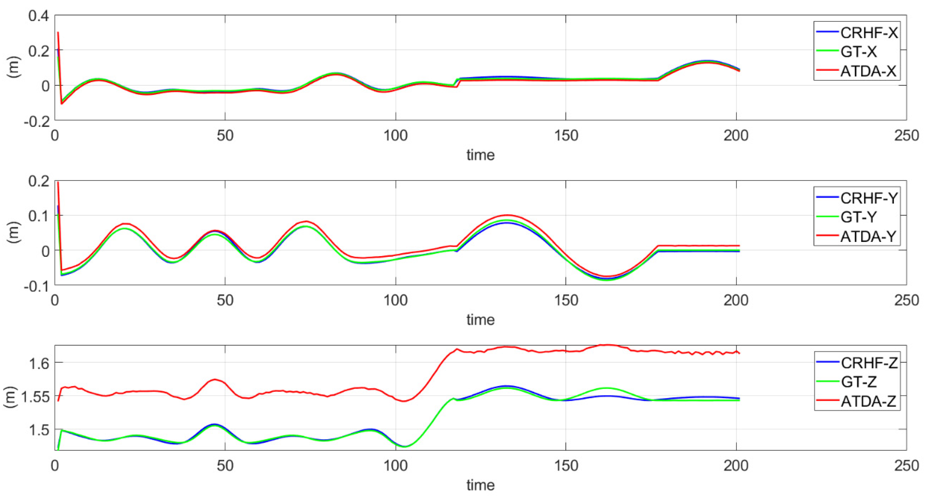
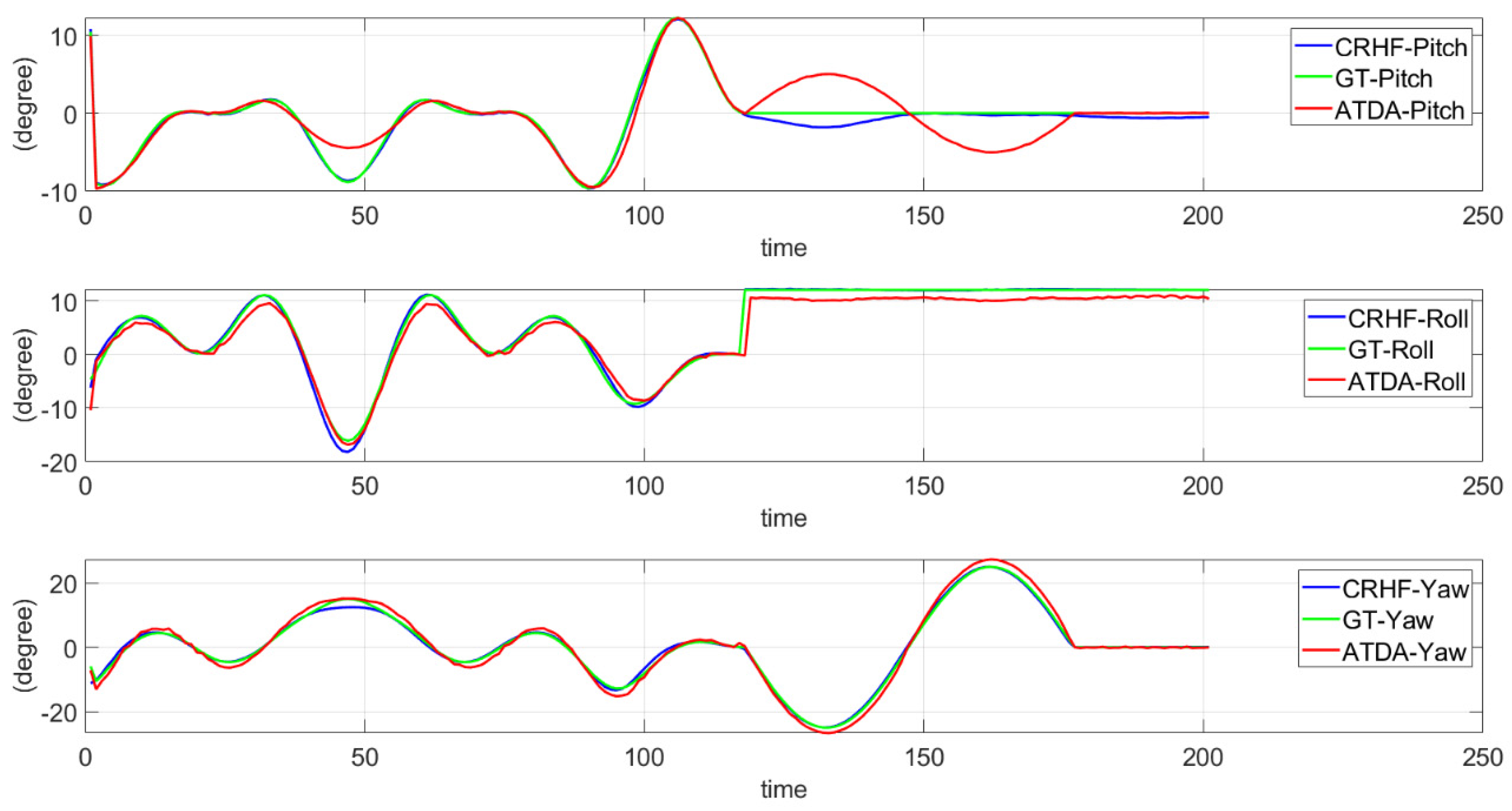
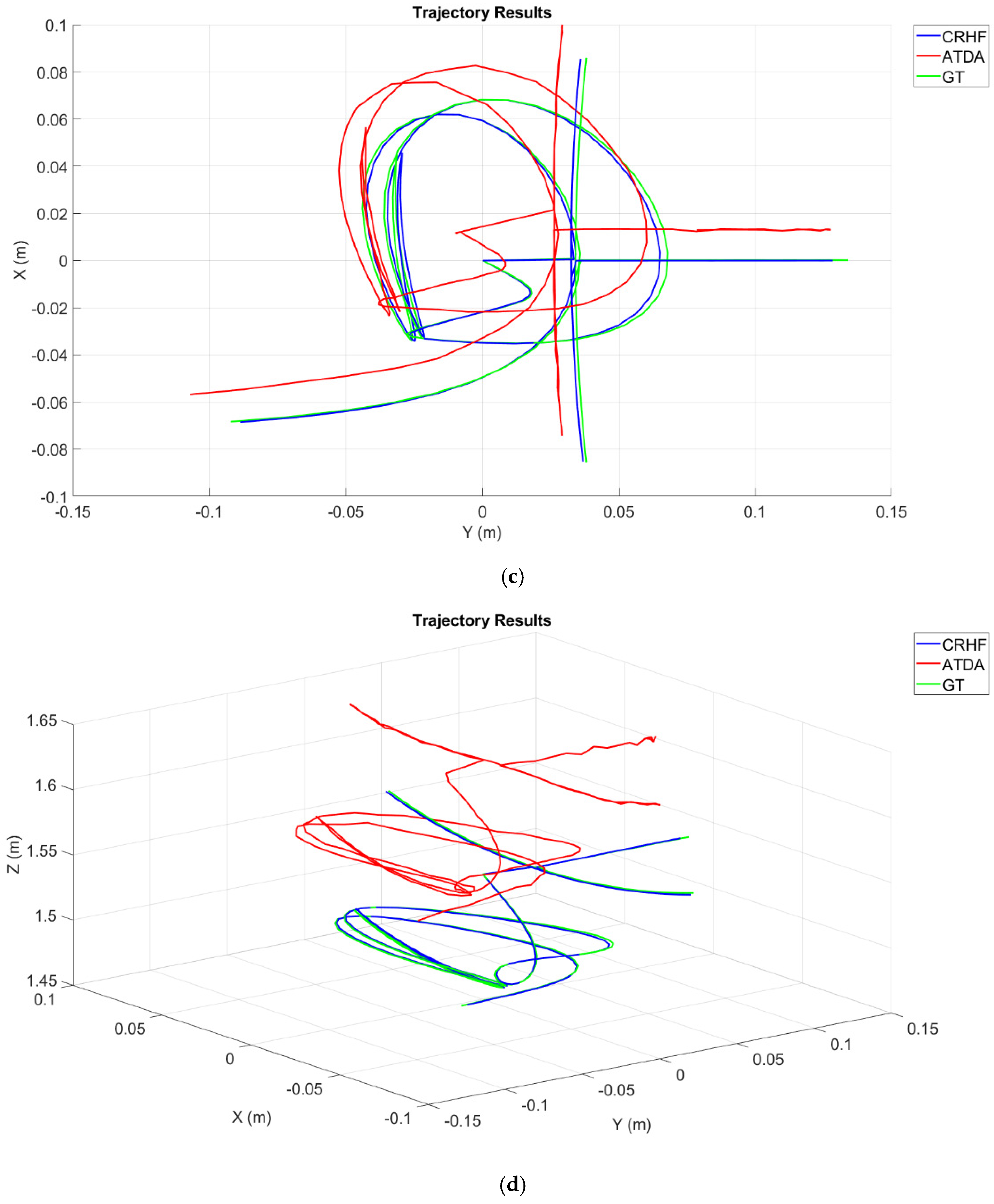
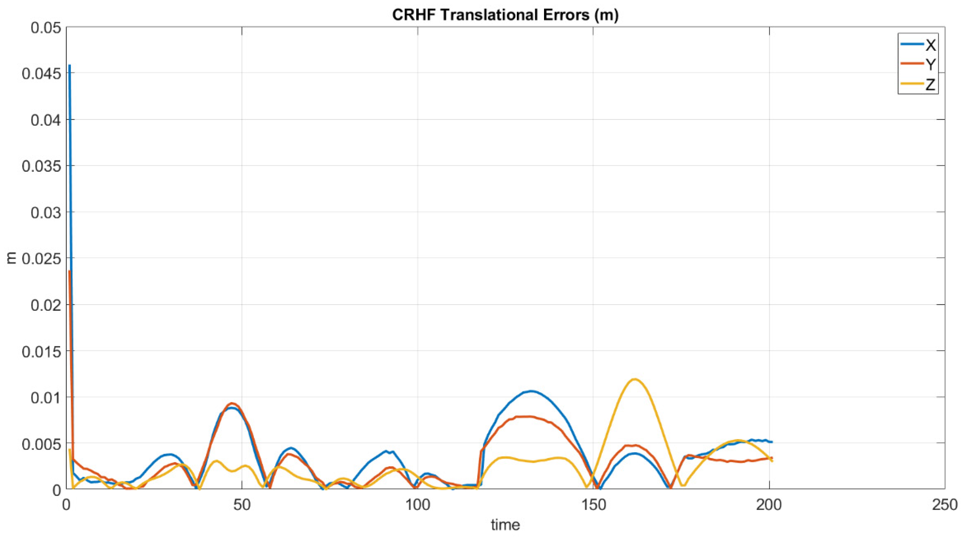
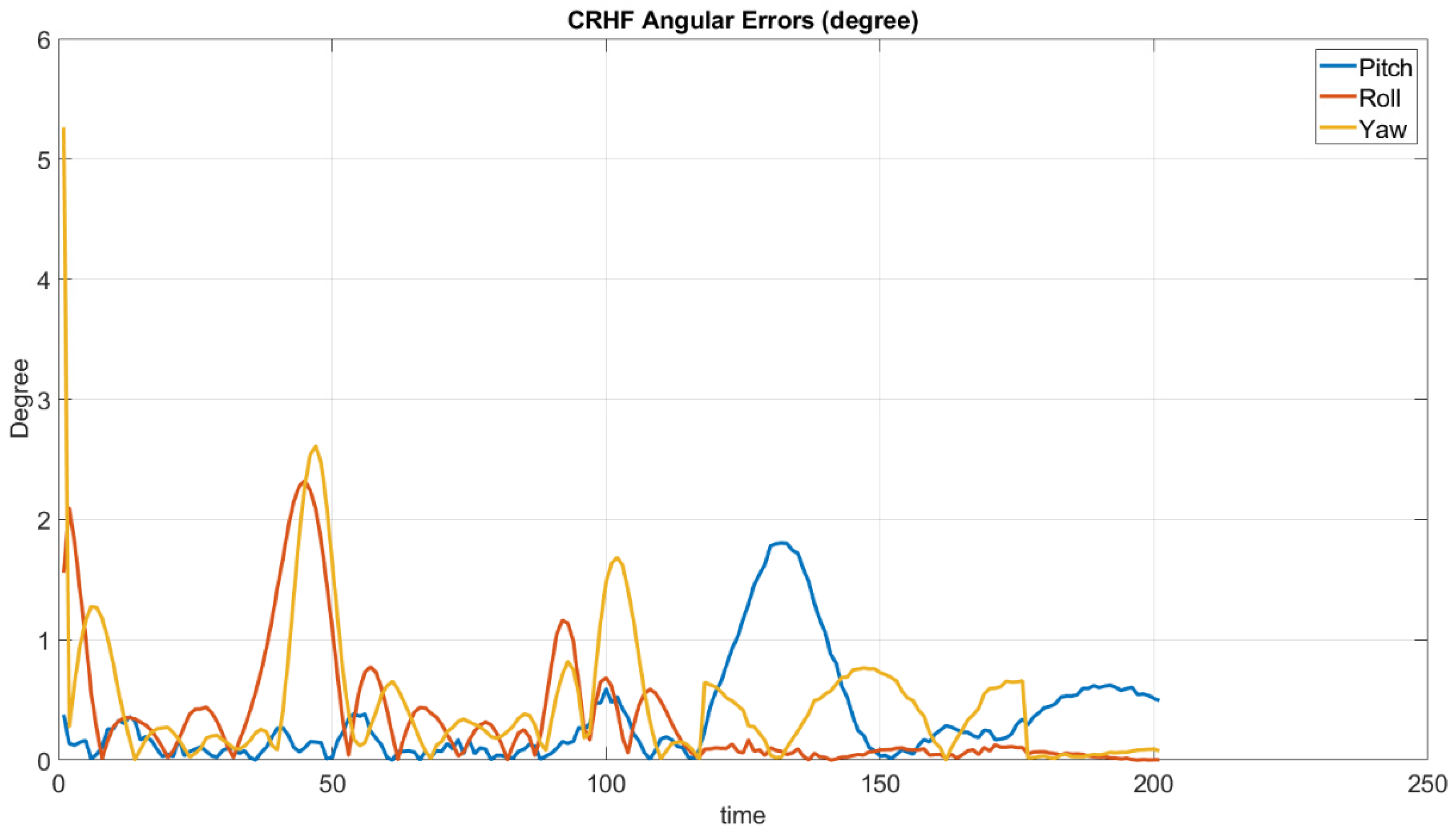
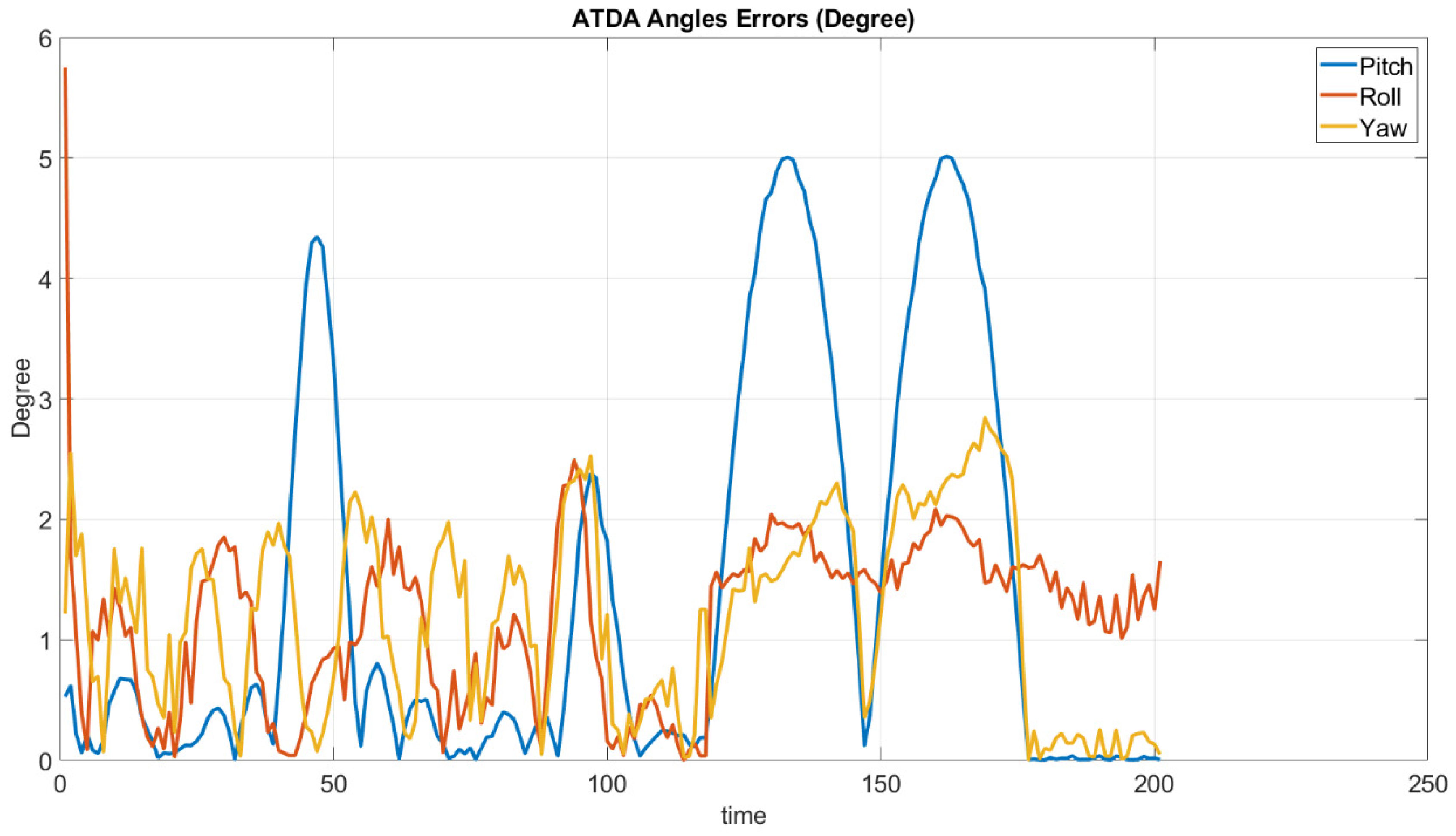
4.2. Dynamic Platform
5. Conclusions and Future Work
Author Contributions
Funding
Institutional Review Board Statement
Informed Consent Statement
Data Availability Statement
Acknowledgments
Conflicts of Interest
References
- Wubben, J.; Fabra, F.; Calafate, C.T.; Krzeszowski, T.; Marquez-Barja, J.M.; Cano, J.-C.; Manzoni, P. Accurate Landing of Unmanned Aerial Vehicles Using Ground Pattern Recognition. Electronics 2019, 8, 1532. [Google Scholar] [CrossRef] [Green Version]
- Yang, T.; Li, P.; Zhang, H.; Li, J.; Li, Z. Monocular Vision SLAM-Based UAV Autonomous Landing in Emergencies and Unknown Environments. Electronics 2018, 7, 73. [Google Scholar] [CrossRef] [Green Version]
- Lin, S.; Jin, L.; Chen, Z. Real-Time Monocular Vision System for UAV Autonomous Landing in Outdoor Low-Illumination Environments. Sensors 2021, 21, 6226. [Google Scholar] [CrossRef] [PubMed]
- Lee, D.-K.; Nedelkov, F.; Akos, D.M. Assessment of Android Network Positioning as an Alternative Source of Navigation for Drone Operations. Drones 2022, 6, 35. [Google Scholar] [CrossRef]
- Shi, G.; Shi, X.; O’Connell, M.; Yu, R.; Azizzadenesheli, K.; Anandkumar, A.; Yue, Y.; Chung, S.-J. Neural Lander: Stable Drone Landing Control Using Learned Dynamics. In Proceedings of the 2019 International Conference on Robotics and Automation (ICRA), Montreal, QC, Canada, 20–24 May 2019. [Google Scholar]
- Nguyen, P.H.; Arsalan, M.; Koo, J.H.; Naqvi, R.A.; Truong, N.Q.; Park, K.R. LightDenseYOLO: A Fast and Accurate Marker Tracker for Autonomous UAV Landing by Visible Light Camera Sensor on Drone. Sensors 2018, 18, 1703. [Google Scholar] [CrossRef] [Green Version]
- Truong, N.Q.; Lee, Y.W.; Owais, M.; Nguyen, D.T.; Batchuluun, G.; Pham, T.D.; Park, K.R. SlimDeblurGAN-Based Motion Deblurring and Marker Detection for Autonomous Drone Landing. Sensors 2020, 20, 3918. [Google Scholar] [CrossRef] [PubMed]
- Hamanaka, M.; Nakano, F. Surface-Condition Detection System of Drone-Landing Space using Ultrasonic Waves and Deep Learning. In Proceedings of the 2020 International Conference on Unmanned Aircraft Systems (ICUAS), Athens, Greece, 1–4 September 2020. [Google Scholar]
- Castellano, G.; Castiello, C.; Mencar, C.; Vessio, G. Crowd Detection for Drone Safe Landing through Fully-Convolutional Neural Networks. In SOFSEM 2020: Theory and Practice of Computer Science; Springer: Cham, Switzerland, 2020; pp. 301–312. [Google Scholar]
- Jung, S.; Hwang, S.; Shin, H.; Shim, D.H. Perception, Guidance, and Navigation for Indoor Autonomous Drone Racing Using Deep Learning. IEEE Robot. Autom. Lett. 2018, 3, 2539–2544. [Google Scholar] [CrossRef]
- Chang, C.-C.; Tsai, J.; Lu, P.-C.; Lai, C.-A. Accuracy Improvement of Autonomous Straight Take-off, Flying Forward, and Landing of a Drone with Deep Reinforcement Learning. Int. J. Comput. Intell. Syst. 2020, 13, 914. [Google Scholar] [CrossRef]
- Polvara, R.; Patacchiola, M.; Sharma, S.; Wan, J.; Manning, A.; Sutton, R.; Cangelosi, A. Toward End-to-End Control for UAV Autonomous Landing via Deep Reinforcement Learning. In Proceedings of the 2018 International Conference on Unmanned Aircraft Systems (ICUAS), Dallas, TX, USA, 12–15 June 2018; pp. 115–123. [Google Scholar]
- Rodriguez-Ramos, A.; Sampedro, C.; Bavle, H.; de la Puente, P.; Campoy, P. A Deep Reinforcement Learning Strategy for UAV Autonomous Landing on a Moving Platform. J. Intell. Robot. Syst. 2019, 93, 351–366. [Google Scholar] [CrossRef]
- Song, Y.; Steinweg, M.; Kaufmann, E.; Scaramuzza, D. Autonomous Drone Racing with Deep Reinforcement Learning. In Proceedings of the 2021 IEEE/RSJ International Conference on Intelligent Robots and Systems (IROS), Prague, Czech Republic, 27 September–1 October 2021. [Google Scholar]
- Santos, N.P.; Lobo, V.; Bernardino, A. Two-stage 3D model-based UAV pose estimation: A comparison of methods for optimization. J. Field Robot. 2020, 37, 580–605. [Google Scholar] [CrossRef]
- Khalaf-Allah, M. Particle Filtering for Three-Dimensional TDoA-Based Positioning Using Four Anchor Nodes. Sensors 2020, 20, 4516. [Google Scholar] [CrossRef] [PubMed]
- Kim, J.; Kim, S. Autonomous-flight Drone Algorithm use Computer vision and GPS. IEMEK J. Embed. Syst. Appl. 2016, 11, 193–200. [Google Scholar] [CrossRef]
- Khithov, V.; Petrov, A.; Tishchenko, I.; Yakovlev, K. Toward Autonomous UAV Landing Based on Infrared Beacons and Particle Filtering. In Advances in Intelligent Systems and Computing; Springer: Cham, Switzerland, 2016; pp. 529–537. [Google Scholar]
- Fernandes, A.; Baptista, M.; Fernandes, L.; Chaves, P. Drone, Aircraft and Bird Identification in Video Images Using Object Tracking and Residual Neural Networks. In Proceedings of the 2019 11th International Conference on Electronics, Computers and Artificial Intelligence (ECAI), Pitesti, Romania, 27–29 June 2019; pp. 1–6. [Google Scholar]
- Miranda, V.R.; Rezende, A.; Rocha, T.L.; Azpúrua, H.; Pimenta, L.C.; Freitas, G.M. Autonomous Navigation System for a Delivery Drone. arXiv 2021, arXiv:2106.08878. [Google Scholar] [CrossRef]
- Benini, A.; Mancini, A.; Longhi, S. An IMU/UWB/Vision-based Extended Kalman Filter for Mini-UAV Localization in Indoor Environment using 802.15.4a Wireless Sensor Network. J. Intell. Robot. Syst. 2013, 70, 461–476. [Google Scholar] [CrossRef]
- St-Pierre, M.; Gingras, D. Comparison between the unscented kalman filter and the extended kalman filter for the position estimation module of an integrated navigation information system. In Proceedings of the IEEE Intelligent Vehicles Symposium, Parma, Italy, 14–17 June 2004. [Google Scholar] [CrossRef]
- Raja, G.; Suresh, S.; Anbalagan, S.; Ganapathisubramaniyan, A.; Kumar, N. PFIN: An Efficient Particle Filter-Based Indoor Navigation Framework for UAVs. IEEE Trans. Veh. Technol. 2021, 70, 4984–4992. [Google Scholar] [CrossRef]
- Kraus, K. Photogrammetry: Geometry from Images and Laser Scans; Walter De Gruyter: Berlin, Germany; New York, NY, USA, 2007. [Google Scholar]
- Gruen, A.; Huang, T.S. Calibration and Orientation of Cameras in Computer Vision; Springer: Berlin/Heidelberg, Germany, 2021; Available online: https://www.springer.com/gp/book/9783540652830 (accessed on 29 September 2021).
- Luhmann, T.; Robson, S.; Kyle, S.; Boehm, J. Close-Range Photogrammetry and 3D Imaging; De Gruyter: Berlin, Germany, 2019. [Google Scholar]
- El-Ashmawy, K. Using Direct Linear Transformation (DLT) Method for Aerial Photogrammetry Applications. ResearchGate, 16 October 2018. Available online: https://www.researchgate.net/publication/328351618_Using_direct_linear_transformation_DLT_method_for_aerial_photogrammetry_applications (accessed on 29 September 2021).
- Sarris, N.; Strintzis, M.G. 3D Modeling and Animation: Synthesis and Analysis Techniques for the Human Body; Irm Press: Hershey, PA, USA, 2005. [Google Scholar]
- Aati, S.; Avouac, J.-P. Optimization of Optical Image Geometric Modeling, Application to Topography Extraction and Topographic Change Measurements Using PlanetScope and SkySat Imagery. Remote Sens. 2020, 12, 3418. [Google Scholar] [CrossRef]
- Morales, L.P. Omnidirectional Multi-View Systems: Calibration, Features and 3D Information. Dialnet. 2011. Available online: https://dialnet.unirioja.es/servlet/dctes?info=link&codigo=101094&orden=1 (accessed on 29 September 2021).
- Panoramic Vision, Panoramic Vision—Sensors, Theory, and Applications|Ryad Benosman|Springer. 2021. Available online: https://www.springer.com/gp/book/9780387951119 (accessed on 29 September 2021).
- Omnidirectional Vision Systems. Omnidirectional Vision Systems—Calibration, Feature Extraction and 3D Information|Luis Puig|Springer. Springer.com. 2013. Available online: https://www.springer.com/gp/book/9781447149460 (accessed on 29 September 2021).
- Faugeras, O.D.; Luong, Q.; Papadopoulo, T. The Geometry of Multiple Images: The Laws That Govern the Formation of Multiple Images of a Scene and Some; MIT Press: Cambridge, MA, USA, 2001. [Google Scholar]
- Zhang, Z. A flexible new technique for camera calibration. IEEE Trans. Pattern Anal. Mach. Intell. 2000, 22, 1330–1334. [Google Scholar] [CrossRef] [Green Version]
- Heikkila, J.; Silven, O. A four-step camera calibration procedure with implicit image correction. In Proceedings of the IEEE Computer Society Conference on Computer Vision and Pattern Recognition, San Juan, PR, USA, 17–19 June 1997; pp. 1106–1112. [Google Scholar]
- Learning OpenCV. Learning OpenCV; O’Reilly Online Learning; O’Reilly Media, Inc.: Sebastopol, CA, USA, 2021. [Google Scholar]
- Wang, J.; Shi, F.; Zhang, J.; Liu, Y. A new calibration model of camera lens distortion. Pattern Recognit. 2008, 41, 607–615. [Google Scholar] [CrossRef]
- Poynton, C. Digital Video and HD: Algorithms and Interfaces; Morgan Kaufmann: Amsterdam, The Netherlands, 2012. [Google Scholar]
- MathWorks, Inc. Image Processing Toolbox: User’s Guide; MathWorks, Inc.: Natick, MA, USA, 2016. [Google Scholar]
- Lens Calibration (Using Chessboard Pattern) in Metashape. 2021. Retrieved 27 January 2022. Available online: https://agisoft.freshdesk.com/support/solutions/articles/31000160059-lens-calibration-using-chessboard-pattern-in-metashape (accessed on 29 September 2021).
- Liang, Y. Salient Object Detection with Convex Hull Overlap. arXiv 2016, arXiv:1612.03284. [Google Scholar]
- Lin, S.; Garratt, M.A.; Lambert, A.J. Monocular vision-based real-time target recognition and tracking for autonomously landing an UAV in a cluttered shipboard environment. Auton. Robot. 2017, 41, 881–901. [Google Scholar] [CrossRef]
- Yadav, A.; Yadav, P. Digital Image Processing; University Science Press: New Delhi, India, 2021. [Google Scholar]
- Arthur, D.; Vassilvitskii, S. K-means++: The Advantages of Careful Seeding. Available online: http://ilpubs.stanford.edu:8090/778/1/2006-13.pdf (accessed on 29 September 2021).
- Corke, P. Robotics, Vision and Control—Fundamental Algorithms In MATLAB®, 2nd ed.; Springer: Berlin, Germany, 2017. [Google Scholar]
- Fritsch, F.N.; Butland, J. A Method for Constructing Local Monotone Piecewise Cubic Interpolants. SIAM J. Sci. Stat. Comput. 1984, 5, 300–304. [Google Scholar] [CrossRef] [Green Version]
- Moler, C.B. Numerical Computing with MATLAB; Society for Industrial and Applied Mathematics: Philadelphia, PA, USA, 2004. [Google Scholar]
- Olson, E. AprilTag: A robust and flexible visual fiducial system. In Proceedings of the 2011 IEEE International Conference on Robotics and Automation, Shanghai, China, 9–13 May 2011; pp. 3400–3407. [Google Scholar]
- Welch, G.; Bishop, G. An Introduction to the Kalman Filter; TR 95—041; University of North Carolina at Chapel Hill, Department of Computer Science: Chapel Hill, NC, USA, 1995. [Google Scholar]
- Blackman, S.S. Multiple-Target Tracking with Radar Applications; Artech House, Inc.: Norwood, MA, USA, 1986; p. 93. [Google Scholar]
- Arun, K.S.; Huang, T.S.; Blostein, S.D. Least-Squares Fitting of Two 3-D Point Sets. IEEE Trans. Pattern Anal. Mach. Intell. 1987, 9, 698–700. [Google Scholar] [CrossRef] [PubMed] [Green Version]


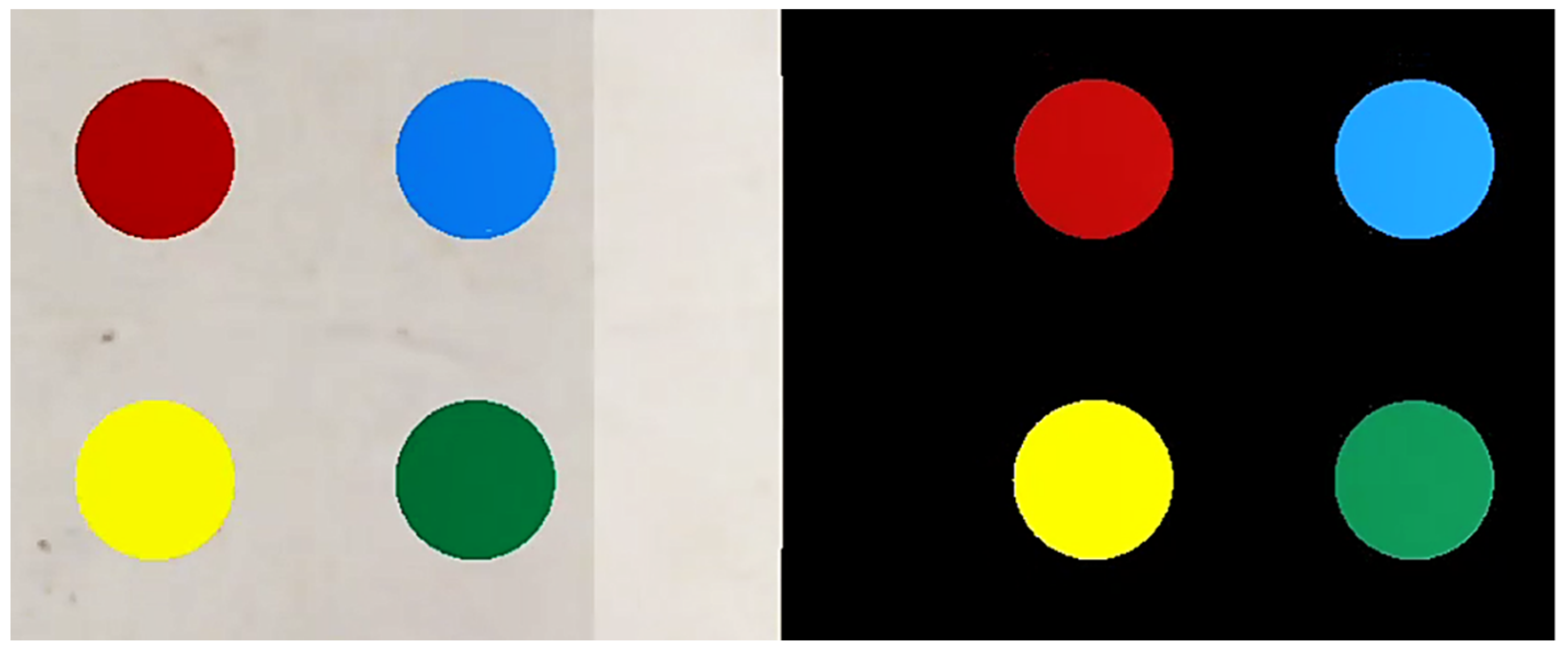
| Color | Channel 1 | Channel 2 | Channel 3 |
|---|---|---|---|
| Yellow | 103 < Range1 < 255 | 0 < Range2 < 95 | 0 < Range3 < 255 |
| Red | 0 < Range1 < 160 | 0 < Range2 < 255 | 167 < Range3 < 255 |
| Green | 0 < Range1 < 255 | 0 < Range2 < 155 | 0 < Range3 < 90 |
| Blue | 0 < Range1 < 165 | 139 < Range2 < 255 | 0 < Range3 < 255 |
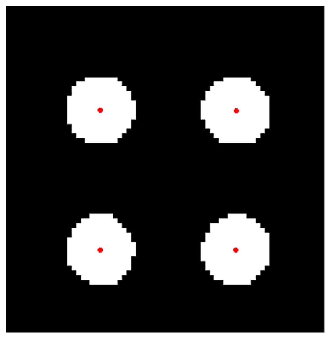
| Color | C1—Frame1 | C2—Frame2 | C3—Frame3 | |||
|---|---|---|---|---|---|---|
| Blue | 400.0070961 | 112.909046 | 392.6057903 | 120.4082739 | 383.8957617 | 129.1591336 |
| Green | 399.5563178 | 399.9410627 | 392.0877826 | 392.3846207 | 383.3468678 | 383.720831 |
| Yellow | 112.5299193 | 400.1530166 | 119.9678525 | 392.630475 | 128.6982725 | 384.0305636 |
| Red | 112.8321163 | 112.9362624 | 120.3259779 | 120.4101189 | 129.0014117 | 129.1613991 |
| Color | C1—Distance Frame1 | C2—Distance Frame2 | C3—Distance Frame3 |
|---|---|---|---|
| Blue | 0.305179805 | 0.32637015 | 0.348936737 |
| Green | 0.304939508 | 0.32626918 | 0.34884578 |
| Yellow | 0.304848552 | 0.32633689 | 0.348892212 |
| Red | 0.304876596 | 0.326466531 | 0.349034697 |
| Coordinate | X Coordinate | Y Coordinate | |
|---|---|---|---|
| Parameters | |||
| Coefficient trustworthiness | 95% confidence | 95% confidence | |
| Coefficient value | a = −44.43 | a = 44.43 | |
| c = 256.6 | c = 256.6 | ||
| Goodness of fit | SSE: 0.1409 | SSE: 0.1323 | |
| R-square: 1 | R-square: 1 | ||
| Adj-R-square: 1 | Adj-R-square: 1 | ||
| RMSE: 0.03456 | RMSE: 0.03348 | ||
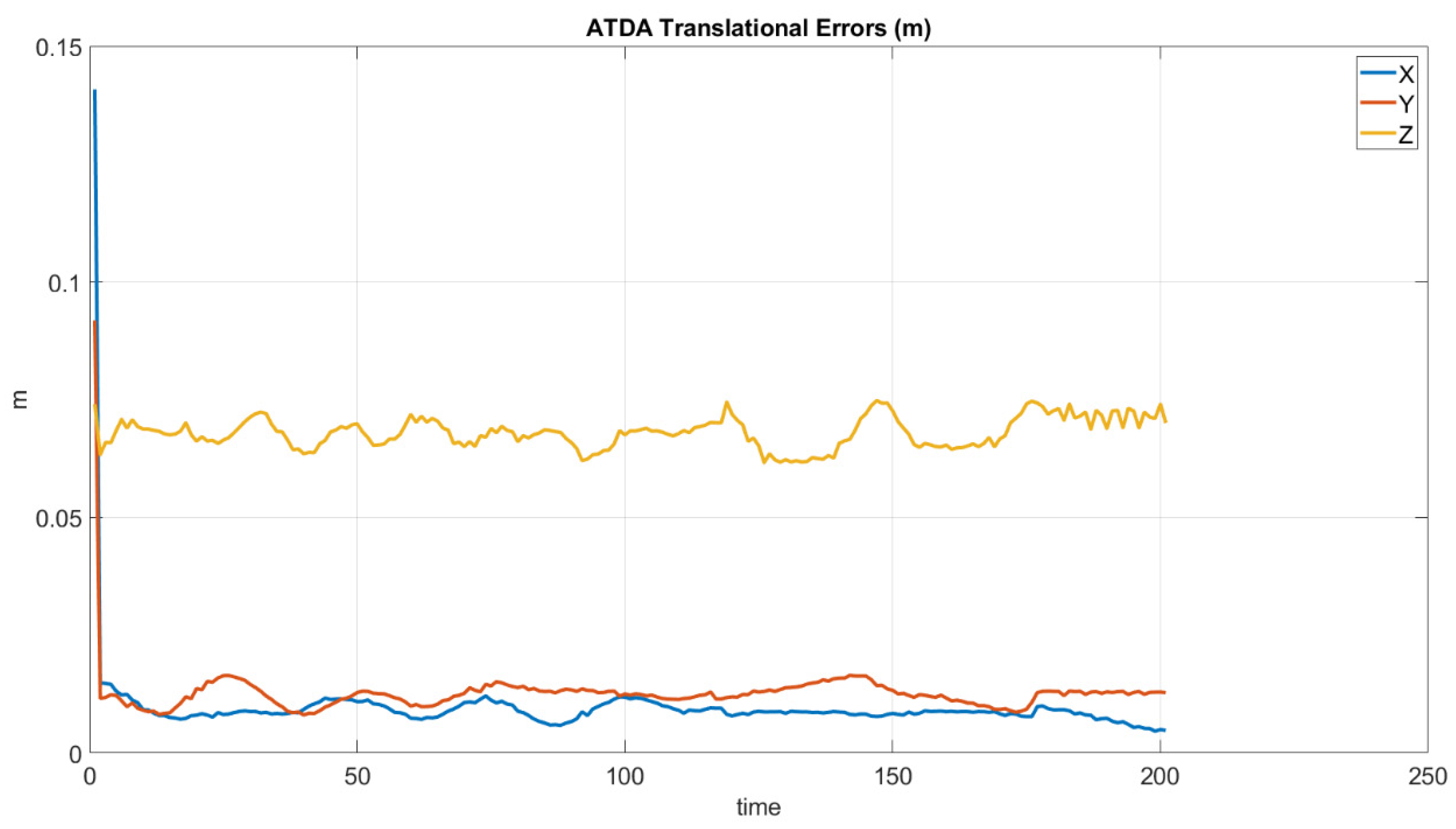
| Mean Absolute Error | ATDA | CRHF | ||||
|---|---|---|---|---|---|---|
| Translations (meters) | 0.0157 | 0.0129 | 0.0687 | 0.0047 | 0.0042 | 0.0051 |
| Angles (degrees) | 3.9043 | 1.7684 | 1.7859 | 1.4239 | 1.5231 | 1.3290 |
Publisher’s Note: MDPI stays neutral with regard to jurisdictional claims in published maps and institutional affiliations. |
© 2022 by the authors. Licensee MDPI, Basel, Switzerland. This article is an open access article distributed under the terms and conditions of the Creative Commons Attribution (CC BY) license (https://creativecommons.org/licenses/by/4.0/).
Share and Cite
Sefidgar, M.; Landry, R., Jr. Unstable Landing Platform Pose Estimation Based on Camera and Range Sensor Homogeneous Fusion (CRHF). Drones 2022, 6, 60. https://doi.org/10.3390/drones6030060
Sefidgar M, Landry R Jr. Unstable Landing Platform Pose Estimation Based on Camera and Range Sensor Homogeneous Fusion (CRHF). Drones. 2022; 6(3):60. https://doi.org/10.3390/drones6030060
Chicago/Turabian StyleSefidgar, Mohammad, and Rene Landry, Jr. 2022. "Unstable Landing Platform Pose Estimation Based on Camera and Range Sensor Homogeneous Fusion (CRHF)" Drones 6, no. 3: 60. https://doi.org/10.3390/drones6030060
APA StyleSefidgar, M., & Landry, R., Jr. (2022). Unstable Landing Platform Pose Estimation Based on Camera and Range Sensor Homogeneous Fusion (CRHF). Drones, 6(3), 60. https://doi.org/10.3390/drones6030060