Article

Accuracy Assessment of a UAV Direct Georeferencing Method and Impact of the Configuration of Ground Control Points

1
School of Mining Engineering, Taiyuan University of Technology, Taiyuan 030024, China
2
Shanxi Provincial Key Lab of Resources, Environment and Disaster Monitoring, Shanxi Coal Geology Geophysical Surveying Exploration Institute, Jinzhong 030600, China
*
Author to whom correspondence should be addressed.
Drones 2022, 6(2), 30; https://doi.org/10.3390/drones6020030
Submission received: 2 January 2022 / Revised: 16 January 2022 / Accepted: 17 January 2022 / Published: 20 January 2022
(This article belongs to the Special Issue Unconventional Drone-Based Surveying)

Abstract

:
Unmanned aerial vehicles (UAVs) can obtain high-resolution topography data flexibly and efficiently at low cost. However, the georeferencing process involves the use of ground control points (GCPs), which limits time and cost effectiveness. Direct georeferencing, using onboard positioning sensors, can significantly improve work efficiency. The purpose of this study was to evaluate the accuracy of the Global Navigation Satellite System (GNSS)-assisted UAV direct georeferencing method and the influence of the number and distribution of GCPs. A FEIMA D2000 UAV was used to collect data, and several photogrammetric projects were established. Among them, the number and distribution of GCPs used in the bundle adjustment (BA) process were varied. Two parameters were considered when evaluating the different projects: the ground-measured checkpoints (CPs) root mean square error (RMSE) and the Multiscale Model to Model Cloud Comparison (M3C2) distance. The results show that the vertical and horizontal RMSE of the direct georeferencing were 0.087 and 0.041 m, respectively. As the number of GCPs increased, the RMSE gradually decreased until a specific GCP density was reached. GCPs should be uniformly distributed in the study area and contain at least one GCP near the center of the domain. Additionally, as the distance to the nearest GCP increased, the local accuracy of the DSM decreased. In general, UAV direct georeferencing has an acceptable positional accuracy level.

1. Introduction

As a new aerial survey platform, unmanned aerial vehicles (UAVs) have attracted increasing attention worldwide. Compared with methods based on satellite or airborne sensors, UAVs provide user-defined spatial and temporal resolution data at a relatively low cost, as well as flexible options for sensor use and data collection [1]. Images captured by UAVs and processed by structure-from-motion (SfM) photogrammetry are a combination of mature photogrammetry principles and modern computer vision technology [2] (hereafter UAV SfM). UAV SfM is widely used in Earth and Environmental Sciences to generate high-resolution topography (HRT) data [3,4], including precision agriculture [5,6], landslide monitoring [7,8], coastal change [9,10], and glacier dynamics [11,12].
Georeferencing is the process of referencing the results of bundle adjustment (BA) and photogrammetric processes to a specific coordinate system [13]. During bundle adjustment (BA), ground control point (GCP) coordinates on the ground are provided and measured in the images (indirect georeferencing) or known external elements of the images are directly used (direct georeferencing) [14]. Direct georeferencing requires cm-level positioning accuracy of the UAV, obtained by difference data. GCP field deployment, surveying, and recognition in images may require a significant amount of time and cost, while direct georeferencing based on IMU and GNSS can quickly collect data and significantly improve work efficiency. However, these benefits are only valuable if the accuracy of the directly georeferenced topographic product meets the requirements of the application. First, the GNSS mobile receiver on the UAV achieves centimeter-level positioning accuracy by receiving difference data provided by a virtual reference station (VRS), and then adds the position data solved by the fusion of real-time kinematic (RTK) and post-processed kinematic (PPK) into the BA process. Direct georeferencing requires obtaining the coordinates of a GNSS receiver at the exact moment the image is acquired, although RTK can provide high-accuracy single-point positioning. However, there might be distortions in signals from satellite constellations and interruptions in RTK connections for a fast-flying UAV. Fusion PPK technology can solve epoch data in the lockout period through a reverse Kalman filter to improve the fixed rate and positioning accuracy [15,16].
Considering the rapid development of UAV technology, it is necessary to evaluate the accuracy of UAV direct georeferencing methods with GNSS RTK/PPK technology. Many studies have evaluated the technology based on measured checkpoints on the ground. Padró et al. evaluated the data of a farm and showed that the horizontal and vertical RMSE of direct georeferencing were no more than 0.256 and 0.238 m, respectively [17]. Nolan et al. obtained data with a GSD of 10–20 cm in an area over tens of square kilometers and verified that the accuracy and precision (repeatability) of direct georeferencing were better than ±30 and ±8 cm, respectively, at 95% RMSE [18]. In the other two studies, the vertical RMSE did not exceed 10 and 20 cm, respectively [19,20]. The accuracy of the vertical direction is not always able to meet the requirements, and the accuracy can only reach the meter level in some studies [21,22]. Mian obtained a vertical RMSE of 40 cm using an image of 0.7 cm GSD [23]. Hugenholtz compared direct and indirect georeferencing methods, and recommended using GCPs where high accuracy is required [24].
The final product quality mainly depends on camera specifications, GCP configuration (accuracy, density and distribution), flight parameters (image overlap, GSD, etc.), land cover and terrain complexity, processing software, and flight platform (fixed wing or rotor wing). Measuring GCP is a time-consuming task, so a balance between appropriate accuracy and efficiency is needed. The literature to date shows consistently that accuracy increased with an increase in the number of GCPs and rapidly reached an asymptotic trend [25,26,27]. Conclusions differ among studies regarding the amount of GCPs required to produce a favorable outcome. In [28], 0.5~1 GCP per ha was the optimal GCP density, and GCPs were placed inside the area with stratified distribution to obtain the minimum total error. In [29], the optimal density was 1.8 GCPs per ha, uniformly distributed across the whole surface. Scott et al. reported setting control points in the center and edge of the study area, which is of great significance to reduce the height vertical error in spatial concentration [30].
The purpose of this study was to evaluate the accuracy of UAV RTK/PPK direct georeferencing and to determine whether the method could be used as a solution for rapid mapping applications with data generated from images of natural environments, including buildings, low vegetation and so on. The aim was to understand the difference in survey effectiveness between using direct georeferencing and GCPs. In addition, the effect of GCP quantity and distribution on the quality of the results was also studied. The evaluation was performed by calculating the vertical and horizontal RMSE of checkpoints on a digital surface model (DSM) and digital orthomosaic (DOM), respectively, and the Multiscale Model to Model Cloud Comparison (M3C2) distance based on point clouds [31]. The M3C2 method is the unique way to compute signed (and robust) distances directly between two point clouds.

2. Materials and Methods
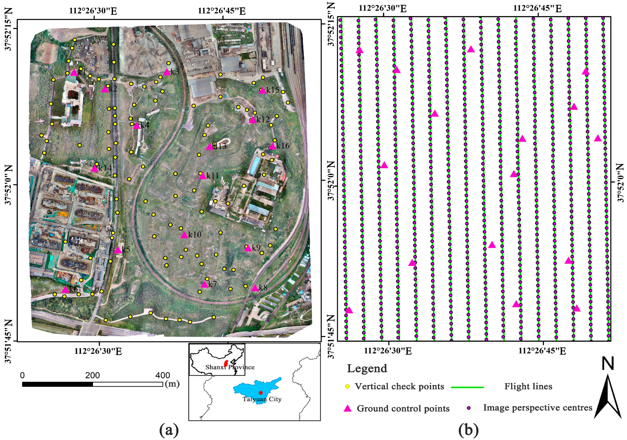
The workflow of this study is shown in Figure 1. The study comprises four main steps: route planning (field survey, pre-flight, and setting flight parameters); data acquisition (ground GCP and CP layout and survey, UAV image acquisition); data processing considering different quantities of GCPs (BA and image-intensive matching); and horizontal and vertical quality assessment (data and error analysis).

2.1. The Study Area

The study area is located near Xishan, Taiyuan, Shanxi Province, People’s Republic of China (Figure 2). The approximate coordinates in the geodetic reference system WGS84 are 112°27′5.64″ E and 37°52′0.98″ N. The region covers an area of approximately 0.5 km2, with the highest point at 896 m and the lowest point at 840 m. The area features railways, factories, and low vegetation.
Accurate GCP coordinates are required for georeferencing UAV images. Sixteen ground survey markers were deployed, according to different photogrammetric projects—some of them were used as the input of the BA process, and the rest were used as horizontal checkpoints for cross verification of the horizontal accuracy. All control points were as evenly distributed as possible in the study area. In addition, coordinates of 120 points were obtained for vertical accuracy analysis of the generated DSM. Compared to CPs for horizontal accuracy assessment, vertical CPs do not require accurate identification in the image. Aerial markers consisted of 70 × 70 cm highly reflective red and yellow material fixed with nails to the ground, far away from high vegetation, buildings, and slopes. These markers were large enough to be identified in images and placed and measured prior to flight. A GNSS RTK receiver was used for field measurements. The receiver was connected to a virtual reference station and received differential signals through the network. Ten fixed solutions were recorded at each point, and the average was taken as the final result. Taking the average of the results of multiple measurements as the final result can exclude the influence of accidental factors and make the measurement results closer to the true value. At a control point marker, it takes about 3–5 min from deployment to the end of measurement. All coordinates were recorded in the WGS84 reference system. In the experiment, the means of the RTK coordinate residuals in the X, Y, and Z directions were 0.007, 0.006, and 0.012 m, respectively. The expected coordinate accuracy was higher than the spatial resolution of the UAV image (GSD about 1.7 cm). Figure 2 shows the position of GCPs and CPs relative to the study area.

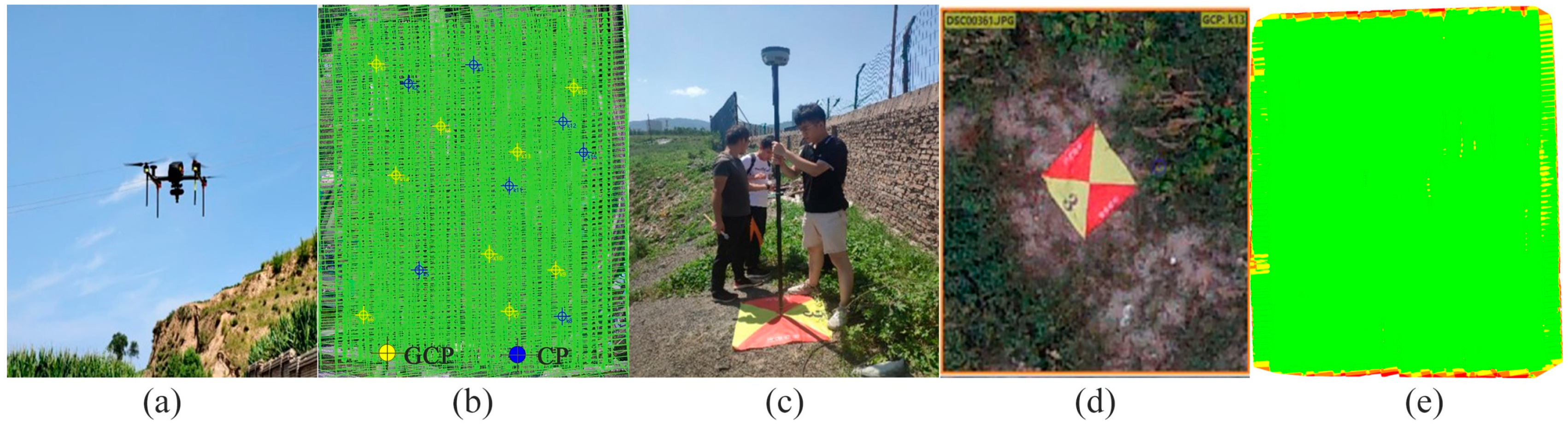
2.2. Data Collection

In this study, a FEIMA D2000 multi-rotor UAV (Figure 3a) was used to collect data. This UAV included a fuselage, power motor, quick removal wing, differential antenna, magnetometer, and data transmission antenna. The 24.3-megapixel camera installed on the D2000 UAV provided a ground sampling distance (GSD) of 1.7 cm/pixel at an altitude of 110 m relative to the ground. The camera captured images at fixed intervals and stored them in JPG format. Detailed information about the UAV and camera are shown in Table 1.
By pre-setting flight parameters in the UAV Manager software, the UAV flew autonomously from takeoff to landing. The ground control station consisted of computers, a ground-based data transmission radio, and antennas that communicated with the UAV to continuously monitor its flight status and allowed users to interrupt the flight if the UAV was in danger. The aerial survey was conducted on 10 August 2021 with clear weather and light wind.

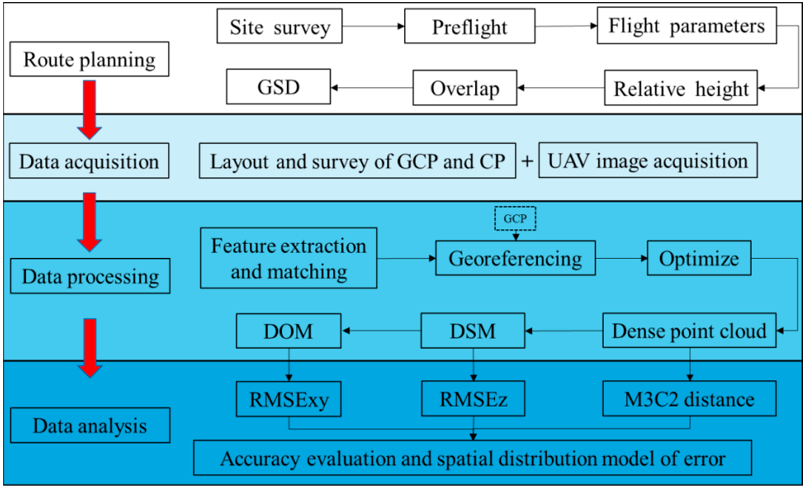
2.3. Data Processing

In this study, Agisoft Photoscan Professional Version 1.7.0 [32] software was used to generate dense point clouds, a DSM, and a DOM based on the SfM algorithm. Before processing, position data were solved by the network RTK/PPK fusion differential job mode, which gave priority to the results of the PPK fixed solution, while for the non-fixed solution part of PPK, RTK fixed solution data were used for fusion, so as to ensure the quality of high-precision position data through complementary operation mode, and the RTK trajectory file was input during fusion difference resolution. Then, image EXIF was sequentially written—that is, the GPS positioning data were stored in the header file of the image, so that the GPS data could be directly read through the image in the software. The workflow in Photoscan is described as follows:
  • Image feature extraction and matching. The software automatically identifies many conspicuous points in each image, regardless of image scale or perspective, and similar feature points are recognized in multiple images. After locating the feature points in each image, similar feature points are recognized in multiple images. The quality of feature matching depends on the texture and overlap success of the image [33,34];
  • Iterative bundle adjustment. The purpose of BA is to determine internal and external orientation elements of the images by minimizing the reprojection errors between predicted and observed points, which can be converted into a nonlinear least-squares problem [35]. By applying the BA, the three-dimensional structure of the scene, the internal and external orientation elements of the camera are estimated at the same time;
  • Model optimization based on control points. GCPs provide additional external information about reconstructed scene geometry. The optimization process in Photoscan refines the camera position and reduces non-linear project deformations by incorporating GCPs [36];
  • Point cloud density matching. The MVS image matching algorithm operates on a single-pixel scale of the image to build dense clouds and increases the point density by several orders of magnitude;
  • Generate DSM and DOM. Using the dense point cloud as input, other results, such as DSM and DOM, can be produced. The outliers in the dense point cloud are removed before the dense point cloud is interpolated to generate DSM, and then the DOM is generated by digital differential correction based on DSM.
The images in all projects underwent the same photogrammetric processing, with differences in the number and distribution of GCPs used in the BA process. The number of GCPs in the experiment for evaluating the vertical RMSE ranged from 0 to 16, while the number for the horizontal RMSE ranged from 0 to 10. Seven other experiments evaluated the impact of the GCP distribution; the distribution schemes are shown in Figure 4.

2.4. Quality Assessment

Two methods were used to evaluate the quality of the UAV SfM results. The first method evaluates the accuracy of the DSM and DOM generated by different projects. The root mean square error (RMSE) was further calculated by comparing the CP coordinates estimated in the calculation results with the reference CP coordinates measured with the GNSS RTK receiver. Specifically, horizontal accuracy was verified on DOM, while vertical accuracy was verified by extracting the elevation of the corresponding DSM on a larger range of 120 vertical checkpoints.
R M S E X = i = 1 n Δ x i 2 n ,
R M S E Y = i = 1 n Δ y i 2 n ,
R M S E Z = i = 1 n Δ z i 2 n ,
where Δ x , Δ y , and Δ z are the differences between RTK checkpoint coordinates and model-extracted coordinates, and n is the number of checkpoints. Calculation of the horizontal RMSE ( R M S E XY ) is as follows:
R M S E X Y = R M S E X 2 + R M S E Y 2 ,
The second method uses the Multiscale Model to Model Cloud Comparison (M3C2) tool of the CloudCompare software version 2.10. [37], which calculates the distance of the reference cloud and comparison point cloud relative to the local surface normal direction through two parameters (user-defined normal proportion and projection proportion). The process runs directly on the point cloud and does not require grid partitioning, avoiding the uncertainties involved in the interpolation process.
To compare point clouds, the M3C2 distance between the reference point cloud generated by the 16 GCPs participating in BA and other project point clouds was calculated. Then, the mean and standard deviation of the M3C2 distance calculation were used to evaluate the accuracy and precision, respectively, of each point cloud. By plotting the error and its distribution curve, we determined the influence of the GCP distribution on the spatial distribution of the M3C2 distance difference and determined the possible pattern of the spatial distribution of error.

3. Results

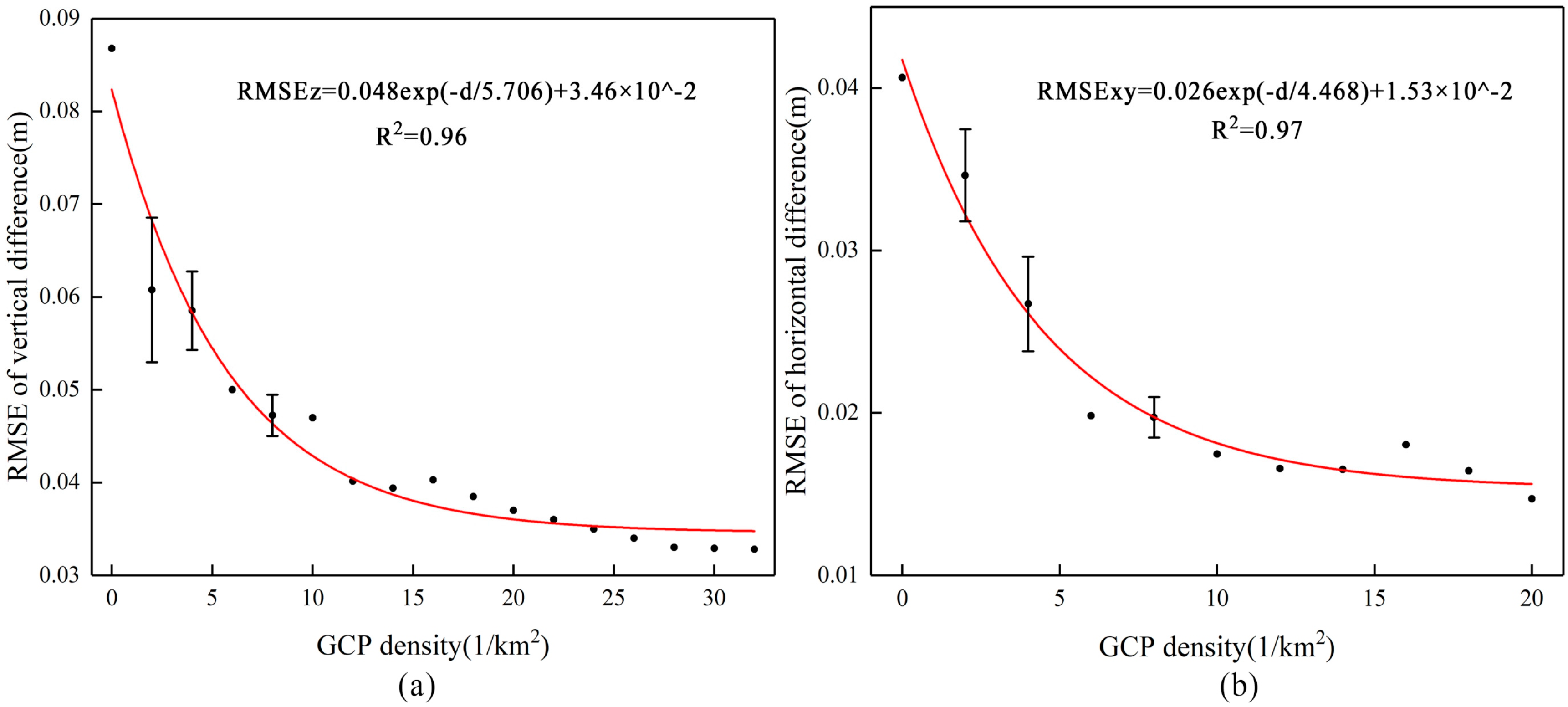
3.1. Model Evaluation Based on RMSE

Based on the model extraction coordinates and measured checkpoint coordinates, the vertical and horizontal RMSE for each project were calculated using Equations (1)–(4). The GCP density was calculated from the number of GCPs used divided by the area investigated; the relationship between GCP density and RMSE was obtained, as shown in Figure 5. The results show that when the GCP density was highest, the vertical and horizontal RMSE were 0.032 and 0.015 m, respectively, representing approximately 1.88 and 0.88 GSD. When GCPs were not used, the vertical and horizontal RMSE increased to 0.087 and 0.041 m, respectively, representing a GSD of approximately 5.12 and 2.41. R M S E XY was less than R M S E Z in all projects. The mean ratio of R M S E Z : R M S E XY is approximately 2.3. As the density of the GCP increased, the vertical and horizontal RMSE gradually decreased; this trend is fitted by the nonlinear curve in Figure 5. As shown in Figure 5a, when d > 12 GCP/km2, the vertical RMSE did not significantly decrease (the change from the maximum was less than 20%). In Figure 5b, the same is true for d > 10 GCP/km2 when considering the horizontal RMSE (the error does not show significant change).
There are some cases when the GCP density increased and the RMSE increased, which may be due to the error introduced by the ground measurement of the newly added GCPs. Our results for the horizontal error evaluation are influenced by manually setting the coordinates in the center of the GCPs. A similar uncertainty is expected when determining the coordinates of the GCP centers on the DOM.
Statistical analysis of the vertical differences of the three projects is shown in Figure 6. In Figure 6a–c, the histograms of the differences between RTK checkpoint elevations and DSM extraction elevations correspond to 0, 1, and 2 GCPs, respectively; all of the curves exhibit a Gaussian distribution. The mean value depicted in Figure 6a is −0.08 m, indicating a systematically biased distribution. The mean value in Figure 6b is −0.025 m, indicating that the addition of a single GCP is conducive to reducing the vertical error. When two GCPs are considered (Figure 6c), the mean value is 0.003 m, and the distribution is significantly improved. A single sample t-test was conducted, as shown in Table 2. The null hypothesis is that there is no significant difference between the mean and the test value 0. The significance of one GCP is less than 0.05, rejecting the original hypothesis, that is, there is a significant difference between the mean of one GCP and zero at a 95% confidence interval. The significance of two GCPs was 0.449, greater than 0.05, and the original hypothesis was accepted—that is, there was no significant difference between the mean of two GCPs and zero at a 95% confidence interval. Therefore, the DSM has systematic dome error in the vertical direction when zero or one GCP was used, and it is important to use at least two GCPs to improve DSM elevation accuracy. The standard deviation did not show a significant difference, with one GCP having the lowest standard deviation, at 0.033. Figure 6d shows the linear fit of the height difference between the DSM obtained by checkpoints and zero GCPs used; the coefficient of determination (R2) is 0.99.

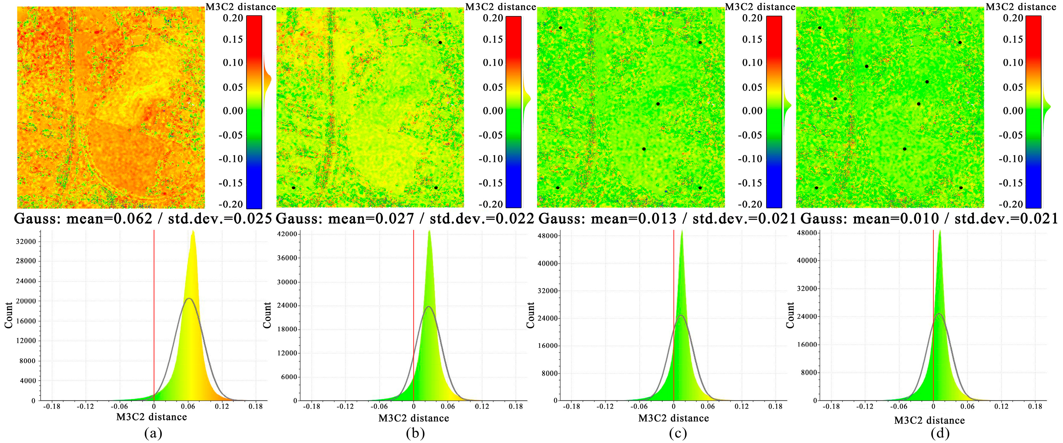
3.2. Point Cloud Evaluation Based on M3C2 Distance

The M3C2 distance between the reference point cloud (16 GCPs of the BA process) and point cloud obtained from different projects was calculated. Mean and standard deviation were used as indicators to evaluate the accuracy and precision, respectively, of the point clouds of different projects (Table 3 and Figure 7). The mean distance between point clouds obtained by zero GCPs and the reference point cloud was 0.062 m. Adding a GCP at any position can reduce the mean distance, and the improvement is most obvious after adding K8 GCP in the lower right corner. Regardless of the distribution, when using two GCPs, the mean error can be reduced by about 50% compared with 0 GCPs. With an increase in the number of GCPs, the mean distance decreased, and the point cloud became more accurate. The mean distance decreased to a minimum of 0.01 m at eight and nine GCPs. The standard deviations of different projects were distributed between 0.02 and 0.03, showing no obvious difference. Several projects achieved a minimum standard deviation of 0.021 m.
The error space distributions of the M3C2 distance between the reference point cloud and the point clouds of the 0-, 3-, 6-, and 9-GCP projects were calculated, and the results are displayed with the same legend and histogram distribution of the distance (Figure 8). A significant dome effect (red area) can be observed at zero GCPs in Figure 8a; the upper left corner of Figure 8b shows a clear error compared with the reference point cloud due to a lack of control; the error from Figure 8c to Figure 8d is not significantly reduced, which is only reflected in the mean distance (from 0.013 to 0.01 m).
Overall, the accuracy near the boundary of the study area is not as high as that in the center, which is related to the low overlap of images near the boundary (Figure 3e). There are obvious errors along the north–south road and the boundaries of buildings. The reasons for the large M3C2 distance error along the road are as follows: (1) tall plants on both sides of the road block the ground; (2) sample data from the road area are extracted, and the calculated point cloud density is approximately 12 per m2, which is less than the average density of approximately 35 per m2 in the overall study area. The uniform surface of the road (asphalt pavement) lacks adequate feature points, resulting in a sparse area within the point cloud. The M3C2 distance increased at the boundaries of buildings due to the sudden change in topographic characteristics.

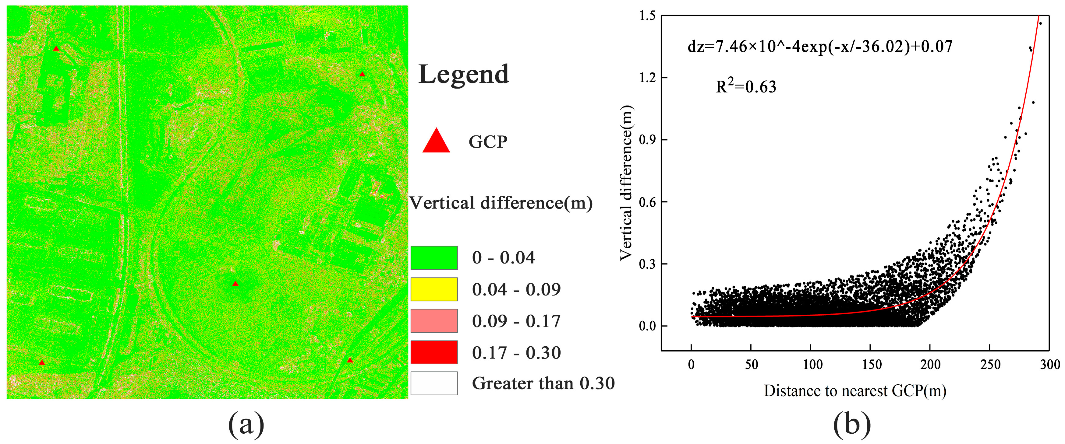
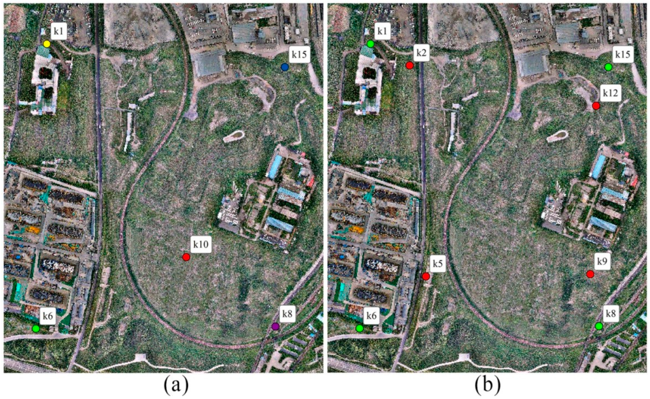
3.3. Influence of GCPs Distribution

The experimental results of evaluating the influence of the GCP distribution are shown in Figure 9. The box diagram represents the difference between the elevation of checkpoints and the elevation of the DSM extraction point. In the layout of one GCP, four tests (excluding K15) showed low variability, in which K10 was near the center of the region and the error was the smallest. In the experiments with different distributions of four GCPs, compared with the results of using K1, 6, 8, and 15, the error of using K2, 5, 9, and 12 was significantly reduced. The difference is that the distance between K2, 5, 9, and 12 decreased.
In addition, ArcGIS was used for differential calculations. The difference was assessed by subtracting the DSM produced using a uniform distribution of five GCPs and the DSM produced using the optimal distribution of 16 GCPs; the differential DSM resolution was 0.2 m (Figure 10a). The results show that when the distance from the nearest GCP increases, the DSM local vertical difference tends to increase. There are many scattered points in Figure 10b, indicating that the local DSM accuracy is not solely determined by the distance to the nearest GCP; therefore, a nonlinear curve is used for fitting.

4. Discussion

Using direct georeferencing can significantly improve the efficiency of UAV measurement. This study evaluated the geospatial accuracy of photogrammetric products obtained by direct georeferencing, and the impact of the configuration of GCPs on the quality of results. The RMSE, the M3C2 distance of the point cloud, the GCP distribution, and measures to improve the accuracy of the results when direct georeferencing are discussed below.
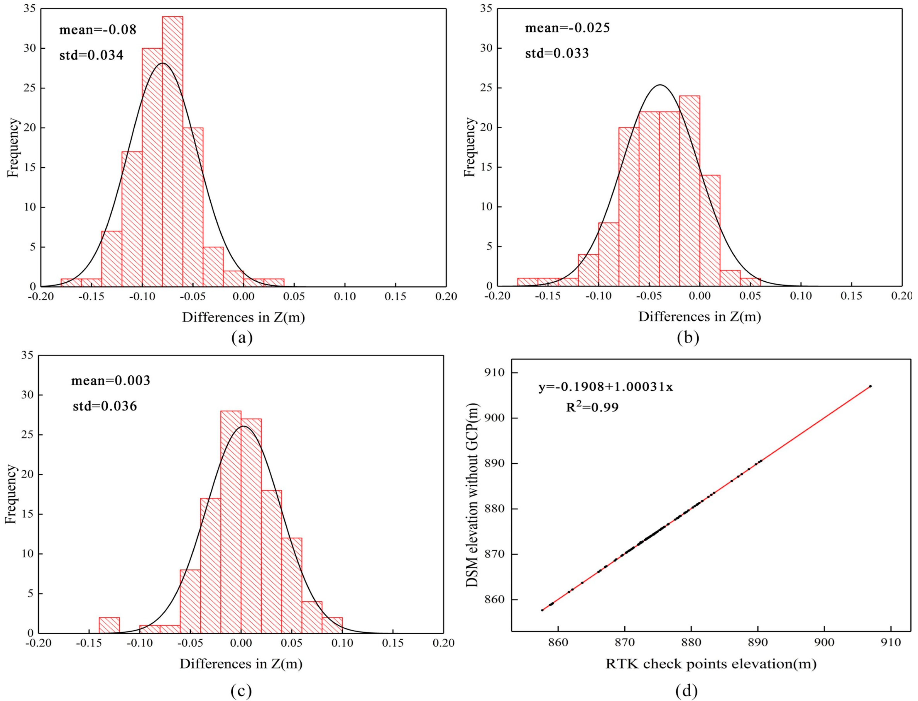
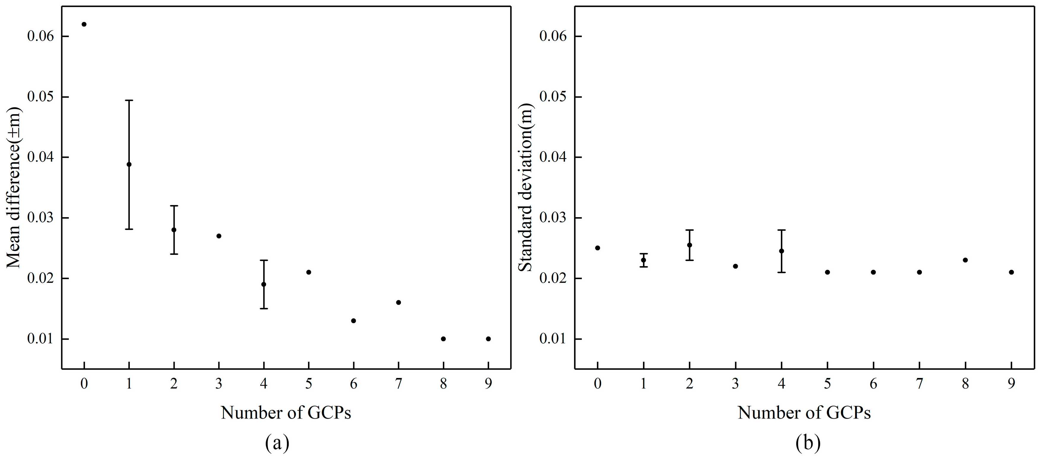
  • Error analysis based on the RMSE shows that adding one GCP can help to reduce the deviation, but there may still be dome error, as shown in the study of Rosnell and Javernick [27,38]. When two GCPs were used, the mean vertical difference was reduced to 0.003 m, and the horizontal RMSE was 0.0198 m, approximately 1.1 GSD, when 3 GCPs were used. From the work in some natural environments to the investigation of infrastructure, such as modelling water runoff during rain, different projects have different requirements for the fineness of ground features, so the required accuracy depends on the purpose of generating DSM. Therefore, using only one GCP may not meet the high accuracy standards; two to three GCPs are recommended for a trade-off between accuracy and work efficiency. The influence of each error on RMSE is directly proportional to the size of the square error, and therefore RMSE is sensitive to large differences and does not reflect terrain changes. Because of scale differences, errors that do not occur in flat areas may also occur in sloped areas [15]. The natural environment presents a series of complexities, including changing vegetation cover, strong topographic relief, and changes in texture. Future studies will need to assess the impact of these complexities on the accuracy of the results. Calculating RMSE is a common error assessment method when the actual dataset of the ground surface is a set of distribution points rather than a continuous, real surface. Error evaluation benefits from a larger number and more evenly distributed checkpoints. Gomes et al. arranged 270 vertical checkpoints in an area of about 0.22 km2, with a density of 1227 checkpoints per km2 [39]. In the study of Tomaštík, the density of checkpoints at the three sites was approximately 11363, 3674 and 2749 per km2 [8]. Thus, even if the number of GCP measurements on the ground is minimized, the role of checkpoints in the error assessment is critical. In the future, the plan is to deploy as many checkpoints as possible in the study area, build an accurate error surface, analyze the spatial distribution characteristics of errors, and better verify the results; these tasks will help to understand and reduce the potential error sources in the UAV SfM workflow [36];
  • The M3C2 algorithm eliminates the error introduced by the interpolation process. Lower error measurements with M3C2 are comparable to point-to-point or point-to-mesh; the method has been widely used in research based on point cloud change detection [40,41,42,43]. Due to the high point density of UAV matching point clouds, an intercomparison can actually be regarded as continuous [44]. At zero GCP, the M3C2 distance error shows randomness in the study area. The standard deviation range of the comparison between the reference point cloud and the point cloud of different projects is 0.021–0.028 m. The change is relatively small, and the point cloud only deviates in the vertical direction, which is similar to the study of Tomaštík and Štroner et al. [6,44]. Standard deviation is an indicator of precision. In some applications of UAV SfM, the accuracy of geolocation is not as important as the repeatability (precision) of data. For example, comparing multi temporal measurement data to study the change in terrain with time, more attention is paid to the relative change between data, and the quality of multi temporal data can be improved through cooperative registration;
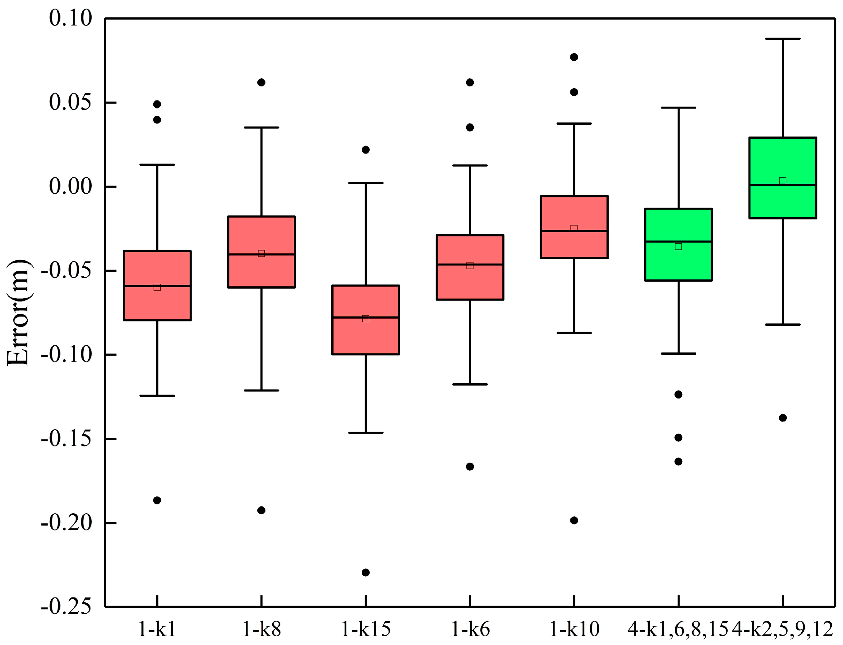
  • GCP distribution experiments show that the uniform distribution of GCPs is crucial when using more than one GCP. Figure 10b uses nonlinear curve fitting. In Gindraux’s study, linear fitting was used to determine that, on average, the vertical accuracy decreased by 0.09 m when the distance from the nearest GCP increased by 100 m [45]. In the experiment with four GCPs, the accuracy was improved after moving the GCP slightly towards the center of the study area compared with placing the GCP at the edge of the study area, which is similar to the study of Martínez. Martínez’s study concluded that the best horizontal accuracies are achieved by placing GCPs around the edges of the study area, but it is also essential to place GCPs inside the area with a stratified distribution to optimize vertical accuracy [28];
  • The DSM vertical RMSE and DOM horizontal RMSE obtained by direct georeferencing with the GSD set to 1.7 cm/pixel were 0.087 and 0.041 m, respectively. Without GCPs, the accuracy of the results was highly dependent on the accuracy of the image position data. The following measures can be taken to improve the accuracy of results obtained without GCPs. UAV cross flights and imagery with large overlap can provide redundant data and improve the reliability of image matching, which requires high computing power [1,39]. The addition of oblique images helps to accurately estimate the internal and external orientation elements in the process of bundle adjustment, extract vertical features such as building sidewalls, and obtain the best vertical accuracy [13]. A more accurate GCP measurement method can be used, rather than simply increasing the number of GCPs. Another recommendation is to use a tripod-mounted prism instead of a pole-mounted prism, as well as the RTK static measurement method when time permits. If inaccurate coordinates are introduced when measuring GCPs, a more complex error surface will be introduced, as opposed to reducing the initial deformation [14].
The direct georeferencing technology integrated by UAV and GNSS RTK has advantages in monitoring locations with large ranges or difficult access. However, further development is needed. High-quality optical lenses and multi-frequency GPS can obtain higher quality images and positioning accuracy.

5. Conclusions

In this study, the geospatial accuracy of photogrammetric products obtained by the FEIMA D2000 direct georeferencing method was evaluated using ground-measured data. In addition, we evaluated the effect of the quantity and spatial distribution of GCPs on the quality of the results. The research results are summarized as follows:
  • UAV SfM is a flexible and efficient method to obtain high-resolution topographic data. The direct georeferencing method based on the RTK/PPK fusion difference to obtain high-accuracy image positions has potential for improving the accuracy of the products, especially when GPS measurements are difficult, as well as reducing the dependence on the GCPs in the bundle adjustment, and decreasing the field work time and cost.
  • The research results show that the vertical RMSE of the DSM obtained by direct georeferencing was 0.087 m, approximately equal to 5.12 GSD. The horizontal RMSE of the DOM was 0.041 m, approximately equal to 2.41 GSD. Both values reached the centimeter positioning accuracy and achieve the application research of decimeter-error scale. The accuracy of UAV direct georeferencing could be guaranteed through careful flight planning, an appropriate survey, and accurate data post-processing. In the study of terrain change detection, we suggest evenly deploying two to three GCPs to achieve a good compromise between appropriate accuracy, repeatability and efficiency.
  • GCPs should be uniformly distributed in the study area and contain at least one GCP near the center of the domain to reduce the dome effect. With an increase in the number of GCPs in the bundle adjustment, both the horizontal error and vertical error decreased, and the horizontal error was always lower than the vertical error. When the density of the GCPs was greater than 12 GCP/km2 and 10 GCP/km2, respectively, the decrease in the vertical and horizontal errors was not obvious. The minimum vertical and horizontal RMSE were 0.032 (~1.88 GSD) and 0.015 m (~0.88 GSD), respectively.

Author Contributions

Conceptualization, X.L. (Xiaoyu Liu) and X.L. (Xugang Lian); methodology, X.L. (Xiaoyu Liu) and X.L. (Xugang Lian); software, F.W.; validation, F.W., Y.H. and Y.Z.; formal analysis, X.L. (Xugang Lian); investigation, X.L. (Xiaoyu Liu); resources, X.L. (Xugang Lian) and W.Y.; data curation, Y.Z.; writing—original draft preparation, X.L. (Xiaoyu Liu); writing—review and editing, X.L. (Xugang Lian); visualization, Y.H.; supervision, X.L. (Xugang Lian); project administration, W.Y.; funding acquisition, X.L. (Xugang Lian) and W.Y. All authors have read and agreed to the published version of the manuscript.

Funding

This research was funded by the National Natural Science Foundation of China, grant numbers 42101414 and 51704205; the Basic Applied Research Projects of Shanxi Province, grant number 201901D111466; the Key projects of Shanxi coal based low carbon joint fund of National Natural Science Foundation of China, grant number U1810203.

Institutional Review Board Statement

Not applicable.

Informed Consent Statement

Not applicable.

Acknowledgments

We would like to thank the reviewers for their helpful comments.

Conflicts of Interest

The authors declare no conflict of interest.

References

  1. Zhang, H.; Aldana-Jague, E.; Clapuyt, F.; Wilken, F.; Vanacker, V.; Van Oost, K. Evaluating the potential of post-processing kinematic (PPK) georeferencing for UAV-based structure-from-motion (SfM) photogrammetry and surface change detection. Earth Surf. Dyn. 2019, 7, 807–827. [Google Scholar] [CrossRef] [Green Version]
  2. Ullman, S. The interpretation of structure from motion. Proc. R. Soc. Lond. Ser. B Biol. Sci. 1979, 203, 405–426. [Google Scholar]
  3. Eltner, A.; Kaiser, A.; Castillo, C.; Rock, G.; Neugirg, F.; Abellán, A. Image-based surface reconstruction in geomorphometry–merits, limits and developments. Earth Surf. Dyn. 2016, 4, 359–389. [Google Scholar] [CrossRef] [Green Version]
  4. James, M.R.; Robson, S. Straightforward reconstruction of 3D surfaces and topography with a camera: Accuracy and geoscience application. J. Geophys. Res. Earth Surf. 2012, 117, F3. [Google Scholar] [CrossRef] [Green Version]
  5. Kim, D.-W.; Yun, H.S.; Jeong, S.-J.; Kwon, Y.-S.; Kim, S.-G.; Lee, W.S.; Kim, H.-J. Modeling and testing of growth status for Chinese cabbage and white radish with UAV-based RGB imagery. Remote Sens. 2018, 10, 563. [Google Scholar] [CrossRef] [Green Version]
  6. Tomaštík, J.; Mokroš, M.; Saloň, Š.; Chudý, F.; Tunák, D. Accuracy of photogrammetric UAV-based point clouds under conditions of partially-open forest canopy. Forests 2017, 8, 151. [Google Scholar] [CrossRef] [Green Version]
  7. Lian, X.; Li, Z.; Yuan, H.; Hu, H.; Cai, Y.; Liu, X. Determination of the Stability of High-Steep Slopes by Global Navigation Satellite System (GNSS) Real-Time Monitoring in Long Wall Mining. Appl. Sci. 2020, 10, 1952. [Google Scholar] [CrossRef] [Green Version]
  8. Godone, D.; Allasia, P.; Borrelli, L.; Gullà, G. UAV and Structure from Motion Approach to Monitor the Maierato Landslide Evolution. Remote Sens. 2020, 12, 1039. [Google Scholar] [CrossRef] [Green Version]
  9. Long, N.; Millescamps, B.; Guillot, B.; Pouget, F.; Bertin, X. Monitoring the topography of a dynamic tidal inlet using UAV imagery. Remote Sens. 2016, 8, 387. [Google Scholar] [CrossRef] [Green Version]
  10. Long, N.; Millescamps, B.; Pouget, F.; Dumon, A.; Lachaussée, N.; Bertin, X. Accuracy assessment of coastal topography derived from UAV images. Int. Arch. Photogramm. Remote Sens. Spat. Inf. Sci. 2016, 41, B1. [Google Scholar]
  11. Immerzeel, W.W.; Kraaijenbrink, P.D.A.; Shea, J.; Shrestha, A.; Pellicciotti, F.; Bierkens, M.F.P.; De Jong, S.M. High-resolution monitoring of Himalayan glacier dynamics using unmanned aerial vehicles. Remote Sens. Environ. 2014, 150, 93–103. [Google Scholar] [CrossRef]
  12. Mallalieu, J.; Carrivick, J.L.; Quincey, D.J.; Smith, M.W.; James, W.H. An integrated Structure-from-Motion and time-lapse technique for quantifying ice-margin dynamics. J. Glaciol. 2017, 63, 937–949. [Google Scholar] [CrossRef] [Green Version]
  13. Zeybek, M. Accuracy assessment of direct georeferencing UAV images with onboard global navigation satellite system and comparison of CORS/RTK surveying methods. Meas. Sci. Technol. 2021, 32, 065402. [Google Scholar] [CrossRef]
  14. Sanz-Ablanedo, E.; Chandler, J.H.; Rodríguez-Pérez, J.R.; Ordóñez, C. Accuracy of unmanned aerial vehicle (UAV) and SfM photogrammetry survey as a function of the number and location of ground control points used. Remote Sens. 2018, 10, 1606. [Google Scholar] [CrossRef] [Green Version]
  15. Cucchiaro, S.; Fallu, D.J.; Zhang, H.; Walsh, K.; Van Oost, K.; Brown, A.G.; Tarolli, P. Multiplatform-SfM and TLS data fusion for monitoring agricultural terraces in complex topographic and landcover conditions. Remote Sens. 2020, 12, 1946. [Google Scholar] [CrossRef]
  16. McMahon, C.; Mora, O.E.; Starek, M.J. Evaluating the Performance of sUAS Photogrammetry with PPK Positioning for Infrastructure Mapping. Drones 2021, 5, 50. [Google Scholar] [CrossRef]
  17. Padró, J.C.; Muñoz, F.J.; Planas, J.; Pons, X. Comparison of four UAV georeferencing methods for environmental monitoring purposes focusing on the combined use with airborne and satellite remote sensing platforms. Int. J. Appl. Earth Obs. Geoinf. 2019, 75, 130–140. [Google Scholar] [CrossRef]
  18. Nolan, M.; Larsen, C.; Sturm, M. Mapping snow depth from manned aircraft on landscape scales at centimeter resolution using structure-from-motion photogrammetry. Cryosphere 2015, 9, 1445–1463. [Google Scholar] [CrossRef] [Green Version]
  19. Tomaštík, J.; Mokroš, M.; Surový, P.; Grznárová, A.; Merganič, J. UAV RTK/PPK method—An optimal solution for mapping inaccessible forested areas? Remote Sens. 2019, 11, 721. [Google Scholar] [CrossRef] [Green Version]
  20. Erenoglu, R.C.; Erenoglu, O. A case study on the comparison of terrestrial methods and unmanned aerial vehicle technique in landslide surveys: Sarıcaeli landslide, Çanakkale, NW Turkey. Int. J. Environ. Geoinf. 2018, 5, 325–336. [Google Scholar] [CrossRef]
  21. Turner, D.; Lucieer, A.; Watson, C. An automated technique for generating georectified mosaics from ultra-high resolution unmanned aerial vehicle (UAV) imagery, based on structure from motion (SfM) point clouds. Remote Sens. 2012, 4, 1392–1410. [Google Scholar] [CrossRef] [Green Version]
  22. Shahbazi, M.; Sohn, G.; Théau, J.; Menard, P. Development and evaluation of a UAV-photogrammetry system for precise 3D environmental modeling. Sensors 2015, 15, 27493–27524. [Google Scholar] [CrossRef] [Green Version]
  23. Mian, O.; Lutes, J.; Lipa, G.; Hutton, J.J.; Gavelle, E.; Borghini, S. Accuracy assessment of direct georeferencing for photogrammetric applications on small unmanned aerial platforms. Int. Arch. Photogramm. Remote Sens. Spat. Inf. Sci. 2016, 40, 77. [Google Scholar] [CrossRef] [Green Version]
  24. Hugenholtz, C.; Brown, O.; Walker, J.; Barchyn, T.E.; Nesbit, P.; Kucharczyk, M.; Myshak, S. Spatial accuracy of UAV-derived orthoimagery and topography: Comparing photogrammetric models processed with direct geo-referencing and ground control points. Geomatica 2016, 70, 21–30. [Google Scholar] [CrossRef]
  25. Agüera-Vega, F.; Carvajal-Ramírez, F.; Martínez-Carricondo, P. Assessment of photogrammetric mapping accuracy based on variation ground control points number using unmanned aerial vehicle. Measurement 2017, 98, 221–227. [Google Scholar] [CrossRef]
  26. Tahar, K.N. An evaluation on different number of ground control points in unmanned aerial vehicle photogrammetric block. Int. Arch. Photogramm. Remote Sens. Spat. Inf. Sci. 2013, 40, 93–98. [Google Scholar] [CrossRef] [Green Version]
  27. Rosnell, T.; Honkavaara, E. Point cloud generation from aerial image data acquired by a quadrocopter type micro unmanned aerial vehicle and a digital still camera. Sensors 2012, 12, 453–480. [Google Scholar] [CrossRef] [Green Version]
  28. Martínez-Carricondo, P.; Agüera-Vega, F.; Carvajal-Ramírez, F.; Mesas-Carrascosa, F.J.; García-Ferrer, A.; Pérez-Porras, F.-J. Assessment of UAV-photogrammetric mapping accuracy based on variation of ground control points. Int. J. Appl. Earth Obs. Geoinf. 2018, 72, 1–10. [Google Scholar] [CrossRef]
  29. Reshetyuk, Y.; Mårtensson, S.G. Generation of highly accurate digital elevation models with unmanned aerial vehicles. Photogramm. Rec. 2016, 31, 143–165. [Google Scholar] [CrossRef]
  30. Stott, E.; Williams, R.D.; Hoey, T.B. Ground control point distribution for accurate kilometre-scale topographic mapping using an RTK-GNSS unmanned aerial vehicle and SfM photogrammetry. Drones 2020, 4, 55. [Google Scholar] [CrossRef]
  31. Lague, D.; Brodu, N.; Leroux, J. Accurate 3D comparison of complex topography with terrestrial laser scanner: Application to the Rangitikei canyon (NZ). ISPRS J. Photogram. Remote Sens. 2013, 82, 10–26. [Google Scholar] [CrossRef] [Green Version]
  32. Agisoft LCC. Agisoft PhotoScan. Available online: http://www.agisoft.com (accessed on 20 February 2017).
  33. Yu, Z.; Zhou, H.; Li, C. Fast non-rigid image feature matching for agricultural UAV via probabilistic inference with regularization techniques. Comput. Electron. Agric. 2017, 143, 79–89. [Google Scholar] [CrossRef]
  34. Jiang, S.; Jiang, W. On-board GNSS/IMU assisted feature extraction and matching for oblique UAV images. Remote Sens. 2017, 9, 813. [Google Scholar] [CrossRef] [Green Version]
  35. Snavely, N.; Seitz, S.M.; Szeliski, R. Modeling the world from internet photo collections. Int. J. Comput. Vis. 2008, 80, 189–210. [Google Scholar] [CrossRef] [Green Version]
  36. James, M.R.; Robson, S.; d’Oleire-Oltmanns, S.; Niethammer, U. Optimising UAV topographic surveys processed with structure-from-motion: Ground control quality, quantity and bundle adjustment. Geomorphology 2017, 280, 51–66. [Google Scholar] [CrossRef] [Green Version]
  37. CloudCompare v2.10.2. Available online: https://www.danielgm.net/cc/ (accessed on 18 July 2020).
  38. Javernick, L.; Brasington, J.; Caruso, B. Modeling the topography of shallow braided rivers using Structure-from-Motion photogrammetry. Geomorphology 2014, 213, 166–182. [Google Scholar] [CrossRef]
  39. Pessoa, G.G.; Carrilho, A.C.; Miyoshi, G.T.; Amorim, A.; Galo, M. Assessment of UAV-based digital surface model and the effects of quantity and distribution of ground control points. Int. J. Remote Sens. 2021, 42, 65–83. [Google Scholar] [CrossRef]
  40. Stumpf, A.; Malet, J.P.; Allemand, P.; Deseilligny, M.P.; Skupinski, G. Ground-based multi-view photogrammetry for the monitoring of landslide deformation and erosion. Geomorphology 2015, 231, 130–145. [Google Scholar] [CrossRef]
  41. Cucchiaro, S.; Cavalli, M.; Vericat, D.; Crema, S.; Llena, M.; Beinat, A.; Marchi, L.; Cazorzi, F. Monitoring topographic changes through 4D-structure-from-motion photogrammetry: Application to a debris-flow channel. Environ. Earth Sci. 2018, 77, 632. [Google Scholar] [CrossRef]
  42. Milan, D.J.; Heritage, G.L.; Large, A.R.G.; Fuller, I.C. Filtering spatial error from DEMs: Implications for morphological change estimation. Geomorphology 2011, 125, 160–171. [Google Scholar] [CrossRef]
  43. Cook, K.L. An evaluation of the effectiveness of low-cost UAVs and structure from motion for geomorphic change detection. Geomorphology 2017, 278, 195–208. [Google Scholar] [CrossRef]
  44. Štroner, M.; Urban, R.; Reindl, T.; Seidl, J.; Brouček, J. Evaluation of the georeferencing accuracy of a photogrammetric model using a quadrocopter with onboard GNSS RTK. Sensors 2020, 20, 2318. [Google Scholar] [CrossRef] [PubMed] [Green Version]
  45. Gindraux, S.; Boesch, R.; Farinotti, D. Accuracy assessment of digital surface models from unmanned aerial vehicles’ imagery on glaciers. Remote Sens. 2017, 9, 186. [Google Scholar] [CrossRef] [Green Version]
Figure 1. Workflow of methods, starting with the route planning of a UAV campaign until the determination of DSM and orthomosaic accuracy (RMSE and M3C2 distance).
Drones 06 00030 g001
Figure 2. Study area with the GCP and checkpoint distributions. Projection coordinate system: WGS_1984_UTM_zone_49N; (a) DOM and (b) route map.
Drones 06 00030 g002
Figure 3. Experimental settings. (a) FEIMA D2000 UAV. (b) Distribution of GCPs and CPs in the bundle adjustment. (c) Measurement of field control points. (d) Display of control points in the image. (e) The number of overlapping images used in each pixel calculation. Red and yellow areas indicate low overlap, while green areas indicate more than 5 images per pixel.
Drones 06 00030 g003
Figure 4. Schemes with different distributions of GCPs. (a) Five distributions of one GCP; (b) two distributions of four GCPs. The distributions are shown by different colours.
Drones 06 00030 g004
Figure 5. Effect of GCP density on the RMSE of (a) DSM vertical and (b) DOM horizontal. GCP density was calculated by dividing the quantity of GCPs used by the measurement area of 0.5 km2. d represents the density of point clouds on the horizontal axis. Add error bars at ±1 standard error at GCP density of 2, 4 and 8, respectively.
Drones 06 00030 g005
Figure 6. Statistical analysis of the UAV survey based on 120 checkpoints. (ac) Histograms of elevation differences between the DSM and RTK checkpoints obtained by 0, 1, or 2 GCPs and their Gaussian fit. (d) Linear fitting function between RTK checkpoint elevations and DSM elevations obtained with 0 GCPs.
Drones 06 00030 g006
Figure 7. M3C2 distance between reference point clouds (16 GCPs) and point clouds obtained from different photogrammetric projects. (a) Average difference (accuracy). (b) Standard deviation (precision). Add error bars at +/−1 standard error at GCP number of 1, 2 and 4, respectively.
Drones 06 00030 g007
Figure 8. M3C2 distance between the point cloud obtained by using different numbers of GCPs as control points and the reference point cloud (obtained by using all 16 GCPS). (ad) Zero-, 3-, 6-, and 9-GCP and Gaussian distribution. Solid black dots indicate the location of GCPs. The vertical red line in the figure are zero error lines.
Drones 06 00030 g008
Figure 9. Boxplots represent vertical errors obtained by seven layout schemes divided by the number of GCPs (the horizontal line represents the median, the lower part of the hinge represents the 25th percentile, and the upper part represents the 75th percentile). The whiskers represent 1.5× IQR (interquartile range) in both directions. The black squares and circles represent the mean and outliers, respectively. Refer to the schematic diagram of different GCP distribution in Figure 4. 1 and k1 in 1-k1 represent the number and code of control points respectively, and others are similar.
Drones 06 00030 g009
Figure 10. Relationship between local DSM accuracy and nearest GCP. (a) Differential DSM; (b) the scatterplot and nonlinear curve fit obtained by sampling from the differential DSM.
Drones 06 00030 g010
Table 1. Technical specifications of the UAV platform.
UAV BodyD-CAM2000 Aerial Module
System standard takeoff weight2.8 kgCameraSONY a6000
Standard load200 gEffective pixels24.3 million
Endurance74 minSensor23.5 × 15.6 mm (aps-c)
Remote control distance20 km (max)Focal length25 mm
Table 2. Single sample t-test results.
Number of GCPstDegree of FreedomSignificanceMean Difference Value95% Confidence Interval
Lower LimitUpper Limit
1−8.1751193.64 × 10−13−0.025−0.031−0.019
20.7601190.4490.003−0.0040.009
Table 3. M3C2 distance values between reference point clouds and point clouds obtained by GCPs with different numbers and distributions. Refer to Figure 4 to identify these points.
ProjectMean (m)std (m)ProjectMean (m)std (m)
16-00.0620.02516-30.0270.022
16-1/k10.0460.02316-4/k2,k5,k9,k12−0.0150.028
16-1/k80.0230.02216-4/k1,k6,k8,k150.0230.021
16-1/k150.0530.02516-50.0210.021
16-1/k100.0410.02316-60.0130.021
16-1/k60.0310.02216-70.0160.021
16-2/k1, k100.0320.02316-80.010.023
16-2/k6, k150.0240.02816-90.010.021
Publisher’s Note: MDPI stays neutral with regard to jurisdictional claims in published maps and institutional affiliations.

