Abstract
Bottle marine debris (BMD) remains one of the most pressing global issues. This study proposes a detection method for BMD using unmanned aerial vehicles (UAV) and machine learning techniques to enhance the efficiency of marine debris studies. The UAVs were operated at three designed sites and at one testing site at twelve fly heights corresponding to 0.12 to 1.54 cm/pixel resolutions. The You Only Look Once version 2 (YOLO v2) object detection algorithm was trained to identify BMD. We added data augmentation and image processing of background removal to optimize BMD detection. The augmentation helped the mean intersection over the union in the training process reach 0.81. Background removal reduced processing time and noise, resulting in greater precision at the testing site. According to the results at all study sites, we found that approximately 0.5 cm/pixel resolution should be a considerable selection for aerial surveys on BMD. At 0.5 cm/pixel, the mean precision, recall rate, and F1-score are 0.94, 0.97, and 0.95, respectively, at the designed sites, and 0.61, 0.86, and 0.72, respectively, at the testing site. Our work contributes to beach debris surveys and optimizes detection, especially with the augmentation step in training data and background removal procedures.
1. Introduction
Estimating bottle marine debris (BMD) on beaches, as well as many other types of marine pollution, has become an urgent issue due to high quantities and potential hazards. BMD remains one of the top ten marine debris items removed from global coastlines and waterways [1,2]. Polyethylene terephthalate (PET) bottles pose a risk of “estrogenic” damage to human beings [3,4,5]. Hence, assembling quantitative data on BMD loads on beaches is critical from an environmental standpoint.
Until recently, visual census has been the primary method in related studies of marine debris [6,7,8]. However, some studies have noted notable drawbacks to this approach, such as over-subjective recognition, immoderate time and labor consumption, and constrained area coverage [9,10,11]. Meanwhile, some recent studies have implemented satellite images to save time and expand research space. However, image resolution is insufficient to facilitate recognizing objects such as average-sized bottles (5 to 50 cm) [12,13]. Hence, there is a need for approaches in remote monitoring and optimization of the detection efficiency in marine debris studies.
To overcome these shortcomings, Martin et al. (2018) [11] suggested a novel approach involving the use of unmanned aerial vehicles (UAVs) and machine learning techniques for automatic detection and quantification of marine debris. The method has since been advanced and expanded to other studies [11,14,15,16]. The object detection system as a random forest was implemented by integrating a histogram of oriented gradients (HoG) [11] with three additional color spaces [17]. Martin et al. (2018) compared the performance of three methods: standard visual census, manual screening, and automatic recognition and classification; the outcomes emphasized that the proportion of categories, excluding small items, from the three approaches was not significantly different [11]. Gonçalves et al. (2020) improved the accuracy of object identification for mapping marine litter on a beach dune system using techniques of the centroid of automatic output and manual procedure output [15]. Fallati et al. (2019) used commercial software with a deep learning convolutional neural network as its basic algorithm to recognize plastic debris [14]. Kako et al. (2020) employed a deep learning model based on the Keras framework to estimate plastic debris volumes [16]. Martin et al. (2021) estimated litter density on shores by developing a Faster R-CNN [18]. Takaya et al. (2022) employed the RetinaNet integration with non-maximum suppression to enhance the efficiency of debris detection [19]. Maharjan et al. (2022) created a plastic map of rivers by implementing different detection models in the You Only Look Once (YOLO) family [20]. Although pioneering works have highlighted the efficiency and broad applicability of machine learning in observing marine debris, they have also suggested different altitudes and resolutions in terms of operation. For instance, 10 m (0.5–0.7 cm/pixel) in Martin et al. (2018), 10 m (0.44 cm/pixel) in Fallati et al. (2019), 20 m (0.55 cm/pixel) in Gonçalves et al. (2020), 17 m (0.5 cm/pixel) in Kako et al. (2020), 10 m (0.27 cm/pixel) in Martin et al. (2021), 5 m (0.11 cm/pixel) in Takaya et al. (2022), and 30 m (0.82 cm/pixel) in Maharjan et al. (2022). These variations in fly height were primarily based on coverage, flight time, number of images, and subjective image quality assessment. Remarkably, object detection performance was not assessed. The optimal resolution range of aerial images for surveys to achieve the highest efficiency in marine debris research remains elusive.
Therefore, this study aims to determine the considerable range of image resolution in a UAV-based approach to enhance the efficiency of BMD research or marine debris. The experiments were implemented on a sandy beach sector of Taoyuan, Taiwan. We organized three designed sites for setting up training datasets, a testing algorithm named You Only Look Once version 2 (YOLO v2), and a testing site to observe our approach on a complex sandy beach. At each study site, UAVs hovered and took aerial photos at different fly heights, and the range of optimal resolutions was determined based on the evaluation of detecting performance across four indices. We further proposed some methods to overcome the data limitations in machine learning that we encountered.
2. Materials and Methods
2.1. Study Area
Taoyuan beach, situated on the northwestern coast of Taiwan, is a region that requires unique conservation, especially when considering marine debris issues. The intertidal algal reefs are the ecological highlights on this coast, which host rich marine biodiversity and are essential ecosystems [21,22]. Coastal debris, particularly BMD, is one of the damaging factors for organisms by entanglement and “estrogenic” damage, as previously mentioned.
In this study, we conducted four cohesionless extents on a sandy beach of Taoyuan. We set up case study areas with a range of 10 m by 15 m, consisting of three designed sites (25°4′44.60′′ N, 121°9′8.84′′ E; 25°4′41.34′′ N, 121° 8′53.21′′ E; 25° 4′38.60′′ N, 121° 8′37.57′′ E) and a testing site (25° 4′27.12′′ N, 121°7′44.76′′ E). Figure 1a shows the geographic locations of the sector of Taoyuan beach, and Figure 1b shows a detailed map with the sites marked as small red rectangles. Figure 1c shows a closed-sight view at designed site 1. The testing site (Figure 1d) near the landfill area of Taoyuan City was used to judge our method on such a complex sandy beach. We surveyed a supratidal zone and neglected the intertidal zone because marine debris in the intertidal zone was dominated by sizes ranging from 0.2 cm to 2 cm [23], while this research only considered BMD as mentioned.
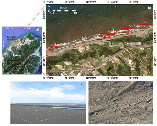
Figure 1.
Location and overview of the study sites. (a) Position of the study region in Taiwan, a sector of Taoyuan beach marked as a red rectangle; (b) detailed map of the study sites (red rectangles); (c) the designed site 1 overview taken during the field experience, with the drone and an aerial view of the beach; (d) the testing site overview from UAV flight.
2.2. Survey Method
Our field surveys were conducted at designed sites on 27 August 2020 and 6 December 2021, and the testing site was surveyed on 5 November 2021. Once on site, the surveyors marked the study area at a size of 10 m by 15 m. The ancillary data, such as the time, season, summary of current weather conditions, and environmental features, were simultaneously recorded. Three designed sites were cleaned before 85, 45, and 42 bottles were randomly arranged in four different states following the standard procedures: (1) placed intact on the beach surface, (2) partially buried in the ground, (3) overlapped or clustered together, and (4) deformed by impact. Notably, designed site 1 was first set up for accumulating datasets to train and test our detection approach.
For collecting aerial images, two quadcopters, a DJI Mavic 2 Professional (M2P) and a DJI Phantom 4 Professional (P4P), were employed. The drones were equipped with a camera sensor of 1-inch complementary metal oxide semiconductor (CMOS) with a 12.83 mm width and a 20-megapixel camera fixed on a three-axis gimbal. The P4P had a lens of 24 mm focal length and a mechanical shutter supporting the capture of 4K at 60 fps. The M2P camera had a 28 mm lens and a rolling shutter recording 4K video. The GPS/GLONASS satellite system helped both UAVs attain a hovering accuracy range of ±0.5 m vertical and ±1.5 m horizontal with GPS positioning status. The two drones captured images every 5 m at fly heights ranging from 5 m to 60 m. The UAVs were operated in a hovering mode (approximately stationary) that could minimize the motion of the camera and reduce the blurring effects on the captured images. However, it was noted that blurring effects might be an important issue in the case of real-time surveys. The oblique-view reconnaissance caused a significant effect on object coordinates [24] and on the object shapes due to radiometric and geometric deformations [25]. Therefore, the camera was tilted with a heading of 90 degrees toward the ground while capturing images [14,17,26]. The image area was based on image size and resolution, where the corresponding image resolutions were defined as:
where SW is the sensor width, FH is the flight height, FL is the focal length of the camera, and IW is the image width [14,27]. Hence, the image resolutions were from 0.12 to 1.54 cm/pixel. The image resolution changed with the flight altitude, as shown in Figure 2.
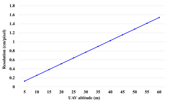
Figure 2.
The relation between the image resolution and the flying altitude of the UAV.
2.3. Machine Learning Procedure
This research employed the You Only Look Once version 2 (YOLO v2) convolutional neural network as the object detection system for BMD detection. YOLO v2 was created by Joseph Redmon and Ali Farhadi in 2017 [28]. The YOLO v2 was chosen because this model has been proven to be a useful tool to identify marine debris with satisfactory accuracy and computing speed. YOLO v2 has been applied in many studies in recent years [29,30,31,32]. In addition, the YOLO v2 achieves a score of 78.6 on mean average precision on testing the well-known dataset of Pascal VOC 2007, which is the best among many other models [28]. Notably, other new models (e.g., YOLO v7) have recently been developed; future works on testing how these new models improve the performance of identifying marine debris could contribute to the detection of marine debris.
YOLO v2 uses anchor boxes to detect objects in an image. Anchor boxes are predefined boxes that best match the given ground truth boxes and are defined by K-mean clustering. The anchor boxes are used to predict bounding boxes [28]. Estimating the number of anchor boxes is an important step in producing high-performance detectors [33]. Processing images with YOLO v2 has three main parts: (1) resizing the input image to size 416 × 416 pixels; (2) conducting a single convolutional network on the image; and (3) thresholding the resulting detections by the model’s confidence. Every input image is divided into an S × S grid of cells after resizing and predicts a fit B number of “bounding boxes”, “confidence scores” of those boxes, and C class probabilities. Each bounding box consists of five predictions: x, y, w, h, and confidence; where (x, y) are the center coordinates of that box, w and h correspond to its width and height. The confidence is calculated based on Formula (2), where Pr(object) is the probability of the object in the current grid and represents the intersection over union (IoU) between the predicted box and the ground truth box. After obtaining those predicted boxes, the output predictions of an input image will be encoded as an S × S × (B ∗ 5 + C) tensor. As only one category (BMD) is considered, we used C as equal to 1.
To save training time, the YOLO v2 system first automatically resizes images into 416 × 416 pixels, but it includes a flaw in changing image resolution and reducing the pixel information. Therefore, we created a simple application for image segmentation and anchor design. Each training image was divided into segments according to the desired size, and ground truth boxes were then hand-marked to gradually store their information, including image geolocation, BMD coordinates, and image size. Our effort contributes to ensuring the obviousness of training images, increasing pixel information of training data, and reducing the ability to misidentify natural items as debris.
In our training data procedure, as depicted in Figure 3a, twenty aerial photos taken at 0.12 cm/pixel resolution on designed site 1 were accumulated as an image source. This selection was conducted based on objects’ obviousness and the continually changing direction of UAVs, allowing BMD to be captured in various forms. Those images were first applied in our created application with the desired size at 1400 × 1400 pixels, corresponding to 0.42 cm/pixel resolution in the training procedure, and 624 segments and their information were totally produced for the training datastore. Eighty percent of the data were randomly selected for training, while the rest were used to test the usability of the model. The data augmentation, our additional phase, was extended in this procedure to overcome the limitation of the data quantity. Each segment was changed by flipping and adjusting the brightness (Figure 3b). As a result, the source quantity was enlarged to four times higher, which meant that every segment had four versions: original, bright, dark, and changing direction. The settings in the YOLO were then modified during every training run with inputs of different hyperparameters of minibatch size, initial learning rate, and max epochs (Table 1). We used seven anchor boxes for training in this study. The YOLO v2 was applied to the training and testing sets at different runs or with different training settings. After this step, the model which had good performances was used for detecting objects; hereafter, we call the framework/procedure of the overall object detection a “detector”.
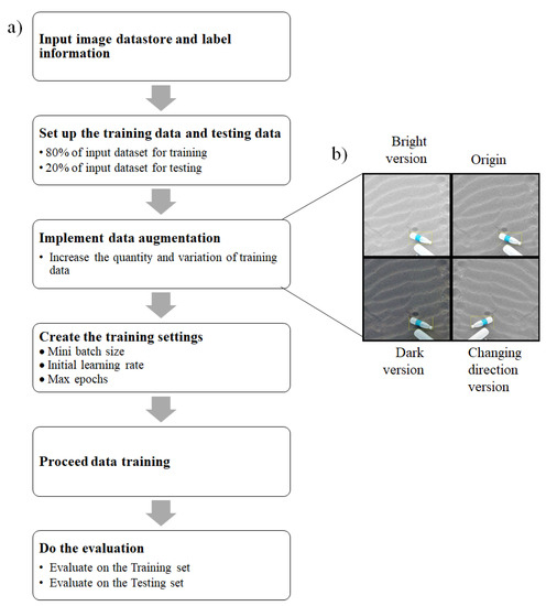
Figure 3.
Machine learning procedure. (a) Flowchart of the procedure; (b) example of image augmentation results.

Table 1.
Training hyperparameter values.
2.4. Background Removal
One challenge of automatic detection is the influence of the background environment, and background removal has been suggested in some research related to this topic to enhance training products and analysis accuracy. Some suggested approaches include the local binary pattern-based approach [34], hybrid center–symmetric local pattern feature [35], multi-Bernoulli filter [36], and analyzing the temporal evolution of pixel features to possibly replicate the decisions previously enforced by semantics [37]. To enhance automatic detection, these approaches have been widely applied in research related to object detection or even for detecting moving obstacles [38,39,40,41,42].
In this study, every raw image was first changed to a gray level to unify all the pixel indices, and then the Gaussian filter and local standard deviation filter were applied before creating a binary mask according to closed polygons (Figure 4a). The two filters were applied to smooth out the sandy background and enhance the edges of the items inside. Those edges were extended and highlighted by image dilation to shape more closed polygons, and a binary image was aimed at covering the image background. Consequently, the background removal image was proposed to focus on BMD within a scene. We implemented two different types of image source for training: original image (Figure 4b) and background removal image (Figure 4c).
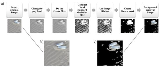
Figure 4.
Process of background removal. (a) Flow chart of the procedure; (b) example of the original image. (c) Example of the background removal image.
2.5. Detecting Process
This study performed three stages of analysis to examine for both original or background removal images: (1) it was divided into segments; (2) the detection was performed via 57 detectors; and (3) validated with reference data (Figure 5a). To ensure the resolution between the training data and the input image were the same, the segment size was first calculated according to the correlation between the actual border range of the training data and the segment’s resolution B (Figure 5b). Notably, threshold control is the supplementary phase of detecting items in background removal images to shorten the time. This phase was conducted according to the color histogram of segments; a segment with a histogram lower than the threshold was omitted to identify the following items. The whole processing time (T) was determined to compare the detection performance between two image types.
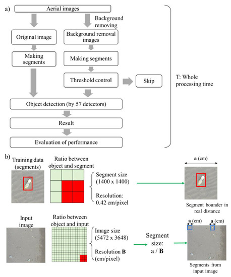
Figure 5.
Detecting procedure. (a) Flowchart of the detailed workflow. (b) Procedure for making segments of input images.
2.6. Performance Assessment
Training and detection performance was validated by four indices: intersection over union (IoU), precision, recall rate, and F1-score. IoU was set to measure the spatial ratio between the predicted box A (detected box) and ground truth box B as Formula (3) [43], and this was the critical index for validating trained models. This study used a 0.5 IoU threshold, in line with other studies [44,45,46,47,48]. In other words, every positive detection result was defined when the IoU was 0.5 or higher.
To evaluate the detection performance, each image used for automatic detection was visually screened in the GIS environment, and the objects identified as BMD were simultaneously hand-marked. The objects detected by the detector and by image screening were compared with each other via their overlap, and the match determined the detecting outcome as true positive (TP), false positive (FP), or false negative (FN).
To assess the detection performance, precision (4) is the ratio of the correctly predicted objects over the actual number of BMD:
Recall (5) is the proportion of correctly marked items from the total detections:
Both precision and recall failed to capture the whole picture of the detecting performance, so we measured the F1-score, which is “the harmonic mean of precision and recall” [49]:
3. Results
3.1. Performance of the Augmentation Phase
The image datasets before and after background removal were separately trained. Figure 6 shows an example of the loss reduction curve. For the three values of initial learning rate (10−3, 10−4 and 10−5), we found that the model was unstable during the training process when the initial learning rate was 10−4. When the initial learning rate was 10−3 and 10−5, the loss curve was steady with small fluctuation. The training loss value decreased when the number of epochs increased, and final average loss varied from 0.28 to 1.02.
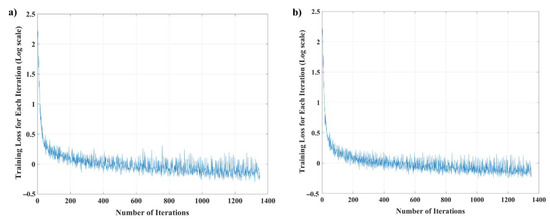
Figure 6.
Example of loss reduction curve (log scale) during the training process at 50 max epochs, mini-batch size at 8, and initial learning rate at 10−5. (a) Training loss and the number of iterations for original image dataset, (b) training loss and the number of iterations for background removal dataset.
Data augmentation was our additional phase in the training process, as previously mentioned. Table 2 compares the performance of this supplementary phase in both image types according to the IoU, precision, recall rate, and F1-score values described in Section 2.5. Except for precision, all ratios belonging to processes with the augmentation phase were greater. The model made from background removal images obtained the highest IoU at approximately 0.81. The best evaluation results were from training data; models made from the original image source and augmentation phase obtained a mean IoU, precision, recall and F1-score of about 0.78, 0.98, 0.0.97, and 0.98, respectively. The overall worst was the outcome of the testing data, with datasets made by the original image source and without the augmentation step. Furthermore, the precision measures of the models without augmentation were close to 1 because of the low number of samples, as well as the high power of YOLO v2. Table 2 emphasizes that, in all kinds of image sources, the performance of the process with the augmentation phase is better in both the training and testing data.

Table 2.
Comparison of training results with and without the augmentation phase (unit: mean ± std, aug: augmentation).
Fifty-seven models were trained with or without the augmentation phase, and we selected all of those models for detecting BMD. Hereafter, those models are called “detectors”. Because the objects of the marine debris might be complicatedly distributed in real-world situations, a small number of detectors might not have good performance in various conditions. Therefore, 57 detectors with different initial parameter settings were trained in different runs to increase the randomness. The results from the 57 detectors were then compared to evaluate the performance of these initial settings.
3.2. Performance at Designed Sites
The detection results at the three designed sites were measured as the mean values and are illustrated in Figure 7 via indices of precision, recall, and F1-score. The mean precision at all designed sites fluctuated between 0.8 and 1, especially that of designed site 1, which remained at approximately 0.9 as the location of the training data source. These good ratios may be due to the segmentation step’s effect in the object detection process (Section 2.4). The mean recall and mean F1-score values of the original images were higher than those of the background removal images at most resolutions; this showed a better performance of the original images at each site. Considerably, both recall and F1-score had a downward trend by 0.57 and 0.39 at designed site 1, by 0.55 and 0.52 at designed site 2, and by 0.66 and 0.67 at designed site 3, respectively, and a significant decrease by over 0.3 in both those indices of designed site 2 and designed site 3 compared to designed site 1, indicating the influences of environmental factors and sample conditions on the detection performance.
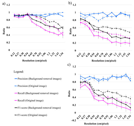
Figure 7.
Detection results at three designed sites. (a) Mean detection results at designed site 1; (b) mean detection results at designed site 2; (c) mean detection results at designed site 3. The error bars quantify standard deviations.
Each study area has a large variation in the range from 0.12 to 0.65 cm/pixel resolution; the remarkable peaks of mean precision, recall rate, and F1-score are 0.94, 0.97, and 0.95, respectively, at designed site 1 when the resolution is 0.54 cm/pixel; 0.85, 0.77, and 0.80, respectively, at designed site 2 when the resolution is 0.27 cm/pixel; and 0.81, 0.82, and 0.81, respectively, at designed site 3 when the resolution is 0. 27 cm/pixel. Therefore, resolutions between 0.3 and 0.5 cm/pixel should be the best choice for the resolution range at the designed sites. In contrast, background removal images show their high efficiency in detecting time: particularly faster than 0.09 s to over 2.83 s at designed site 1; more rapid than approximately 0.23 to nearly 3.33 s at designed site 2; and quicker than approximately 0.68 to 3.74 s at designed site 3 (Figure 8). In summary, while the original images at the three designed sites have better detection performance in the indices of recall and F1-score, the background removal images show their efficiency in saving more time.

Figure 8.
Mean detection time of 57 detectors on images with and without background removal at (a) designed site 1, (b) designed site 2, and (c) designed site 3. The error bars quantify standard deviations.
3.3. Performance at Testing Site
The outcomes at our testing site are noticeably different from those of the designed sites. Precision values of background removal images and original images increase by 0.26 and 0.23, respectively, in the testing site (Figure 9). This increase is due to the change in obviousness by resolutions, which means the more significant the image resolution, the clearer the objects. Furthermore, the occurrence of other items (noise) in the background are the same as some effects, such as sunlight, sand cover, and shadows, and is more obvious in high resolution.
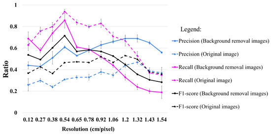
Figure 9.
Detection results of 57 detectors on images with and without removal at the testing site. Note that errors explain the standard deviation.
Furthermore, background removal images perform better in the testing site, particularly from 0.12 to 0.65 cm/pixel resolution (Figure 9). The precision values of the background removal images are larger by approximately 0.23 and 0.05 than those of the original images, while their F1-scores are greater by at least 0.06. Remarkably, background removal images obtain a local peak at 0.54 cm/pixel resolution, and the occurrence ratios of mean precision, recall rate, and F1-score are 0.61, 0.86, and 0.72, respectively. Comparing the range of recommended resolution (0.3 to 0.5 cm/pixel), which is described in Section 3.2, we selected approximately 0.5 cm/pixel as a highly suggestive resolution for aerial surveys related to BMD research. Background removal images also dominate in processing time at all resolutions, and they are faster from 0.88 to 31 s (Figure 10).
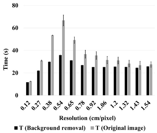
Figure 10.
Mean detection time of 57 detectors on images with and without removal at the testing site. Error here explains the standard deviation.
4. Discussion
4.1. Effects on the Detection Performance
Image types and landscape features are the two critical factors that influence BMD detection, and this was demonstrated by the difference in detection performance between background removal images and original images, as well as across study sites. At the designed sites, background removal images revealed lower values in recall rates and F1-scores, because of some misdetection (FN) in the background removal performance. A few bottles were removed through filtering in the background removal process due to the similar color between items and sand, or due to the diffuse boundaries when they were partially covered with sand, clustered together, or reflected by light. Examples of FN results are shown in Figure 11, where a bottle removed in filtering is marked by a red ellipse. In this image, a bottle removed after filtering while subtracting the background was marked with a red ellipse, and a misdetection bottle in both types of images was marked with green circles. Furthermore, YOLO v2 can work well in areas with a similar background to its training data. In this context, the sandy coast at designed site 1 (training source) and designed sites 2 and 3 (two evaluating areas) were quite similar. Therefore, the original images were more dominant in detecting BMD at the designed sites.
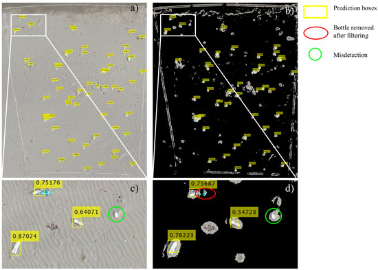
Figure 11.
Example of FN on images with and without background removal at designed site 1 at 1.06 cm/pixel resolution. Detecting results on the original image (a) and background removal image (b) are marked as yellow boundary boxes, while (c,d) are, respectively, the closed view sight corresponding to the white areas in the two above.
Landscape features at the testing site were remarkably different from those at designed site 1 (training data source), which caused a significant change in detection performance. The analysis results of the background removal image dominated the precision, F1-score, and processing time, while the outcomes of the original images were significantly dispersed. Specifically, in the initial resolution range from 0.12 to 1.06 cm/pixel, the recall index compared to the precision on the original image was more than double, even more than triple, at a resolution of 0.38 cm/pixel. This contradiction can be explained based on the high noise (e.g., change in sunlight, footprints, wooden sticks, plastic bags, styrofoam boxes, and shadows), which were misidentified as BMD on the beach landscape, and those FP outcomes are indicated in Figure 12. Therefore, operating surveys under similar solar conditions can reduce the influence of light, darkness, and environmental conditions on analysis outcomes, consistent with other studies [14,17]. According to the much lower density of noise and FP in the background removal image than in the original image in Figure 12, we believe that our suggestion regarding the background removal process is a more radical solution that boosts detection efficiency. In other words, the background removal image has the potential for application in study regions with many influencing factors.
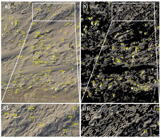
Figure 12.
Example of noise and FP on images with and without background removal at the testing site. Detection result on the original image (a) and background removal image (b) at 0.54 cm/pixel resolution are marked as yellow boundary box, while (c,d) are, respectively, the closed view sight corresponding to the white areas in the two above. These zoomed views indicate that some objects, particularly footprints, wooden sticks, styrofoam boxes, and shadows, were mistakenly identified as BMD.
To enhance the automatic detection efficiency, the data augmentation phase was supplemented in the training process, and the image segmentation step was applied in both the training and detection processes. Despite those efforts, the two issues of FN and FP were still obtained in both image types at all study sites (Figure 11 and Figure 12), and the low number of training samples was, we believe, the leading cause of these issues. To mitigate these weaknesses and optimize the capacity of the machine learning algorithm, we intend to conduct two future development strategies: (1) increasing the quantity of training data by surveying wider regions with various beach terrains; and (2) developing the data augmentation phase by supplementing more transformation versions of different light levels and rotational directions.
As time savings were one of the key purposes of utilizing machine learning in research of marine debris, the detection time on the two image types was compared with each other in this context, and the background removal image was again underlined in high research efficiency. At all study sites, the background removal images obtained results more quickly than the original images, and the difference was significant at the testing site (Figure 10 and Figure 12). The threshold control step in the detection process (Section 2.4) was our method to reduce the time consumption, and it was set up on background removal images due to the great difference between the background and object colors. There is no doubt that the background removal process is feasible, both to save analysis time and to increase BMD recognition efficiency.
4.2. The Potential Approach and Future Improvements
Recent works have applied and simultaneously evaluated the effectiveness of automatic detection by machine learning. Some notable results have been highlighted, and some outcomes are consistent with this study. Martin et al. pointed out that the proportion of categories (excluding small items) in detection and classification was not significantly different from the visual census method [11]. In terms of performance, the precision, recall rate, F1-score, and other parameters used in previous studies are listed in Table 3 to compare with the setting of our study. Despite using just 624 segments for training data, the performance of our work at designed sites obtained high efficiency, and the performance at the testing site was quite similar to that of Golcaves et al. (2020) [17] and Takaya et al. (2022) [19].

Table 3.
Main materials and outcomes of prior research related to BMD via machine learning and this work.
In the planning of the study, we attempted to add complexities that would match real-world situations. For example, different colors and sizes (from 5 to 50 cm) of marine bottles were used in the training process. Fifty-seven detectors were used to increase the randomness in the auto-detection process. Detection algorithms and analysis procedures were also tested and studied in both the designed and testing (real-world) sites. The results indicated that resolution was an significant factor that definitely affected the performance of detection. We also found that the image resolution used in other studies ranged from 0.11 to 0.82 cm/pixel (Table 3), and many studies used a resolution of around 0.5 cm/pixel in their surveys. As a result, a resolution of 0.5 cm/pixel could be a considerable choice that has potential application in large-scale surveys.
The main limitation of this study was that the detector we used was YOLO v2; other new models (e.g., YOLO v7) have recently been developed. Future works on testing how these new models improve the performance of identifying marine debris could contribute to the detection of marine debris.
5. Conclusions
This study was carried out to determine the most appropriate image resolution range for aerial photogrammetric surveys. Our work quantified BMD on Taoyuan beach by operating UAVs at image resolutions from 0.12 to 1.54 cm/pixel. To boost research efficiency, we proposed the process of image background removal, the image segmentation step, the data augmentation phase in training process, and threshold control in detecting images. The data augmentation phase optimized the training process and generated detectors with an IoU index of approximately 0.81. The original images obtained higher efficiency at the three designed sites, achieving an F1-score of 0.95, whereas the background removal image obtained a considerable effect at the testing site, reaching an F1-score of 0.72; a notably shorter detection time was confirmed at all study sites. A resolution range of approximately 0.5 cm/pixel was recommended for aerial surveys based on comparing the evaluated values at different resolutions and observations with prior research. Environmental conditions have a significant impact on detection performance. The best performance on background removal images emphasizes the potential of this image type in regions with many influences.
Author Contributions
Conceptualization, T.L.C.T. and Z.-C.H.; methodology, T.L.C.T., Z.-C.H. and P.-H.C.; data curation, T.L.C.T. and Z.-C.H.; software, T.L.C.T., P.-H.C. and K.-H.T.; formal analysis, T.L.C.T. and Z.-C.H.; validation, T.L.C.T., Z.-C.H. and P.-H.C.; investigation, T.L.C.T. and P.-H.C.; resources, T.L.C.T. and Z.-C.H.; supervision, Z.-C.H. and K.-H.T.; writing—original draft preparation, T.L.C.T. and Z.-C.H.; writing—review and editing, T.L.C.T., Z.-C.H. and K.-H.T.; project administration, Z.-C.H.; funding acquisition, Z.-C.H. All authors have read and agreed to the published version of the manuscript.
Funding
This research was supported from the Ministry of Science and Technology under grant MOST108-2611-M-008-002, Taiwan, and Office of Coast Administration Construction, Taoyuan City Government.
Institutional Review Board Statement
Not applicable.
Informed Consent Statement
Not applicable.
Data Availability Statement
Not applicable.
Acknowledgments
Zhi-Cheng Huang was long-term supported by the Ministry of Science and Technology in Taiwan. We thank Z.Y. Deng and Y.H. Shen for their assistance and for providing valuable comments on our research.
Conflicts of Interest
The authors declare that no conflict of interest are associated with this manuscript. The funders had no role in the design of the study; in the collection, analyses, or interpretation of data; in the writing of the manuscript; or in the decision to publish the results.
References
- Ocean Conservancy. Tracking Trash 25 Years of Action for the Ocean; Organisation Report. ICC Report; Ocean Conservancy: Washington, DC, USA, 2011. [Google Scholar]
- Wilcox, C.; Mallos, N.J.; Leonard, G.H.; Rodriguez, A.; Hardesty, B.D. Using expert elicitation to estimate the impacts of plastic pollution on marine wildlife. Mar. Policy 2016, 65, 107–114. [Google Scholar] [CrossRef]
- Guart, A.; Wagner, M.; Mezquida, A.; Lacorte, S.; Oehlmann, J.; Borrell, A. Migration of plasticisers from Tritan™ and polycarbonate bottles and toxicological evaluation. Food Chem. 2013, 141, 373–380. [Google Scholar] [CrossRef]
- Wagner, M.; Oehlmann, J. Endocrine disruptors in bottled mineral water: Total estrogenic burden and migration from plastic bottles. Environ. Sci. Pollut. Res. 2009, 16, 278–286. [Google Scholar] [CrossRef]
- Wagner, M.; Oehlmann, J. Endocrine disruptors in bottled mineral water: Estrogenic activity in the E-Screen. J. Steroid Biochem. Mol. Biol. 2011, 127, 128–135. [Google Scholar] [CrossRef]
- Chen, H.; Wang, S.; Guo, H.; Lin, H.; Zhang, Y.; Long, Z.; Huang, H. Study of marine debris around a tourist city in East China: Implication for waste management. Sci. Total Environ. 2019, 676, 278–289. [Google Scholar] [CrossRef]
- Pieper, C.; Magalhaes Loureiro, C.; Law, K.L.; Amaral-Zettler, L.A.; Quintino, V.; Rodrigues, A.M.; Ventura, M.A.; Martins, A. Marine litter footprint in the Azores Islands: A climatological perspective. Sci. Total Environ. 2021, 761, 143310. [Google Scholar] [CrossRef]
- Wessel, C.; Swanson, K.; Weatherall, T.; Cebrian, J. Accumulation and distribution of marine debris on barrier islands across the northern Gulf of Mexico. Mar. Pollut. Bull. 2019, 139, 14–22. [Google Scholar] [CrossRef]
- Kataoka, T.; Murray, C.C.; Isobe, A. Quantification of marine macro-debris abundance around Vancouver Island, Canada, based on archived aerial photographs processed by projective transformation. Mar. Pollut. Bull. 2018, 132, 44–51. [Google Scholar] [CrossRef]
- Lavers, J.L.; Oppel, S.; Bond, A.L. Factors influencing the detection of beach plastic debris. Mar. Environ. Res. 2016, 119, 245–251. [Google Scholar] [CrossRef]
- Martin, C.; Parkes, S.; Zhang, Q.; Zhang, X.; McCabe, M.F.; Duarte, C.M. Use of unmanned aerial vehicles for efficient beach litter monitoring. Mar. Pollut. Bull. 2018, 131, 662–673. [Google Scholar] [CrossRef]
- Moy, K.; Neilson, B.; Chung, A.; Meadows, A.; Castrence, M.; Ambagis, S.; Davidson, K. Mapping coastal marine debris using aerial imagery and spatial analysis. Mar. Pollut. Bull. 2018, 132, 52–59. [Google Scholar] [CrossRef]
- Sasaki, K.; Sekine, T.; Burtz, L.-J.; Emery, W.J. Coastal Marine Debris Detection and Density Mapping With Very High Resolution Satellite Imagery. IEEE J. Sel. Top. Appl. Earth Obs. Remote Sens. 2022, 15, 6391–6401. [Google Scholar] [CrossRef]
- Fallati, L.; Polidori, A.; Salvatore, C.; Saponari, L.; Savini, A.; Galli, P. Anthropogenic Marine Debris assessment with Unmanned Aerial Vehicle imagery and deep learning: A case study along the beaches of the Republic of Maldives. Sci. Total Environ. 2019, 693, 133581. [Google Scholar] [CrossRef]
- Gonçalves, G.; Andriolo, U.; Pinto, L.; Bessa, F. Mapping marine litter using UAS on a beach-dune system: A multidisciplinary approach. Sci. Total Environ. 2020, 706, 135742. [Google Scholar] [CrossRef]
- Kako, S.I.; Morita, S.; Taneda, T. Estimation of plastic marine debris volumes on beaches using unmanned aerial vehicles and image processing based on deep learning. Mar. Pollut. Bull. 2020, 155, 111127. [Google Scholar] [CrossRef]
- Gonçalves, G.; Andriolo, U.; Gonçalves, L.; Sobral, P.; Bessa, F. Quantifying marine macro litter abundance on a sandy beach using unmanned aerial systems and object-oriented machine learning methods. Remote Sens. 2020, 12, 2599. [Google Scholar] [CrossRef]
- Martin, C.; Zhang, Q.; Zhai, D.; Zhang, X.; Duarte, C.M. Enabling a large-scale assessment of litter along Saudi Arabian red sea shores by combining drones and machine learning. Environ. Pollut. 2021, 277, 116730. [Google Scholar] [CrossRef]
- Takaya, K.; Shibata, A.; Mizuno, Y.; Ise, T. Unmanned aerial vehicles and deep learning for assessment of anthropogenic marine debris on beaches on an island in a semi-enclosed sea in Japan. Environ. Res. Commun. 2022, 4, 015003. [Google Scholar] [CrossRef]
- Maharjan, N.; Miyazaki, H.; Pati, B.M.; Dailey, M.N.; Shrestha, S.; Nakamura, T. Detection of River Plastic Using UAV Sensor Data and Deep Learning. Remote Sens. 2022, 14, 3049. [Google Scholar] [CrossRef]
- Bosence, D. Coralline algal reef frameworks. J. Geol. Soc. 1983, 140, 365–376. [Google Scholar] [CrossRef]
- Liu, L.-C.; Lin, S.-M.; Caragnano, A.; Payri, C. Species diversity and molecular phylogeny of non-geniculate coralline algae (Corallinophycidae, Rhodophyta) from Taoyuan algal reefs in northern Taiwan, including Crustaphytum gen. nov. and three new species. J. Appl. Phycol. 2018, 30, 3455–3469. [Google Scholar] [CrossRef]
- Rosevelt, C.; Los Huertos, M.; Garza, C.; Nevins, H. Marine debris in central California: Quantifying type and abundance of beach litter in Monterey Bay, CA. Mar. Pollut. Bull. 2013, 71, 299–306. [Google Scholar] [CrossRef]
- Chen, Y.; Li, X.; Ge, S.S. Research on the Algorithm of Target Location in Aerial Images under a Large Inclination Angle. In Proceedings of the 2021 6th IEEE International Conference on Advanced Robotics and Mechatronics (ICARM), Chongqing, China, 3–5 July 2021; pp. 541–546. [Google Scholar]
- Jiang, S.; Jiang, C.; Jiang, W. Efficient structure from motion for large-scale UAV images: A review and a comparison of SfM tools. ISPRS J. Photogramm. Remote Sens. 2020, 167, 230–251. [Google Scholar] [CrossRef]
- Papakonstantinou, A.; Batsaris, M.; Spondylidis, S.; Topouzelis, K. A Citizen Science Unmanned Aerial System Data Acquisition Protocol and Deep Learning Techniques for the Automatic Detection and Mapping of Marine Litter Concentrations in the Coastal Zone. Drones 2021, 5, 6. [Google Scholar] [CrossRef]
- Ventura, D.; Bonifazi, A.; Gravina, M.F.; Belluscio, A.; Ardizzone, G. Mapping and classification of ecologically sensitive marine habitats using unmanned aerial vehicle (UAV) imagery and object-based image analysis (OBIA). Remote Sens. 2018, 10, 1331. [Google Scholar] [CrossRef]
- Redmon, J.; Farhadi, A. YOLO9000: Better, faster, stronger. In Proceedings of the IEEE Conference on Computer Vision and Pattern Recognition, Honolulu, HI, USA, 21–26 July 2017; pp. 7263–7271. [Google Scholar]
- Boudjit, K.; Ramzan, N. Human detection based on deep learning YOLO-v2 for real-time UAV applications. J. Exp. Theor. Artif. Intell. 2022, 34, 527–544. [Google Scholar] [CrossRef]
- Han, X.; Chang, J.; Wang, K. Real-time object detection based on YOLO-v2 for tiny vehicle object. Procedia Comput. Sci. 2021, 183, 61–72. [Google Scholar] [CrossRef]
- Raskar, P.S.; Shah, S.K. Real time object-based video forgery detection using YOLO (V2). Forensic Sci. Int. 2021, 327, 110979. [Google Scholar] [CrossRef]
- Sridhar, P.; Jagadeeswari, M.; Sri, S.H.; Akshaya, N.; Haritha, J. Helmet Violation Detection using YOLO v2 Deep Learning Framework. In Proceedings of the 2022 6th International Conference on Trends in Electronics and Informatics (ICOEI), Tirunelveli, India, 28–30 April 2022; pp. 1207–1212. [Google Scholar]
- Loey, M.; Manogaran, G.; Taha, M.H.N.; Khalifa, N.E.M. Fighting against COVID-19: A novel deep learning model based on YOLO-v2 with ResNet-50 for medical face mask detection. Sustain. Cities Soc. 2021, 65, 102600. [Google Scholar] [CrossRef]
- Pietikäinen, M.; Hadid, A.; Zhao, G.; Ahonen, T. Background subtraction. In Computer Vision Using Local Binary Patterns; Springer: Berlin/Heidelberg, Germany, 2011; pp. 127–134. [Google Scholar]
- Xue, G.; Song, L.; Sun, J.; Wu, M. Hybrid center-symmetric local pattern for dynamic background subtraction. In Proceedings of the 2011 IEEE International Conference on Multimedia and Expo, Barcelona, Spain, 11–15 July 2011; pp. 1–6. [Google Scholar]
- Hoseinnezhad, R.; Vo, B.-N.; Vu, T.N. Visual tracking of multiple targets by multi-Bernoulli filtering of background subtracted image data. In Proceedings of the International Conference in Swarm Intelligence, Chongqing, China, 12–15 June 2011; pp. 509–518. [Google Scholar]
- Cioppa, A.; Braham, M.; Van Droogenbroeck, M. Asynchronous Semantic Background Subtraction. J. Imaging 2020, 6, 50. [Google Scholar] [CrossRef]
- El Harrouss, O.; Moujahid, D.; Tairi, H. Motion detection based on the combining of the background subtraction and spatial color information. In Proceedings of the 2015 Intelligent Systems and Computer Vision (ISCV), Fez, Morocco, 25–26 March 2015; pp. 1–4. [Google Scholar]
- Elhabian, S.Y.; El-Sayed, K.M.; Ahmed, S.H. Moving object detection in spatial domain using background removal techniques-state-of-art. Recent Pat. Comput. Sci. 2008, 1, 32–54. [Google Scholar] [CrossRef]
- Intachak, T.; Kaewapichai, W. Real-time illumination feedback system for adaptive background subtraction working in traffic video monitoring. In Proceedings of the 2011 International Symposium on Intelligent Signal Processing and Communications Systems (ISPACS), Chiang Mai, Thailand, 7–9 December 2011; pp. 1–5. [Google Scholar]
- Piccardi, M. Background subtraction techniques: A review. In Proceedings of the 2004 IEEE International Conference on Systems, Man and Cybernetics (IEEE Cat. No. 04CH37583), Melbourne, Australia, 10–13 October 2004; pp. 3099–3104. [Google Scholar]
- Shaikh, S.H.; Saeed, K.; Chaki, N. Moving object detection using background subtraction. In Moving Object Detection Using Background Subtraction; Springer: Berlin/Heidelberg, Germany, 2014; pp. 15–23. [Google Scholar]
- Bouchard, M.; Jousselme, A.-L.; Doré, P.-E. A proof for the positive definiteness of the Jaccard index matrix. Int. J. Approx. Reason. 2013, 54, 615–626. [Google Scholar] [CrossRef]
- Cai, Z.; Vasconcelos, N. Cascade r-cnn: High quality object detection and instance segmentation. IEEE Trans. Pattern Anal. Mach. Intell. 2019, 43, 1483–1498. [Google Scholar] [CrossRef]
- Chang, Y.-L.; Anagaw, A.; Chang, L.; Wang, Y.C.; Hsiao, C.-Y.; Lee, W.-H. Ship detection based on YOLOv2 for SAR imagery. Remote Sens. 2019, 11, 786. [Google Scholar] [CrossRef]
- Dave, A.; Khurana, T.; Tokmakov, P.; Schmid, C.; Ramanan, D. Tao: A large-scale benchmark for tracking any object. In Proceedings of the European Conference on Computer Vision, Glasgow, UK, 23–28 August 2020; pp. 436–454. [Google Scholar]
- McKee, D.; Shuai, B.; Berneshawi, A.; Wang, M.; Modolo, D.; Lazebnik, S.; Tighe, J. Multi-Object Tracking with Hallucinated and Unlabeled Videos. arXiv 2021, arXiv:2108.08836. [Google Scholar]
- Song, K.; Jung, J.-Y.; Lee, S.H.; Park, S. A comparative study of deep learning-based network model and conventional method to assess beach debris standing-stock. Mar. Pollut. Bull. 2021, 168, 112466. [Google Scholar] [CrossRef]
- Sammut, C.; Webb, G.I. Encyclopedia of Machine Learning; Springer Science & Business Media: Berlin, Germany, 2011. [Google Scholar]
Publisher’s Note: MDPI stays neutral with regard to jurisdictional claims in published maps and institutional affiliations. |
© 2022 by the authors. Licensee MDPI, Basel, Switzerland. This article is an open access article distributed under the terms and conditions of the Creative Commons Attribution (CC BY) license (https://creativecommons.org/licenses/by/4.0/).