Article

Near-Ground Delivery Drones Path Planning Design Based on BOA-TSAR Algorithm

1
Key Laboratory of Optoelectronic Information Sensing and Technology, Chongqing University of Posts and Telecommunications, Chongqing 400065, China
2
School of Advanced Manufacturing Engineering, Chongqing University of Posts and Telecommunications, Chongqing 400065, China
*
Author to whom correspondence should be addressed.
Drones 2022, 6(12), 393; https://doi.org/10.3390/drones6120393
Submission received: 24 September 2022 / Revised: 20 November 2022 / Accepted: 1 December 2022 / Published: 2 December 2022

Abstract

:
With the advancement of technology and the rise of the unmanned aerial vehicle industry, the use of drones has grown tremendously. For drones performing near-ground delivery missions, the problem of 3D space-based path planning is particularly important in the autonomous navigation of drones in complex spaces. Therefore, an improved butterfly optimization (BOA-TSAR) algorithm is proposed in this paper to achieve the autonomous pathfinding of drones in 3D space. First, this paper improves the randomness strategy of the initial population generation in the butterfly optimization algorithm (BOA) via the Tent chaotic mapping method, by means of the removal of the short-period property, which balances the equilibrium of the initial solutions generated by the BOA algorithm in the solution space. Secondly, this paper improves the shortcomings of the BOA algorithm in terms of slower convergence, lower accuracy, and the existence of local optimal stagnation when dealing with high-dimensional complex functions via adaptive nonlinear inertia weights, a simulated annealing strategy, and stochasticity mutation with global adaptive features. Finally, this paper proposes an initial population generation strategy, based on the 3D line of sight (LOS) detection method, to further reduce the generation of path interruption points while ensuring the diversity of feasible solutions generated by the BOA algorithm for paths. In this paper, we verify the superior performance of BOA-TSAR by means of simulation experiments. The simulation results show that BOA-TSAR is very competitive among swarm intelligence (SI) algorithms of the same type. At the same time, the BOA-TSAR algorithm achieves the optimal path length measure and smoothness measure in the path-planning experiment.

1. Introduction

Initially, drones were widely used in the military industries of various countries due to their relatively low cost, high concealment, flexible operation, and fear of casualties, and gradually became the representatives of the backbone military forces of various countries. Nowadays, with the rise of Industry 4.0 and other emerging technologies, drones are playing an important role in various fields, such as agriculture [1], photography [2], transportation [3], remote sensing [4], and search and rescue [5]. Advances in drone technology have made it possible to build a low-altitude unmanned delivery network that is gradually becoming a reality. In 2013, Amazon launched a drone delivery network called Prime Air Drone Deliveries to reduce transportation and delivery times in ground traffic congestion. This technology also makes it possible to quickly transport urgently needed medical supplies (such as organs for transplants, blood, and medications) to inaccessible locations in order to urgently save lives, as shown in Figure 1. Currently, the flight of drones in urban areas, especially in urban low-altitude environments, is still severely restricted. A significant portion of such areas is subject to local departmental approval or authorization for flight missions [6]. Most drones work in remote suburban or wilderness environments. This is a far cry from the advantages of using drones to replace people in the current congested traffic environment as a way to achieve fast and efficient delivery services. Therefore, building an aerial unmanned delivery network and rationalizing the use of drones for efficient transportation will provide great help in further shortening the time before medical aid is available and improving the success rates of medical aid.
Drones differ from other commercial aircraft in that they are defined as unmanned aerial vehicles that can be controlled by remote radio equipment or an onboard computer. Although the drones’ ability to take off and land vertically over short distances has greatly enhanced their suitability for near-ground flight, to some extent, they still face significant challenges when performing delivery tasks. How to achieve safe and efficient autonomous drone navigation in an environment of time urgency and complex conditions will be the decisive factor regarding the success of drone delivery. As a key technology of the drones’ autonomous navigation module, path-planning requires drones to autonomously plan a collision-free path from the starting point to the target point in the working space, which is essentially an optimization problem under feasible area constraints. Planning a path at minimum cost and requiring it to satisfy feasibility constraints is described as one of the challenging problems for traditional optimization strategies.
L. Yang proposed in a previous paper [7] that simple 2D path-planning algorithms cannot handle complex 3D environments, wherein the large number of uncertainties presented can cause the difficulty of path-planning to grow exponentially. Finding a complete 3D path can be understood as an NP problem (Refers to a complex problem where it is not certain whether the answer is found in polynomial time, but it is possible to verify that the answer is correct in polynomial time) and, in fact, there is no universal solution. In order to better solve the above problems, this paper introduces an improved swarm intelligence search algorithm [8,9] to abstract drone path-planning into an optimization problem with obstacle space constraints, as well as to achieve the safe and efficient autonomous navigation of drones by means of the ability to solve the highly nonlinear and complex problems presented by metaheuristic search algorithms.

2. Related Work

In previous publications, various algorithms have been developed to implement path planning for drones, in order to guarantee collision-free autonomous flight in complex environments.
The graph search technique, as one of the most intuitive methods of path-planning technology, is popular due to its simplicity, ease of graph construction, and high visibility of the search process. In a previously published paper [10], a path-planning method based on a “slice search” discrete 3D jump-point search (JPS) algorithm is proposed, which slices the 3D map scene into multiple flat workspaces with superimposed structures. The JPS performs independent searches in each individual workspace and finally achieves path integration. For search techniques using discrete grid maps, equal-volume grid-splitting is a simple and effective approach. However, as the search space expands and the density and complexity of the obstacles increase, the efficiency of the algorithm will decrease significantly and is not conducive to managing drones performing complex missions in time-critical situations. The article by the authors of [11] utilizes the data structure of octree to realize the mapping of an octree structure for discrete grid maps, which further reduces the number of search nodes needed in the algorithm. Meanwhile, the paper implements the Lazy-Theta* algorithm for multi-angle pathfinding with high accuracy, using an improved heuristic weight adjustment strategy. In another article [12], a new way of setting control nodes in the space around obstacles is proposed to construct a virtual path-control network, so that the number of map search edges shows a positive correlation property with the number of obstacles. This approach reduces the dispersion of the accessibility region, to a certain extent, and improves the search efficiency of the algorithm.
Sampling-based path-planning algorithms usually require random sampling of the drones’ flight space into a set of working nodes to find the best path via environment mapping or a random search. The authors of [13] propose a bidirectional RRT algorithm based on the node deletion policy. This algorithm is based on the premise of preserving the tree structure and using a strategy of dynamically removing collision nodes for pop-up threat avoidance. To some extent, the randomized map sampling approach reduces the limitations of the expansion direction imposed by the discretized grid in the 3D working scene. However, it is worth noting that the sampling-based algorithm provides only weak probabilistic completeness, and the generated paths are generally not optimal. In another paper [14], a neural RRT* algorithm is proposed to train a convolutional neural network (CNN) model with a large number of successful path-planning cases, which are used to predict the probability distribution of the optimal path more accurately. The sampling process of RRT* is guided by the optimal path probability distribution schematic to further improve the quality of paths generated by the RRT* algorithm in a short period of time.
The scalability, tolerance of missing data, interpretability, flexibility, optimization capability, adaptability and accessibility, and the ability to solve the highly nonlinear and complex problems provided by the swarm intelligence search algorithm have led to its wide application in the field of path planning. In the article published by [15], a mayfly (MF) algorithm, based on an exponentially decreasing inertia weight (EDIW) strategy and adaptive Cauchy mutation operator, is proposed to implement drone-path planning, but it is only designed for two-dimensional planar space, ignoring the complexity of the environment brought by the 3D working environment. In the article published by [16], three improved algorithms of a particle swarm optimization (PSO) algorithm are proposed, based on drone swarms when performing multiple complex tasks. Using different fitness functions and search strategies, and by fusing the algorithm’s jump-out and revisit mechanisms, efficient autonomous pathfinding for large-scale drone swarms under special mission constraints is achieved. The swarm intelligence-search algorithm is favored by many young researchers for its ability to excel in finding high-quality solutions to many complex and NP-hard problems, in addition to its perfect algorithmic scalability, in situations where the traditional, exact optimization methods fail to provide satisfactory results. In 2019, Sankalap Arora proposed a new nature heuristic algorithm, the butterfly optimization algorithm (BOA), in his article [17], which is based on the foraging strategy of butterflies and how they use their olfactory senses to determine the optimal location of pollen. From the results of the benchmark function test experiments and the Wilcoxon rank-sum test in the article, it can be seen that the BOA algorithm has excellent convergence performance and stability under many complex functions, and the BOA algorithm is also more competitive in the process of comparing it with other algorithms.
The famous “No Free Lunch” theorem for optimization states that no optimization algorithm can outperform any other algorithm under any metric for all possible problems, and the same is true of the BOA algorithm. One article [18] tested the BOA algorithm several times, based on the CEC2017 benchmark function, and the results show that the BOA algorithm has the disadvantages of slow convergence for complex functions, low accuracy, and local optimal stagnation. In 2020, Mohammad Tubishat et al. [19] solved the problem of the algorithm falling into local optimum stagnation by using a variational (LSAM) operator that was fused with the BOA algorithm and simultaneously improved the diversity of feasible solutions of the algorithm. However, from another point of view, the convergence of BOA is still slow, in terms of high-dimensional complex functions. In 2021, Zhou et al. introduced the k-mean clustering method for balancing between global and local searches. They enhanced the convergence of the algorithm by introducing the k-mean clustering method before the butterfly individual update iteration of the BOA algorithm [20], but the convergence rate of the algorithm was still unsatisfactory.
Based on the above problems and inspired by previous related works, the current paper will realize the path-planning design of drones by using a modified BOA algorithm to achieve the safe delivery of drones in complex low-altitude environments. The following are the contributions of this paper:
  • In this paper, the problem of generating the initial butterfly population based on the BOA algorithm is incorporated into an improved Tent chaotic mapping technique that removes the short-term properties to further improve the population diversity of the algorithm in the initial stage.
  • This paper proposes an improved BOA algorithm (BOA-TSAR), which combines Tent chaotic mapping, the Metropolis criterion of simulated annealing (SA), the adaptive inertia weight (AIW) strategy, and the randomness mutation (RM) with global adaptive features for improving the search performance of the BOA algorithm.
  • In this paper, the BOA-TSAR algorithm is combined with drone path planning to reduce the convergence time of BOA-TSAR by improving the line-of-sight (LOS) detection of the 3D Bresenham’s line algorithm for rationalizing the initial path population generation.
  • In this paper, the proposed BOA-TSAR algorithm and its three sub-versions are subjected to multidimensional computational experiments, based on the CEC public benchmark function test set, to further test the performance of the improved algorithm.
  • The improved BOA algorithm is compared with other swarm intelligence algorithms (GA, PSO, GWO, ABC) on 24 benchmark functions of 50 dimensions for data comparison and experimental results analysis.
  • Based on the Moving AI Lab’s publicly available map dataset for testing drone path-planning.

3. Basic BOA and Its Improvement

BOA algorithms belong to a group of swarm intelligence search algorithms, which are inspired by the intelligent behavior of plant and animal swarms. In general, the behavior of swarm intelligence manifests itself as collectivized work among biological subjects in a given environment as a way to achieve a unified group-based goal. Swarm intelligence search techniques have received more attention of late, due to their ability to generate high-quality solutions in relatively less time than precision optimization techniques. However, the BOA algorithm also suffers from a lack of population diversity and uneven exploration and mining strategies, as well as the slow convergence of the algorithm under high dimensional complexity functions, which can easily fall into the local optimum. In this paper, we prevent the BOA algorithm from falling into the local optimum by introducing the Metropolis criterion of the simulated annealing method, to increase the population diversity by retaining some disadvantaged groups in a probabilistic manner. Secondly, non-linear adaptive inertia weights are introduced to further balance the global exploration and local mining capabilities of the BOA algorithm, through the adaptive properties of the weights. Finally, this paper adds variational operators with adaptive features to the global search phase of the BOA algorithm to properly maintain the diversity of the algorithm’s solution vectors, prevent the premature maturation of the BOA algorithm, and further strengthen the ability of local accurate mining of optimal solutions in the later iteration of the BOA algorithm. Finally, this paper adds variational operators with adaptive features to the global search phase of the BOA algorithm. While appropriately maintaining the diversity of the algorithm’s solution vectors to prevent the premature phenomenon of the BOA algorithm, it further enhances the ability of local, accurate mining of optimal solutions in the late iteration of the BOA algorithm. In this paper, the composition structure of the proposed BOA-TSAR algorithm is shown In Figure 2.

3.1. Standardized BOA

The BOA algorithm was inspired by the butterfly’s foraging and mating behavior, triggered by fragrance pheromones in the air to determine the potential direction of food or mating partners. Butterflies have a very precise judgment of the location of the source of odors, which can be attributed to their exceptionally sensitive olfactory receptors, as shown in Figure 3. They can identify different kinds of odors and further perceive their intensity.
As the butterfly moves, it releases a certain fragrance associated with its fitness, i.e., as the butterfly moves from one position to another, its own fitness information will change. When a butterfly senses more scent being emitted by another butterfly, it will follow and approach; this stage parallels the global search of the BOA algorithm. When the butterfly cannot perceive a scent larger than itself, it then exhibits a state of randomness in its movement, which is comparable to the local search of the BOA algorithm.

3.1.1. Calculation of Fragrance Pheromones

In the BOA algorithm, the fragrance pheromone is the key factor that determines the butterfly’s motion state. In his article [17], Sankalap Arora described the relationship between the olfactory stimuli received by butterflies and odor modality by introducing three important concepts: sensory modality, (c), stimulus intensity, (I), and the power exponent, (a). In the BOA algorithm, the fragrance is represented as a function of the physical intensity of the stimulus, as shown in Equation (1):
f = c I a
where f denotes the perceived intensity that the fragrance pheromone has, i.e., the intensity of the fragrance that is perceived by other butterflies. I indicates the adaptation of the butterfly, i.e., the intensity of the stimulus for the current scent produced by the butterfly. c denotes the sensory modality, which determines the convergence speed of the BOA algorithm. a denotes the power exponent that is dependent on modality, which, together with the perceptual modality, determines the motion behavior of the BOA algorithm. In general, the algorithm allows parameters a and c to take other values in the range of 0 to 1.
In the formulation of the fragrance perception intensity, the sensory modality c and the power exponent a have an important impact on the convergence speed of the algorithm. When a = 1 , this means that the fragrance emitted by the butterfly can be perceived by any other butterfly in the current environment, so the algorithm will converge quickly. In this case, the BOA algorithm will be more likely to fall into the local optimum and cannot escape. When a = 0 , this means that the fragrance emitted by any one butterfly cannot be perceived by others, i.e., all butterflies in the current environment will always be in a state of random movement and cannot be converged.

3.1.2. The Global Search and Local Search for Butterflies

The BOA algorithm performs iterative computations in which all the butterflies located in the solution space need to be moved to new locations and their fitness is re-evaluated. There are two critical steps in the process of moving all butterflies, namely, the global search phase and the local search phase. Prior to this, the BOA algorithm makes three assumptions that need to be respected during iterative computation.
  • All individual butterflies should release the appropriate fragrance pheromones, allowing all individuals to be attracted to each other.
  • Each butterfly can achieve random movement or move toward the better-adapted butterfly that emits more scent.
  • The stimulus intensity of the butterfly is influenced by the objective function of the algorithm.
In the global search phase of the BOA algorithm, the butterfly needs to migrate to the current best-adapted butterfly individual, as shown in Equation (2):
x i t + 1 = x i t + ( r 2 × g * x i t ) × f i
where x i t denotes the solution vector of the i th butterfly individual during the t th iteration. f i denotes the intensity of the scent pheromone emitted by the i th butterfly. g * denotes the fitness that the optimal butterfly individual has in the current iteration. r is the random number that satisfies r [ 0 , 1 ] . In the local search phase of the BOA algorithm, the butterfly is in a randomly moving state and is influenced by other random butterflies in the contemporary population, as shown in Equation (3):
x i t + 1 = x i t + ( r 2 × x j t x k t ) × f i
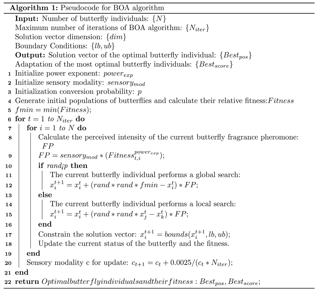
where x j t and x k t denote the j th and k th butterfly individuals in the solution space. Since the fragrance pheromone perceived by the butterfly is limited by many physical conditions, there is a probability factor p in the BOA algorithm that makes the motion behavior of an individual butterfly switch between a global search and a local search. The current paper shows the calculation steps and pseudo-code of the basic butterfly optimization algorithm, The pseudo-code is shown in Algorithm 1.
  • Initialize the number of butterfly individuals ( N ), the number of iterations ( N i t e r ), the transition probabilities of the local and global search ( p ), sensory modality ( c ), power exponent ( a ), solution space dimension ( D i m ), and boundary conditions ( u b , l b ) in the BOA algorithm.
  • The initial butterfly population is randomly generated in the solution space, and the fitness value of each individual is calculated according to the fitness function; the optimal butterfly is found in the initial generation.
  • The perceived intensity generated by the fragrance pheromones of all butterflies is calculated according to the fragrance formula, and the current butterfly movement behavior is determined by the magnitude of the random number r a n d with the transition probability, p .
  • When r a n d < p , the current butterfly performs a global search and migrates to the optimal individual. When r a n d p , then the current butterfly performs local wandering.
  • If the number of iterations of the algorithm reaches the termination condition, the loop ends, and the optimal individual is output. Otherwise, the sensory modality is further updated and returned to step (3), where the sensory modality is updated, as shown in Equation (4):
c t + 1 = c t + 0.025 c t × N i t e r
where c t denotes the value of the sensory modality at the t th iteration.
Drones 06 00393 i001

3.2. BOA-TSAR Algorithm

The butterfly optimization algorithm has superior convergence speed and accuracy compared to other metaheuristics when dealing with simple functions of low dimensionality. However, when the number of dimensions increases with the complexity of the algorithm, the convergence speed and accuracy of the BOA algorithm decrease significantly. Meanwhile, the BOA algorithm has the drawback of local optimal stagnation when dealing with complex multimodal functions, which leads to its slow convergence rate. In order to better solve the above problems, this paper uses Tent chaotic mapping, with the short-period property removed, to optimize the generation distribution of the initial population of the BOA algorithm and improve the BOA algorithm by combining three strategies.

3.2.1. Tent Chaotic Mapping with the Short-Period Property Removed

The BOA algorithm usually uses a randomized approach to generate the initial population of butterflies in the feasible domain, in the process of solving optimization problems. However, the initial solutions generated in this way are prone to an uneven distribution of solution vectors and the phenomenon of distributed aggregation, which makes the algorithm’s optimization search results poor. However, the nonlinearity, sensitive dependence on initial values, ergodicity, and randomness possessed by chaotic sequences can help the BOA algorithm to escape the local optimum more easily during iterative computation and further maintain the diversity of populations.
The Tent chaotic mapping technique has a uniform probability distribution density and good data correlation, and the expression is shown in Equation (5).
x n + 1 = T e n t ( x n ) = x n δ x n [ 0 , δ ) ( 1 x n ) 1 δ x n [ δ , 1 ]
When δ = 0.5 , the Tent chaotic mapping technique has the most typical form, and the resulting sequence of mappings has a uniform distribution that is characterized by a nearly uniform distribution density for different parameters. However, it cannot be ignored that in such cases, the sequences generated by the Tent chaotic mapping technique will have a short-period property to some extent, as shown in Equation (6).
x t = 0.2 x t + 1 = x t δ = 0.4 x t + 2 = x t + 1 δ = 0.8 x t + 3 = 1 x t + 2 1 δ = 0.4 δ = 0.5
Therefore, in this paper, the process of initializing the butterfly population is achieved by adding a small perturbation to the Tent chaotic mapping process to jump out of the period cycle. That is, when x n = x n k and satisfies k ( 1 , 2 , 3 , 4 ) [21], the expression formula of Tent chaotic mapping is shown in Equation (7):
x n + 1 = T e n t ( x n ) = x n + 0.1 3 × frnd ( a , b ) δ x n [ 0 , δ ) 1 ( x n + 0.1 3 × frnd ( a , b ) ) 1 δ x n [ δ , 1 ]
where frnd ( a , b ) is the random number generated by obeying the F distribution. The probability density function of the F distribution shows an asymmetric pattern, i.e., a rapid increase, followed by a slow decrease. This allows the values generated by small perturbations to be distributed over a small interval. This approach breaks the short-period nature of chaotic sequences while maintaining the randomness of the sequence. The probability density formula of the F distribution is shown in Equation (8):
f a , b ( x ) = Γ ( a + b 2 ) Γ ( b 2 ) Γ ( a 2 ) a a 2 b b 2 x a 2 1 ( b + a x ) a + b 2 x > 0 0 x 0
where a is the first degree of freedom and b is the second degree of freedom. After several tests, the random disturbance distribution is more reasonable when a = 3 and b = 5 , as shown in Figure 4.
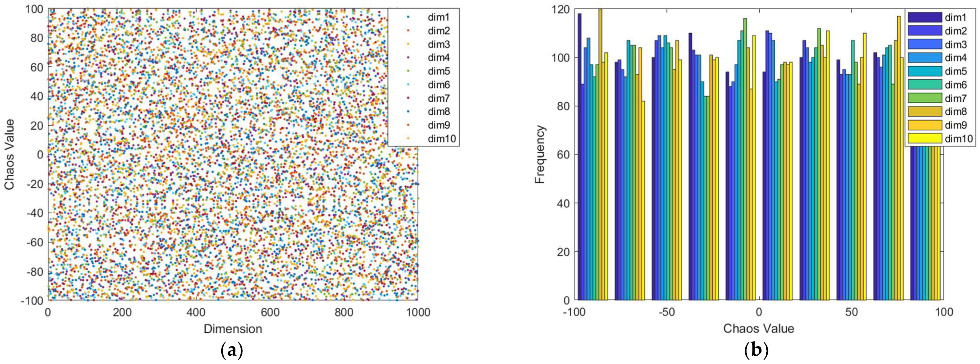
In this paper, 1000 random solution vectors with a dimension of 50 and boundary conditions [−100,100] are generated by the improved Tent chaotic mapping process, and the distribution of the solutions is shown in Figure 5.

3.2.2. Adaptive Nonlinear Inertia Weights

Among metaheuristic algorithms, inertia weights can be used to regulate and control the global exploration and local exploitation capabilities of the algorithm [18]; they also have a crucial impact on the convergence rate of the algorithm. The larger inertia weights give the algorithm better global search capability. The smaller inertia weights are more conducive to the algorithm’s accurate mining in the local area. The inertia weights, based on the linear decreasing strategy proposed by Y. Shi et al., have been widely used due to their simplicity, intuitiveness, and better search performance [22]. However, it is worth noting that reducing the inertia weights linearly in the metaheuristic algorithm leads to a lower convergence rate later in the algorithm and affects the global convergence. At the same time, since the BOA algorithm is, actually, highly nonlinear in its process of searching, this means that the linear decreasing strategy does not accurately reflect the actual algorithmic optimization process.
Therefore, in this paper, in response to the drawbacks of slow convergence speed and the low accuracy of the search results for processing the complex functions that are in the BOA algorithm, adaptive nonlinear inertia weights are introduced in the global search phase of the BOA algorithm, as shown in Equation (9):
ω B O A = ω 1 × ω 2 = 1 ( 1 + F i t n e s s t , g F i t n e s s t , i ) × ( 1 i N i t e r ) 2
where ω B O A denotes the inertia weight value of the current butterfly. F i t n e s s t , g denotes the fitness of the optimal butterfly in the t th iteration. F i t n e s s t , i denotes the fitness of the i th butterfly in the t th iteration. By analyzing Equation (9), it can be seen that the expression of the inertia weight, ω B O A , is divided into two parts; the first half, ω 1 , is related to the fitness of the individual butterfly, and this will automatically be adjusted according to the change in the fitness value of the individual butterfly. The greater the difference between the fitness of the current butterfly individual and the optimal individual, the larger the value of ω 1 , and vice versa, the smaller the value. The second half of the value of ω 2 shows a decreasing trend of deceleration as the number of iterations increases. That is, at the beginning of the algorithm iteration, the value of ω 2 is larger and the global search capability of the algorithm is stronger, which is beneficial for the BOA algorithm when jumping out of the local optimum. As the number of iterations of the algorithm increases, the value of ω 2 gradually becomes smaller; the speed of becoming smaller becomes a gradually decreasing trend, which is conducive to improving the convergence speed and computational accuracy of the BOA algorithm. The improved global search formula of the BOA algorithm is shown in Equation (10).
x i t + 1 = ω B O A × x i t + ( r 2 × g * x i t ) × f i

3.2.3. Simulated Annealing Strategy

The idea of the simulated annealing method was proposed by N. Metropolis et al. in 1953; its starting point was based on the similarity between the annealing process of solid materials and the optimization problem [23]. That is, starting from a certain higher temperature, the global optimal solution of the objective function is found randomly in the solution space as the temperature parameter decreases and combines with the probabilistic sudden-jump property. This simulated annealing method is divided into two parts, namely, the Metropolis acceptance criteria and the material annealing process.
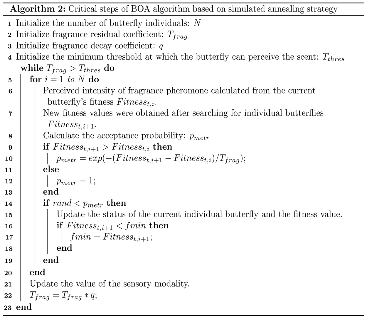
The Metropolis criterion refers to accepting the new state of an individual via probability, rather than using a completely deterministic rule. By using the Metropolis criterion in the BOA algorithm, the inferior individuals can be retained with a certain probability, increasing the diversity of the population, and improving the ability of the BOA algorithm to jump out of the local optimum. The current state of the butterfly individual is assumed to be x i t , and its corresponding fitness is denoted as F i t n e s s t , i . The state of the butterfly after the move is x i + 1 t and the adaptation is F i t n e s s t , i + 1 . Then, the probability of the current butterfly individual’s state, changing from x i t to x i + 1 t , is defined as p m e t r , as shown in Equation (11):
p m e t r = exp ( 1 T f rag ( F i t n e s s t , i + 1 F i t n e s s t , i ) ) F i t n e s s t , i + 1 F i t n e s s t , i 1 F i t n e s s t , i + 1 < F i t n e s s t , i
where T f r a g denotes the fragrance’s residual coefficient in the physical environment, which is reduced by cyclic decay to a threshold that the butterfly cannot perceive and is used as a landmark condition to end the algorithm. The critical pseudo-code based on the simulated annealing strategy is shown in Algorithm 2.
Drones 06 00393 i002

3.2.4. Random Mutation with Global Adaptive Features

In population intelligence algorithms, the diversity and activity of the population play a crucial role in the ergodicity of the algorithm in the solution space. At the initial order of the search performed by the BOA algorithm, proper maintenance of the diversity of the algorithm’s solution vectors helps the algorithm to jump out of the local optimum and prevents the BOA algorithm from reaching premature maturity. The relative reduction in the degree of mutation, as the algorithm converges to come near the global optimal solution and keeps it at a tiny magnitude, can further improve the convergence accuracy of the BOA algorithm without affecting the global convergence rate. Therefore, this paper improves the global search capability of the algorithm by introducing a randomness mutation factor with adaptive features in the global search phase of the BOA algorithm, as shown in Equation (12):
M u = γ 0 + ( 1 2 F i t n e s s t , g π F i t n e s s t , i ) × γ
where γ is the mutation operator and the weight coefficient shows a positive correlation with the difference in fitness between the current butterfly and the optimal butterfly. The γ 0 is the initial mutation operator, and, after several tests, the best expressiveness of the algorithm is achieved when the value of γ 0 is 0.1. The expression of the mutation operator, γ , is shown in Equation (13):
γ = c h i 2 p d f ( χ f r e e ) × ( N i t e r t N i t e r )
where c h i 2 p d f ( χ f r e e ) denotes the chi-square distribution probability density function with a degree of freedom of χ f r e e . It shows a rapidly increasing and then slowly decreasing trend, which helps butterfly individuals to converge to the optimum global position adaptively with the increasing number of iterations. The probability density function of the chi-square distribution is shown in Equation (14):
f k ( x ) = 1 2 χ f r e e 2 Γ ( χ f r e e 2 ) x χ f r e e 2 2 e x 2 ( x > 0 )
where the algorithm is more expressive when χ f r e e = 4 . The global search formula of the BOA algorithm is changed, as shown in Equation (15).
x i t + 1 = x i t + ( r 2 × g * x i t + M u ) × f i

3.2.5. BOA-TSAR Algorithm Flow

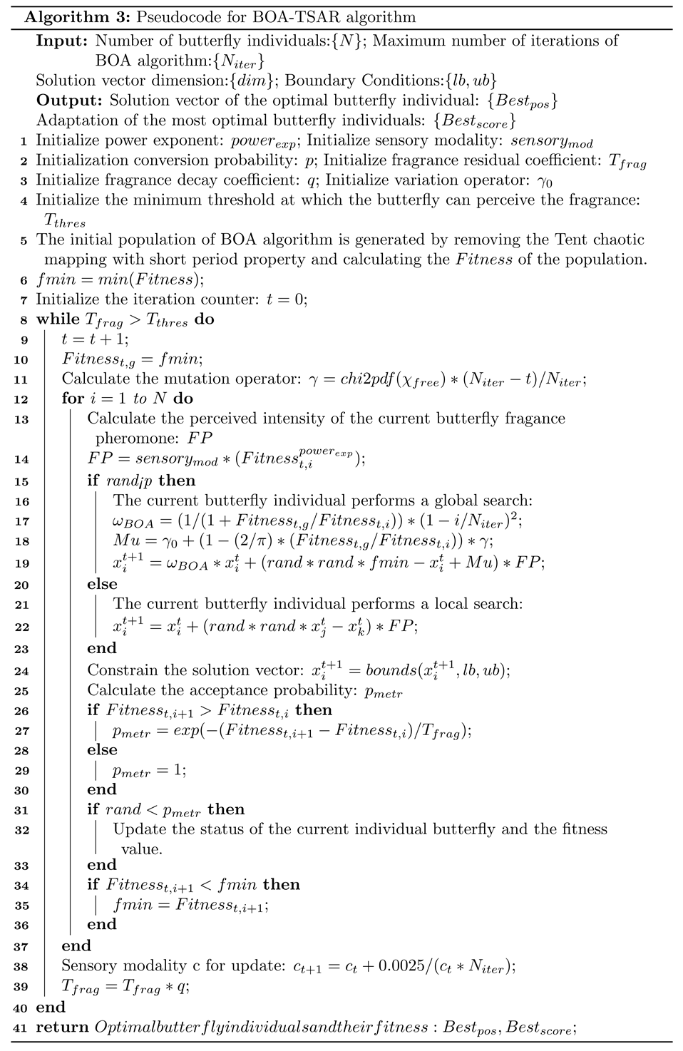
In this paper, we combine the Tent chaotic mapping process with remove short-period properties, nonlinear adaptive inertia weights, a simulated annealing strategy, and a random mutation with global adaptive features to improve the BOA algorithm in terms of the problem of poor convergence speed and the poor accuracy of high-dimensional complex functions, as processed by BOA, and propose the BOA-TSAR algorithm, The pseudo code is shown in Algorithm 3.
Drones 06 00393 i003

4. Drones Path Planning Design Based on BOA-TSAR Algorithm

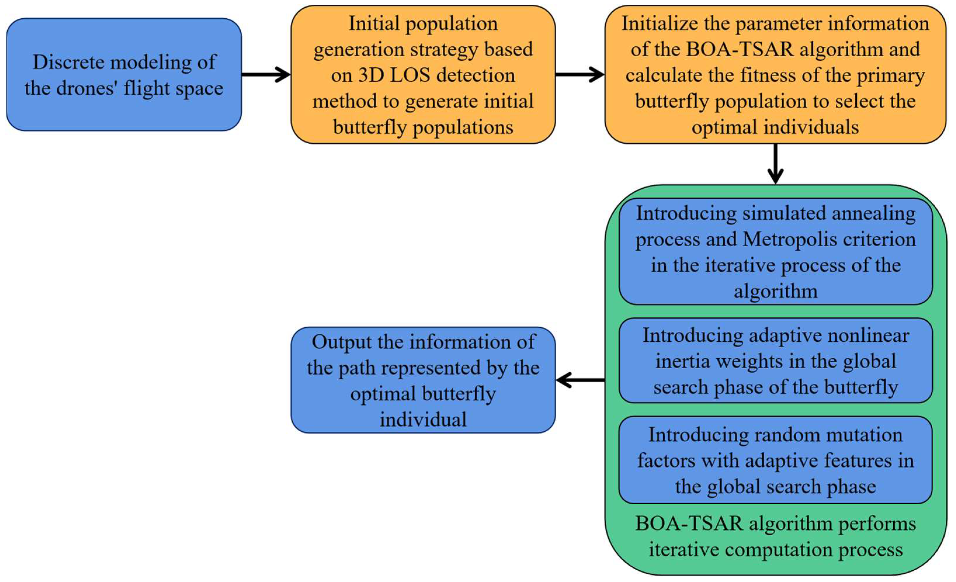
For drones performing near-ground delivery tasks, feasible drone path-planning should take path quality, obstacle avoidance capability, and timeliness into consideration, so as to plan a safe and reliable autonomous obstacle avoidance path under the conditions of ensuring path quality. In this paper, we use the BOA-TSAR algorithm, combined with an improved initial population generation strategy, to achieve the efficient autonomous pathfinding of drones based on a 3D working space; the implementation process is shown in Figure 6.

4.1. Initial Population Generation Strategy Based on 3D LOS Detection Method

In the process of solving drone path-planning using the BOA-TSAR algorithm, the quality of the initial population generation can directly affect the convergence speed and convergence accuracy of the algorithm. The simple use of randomly selected path interruption points will lead to the generation of a large number of infeasible solutions, thus making the diversity of feasible solutions greatly reduced. In the paper [24], the authors propose a discontinuity complementation strategy that uses established rules to achieve complementation for two path nodes that are not adjacent to each other. The paths that are generated in this way will show a large number of useless path interruptions; it will take a great deal of time to check the feasibility of the solution during the search performed by the algorithm, and the time consumption will gradually increase with the expansion of the map size.
In this paper, an initial population generation strategy based on the 3D LOS detection method is proposed to further reduce the generation of path interruption points, while ensuring the diversity of generated feasible solutions via the following steps.
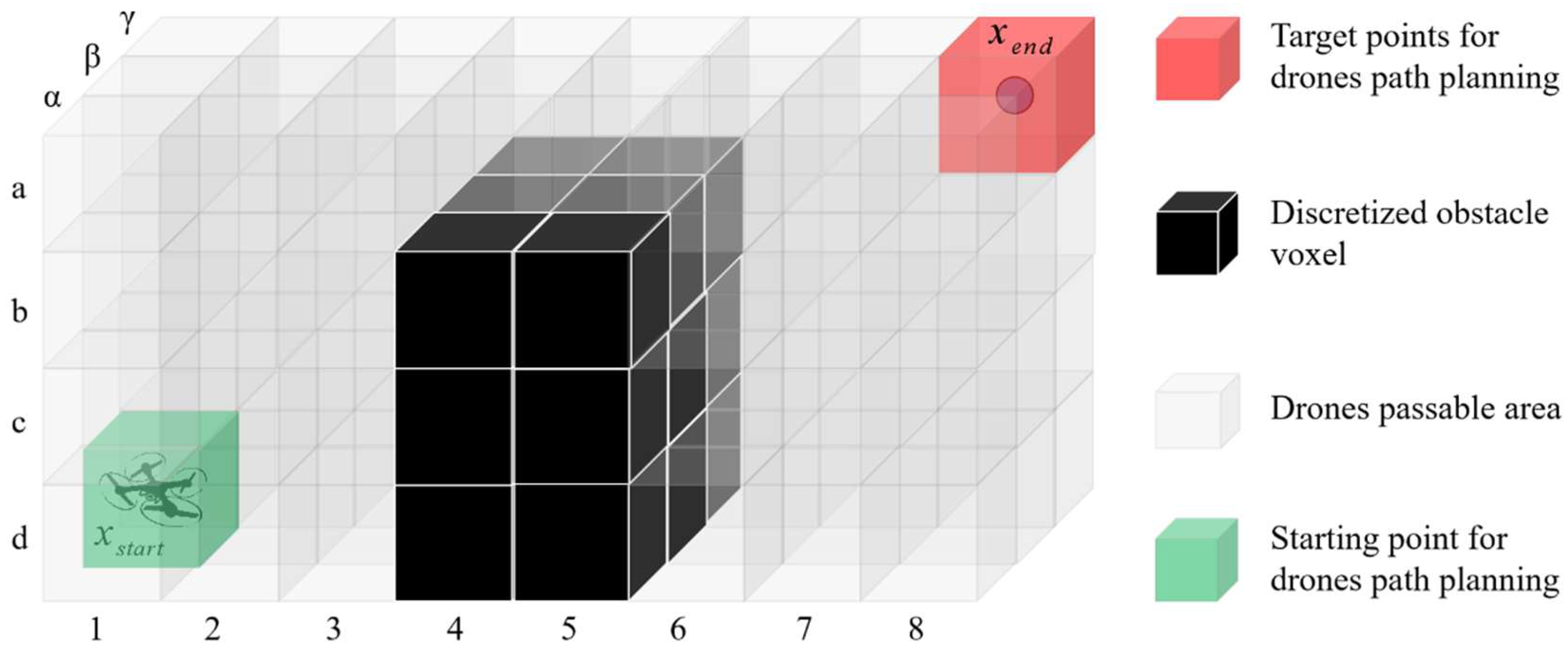
  • Discrete partitioning of the 3D working space of the drones by equal-volume voxels. Considering the safety factor of autonomous flight of the drones, the volume of voxels is set to 1.2 times to 1.5 times the volume of the drones, as shown in Figure 7.
  • To generate feasible path nodes in the discrete drone flight area for the x-axis, y-axis, and z-axis, respectively, using Tent chaotic mapping with short-period removal, and to check the LOS reachability between the generated nodes and their parents and target points.
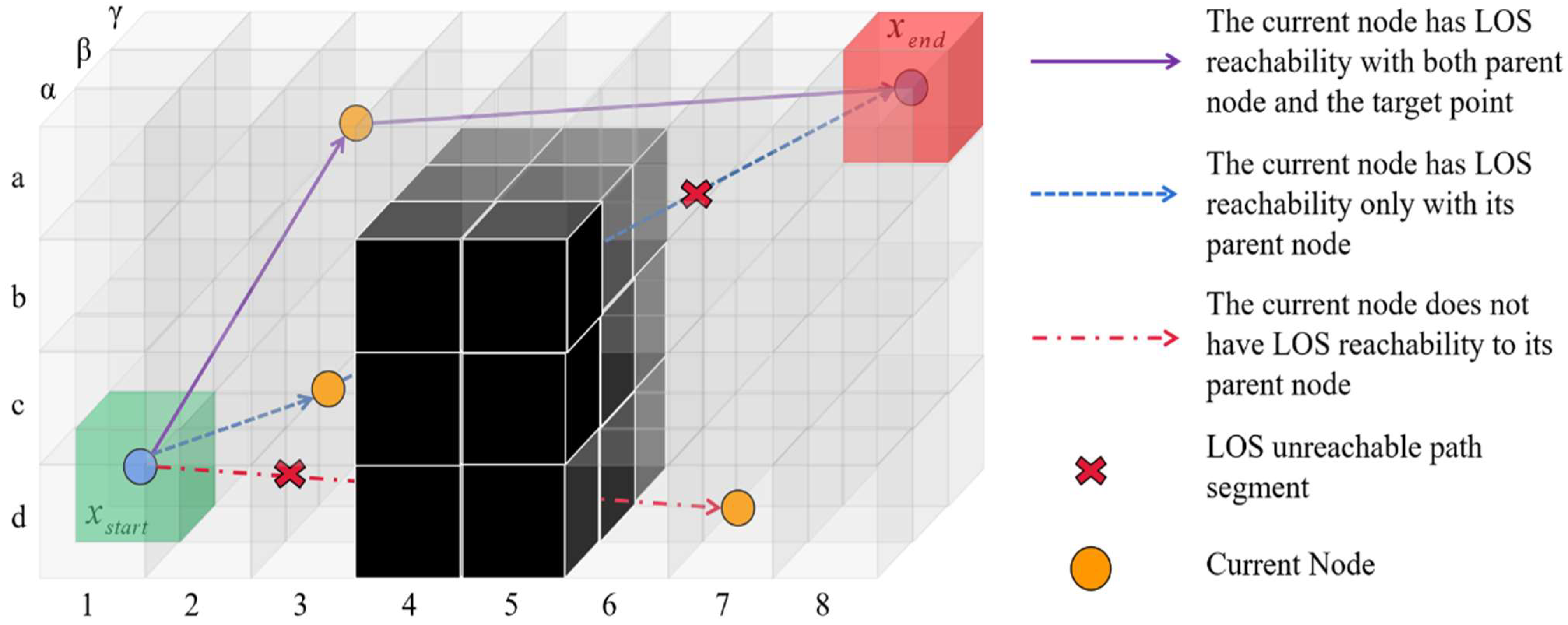
  • If the current node satisfies the LOS reachability requirements with its parent node and target point at the same time, this individual is output, and we return to step (2) for the next butterfly individual generation. If the current node only has LOS reachability with its parent node, the current node is retained as the parent node, and step (2) is continued. If there is no reachability between the current node and its parent node, the current node is discarded directly, as shown in Figure 8.
  • The algorithm generates the initial population in an iterative manner until all the initial butterflies satisfy the feasible solution to end the algorithm.
During the initial population generation, LOS is used as an integral part to detect whether there is direct line-of-sight accessibility between two voxels. LOS detection is often accomplished in two dimensions, using the Bresenham’s line algorithm. The Bresenham’s line algorithm was originally used in image processing to determine the grid of pixels through which a line passes, but it is not applicable in a 3D space [25]. In this paper, the Bresenham’s line algorithm is extended in a 3D space, and the reachability detection between two points of non-equal height is accomplished by using spatial linear equation-based sampling. The In this paper, the implementation steps are given in the form of pseudo-code, as shown in Algorithm 4.
Drones 06 00393 i004

4.2. Mathematical Model for Path Planning

In the path-planning problem model, this paper uses equal-volume voxels to discretize and split the drones’ workspace. Where x s t a r t is defined as the start point of the path, and x e n d is the end point of the path, we set the path interruption point as p k , while the obstacle-free area where the drones can fly is p f r e e . Then, the expression of the path corresponding to butterfly i is shown in Equation (16):
P a t h i = { x s t a r t , p 1 , p 2 , , p k , , p n , x e n d | p k p f r e e } n [ 0 , m a x ( l e n g t h x , l e n g t h y , l e n g t h z ) ]
where m a x ( l e n g t h x , l e n g t h y , l e n g t h z ) indicates the maximum number of voxels in the x-axis, y-axis, and z-axis of the workspace.
During the iterative computation of the algorithm, the fitness function of path planning is used to calculate the cost required to generate a path, while the magnitude of the fitness function is used to determine the quality of the generated path. The fitness function established in this paper is shown in Equation (17):
F i t n e s s ( p a t h i ) = ψ 1 F 1 ( p a t h i ) + ψ 2 F 2 ( p a t h i )
where F i t n e s s ( p a t h i ) denotes the fitness of the path corresponding to the butterfly individual, i . F 1 and F 2 denote the cost functions needed to calculate the fitness. ψ 1 and ψ 2 denote the current values of the weights that the two cost functions have and that satisfy Equation (18).
i = 1 2 ψ i = 1 , ψ i 0
In order to ensure the safety and efficiency of the drone during the autonomous mission, the total distance of the path generated by the BOA-TSAR algorithm and the total turning angle of the path are considered comprehensively in this paper. In the process of adaptation calculation, F 1 ( p a t h i ) denotes the distance cost required to generate the path, which is calculated in this paper using the 3D Euclidean distance method, the expression of which is shown in Equation (19).
F 1 ( p a t h i ) = ( x s t a r t . x p 1 . x ) 2 + ( x s t a r t . y p 1 . y ) 2 + ( x s t a r t . z p 1 . z ) 2 + k = 1 n 1 ( p k + 1 . x p k . x ) 2 + ( p k + 1 . y p k . y ) 2 + ( p k + 1 . z p k . z ) 2 + ( p n . x x e n d . x ) 2 + ( p n . y x e n d . y ) 2 + ( p n . z x e n d . z ) 2
F 2 ( p a t h i ) denotes the total turning angle of the path generated by the BOA-TSAR algorithm, as shown in Equation (20):
F 2 ( p a t h i ) = i = 1 n 1 r a d 2 d e g ( a c o s ( V i V i + 1 | V i | | V i + 1 | ) )
where V i denotes the vector difference composed by the path nodes. The complete path of the drone search is illustrated in Figure 9.

5. Experiment and Simulation

In the algorithm experiments, as well as the simulation part, to verify the effectiveness of the proposed BOA-TSAR algorithm, 24 CEC benchmark functions from different years were selected for algorithm testing in this paper, the details of which can be found in articles [15,16,26], as shown in Table 1, which shows the names, expressions, variable dimensions, and minimum values of each benchmark test function. In this paper, three sets of experiments will be conducted for the BOA-TSAR algorithm, based on the MATLAB 2020b simulation software on an i5-1135G7 minicomputer; the specific experimental design is as follows.
  • In order to better validate the improved strategy proposed in this paper and the actual operation capability of the algorithm, benchmark function tests were conducted for the original BOA algorithm, the BOA-TSAR algorithm, and the three sub-algorithms of the improved version. The three sub-algorithms are the BOA algorithm, based on a simulated annealing strategy (BOA-SA), a BOA algorithm based on adaptive nonlinear inertia weights (BOA-AIW), and a BOA algorithm based on the random mutation of global adaptive features (BOA-RV). In terms of experimental design, the benchmark functions are selected as six unimodal and six multimodal functions, which are tested in the dimension of Dim = 50 and Dim = 100, respectively, so as to verify the effectiveness of the improvement strategy that is proposed in this paper.
  • To further analyze the performance of the algorithm proposed in this paper and to produce satisfactory results when dealing with optimization problems, in this paper, four mainstream population intelligence search algorithms that are often used to solve complex optimization problems, namely, the genetic algorithm (GA) [27,28,29], particle swarm optimization (PSO) algorithm [30,31], gray wolf optimization (GWO) algorithm [32,33], and the artificial bee colony (ABC) algorithm [34], based on 24 benchmark functions, are selected for cross-sectional comparison tests.
  • This paper conducts drone 3D path-planning experiments, based on the public map dataset of Moving AI Lab. This experiment uses six 3D maps of different cities to conduct comparison tests against the BOA-TSAR algorithm, the A-Star algorithm [35,36,37], the Jump Point Search (JPS) algorithm [38,39,40], the RRT algorithm [41], and the Theta* algorithm [42], as proposed in this paper.

5.1. Experiment 1

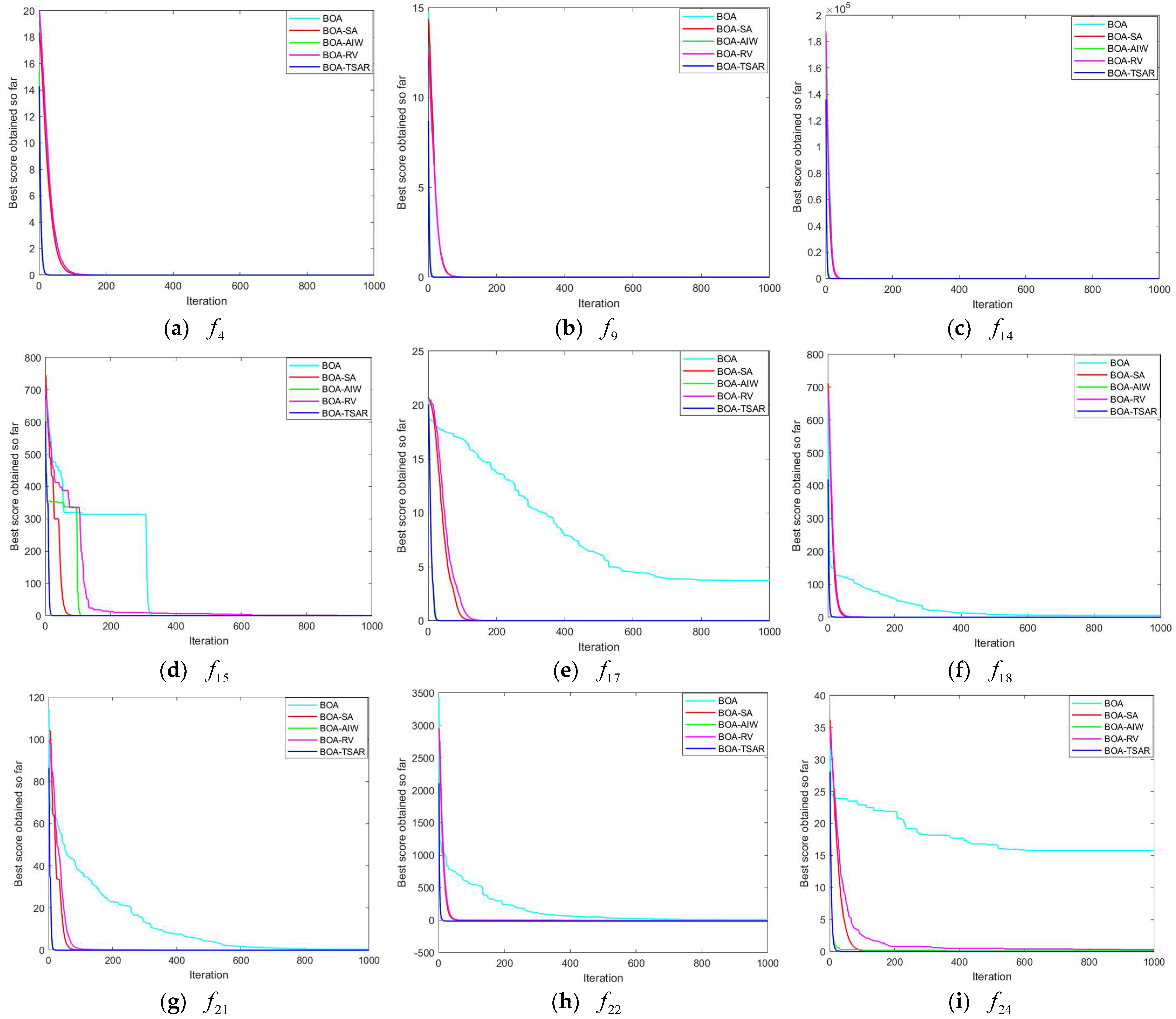
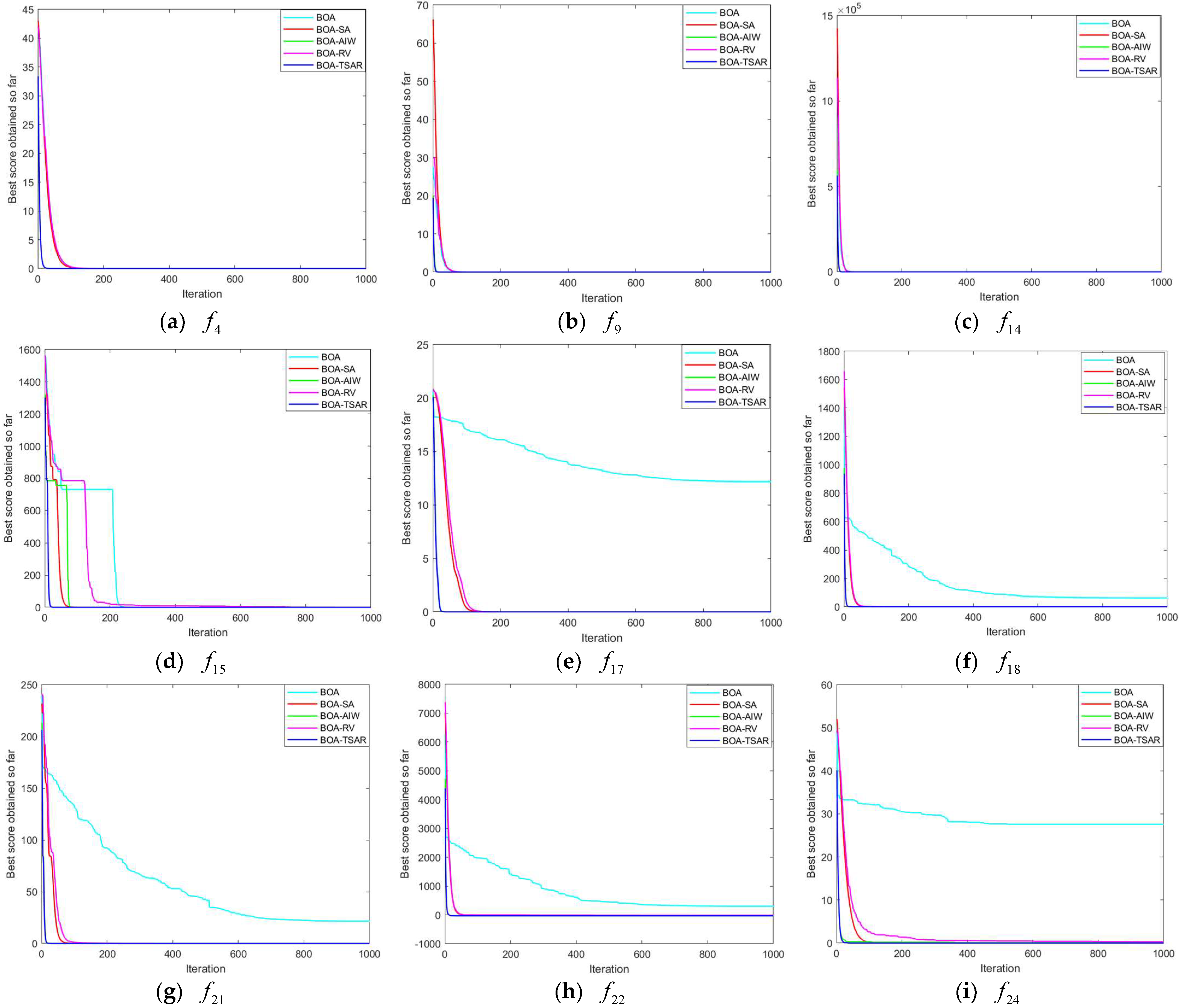
In this experiment, six unimodal functions ( f 1 , f 3 , f 4 , f 6 , f 9 , and f 14 ) and six multimodal functions ( f 15 , f 17 , f 18 , f 21 , f 22 , and f 24 ) are selected from Table 1 for the BOA algorithm, the BOA-TSAR algorithm, and the three modified sub-algorithms in the dimension of Dim = 50 and Dim = 100. The initial populations of all algorithms in the experimental procedure are generated using the modified Tent chaotic mapping. The initial number of individuals is set to 200 and the maximum number of iterations is set to 1000. Due to the small variability of the test results for the unimodal functions, only a partial display is made here, as shown in Figure 10 and Figure 11. The rest of the experimental results are shown in Figure A1 and Figure A2 in Appendix A.
In the comparison experiments in two different dimensions, it can be seen that the convergence speed of the five algorithms shows less difference for the test case of the unimodal functions. The BOA-TSAR algorithm has the best expressiveness and the fastest convergence under f 1 , f 3 , f 6 , f 9 , and f 14 for Dim = 50, while BOA-AIW has the best expressiveness in f 4 . BOA-SA and BOA-RV converge at about the same rate as the BOA algorithm. The BOA-TSAR algorithm still converges fastest under f 1 , f 3 , f 6 , f 9 and f 14 for Dim = 100, but the convergence speed of BOA-SA and BOA-RV is similar to that of the original BOA algorithm and weaker than that of the original BOA algorithm under f 4 , f 6 , and f 9 . In the test of the multimodal functions, the difference in the convergence speed of each algorithm is large. In the tests with Dim = 50 and Dim = 100, the convergence speed of BOA-TSAR algorithm is the fastest, and the local stagnation of the original BOA algorithm is greatly weakened under f 15 and f 21 . Among all the improved sub-algorithms, BOA-AIW has the best expressiveness in terms of convergence speed and is more effective in improving the local stagnation phenomenon. The performance of BOA-RV is weaker, and the convergence speed is worse compared with other improved algorithms. The average (Avg) and standard deviation (Std) of the adaptation after 30 runs for each benchmark function in the experiment are shown in Table 2 and Table 3.
From Table 2 and Table 3, it can be seen that the convergence accuracy of all five algorithms in the testing process of unimodal functions ( f 1 , f 3 , f 4 , f 6 , f 9 , f 14 ) is relatively good. Among them, the BOA-TSAR algorithm has the highest convergence accuracy among all unimodal functions, and the convergence accuracy of the BOA-SA algorithm and the BOA-RV algorithm is more similar to the test results of the original BOA algorithm. In the multimodal functions ( f 15 , f 17 , f 18 , f 21 , f 22 , f 24 ) test results, the convergence of the BOA algorithm is not ideal, where the convergence of the BOA algorithm during the f 17 , f 18 , f 24 test differs significantly from the theoretical optimum. The BOA-TSAR algorithm proposed in this paper has the best performance and the highest convergence accuracy in the multimodal functions test. In this experiment, the BOA-TSAR algorithm shows superior performance and finds theoretical optimal values for all complex functions in low- and high-dimensional conditions.

5.2. Experiment 2

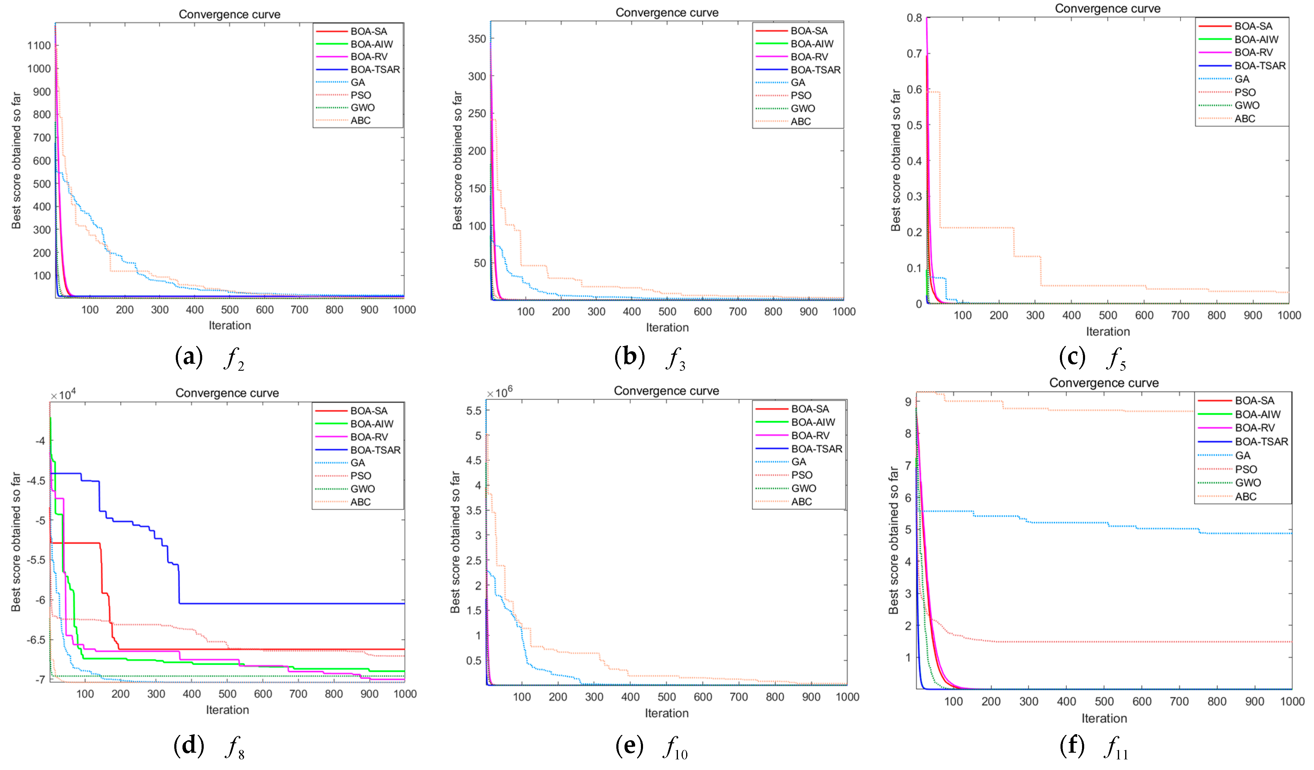
In this experiment, BOA-SA, BOA-AIW, BOA-RV, BOA-TSAR, GA, PSO, GWO, and ABC are selected for cross-sectional comparison tests, based on the 24 benchmark functions listed in this paper in the Dim = 50 dimension. The test results are presented as the average (Avg) and standard deviation (Std) of the results of 30 experiments. The parameter settings of the algorithms involved in the comparison experiments are shown in Table 4, where p c denotes the crossover probability of the GA algorithm and p m denotes the variance probability. c 1 and c 2 denote the learning factors of the PSO algorithm, and ω M a x and ω M i n denote the maximum and minimum values of the inertia weights. T l i m i t denotes the maximum number of update-free iterations of the ABC algorithm for the detection bee solution, S N denotes the number of food sources, and D denotes the problem dimension. The parameters concerning the improved BOA algorithm have been described in the text. The convergence curves of some of the experiments are shown in Figure 12.
From the convergence graphs, we can see that the convergence speed and the ability to jump out of the local optimum of the BOA-TSAR algorithm are excellent compared to other algorithms. Except in the case of f 8 and f 16 , the BOA-TSAR algorithm converges to the theoretical optimum faster, compared to the other seven algorithms. From f 5 , f 15 , and f 16 , the ABC algorithm has the most obvious local optimal point-stagnation phenomenon, and the stepwise convergence method leads to a decrease in its convergence speed and accuracy, and the convergence result differs greatly from the theoretical optimal value. From the test results of f 8 , the GWO algorithm has the fastest convergence speed and BOA-VR has the highest convergence accuracy. The adaptive random mutation, based on the chi-square distribution probability density function used in BOA-VR, enhances the randomness of the butterfly’s search in the overall space, to a certain extent, which is beneficial for improving the convergence accuracy of the algorithm in the late iteration of the algorithm. In the tests of f 11 , f 15 , f 17 and f 20 , we can see that the convergence of GA, PSO and ABC is poor, and the phenomenon of falling into a local optimum and not being able to escape is more obvious, while conversely, the performance of other algorithms is better. In the test results of f 16 , we can see that the iterative results of the GA algorithm are closest to the theoretical optimum, and the convergence accuracy of PSO and BOA-TSAR are more similar, but still show a gap with the theoretical optimum. The convergence results of each algorithm are shown in Table 5.
From the convergence results of each algorithm, the BOA-TSAR algorithm and its improved sub-algorithms converge to the theoretical optimum for all benchmark function tests except f 8 , f 10 , and f 16 , especially BOA-TSAR, the convergence accuracy of which is much higher than the other algorithms. The convergence accuracy of GA and ABC in the testing process is poor, except for f 5 and f 6 ; the convergence results of the rest of the tested functions have a large gap with the theoretical optimal value, where it is easy to fall into the local optimum. The GWO algorithm also performs better in the test results, where the convergence accuracy of f 1 to f 7 , and f 9 to f 14 , f 17 , and f 19 to f 21 are better than BOA-SA and BOA-RV. GWO shows better convergence accuracy than BOA-AIW in the tests of f 19 and f 20 . In the cross-sectional comparison of the convergence experiments of the benchmark functions of the eight algorithms, it is easy to see that the BOA-TSAR algorithm has superior solving ability in the face of complex functions and can find the theoretical optimal value under most of the complex functions. These results indicate that the improved strategy proposed in this paper has helped the BOA algorithm well in solving the problems of slow convergence and low accuracy under high-dimensional complex functions. At the same time, the BOA-TSAR algorithm shows a strong competitiveness among the same types of population intelligence algorithms. To get a clearer picture of the final results of the comparison experiments, we will rank each algorithm according to its performance in the Wilcoxon rank test and give the tied rank of each algorithm, as shown in Table 6. It is worth noting that when the results of two algorithms are the same, the tied rank will take an equalization strategy for ranking (see article [17] for a similar analysis).
As can be seen in Table 6, the BOA-TSAR algorithm obtained the 20 best ranks among the 24 sets of benchmark functions tested, with excellent convergence accuracy. The BOA-AIW algorithm is the second most effective choice, followed by GWO, BOA-SA, BOA-VR, PSO, GA, and ABC. The ranking results support the previous experimental analysis and the conclusion of this paper that the BOA-TSAR algorithm shows the best convergence speed and convergence accuracy in the comparison experiments.

5.3. Experiment 3

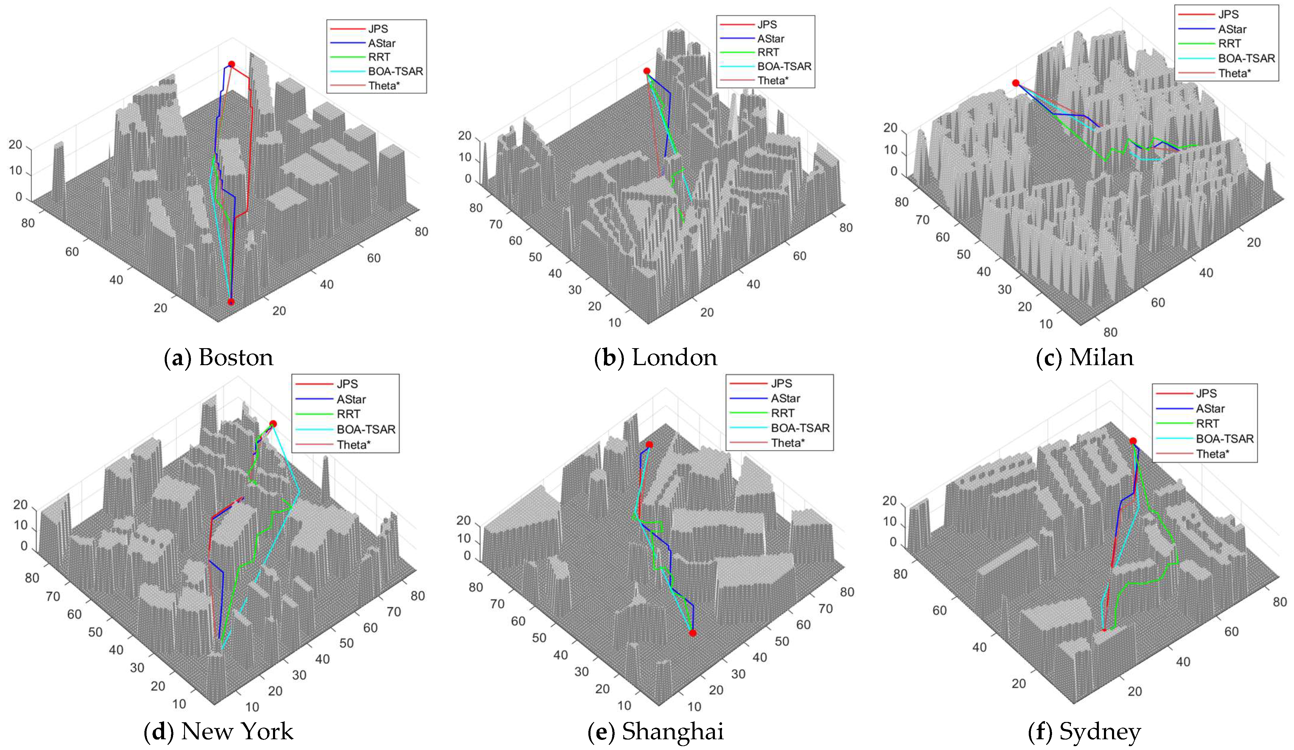
In the drone path-planning experiments, six city maps taken from Moving AI Lab’s 3D public map dataset are used for the algorithm comparison tests. The selection of one of the maps is shown in Figure 13. In the test, the A-Star and JPS algorithms, based on graph search technology, the RRT algorithm, based on sampling technology, and the Theta* algorithm, based on multi-angle pathfinding technology were selected for lateral comparative experiments among the various drone pathfinding technologies. According to the principle of fairness, the A-Star algorithm and JPS algorithm both use the Euclidean distance formula as the heuristic function. The search step of the RRT algorithm is set to 1 voxel length (the distance from the center of one voxel to the center of another voxel), while the tree node collision detection of RRT uses the same 3D LOS detection method as in the initial butterfly generation strategy of BOA-TSAR. In the testing process, five algorithms perform 3D path planning, using the same starting point and target point. The path-planning results will compare the time complexity, space occupation size, the total length of the generated paths, the path smoothness metric, and the number of path nodes of each algorithm, where the path smoothness metric is defined as the total turning angle of the path generated by the algorithm. The experimental simulation results are shown in Figure 14, below.
From the test results shown in Figure 13, it can be seen that all five path-planning algorithms can complete the pathfinding in the drones’ 3D workspace. Among them, the RRT algorithm generates paths very rapidly, but the path results that it obtains are poor. Although the path obtained by the RRT algorithm does not appear to collide with obstacles, the path nodes are generated by sampling, which leads to high randomness of the path direction and poor path generation. The A-Star algorithm and the JPS algorithm often obtain the shortest resulting path under discrete voxels during the pathfinding process. However, it is worth noting that the paths obtained by A-Star and JPS still differ from the actual optimum due to the restrictive nature of their search directions. The Theta* algorithm, based on the multi-angle pathfinding technique, performs well among the six experiments, and the resultant paths obtained are closer to the actual optimum because they are no longer restricted by the search direction; however, the large number of angle transferability calculations also leads to high time complexity and space complexity of the Theta* algorithm. Since the BOA-TSAR algorithm incorporates an improved initial population generation strategy that greatly reduces the generation of unnecessary path interruptions, the BOA-TSAR algorithm has the smallest number of nodes among all experiments and also has the fewest turn angles and smoother paths. In this paper, the experimental results are presented, as shown in Table 7.
Analyzing the generated path lengths of the five algorithms, the BOA-TSAR algorithm obtained the shortest paths in all four sets of comparison experiments, except for the map test in Boston and Sydney, where the path lengths were longer than those generated by the Theta* algorithm. Meanwhile, the path generated by the BOA-TSAR algorithm has the smallest total turning angle among the six groups of comparison experiments, and the resulting path is smoother than with other algorithms. In terms of the time complexity and space complexity of the algorithm, the BOA-TSAR algorithm requires a longer running time and occupies more space than the A-Star and JPS algorithms. However, the time complexity and space complexity of the BOA-TSAR algorithm are lower than those of the Theta* algorithm in the case of a better quality of generated paths.
6. Conclusions

For drones performing near-ground delivery missions, the autonomous navigation of the drones will be the decisive factor in mission success. Path-planning for the 3D working space of drones has received more and more attention as a key technology for autonomous navigation. Under the premise of ensuring safety, a shorter and smoother path will undoubtedly significantly reduce the time for drones to perform their tasks and improve their efficiency. Based on the above problems, this paper will realize the path-planning design of drones using the modified BOA algorithm to achieve the safe delivery of drones in complex low-altitude environments. The work of this paper can be summarized as follows.
  • In order to avoid the generation of a distributed aggregation of populations due to random numbers, this paper replaces the randomness strategy in the initial butterfly generation process of the BOA algorithm by using Tent chaotic mapping. At the same time, the generated sequence of Tent chaotic mapping is avoided to have a short-period property by a small perturbation, based on the F distribution.
  • In this paper, the BOA-TSAR algorithm is proposed via adaptive nonlinear inertia weights, a simulated annealing strategy, and random mutation with global adaptive features. The BOA-TSAR algorithm improves the drawbacks of slow convergence, low accuracy, and local optimal stagnation to achieve the complex functions that exist in the BOA algorithm. As can be seen from Experiment 5.1, the BOA-TSAR algorithm showed the best convergence speed and convergence accuracy during the testing of unimodal and multimodal functions. At the same time, the BOA-TSAR algorithm also showed strong competitiveness among similar group-intelligence algorithms in the cross-sectional comparative experiments detailed in Experiment 5.2.
  • Based on the BOA-TSAR algorithm in path-planning design, the initial butterfly has the problem of redundant nodes. In this paper, an initial population generation strategy based on the 3D LOS detection method is proposed, to further reduce the generation of path interruption points, while ensuring the diversity of generated feasible solutions. The cross-sectional comparability tests, based on publicly available datasets, show that the 3D paths generated by the BOA-TSAR algorithm perform well in terms of path length and path smoothness metrics. However, the BOA-TSAR algorithm also has the following problems; from the test results, we can see that the time complexity and space complexity of the BOA-TSAR algorithm are still high.
In terms of future work, we need to further reduce the time complexity and space complexity of the BOA-TSAR algorithm. It is also necessary to study the dynamic obstacles that occur in the drone’s near-ground flight and realize the autonomous navigation of the drones in the dynamic environment.

Author Contributions

Data curation, Q.Q. and L.H.; Investigation, Q.Q. and Y.L. (Yanyu Liu); Resources, Y.L. (Yuan Luo) and Y.Z.; Software, J.L. and K.Z.; Supervision, Y.Z.; Writing—original draft, J.L.; Writing—review & editing, J.L. All authors have read and agreed to the published version of the manuscript.

Funding

This research was funded by Research Project of China Disabled Persons’ Federation on assistive technology: 2022CDPFAT-01.

Institutional Review Board Statement

Not applicable.

Informed Consent Statement

Not applicable.

Data Availability Statement

Publicly available datasets were analyzed in this study. This data can be found here: [https://movingai.com/].

Conflicts of Interest

The authors declare no conflict of interest.

Appendix A

Figure A1. Comparison of convergence curves between BOA, BOA-SA, BOA-AIW, BOA-RV, and BOA-TSAR for unimodal functions of f 1 , f 3 , and f 6 at Dim = 50.
Drones 06 00393 g0a1
Figure A2. Comparison of convergence curves between BOA, BOA-SA, BOA-AIW, BOA-RV, and BOA-TSAR for unimodal functions of f 1 , f 3 , and f 6 at Dim = 100.
Drones 06 00393 g0a2

References

  1. Adão, T.; Hruška, J.; Pádua, L.; Bessa, J.; Peres, E.; Morais, R.; Sousa, J.J. Hyperspectral imaging: A review on UAV-based sensors, data processing and applications for agriculture and forestry. Remote Sens. 2017, 9, 1110. [Google Scholar] [CrossRef] [Green Version]
  2. Klosterman, S.; Melaas, E.; Wang, J.A.; Martinez, A.; Frederick, S.; O’Keefe, J.; Orwig, D.A.; Wang, Z.; Sun, Q.; Schaaf, C. Fine-scale perspectives on landscape phenology from unmanned aerial vehicle (UAV) photography. Agric. For. Meteorol. 2018, 248, 397–407. [Google Scholar] [CrossRef]
  3. Menouar, H.; Guvenc, I.; Akkaya, K.; Uluagac, A.S.; Kadri, A.; Tuncer, A. UAV-enabled intelligent transportation systems for the smart city: Applications and challenges. IEEE Commun. Mag. 2017, 55, 22–28. [Google Scholar] [CrossRef]
  4. Everaerts, J. The use of unmanned aerial vehicles (UAVs) for remote sensing and mapping. Int. Arch. Photogramm. Remote Sens. Spat. Inf. Sci. 2008, 37, 1187–1192. [Google Scholar]
  5. Scherer, J.; Yahyanejad, S.; Hayat, S.; Yanmaz, E.; Andre, T.; Khan, A.; Vukadinovic, V.; Bettstetter, C.; Hellwagner, H.; Rinner, B. An autonomous multi-UAV system for search and rescue. In Proceedings of the First Workshop on Micro Aerial Vehicle Networks, Systems, and Applications for Civilian Use, Florence, Italy, 18 May 2015; pp. 33–38. [Google Scholar]
  6. Goerzen, C.; Kong, Z.; Mettler, B. A survey of motion planning algorithms from the perspective of autonomous UAV guidance. J. Intell. Robot. Syst. 2010, 57, 65–100. [Google Scholar] [CrossRef]
  7. Yang, L.; Qi, J.; Xiao, J.; Yong, X. A literature review of UAV 3D path planning. In Proceedings of the 11th World Congress on Intelligent Control and Automation, Shenyang, China, 29 June–4 July 2014; pp. 2376–2381. [Google Scholar]
  8. Ezugwu, A.E.; Shukla, A.K.; Nath, R.; Akinyelu, A.A.; Agushaka, J.O.; Chiroma, H.; Muhuri, P.K. Metaheuristics: A comprehensive overview and classification along with bibliometric analysis. Artif. Intell. Rev. 2021, 54, 4237–4316. [Google Scholar] [CrossRef]
  9. Del Ser, J.; Osaba, E.; Molina, D.; Yang, X.-S.; Salcedo-Sanz, S.; Camacho, D.; Das, S.; Suganthan, P.N.; Coello, C.A.C.; Herrera, F. Bio-inspired computation: Where we stand and what’s next. Swarm Evol. Comput. 2019, 48, 220–250. [Google Scholar] [CrossRef]
  10. Zhang, N.; Zhang, M.; Low, K.H. 3D path planning and real-time collision resolution of multirotor drone operations in complex urban low-altitude airspace. Transp. Res. Part C Emerg. Technol. 2021, 129, 103123. [Google Scholar] [CrossRef]
  11. Faria, M.; Maza, I.; Viguria, A. Applying frontier cells based exploration and Lazy Theta* path planning over single grid-based world representation for autonomous inspection of large 3D structures with an UAS. J. Intell. Robot. Syst. 2019, 93, 113–133. [Google Scholar] [CrossRef] [Green Version]
  12. Lin, X.; Wang, C.; Wang, K.; Li, M.; Yu, X. Trajectory planning for unmanned aerial vehicles in complicated urban environments: A control network approach. Transp. Res. Part C Emerg. Technol. 2021, 128, 103120. [Google Scholar] [CrossRef]
  13. Meng, L.; Qing, S.; Jun, Z.Q. UAV path re-planning based on improved bidirectional RRT algorithm in dynamic environment. In Proceedings of the 2017 3rd International Conference on Control, Automation and Robotics (ICCAR), Nagoya, Japan, 22–24 April 2017; pp. 658–661. [Google Scholar]
  14. Wang, J.; Chi, W.; Li, C.; Wang, C.; Meng, M.Q.-H. Neural RRT*: Learning-based optimal path planning. IEEE Trans. Autom. Sci. Eng. 2020, 17, 1748–1758. [Google Scholar] [CrossRef]
  15. Wang, X.; Pan, J.-S.; Yang, Q.; Kong, L.; Snášel, V.; Chu, S.-C. Modified Mayfly Algorithm for UAV Path Planning. Drones 2022, 6, 134. [Google Scholar] [CrossRef]
  16. Wang, Y.; Bai, P.; Liang, X.; Wang, W.; Zhang, J.; Fu, Q. Reconnaissance mission conducted by UAV swarms based on distributed PSO path planning algorithms. IEEE Access 2019, 7, 105086–105099. [Google Scholar] [CrossRef]
  17. Arora, S.; Singh, S. Butterfly optimization algorithm: A novel approach for global optimization. Soft Comput. 2019, 23, 715–734. [Google Scholar] [CrossRef]
  18. Liu, J.-S.; Ma, Y.-X.; Li, Y. Improved Butterfly Algorithm for Multi-dimensional Complex Function Optimization Problem. Tien Tzu Hsueh Pao/Acta Electron. Sin. 2021, 49, 1068–1076. [Google Scholar] [CrossRef]
  19. Tubishat, M.; Alswaitti, M.; Mirjalili, S.; Al-Garadi, M.A.; Alrashdan, M.T.; Rana, T.A. Dynamic Butterfly Optimization Algorithm for Feature Selection. IEEE Access 2020, 8, 194303–194314. [Google Scholar] [CrossRef]
  20. Zhou, H.; Zhang, G.; Wang, X.; Ni, P.; Zhang, J. Structural identification using improved butterfly optimization algorithm with adaptive sampling test and search space reduction method. Structures 2021, 33, 2121–2139. [Google Scholar] [CrossRef]
  21. Zhou, P.; Dong, C.-Y.; Chen, X.-Y.; Qi, Y.-S.; Zhao, X.-Y.; Wang, Q.-L. A Salp Swarm Algorithm Based on Stepped Tent Chaos and Simulated Annealing. Tien Tzu Hsueh Pao Acta Electron. Sin. 2021, 49, 1724–1735. [Google Scholar] [CrossRef]
  22. Shi, Y.; Eberhart, R. A modified particle swarm optimizer. In Proceedings of the 1998 IEEE international conference on evolutionary computation proceedings. IEEE world congress on computational intelligence (Cat. No. 98TH8360), Anchorage, AK, USA, 4–9 May 1998; pp. 69–73. [Google Scholar]
  23. Metropolis, N.; Rosenbluth, A.W.; Rosenbluth, M.N.; Teller, A.H.; Teller, E. Equation of state calculations by fast computing machines. J. Chem. Phys. 1953, 21, 1087–1092. [Google Scholar] [CrossRef] [Green Version]
  24. Liu, Z.; Xue, Y.; Zhou, C.; Bai, H.; Cui, X. Population Initialization Improvement of Robot Path Planning Based on Genetic Algorithm. Mach. Tool Hydraul. 2021, 47, 5–8. [Google Scholar]
  25. Luo, Y.; Lu, J.; Zhang, Y.; Qin, Q.; Liu, Y. 3D JPS Path Optimization Algorithm and Dynamic-Obstacle Avoidance Design Based on Near-Ground Search Drone. Appl. Sci. 2022, 12, 7333. [Google Scholar] [CrossRef]
  26. Jia, H.; Wei, Z.; He, X.; Zhang, L.; He, J.; Mu, Z. Path Planning Based on Improved Particle Swarm Optimization Algorithm. Nongye Jixie Xuebao Trans. Chin. Soc. Agric. Mach. 2018, 49, 371–377. [Google Scholar] [CrossRef]
  27. Mirjalili, S. Genetic algorithm. In Evolutionary Algorithms and Neural Networks; Springer: Berlin/Heidelberg, Germany, 2019; pp. 43–55. [Google Scholar]
  28. Han, S.; Xiao, L. An improved adaptive genetic algorithm. In Proceedings of the SHS Web of Conferences, Nicosia/TRNC, Cyprus, 22–25 September 2022; p. 01044. [Google Scholar]
  29. Deng, W.; Zhang, X.; Zhou, Y.; Liu, Y.; Zhou, X.; Chen, H.; Zhao, H. An enhanced fast non-dominated solution sorting genetic algorithm for multi-objective problems. Inf. Sci. 2022, 585, 441–453. [Google Scholar] [CrossRef]
  30. Zhang, Y.; Gong, D.-w.; Zhang, J.-h. Robot path planning in uncertain environment using multi-objective particle swarm optimization. Neurocomputing 2013, 103, 172–185. [Google Scholar] [CrossRef]
  31. Li, G.; Chou, W. Path planning for mobile robot using self-adaptive learning particle swarm optimization. Sci. China Inf. Sci. 2018, 61, 052204. [Google Scholar] [CrossRef] [Green Version]
  32. Jamshidi, V.; Nekoukar, V.; Refan, M.H. Real time UAV path planning by parallel grey wolf optimization with align coefficient on CAN bus. Clust. Comput. 2021, 24, 2495–2509. [Google Scholar] [CrossRef]
  33. Liu, Y.; Li, X. A Hybrid Mobile Robot Path Planning Scheme Based on Modified Gray Wolf Optimization and Situation Assessment. J. Robot. 2022, 2022, 4167170. [Google Scholar] [CrossRef]
  34. Bhattacharjee, P.; Rakshit, P.; Goswami, I.; Konar, A.; Nagar, A.K. Multi-robot path-planning using artificial bee colony optimization algorithm. In Proceedings of the 2011 Third World Congress on Nature and Biologically Inspired Computing, Salamanca, Spain, 19–21 October 2011; pp. 219–224. [Google Scholar]
  35. Duchoň, F.; Babinec, A.; Kajan, M.; Beňo, P.; Florek, M.; Fico, T.; Jurišica, L. Path planning with modified A-Star algorithm for a mobile robot. Procedia Eng. 2014, 96, 59–69. [Google Scholar] [CrossRef] [Green Version]
  36. Tang, G.; Tang, C.; Claramunt, C.; Hu, X.; Zhou, P. Geometric A-star algorithm: An improved A-star algorithm for AGV path planning in a port environment. IEEE Access 2021, 9, 59196–59210. [Google Scholar] [CrossRef]
  37. Wang, C.; Wang, L.; Qin, J.; Wu, Z.; Duan, L.; Li, Z.; Cao, M.; Ou, X.; Su, X.; Li, W. Path planning of automated guided vehicles based on improved A-Star algorithm. In Proceedings of the 2015 IEEE International Conference on Information and Automation, Beijing, China, 2–5 August 2015; pp. 2071–2076. [Google Scholar]
  38. Rabin, S.; Sturtevant, N.R. Combining bounding boxes and JPS to prune grid pathfinding. In Proceedings of the Thirtieth AAAI Conference on Artificial Intelligence, Phoenix, AZ, USA, 12–17 February 2016. [Google Scholar]
  39. Jianmeng, H.; Yuxiong, W.; Xiezhao, L. Smooth JPS path planning and trajectory optimization method of mobile robot. Nongye Jixie Xuebao/Trans. Chin. Soc. Agric. Mach. 2021, 52, 21–29+121. [Google Scholar] [CrossRef]
  40. Zhou, K.; Yu, L.; Long, Z.; Mo, S. Local path planning of driverless car navigation based on jump point search method under urban environment. Future Internet 2017, 9, 51. [Google Scholar] [CrossRef] [Green Version]
  41. Zong, C.; Han, X.; Zhang, D.; Liu, Y.; Zhao, W.; Sun, M. Research on local path planning based on improved RRT algorithm. Proc. Inst. Mech. Eng. Part D J. Automob. Eng. 2021, 235, 2086–2100. [Google Scholar] [CrossRef]
  42. Han, X.; Zhang, X. Multi-scale theta* algorithm for the path planning of unmanned surface vehicle. Proc. Inst. Mech. Eng. Part M J. Eng. Marit. Environ. 2022, 236, 427–435. [Google Scholar] [CrossRef]
  43. Xu, X.; Yu, X.; Zhao, Y.; Liu, C.; Wu, X. Global path planning of mobile robot based on improved gentic algorithm. Comput. Integr. Manuf. Syst. 2022, 6, 38–44. [Google Scholar]
  44. Roberge, V.; Tarbouchi, M.; Labonte, G. Comparison of Parallel Genetic Algorithm and Particle Swarm Optimization for Real-Time UAV Path Planning. IEEE Trans. Ind. Inform. 2013, 9, 132–141. [Google Scholar] [CrossRef]
  45. Meidani, K.; Hemmasian, A.; Mirjalili, S.; Barati Farimani, A. Adaptive grey wolf optimizer. Neural Comput. Appl. 2022, 34, 7711–7731. [Google Scholar] [CrossRef]
Figure 1. The use of drones for medical instrument and transplant organ delivery: (a) renal transport feasibility experiments; (b) MissionGO uses drones for corneal delivery; (c) drones with defibrillators can save lives.
Drones 06 00393 g001
Figure 2. The BOA-TSAR algorithm improves the connection hierarchy between strategies.
Drones 06 00393 g002
Figure 3. Butterflies use olfactory receptors located on their antennae and feet to obtain scent and mouthparts to obtain food. (a) Butterfly’s tentacles. (b) Butterfly’s foot. (c) Butterfly’s mouthparts.
Drones 06 00393 g003
Figure 4. Graphs showing 1000 random small disturbance values and their distribution intervals. (a) Numerical distribution of 1000 small disturbance values. (b) The 1000 small disturbance values.
Drones 06 00393 g004
Figure 5. The solution vector generated by the improved chaotic mapping process. (a) Distribution of the solution vectors, as generated by the chaotic mapping in the solution space. (b) The frequency distribution of the solution vectors generated by the chaotic mapping process in different regions of the solution space.
Drones 06 00393 g005
Figure 6. Workflow diagram for drone path-planning using the BOA-TSAR algorithm.
Drones 06 00393 g006
Figure 7. Discrete drone working environment, based on 3D voxels.
Drones 06 00393 g007
Figure 8. Determining if the current node needs to be retained, via LOS detection.
Drones 06 00393 g008
Figure 9. The complete path generated by the drones in the 3D workspace.
Drones 06 00393 g009
Figure 10. Comparison of the convergence curve between BOA, BOA-SA, BOA-AIW, BOA-RV, and BOA-TSAR, with Dim = 50.
Drones 06 00393 g010
Figure 11. Comparison of the convergence curve between BOA, BOA-SA, BOA-AIW, BOA-RV, and BOA-TSAR, with Dim = 100.
Drones 06 00393 g011
Figure 12. Comparison of the convergence curves between BOA−SA, BOA−AIW, BOA−RV, BOA−TSAR, GA, PSO, GWO, and ABC at Dim = 50.
Drones 06 00393 g012aDrones 06 00393 g012b
Figure 13. The maps chosen for the drone path-planning experiment.
Drones 06 00393 g013aDrones 06 00393 g013b
Figure 14. Simulation diagram of the drone path-planning experiment.
Drones 06 00393 g014
Table 1. The benchmark functions used in this article.
No.NameFormulaDimRange f min
f 1 Sphere f ( x ) = i = 1 n x i 2 50[−100,100]0
f 2 Step f ( x ) = i = 1 n ( x i + 0.5 ) 2 50[−10,10]0
f 3 Quartic f ( x ) = i = 1 n i x i 4 + r a n d ( 0 , 1 ) 50[−1.28,1.28]0
f 4 Schwefel 2.22 f ( x ) = i = 1 n | x i | + i = 1 n | x i | 50[−10,10]0
f 5 Exponential f ( x ) = exp ( 0.5 i = 1 n x i ) 50[−10,10]0
f 6 Sum power f ( x ) = i = 1 n | x i | ( i + 1 ) 50[−1,1]0
f 7 Sum square f ( x ) = i = 1 n i x i 2 50[−10,10]0
f 8 Trid f ( x ) = i = 1 n ( x i 1 ) 2 i = 2 n x i x i 1 50[ n 2 , n 2 ]−1260
f 9 Zakharov f ( x ) = i = 1 n x i 2 + ( i = 1 n 0.5 i x i ) 2 + ( i = 1 n 0.5 i x i ) 4 50[−1,1]0
f 10 Rosenbrock f ( x ) = i = 1 n 1 [ 100 ( x i + 1 x i 2 ) 2 + ( x i 1 ) 2 ] 50[−10,10]0
f 11 Schwefel 2.21 f ( x ) = max { | x i | , 1 i n } 50[−10,10]0
f 12 Elliptic f ( x ) = i = 1 n ( 10 6 ) i 1 n 1 x i 2 50[−100,100]0
f 13 Cigar f ( x ) = x 1 2 + 10 6 i = 2 n x i 2 50[−1,1]0
f 14 Schwefel 1.2 f ( x ) = i = 1 n ( j = 1 i x j ) 2 50[−100,100]0
f 15 Rastrigin f ( x ) = i = 1 n ( x i 2 10 cos ( 2 π x i ) + 10 ) 50[−5.12,5.12]0
f 16 Schwefel 2.26 f ( x ) = i = 1 n [ x i sin ( x i ) ] 50[−500,500]−12,569.5
f 17 Ackley f ( x ) = 20 exp 0.2 1 n i = 1 n x i 2 exp 1 n i = 1 n cos ( 2 π x i ) + 20 + exp ( 1 ) 50[−32,32]0
f 18 Griewank f ( x ) = 1 4000 i = 1 n x i 2 i = 1 30 cos ( x i i ) + 1 50[−500,500]0
f 19 Penalized 1 f ( x ) = π n 10 sin 2 ( π y 1 ) + i = 1 n 1 ( y 1 1 ) 2 [ 1 + 10 sin 2 ( π y i + 1 ) ] + ( y n 1 ) 2 + i = 1 n u ( x i , 10 , 100 , 4 ) 50[−50,50]0
y i = 1 + ( x i + 1 ) / 4 ;   u ( x i , a , k , m ) = k ( x i a ) m x i > a 0 a x i a k ( x i a ) m x i < a
f 20 Penalized 2 f ( x ) = 1 10 sin 2 ( 3 π x 1 ) + i = 1 n 1 ( x i 1 ) 2 [ 1 + sin 2 ( 3 π x i + 1 ) ] + ( x n 1 ) 2 ( 1 + sin 2 ( 2 π x n ) ) + i = 1 n u ( x i , 5 , 100 , 4 ) 50[−50,50]0
f 21 Alpine f ( x ) = i = 1 n x i sin ( x i ) + 0.1 x i 50[−10,10]0
f 22 Bohachevsky f ( x ) = i = 1 n 1 [ x i 2 + 2 x i + 1 2 0.3 cos ( 3 π x i ) ] 50[−10,10]0
f 23 NCRastrigin f ( x ) = i = 1 n [ y i 2 10 cos ( 2 π y i ) + 10 ] 50[−5.12,5.12]0
y i = x i x i < 0.5 r o u n d ( 2 x i ) / 2 x i > 0.5
f 24 Solomon f ( x ) = 1 cos 2 π i = 1 n x i 2 + 0.1 i = 1 n x i 2 50[−100,100]0
Table 2. Test results of the algorithm at Dim = 50.
FunctionsBOABOA-SABOA-AIWBOA-RVBOA-TSAR
f 1 Avg2.9814 × 10−61.3758 × 10−140.0000 × 1001.5138 × 10−140.0000 × 100
Std5.9628 × 10−63.5589 × 10−160.0000 × 1005.0995 × 10−160.0000 × 100
Best1.4907 × 10−51.3305 × 10−140.0000 × 1001.4630 × 10−140.0000 × 100
f 3 Avg3.4017 × 10−42.9822 × 10−61.4890 × 10−52.8722 × 10−41.4063 × 10−6
Std1.3145 × 10−42.4763 × 10−68.3615 × 10−66.7575 × 10−51.6409 × 10−6
Best4.7426 × 10−46.1943 × 10−72.4595 × 10−53.9966 × 10−41.6965 × 10−7
f 4 Avg9.2478 × 10−127.7738 × 10−124.1815 × 10−1939.1263 × 10−121.7850 × 10−230
Std3.0241 × 10−132.1850 × 10−130.0000 × 1003.8574 × 10−130.0000 × 100
Best9.6857 × 10−128.0513 × 10−128.6783 × 10−1959.6068 × 10−127.1198 × 10−232
f 6 Avg2.0902 × 10−171.0951 × 10−160.0000 × 1003.9091 × 10−170.0000 × 100
Std1.3330 × 10−173.2320 × 10−170.0000 × 1009.3033 × 10−180.0000 × 100
Best6.6444 × 10−181.4358 × 10−160.0000 × 1004.8819 × 10−170.0000 × 100
f 9 Avg1.1957 × 10−141.0730 × 10−140.0000 × 1001.2123 × 10−140.0000 × 100
Std4.0283 × 10−164.0903 × 10−160.0000 × 1001.0382 × 10−150.0000 × 100
Best1.1445 × 10−141.1290 × 10−140.0000 × 1001.0331 × 10−140.0000 × 100
f 14 Avg1.5526 × 10−141.4235 × 10−140.0000 × 1001.5090 × 10−140.0000 × 100
Std8.1448 × 10−163.6346 × 10−160.0000 × 1003.8888 × 10−160.0000 × 100
Best1.6346 × 10−141.3635 × 10−140.0000 × 1001.4507 × 10−140.0000 × 100
f 15 Avg0.0000 × 1000.0000 × 1000.0000 × 1003.4826 × 10−10.0000 × 100
Std0.0000 × 1000.0000 × 1000.0000 × 1002.2044 × 10−10.0000 × 100
Best0.0000 × 1000.0000 × 1000.0000 × 1007.5122 × 10−10.0000 × 100
f 17 Avg6.0636 × 1008.1082 × 10−124.4409 × 10−151.0677 × 10−118.8818 × 10⁻¹⁶
Std7.7109 × 10−12.5948 × 10−130.0000 × 1004.0441 × 10−130.0000 × 100
Best6.7858 × 1008.3888 × 10−124.4409 × 10−151.1082 × 10−118.8818 × 10⁻¹⁶
f 18 Avg2.1754 × 1001.4699 × 10−140.0000 × 1003.3355 × 10−160.0000 × 100
Std8.9536 × 10−16.5706 × 10−160.0000 × 1005.5714 × 10−160.0000 × 100
Best1.1646 × 1001.5876 × 10−140.0000 × 1001.4433 × 10−150.0000 × 100
f 21 Avg6.8579 × 10−47.2108 × 10−123.7709 × 10−1911.3119 × 10−85.1755 × 10−231
Std6.2801 × 10−41.6500 × 10−130.0000 × 1001.1635 × 10−80.0000 × 100
Best1.3639 × 10−47.3487 × 10−121.6646 × 10−1902.0151 × 10−96.5367 × 10−231
f 22 Avg−1.1287 × 101−9.2160 × 100−1.4418 × 101−7.7169 × 100−6.3755 × 100
Std2.3002 × 1004.1713 × 10−13.4474 × 10−014.1815 × 10−13.5565 × 10−1
Best−7.9078 × 100−9.7623 × 100−1.3890 × 101−8.3851 × 100−5.9820 × 100
f 24 Avg2.7831 × 1021.2420 × 10−99.9757 × 10−24.1696 × 10−10.0000 × 100
Std4.4711 × 10−28.5766 × 10−101.9188 × 10−42.3422 × 10−10.0000 × 100
Best3.0154 × 10−13.8809 × 10−109.9883 × 10−28.8540 × 10−10.0000 × 100
Table 3. Test results of the algorithm at Dim = 100.
FunctionsBOABOA-SABOA-AIWBOA-RVBOA-TSAR
f 1 Avg6.6155 × 10−131.1128 × 10−140.0000 × 1003.1888 × 10−150.0000 × 100
Std7.4384 × 10−134.9274 × 10−150.0000 × 1006.0596 × 10−150.0000 × 100
Best1.4632 × 10−141.3106 × 10−150.0000 × 1001.5253 × 10−160.0000 × 100
f 3 Avg2.8907 × 10−41.8955 × 10−65.7350 × 10−62.4116 × 10−43.4244 × 10−6
Std1.1245 × 10−41.6988 × 10−62.5263 × 10−67.1194 × 10−55.6743 × 10−6
Best1.0665 × 10−42.7049 × 10−71.6962 × 10−61.3109 × 10−42.5545 × 10−7
f 4 Avg8.9546 × 10−127.5326 × 10−121.1656 × 10−1938.8338 × 10−127.1999 × 10−231
Std1.7275 × 10−131.3316 × 10−130.0000 × 1002.3818 × 10−130.0000 × 100
Best8.7237 × 10−127.2760 × 10−122.7182 × 10−1958.5504 × 10−127.0288 × 10−231
f 6 Avg2.0750 × 10−171.5267 × 10−170.0000 × 1001.1303 × 10−170.0000 × 100
Std1.4584 × 10−177.0023 × 10−170.0000 × 1001.3755 × 10−170.0000 × 100
Best4.5482 × 10−188.7302 × 10−170.0000 × 1001.2022 × 10−170.0000 × 100
f 9 Avg1.2208 × 10−141.0968 × 10−140.0000 × 1001.2165 × 10−140.0000 × 100
Std4.4650 × 10−162.3039 × 10−160.0000 × 1003.5133 × 10−160.0000 × 100
Best1.1345 × 10−141.0651 × 10−140.0000 × 1001.2257 × 10−140.0000 × 100
f 14 Avg1.7268 × 10−141.6007 × 10−140.0000 × 1001.6936 × 10−140.0000 × 100
Std4.0117 × 10−163.0186 × 10−160.0000 × 1005.7931 × 10−160.0000 × 100
Best1.6911 × 10−141.5629 × 10−140.0000 × 1001.6263 × 10−140.0000 × 100
f 15 Avg0.0000 × 1000.0000 × 1000.0000 × 1002.3600 × 10−10.0000 × 100
Std0.0000 × 1000.0000 × 1000.0000 × 1001.8276 × 10−10.0000 × 100
Best0.0000 × 1000.0000 × 1000.0000 × 1009.1299 × 10−30.0000 × 100
f 17 Avg1.4069 × 1018.3064 × 10−124.3945 × 10−158.2331 × 10−128.4802 × 10⁻¹⁶
Std1.0381 × 1009.4685 × 10−141.3721 × 10−164.1249 × 10−123.6259 × 10⁻¹⁷
Best1.2637 × 1018.1473 × 10−124.1300 × 10−151.0137 × 10−167.9714 × 10⁻¹⁶
f 18 Avg1.3321 × 1011.1554 × 10−140.0000 × 1005.5234 × 10−150.0000 × 100
Std4.8569 × 1005.7170 × 10−150.0000 × 1002.8407 × 10−150.0000 × 100
Best6.9944 × 1001.4655 × 10−160.0000 × 1007.7716 × 10−160.0000 × 100
f 21 Avg7.4201 × 10−121.0391 × 10−143.5394 × 10−1902.5805 × 10−111.7242 × 10−229
Std7.3093 × 10−135.9059 × 10−150.0000 × 1009.6048 × 10−120.0000 × 100
Best5.9784 × 10−124.7037 × 10−151.0962 × 10−1941.5014 × 10−111.1532 × 10−230
f 22 Avg−2.7619 × 101−1.8118 × 101−1.9358 × 101−1.6028 × 101−9.4499 × 100
Std1.5820 × 1001.0635 × 1003.6810 × 10−11.9016 × 1002.3760 × 10−1
Best−2.9401 × 101−1.9204 × 101−1.9880 × 101−1.8823 × 101−9.7219 × 100
f 24 Avg3.1474 × 1022.1742 × 10−99.6737 × 10−23.0154 × 10−10.0000 × 100
Std1.5276 × 10−21.2997 × 10−93.8440 × 10−32.2215 × 10−30.0000 × 100
Best3.0167 × 10−15.6399 × 10−109.1229 × 10−22.9990 × 10−10.0000 × 100
Table 4. The parameter setting of each algorithm.
NameSourceParameter
BOA-AIW[17] c = 0.01 ; a = 0.1 ; p = 0.8 .
BOA-SA c = 0.01 ; a = 0.1 ; p = 0.8 ; T f r a g = 10000 ; T t h r e s = 0.01 ; q = 0.986 .
BOA-RV c = 0.01 ; a = 0.1 ; p = 0.8 ;   γ 0 = 0.1 .
BOA-TSAR c = 0.01 ; a = 0.1 ; p = 0.8 ; T f r a g = 10000 ; T t h r e s = 0.01 ; q = 0.986 ;   γ 0 = 0.1 .
GA[43] p c = 0.9 ; p m = 0.1 .
PSO[44] c 1 = 1.5 ; c 2 = 1.5 ; ω M a x = 0.8 ; ω M i n = 0.7 .
GWO[45]The convergence factor a decreases linearly from 2 to 0.
ABC[17]ABC uses only one control parameter limit, the value of which is calculated by T l i m i t = S N × D .
Table 5. BOA-SA, BOA-AIW, BOA-RV, BOA-TSAR, GA, PSO, GWO, and ABC test results on the 50-dimensional functions in Experiment 2.
FunctionBOA-SABOA-AIWBOA-RVBOA-TSARGAPSOGWOABC
f 1 Avg1.372 × 10−140.000 × 1001.523 × 10−140.000 × 1001.127 × 1025.840 × 10−16.776 × 10−722.720 × 10²
Std5.346 × 10−160.000 × 1005.287 × 10−160.000 × 1002.203 × 1012.021 × 10−14.694 × 10−722.350 × 101
f 2 Avg9.452 × 10−19.914 × 10−28.862 × 10−17.220 × 10−24.581 × 1003.873 × 10−17.541 × 10−13.286 × 100
Std1.174 × 10−22.254 × 10−34.298 × 10−21.943 × 10−24.687 × 10−11.388 × 10−14.123 × 10−13.073 × 10⁻¹
f 3 Avg6.577 × 10−61.152 × 10−53.494 × 10−42.998 × 10−62.092 × 1005.577 × 10−11.457 × 10−42.379 × 100
Std1.951 × 10−68.972 × 10−66.620 × 10−51.132 × 10−65.898 × 10−11.355 × 10−15.080 × 10−54.105 × 10⁻¹
f 4 Avg2.042 × 10−22.701 × 10−1963.984 × 10−12.417 × 10−761.513 × 1016.616 × 1004.596 × 10−424.787 × 100
Std1.977 × 10−20.000 × 1009.612 × 10−35.721 × 10−785.753 × 1001.998 × 1001.699 × 10−426.754 × 10⁻¹
f 5 Avg1.630 × 10−121.126 × 10−1085.358 × 10−31.155 × 10−2301.863 × 10−71.298 × 10−73.887 × 10−111.387 × 10⁻¹¹
Std4.719 × 10−131.367 × 10−1082.072 × 10−30.000 × 1001.585 × 10−74.296 × 10−82.001 × 10−112.531 × 10⁻¹⁴
f 6 Avg1.470 × 10−160.000 × 1004.169 × 10−170.000 × 1008.910 × 10−33.541 × 10−93.420 × 10−312.517 × 10⁻²
Std1.489 × 10−170.000 × 1005.693 × 10−180.000 × 1001.255 × 10−22.482 × 10−93.700 × 10−311.180 × 10⁻²
f 7 Avg1.334 × 10−140.000 × 1001.460 × 10−140.000 × 1002.610 × 1021.044 × 1011.297 × 10−734.316 × 101
Std1.257 × 10−160.000 × 1009.919 × 10−160.000 × 1001.763 × 1017.431 × 1009.093 × 10−743.026 × 100
f 8 Avg−6.669 × 10⁴−6.925 × 10⁴−6.991 × 10⁴−5.503 × 10⁴−6.985 × 10⁴−6.661 × 10⁴−7.036 × 10⁴−7.100 × 10⁴
Std1.238 × 1031.323 × 1033.785 × 1028.787 × 1033.794 × 1021.674 × 1033.172 × 1013.110 × 102
f 9 Avg1.054 × 10−140.000 × 1001.152 × 10−140.000 × 1006.747 × 1002.453 × 10−12.204 × 10−336.616 × 100
Std5.305 × 10−160.000 × 1004.388 × 10−160.000 × 1001.438 × 1002.141 × 10−21.026 × 10−334.287 × 10⁻¹
f 10 Avg4.888 × 1014.889 × 1014.888 × 1013.090 × 1012.095 × 1031.762 × 1024.642 × 1015.205 × 104
Std1.855 × 10−21.961 × 10−22.501 × 10−021.635 × 1002.716 × 1022.975 × 1013.954 × 10−15.705 × 10³
f 11 Avg7.027 × 10−121.250 × 10−1939.373 × 10−123.746 × 10−2315.677 × 1001.632 × 1001.126 × 10−178.130 × 100
Std1.092 × 10−130.000 × 1003.769 × 10−130.000 × 1007.985 × 10−12.339 × 10−11.031 × 10−173.064 × 10⁻¹
f 12 Avg1.563 × 10−140.000 × 1001.550 × 10−140.000 × 1001.541 × 1027.522 × 1016.519 × 10−706.210 × 101
Std3.120 × 10−160.000 × 1006.046 × 10−160.000 × 1007.818 × 1001.573 × 1015.101 × 10−701.618 × 101
f 13 Avg1.416 × 10−140.000 × 1001.613 × 10−140.000 × 1006.637 × 1025.886 × 1029.270 × 10−719.419 × 10³
Std1.155 × 10−160.000 × 1005.011 × 10−160.000 × 1008.825 × 1012.578 × 1028.181 × 10−711.636 × 10³
f 14 Avg1.421 × 10−140.000 × 1001.419 × 10−140.000 × 1004.614 × 1015.688 × 1012.947 × 10−171.374 × 10²
Std4.502 × 10−160.000 × 1001.071 × 10−150.000 × 1001.945 × 1012.550 × 1004.168 × 10−171.417 × 101
f 15 Avg0.000 × 1000.000 × 1003.585 × 10−10.000 × 1007.968 × 1011.173 × 1020.000 × 1004.591 × 102
Std0.000 × 1000.000 × 1004.121 × 10−10.000 × 1002.339 × 1011.942 × 1010.000 × 1001.669 × 101
f 16 Avg−8.062 × 10³−7.144 × 10³−6.037 × 10³−1.112 × 10⁴−1.214 × 10⁴−9.662 × 10³−8.363 × 10³−7.085 × 10³
Std5.244 × 1025.719 × 1022.343 × 1025.183 × 1021.246 × 1021.113 × 1031.095 × 1031.400 × 102
f 17 Avg7.880 × 10−124.441 × 10−151.090 × 10−118.882 × 10−165.791 × 1003.917 × 1001.628 × 10−145.564 × 100
Std1.887 × 10−130.000 × 1002.314 × 10−130.000 × 1001.760 × 1001.563 × 1001.675 × 10−152.672 × 10⁻¹
f 18 Avg1.480 × 10−140.000 × 1009.992 × 10−160.000 × 1002.000 × 1001.312 × 10−14.200 × 10−33.229 × 100
Std7.269 × 10−160.000 × 1003.140 × 10−160.000 × 1003.612 × 10−15.678 × 10−25.940 × 10−33.944 × 10⁻¹
f 19 Avg2.382 × 10−42.323 × 10−13.968 × 10−114.850 × 10−156.347 × 1023.678 × 1014.452 × 10−131.825 × 10²
Std0.000 × 1001.251 × 10−21.835 × 10−123.777 × 10−152.856 × 1016.016 × 1002.716 × 10−141.265 × 100
f 20 Avg4.620 × 10−63.517 × 10−33.375 × 10−114.039 × 10−164.418 × 1023.051 × 1011.498 × 10−141.764 × 10²
Std4.010 × 10−64.754 × 10−41.709 × 10−115.114 × 10−177.085 × 1014.821 × 10−19.710 × 10−156.094 × 100
f 21 Avg7.497 × 10−121.558 × 10−1912.043 × 10−86.486 × 10−2312.055 × 1006.858 × 1003.305 × 10−364.113 × 101
Std1.155 × 10−130.000 × 1005.927 × 10−90.000 × 1008.053 × 10−14.659 × 10−14.673 × 10−362.441 × 100
f 22 Avg−1.492 × 100−1.470 × 101−1.315 × 100−1.456 × 101−1.067 × 101−3.365 × 100−1.453 × 101−6.397 × 100
Std4.077 × 10−12.055 × 10−26.753 × 10−31.658 × 10−13.094 × 1002.084 × 1004.014 × 10−18.244 × 10⁻¹
f 23 Avg0.000 × 1000.000 × 1002.724 × 10−10.000 × 1008.063 × 1011.048 × 1020.000 × 1004.597 × 102
Std0.000 × 1000.000 × 1001.078 × 10−10.000 × 1001.806 × 1011.118 × 1010.000 × 1003.559 × 100
f 24 Avg1.168 × 10−99.987 × 10−23.040 × 10−10.000 × 1001.897 × 1011.333 × 1001.648 × 10−15.075 × 100
Std1.461 × 10−90.000 × 1005.810 × 10−30.000 × 1003.217 × 1003.091 × 10−14.599 × 10−22.227 × 10−1
Table 6. Wilcoxon rank test order.
FunctionsRank
f 1 BOA - TSAR ( 1.5 ) BOA - AIW ( 1.5 ) < GWO ( 3.0 ) < BOA - SA ( 4.0 ) < BOA - RV ( 5.0 ) < PSO ( 6.0 ) < GA ( 7.0 ) < ABC ( 8.0 )
f 2 BOA - TSAR ( 1.0 ) < BOA - AIW ( 2.0 ) < PSO ( 3.0 ) < GWO ( 4.0 ) < BOA - RV ( 5.0 ) < BOA - SA ( 6.0 ) < ABC ( 7.0 ) < GA ( 8.0 )
f 3 BOA - TSAR ( 1.0 ) < BOA - SA ( 2.0 ) < BOA - AIW ( 3.0 ) < GWO ( 4.0 ) < BOA - RV ( 5.0 ) < PSO ( 6.0 ) < GA ( 7.0 ) < ABC ( 8.0 )
f 4 BOA - AIW ( 1.0 ) < BOA - TSAR ( 2.0 ) < GWO ( 3.0 ) < BOA - SA ( 4.0 ) < BOA - RV ( 5.0 ) < ABC ( 6.0 ) < PSO ( 7.0 ) < GA ( 8.0 )
f 5 BOA - TSAR ( 1.0 ) < BOA - AIW ( 2.0 ) < BOA - SA ( 3.0 ) < ABC ( 4.0 ) < GWO ( 5.0 ) < PSO ( 6.0 ) < GA ( 7.0 ) < BOA - RV ( 8.0 )
f 6 BOA - TSAR ( 1.5 ) BOA - AIW ( 1.5 ) < GWO ( 3.0 ) < BOA - RV ( 4.0 ) < BOA - SA ( 5.0 ) < PSO ( 6.0 ) < GA ( 7.0 ) < ABC ( 8.0 )
f 7 BOA - TSAR ( 1.5 ) BOA - AIW ( 1.5 ) < GWO ( 3.0 ) < BOA - SA ( 4.0 ) < BOA - RV ( 5.0 ) < PSO ( 6.0 ) < ABC ( 7.0 ) < GA ( 8.0 )
f 8 ABC ( 1.0 ) < GWO ( 2.0 ) < BOA - RV ( 3.0 ) < GA ( 4.0 ) < BOA - AIW ( 5.0 ) < BOA - SA ( 6.0 ) < PSO ( 7.0 ) < BOA - TSAR ( 8.0 )
f 9 BOA - TSAR ( 1.5 ) BOA - AIW ( 1.5 ) < GWO ( 3.0 ) < BOA - SA ( 4.0 ) < BOA - RV ( 5.0 ) < PSO ( 6.0 ) < ABC ( 7.0 ) < GA ( 8.0 )
f 10 BOA - TSAR ( 1.0 ) < GWO ( 2.0 ) < BOA - SA ( 3.5 ) BOA - RV ( 3.5 ) < BOA - AIW ( 5.0 ) < PSO ( 6.0 ) < GA ( 7.0 ) < ABC ( 8.0 )
f 11 BOA - TSAR ( 1.0 ) < BOA - AIW ( 2.0 ) < GWO ( 3.0 ) < BOA - SA ( 4.0 ) < BOA - RV ( 5.0 ) < PSO ( 6.0 ) < GA ( 7.0 ) < ABC ( 8.0 )
f 12 BOA - TSAR ( 1.5 ) BOA - AIW ( 1.5 ) < GWO ( 3.0 ) < BOA - RV ( 4.0 ) < BOA - SA ( 5.0 ) < ABC ( 6.0 ) < PSO ( 7.0 ) < GA ( 8.0 )
f 13 BOA - TSAR ( 1.5 ) BOA - AIW ( 1.5 ) < GWO ( 3.0 ) < BOA - SA ( 4.0 ) < BOA - RV ( 5.0 ) < PSO ( 6.0 ) < GA ( 7.0 ) < ABC ( 8.0 )
f 14 BOA - TSAR ( 1.5 ) BOA - AIW ( 1.5 ) < GWO ( 3.0 ) < BOA - RV ( 4.0 ) < BOA - SA ( 5.0 ) < GA ( 6.0 ) < PSO ( 7.0 ) < ABC ( 8.0 )
f 15 BOA - TSAR ( 2.5 ) BOA - SA ( 2.5 ) BOA - AIW ( 2.5 ) GWO ( 2.5 ) < BOA - RV ( 5.0 ) < GA ( 6.0 ) < PSO ( 7.0 ) < ABC ( 8.0 )
f 16 GA ( 1.0 ) < BOA - TSAR ( 2.0 ) < PSO ( 3.0 ) < GWO ( 4.0 ) < BOA - SA ( 5.0 ) < BOA - AIW ( 6.0 ) < ABC ( 7.0 ) < BOA - RV ( 8.0 )
f 17 BOA - TSAR ( 1.0 ) < BOA - AIW ( 2.0 ) < GWO ( 3.0 ) < BOA - SA ( 4.0 ) < BOA - RV ( 5.0 ) < PSO ( 6.0 ) < ABC ( 7.0 ) < GA ( 8.0 )
f 18 BOA - TSAR ( 1.5 ) BOA - AIW ( 1.5 ) < BOA - RV ( 3.0 ) < BOA - SA ( 4.0 ) < GWO ( 5.0 ) < PSO ( 6.0 ) < GA ( 7.0 ) < ABC ( 8.0 )
f 19 BOA - TSAR ( 1.0 ) < GWO ( 2.0 ) < BOA - RV ( 3.0 ) < BOA - SA ( 4.0 ) < BOA - AIW ( 5.0 ) < PSO ( 6.0 ) < ABC ( 7.0 ) < GA ( 8.0 )
f 20 BOA - TSAR ( 1.0 ) < GWO ( 2.0 ) < BOA - RV ( 3.0 ) < BOA - SA ( 4.0 ) < BOA - AIW ( 5.0 ) < PSO ( 6.0 ) < ABC ( 7.0 ) < GA ( 8.0 )
f 21 BOA - TSAR ( 1.0 ) < BOA - AIW ( 2.0 ) < GWO ( 3.0 ) < BOA - SA ( 4.0 ) < BOA - RV ( 5.0 ) < GA ( 6.0 ) < PSO ( 7.0 ) < ABC ( 8.0 )
f 22 BOA - AIW ( 1.0 ) < BOA - TSAR ( 2.0 ) < GWO ( 3.0 ) < GA ( 4.0 ) < BOA - SA ( 5.0 ) < BOA - RV ( 6.0 ) < PSO ( 7.0 ) < ABC ( 8.0 )
f 23 BOA - TSAR ( 2.5 ) BOA - SA ( 2.5 ) BOA - AIW ( 2.5 ) GWO ( 2.5 ) < BOA - RV ( 5.0 ) < GA ( 6.0 ) < PSO ( 7.0 ) < ABC ( 8.0 )
f 24 BOA - TSAR ( 1.0 ) < BOA - SA ( 2.0 ) < BOA - AIW ( 3.0 ) < GWO ( 4.0 ) < BOA - RV ( 5.0 ) < PSO ( 6.0 ) < ABC ( 7.0 ) < GA ( 8.0 )
Table 7. The drone path-planning experiment results.
MapAlgorithm TypePath Length (m)Total Turning Angle of the Path (°)Calculation Time (s)Memory Usage (kb)Number of Nodes
BostonJPS95.3743720.000016.69983308.601627
A-Star97.4413810.000021.28513218.026427
RRT104.1247552.39004.06611157.664130
Theta*89.802354.250024.06624315.76498
BOA-TSAR89.904320.876016.55574019.07813
LondonJPS71.6048369.730010.54873126.335913
A-Star71.6048369.730013.06483097.328813
RRT73.6364975.76003.05271157.539138
Theta*65.408889.029017.88903980.40886
BOA-TSAR64.636435.579011.28223638.29693
MilanJPS85.8474585.000021.42593741.421922
A-Star84.7850551.910029.33893712.022722
RRT98.8252942.72004.97111150.992225
Theta*77.742181.154034.20984097.83576
BOA-TSAR77.212065.923030.23253902.06253
New YorkJPS101.6464575.260039.08154650.796926
A-Star101.6464575.260040.15714277.012126
RRT120.38341514.80009.59311161.039128
Theta*93.8646134.250048.81595038.90217
BOA-TSAR93.779143.826042.88014658.53913
ShanghaiJPS85.0901450.000016.19183960.734418
A-Star85.0901450.000018.22903790.670118
RRT89.4470730.60005.27641257.398419
Theta*77.2669551.900021.09073970.93605
BOA-TSAR77.012864.866018.63663651.04693
SydneyJPS79.6464321.050016.42713816.929717
A-Star78.5670321.570022.75483218.077817
RRT101.4253512.31005.32551157.523418
Theta*75.5731110.150027.34424732.93756
BOA-TSAR75.9946105.470025.20644580.21705
Publisher’s Note: MDPI stays neutral with regard to jurisdictional claims in published maps and institutional affiliations.