A ROS-Based GNC Architecture for Autonomous Surface Vehicle Based on a New Multimission Management Paradigm

Abstract

This paper presents the design and implementation of BAICal (Intelligent Autonomous Buoy by the University of Calabria), an autonomous surface vehicle (ASV) developed at the Autonomous Systems Lab (LASA) of the Department of Computer Science, Modeling, Electronics, and Systems Engineering (DIMES), University of Calabria. The basic project was born as a research program in marine robotics with multiple applications, either in the sea or in lake/river environments, for data monitoring, search and rescue operations and diver support tasks. Mechanical and hardware designs are discussed by considering a three-degree-of-freedom (3DoF) dynamical model of the vehicle. An extension to the typical guidance, navigation, and control (GNC) software architecture is presented. The software design and the implementation of a manager module (M-GNC architecture) that allows the vehicle to autonomously coordinate missions are described. Indeed, autonomous guidance and movement are only one of several more complex tasks that mobile robots have to perform in a real scenario and that allow a long-term life cycle. Module-based software architecture is developed by using the Robot Operating System (ROS) framework that is suitable for different kinds of autonomous vehicles, such as aerial, ground, surface or underwater drones.

1. Introduction

In recent decades, the attention to underwater exploration has largely grown due to a large number of technological infrastructures deployed at the bottom of the sea (pipelines, communications cables, etc.) and offshore sites for energy production. Furthermore, water health monitoring can provide a lot of information on climate change and helps to prevent environmental disasters. In particular, underwater and surface ROVs are used to perform several different operations [1], such as repairs and maintenance in the offshore industry (i.e., oil and gas industries or renewable energy plants) [2,3], for scientific purposes (i.e., environmental data collection, bathymetric mapping, etc.) [4,5] or for military purposes (i.e., patrolling, naval defense, mine countermeasures) [6,7,8]. The use of Remotely Operated Vehicles (ROV) requires the presence of a human operator who coordinates and guides the vehicle in its operations. However, the demand for vehicles that can work for long periods (days, months or even years) in a completely autonomous way is increasing. To be considered autonomous, a vehicle must be able to complete all required tasks without any external interaction. To this purpose, a vehicle must be equipped with a software and hardware architecture that allows it to localize itself in the space and manage its actuators. Autonomous vehicles are often equipped with a guidance, navigation, and control (GNC) architecture that is in charge of generating the actuator control signals, planning desired routes, providing an estimate of the vehicle’s pose starting from the data collected by sensors and performing other basic tasks such as obstacle avoidance.

Furthermore, a fully autonomous vehicle must be able to autonomously manage its missions and handle its payloads. High-level mission planning and management techniques and intelligent error-handling mechanisms represent the state-of-the-art in autonomous vehicle design. In the literature, several papers about the hardware and software design of autonomous surface and underwater vehicles are presented. In [9,10,11,12], the development of ASV prototypes based on GNC architectures is described, whilst in [13,14,15,16,17] different management approaches are presented to schedule the execution of missions in a dynamic environment. Many works in the literature propose strategies by mean of the single-mission management approach, where mainly the replanning of tasks is considered. In [15,18], single-mission management and replanning are addressed by using Petri nets, whilst in [16], a modular architecture proposes a process-based approach to manage single modules in order to carry out a mission. In [17], a cognitive architecture based on the belief–desire–intention paradigm is described to manage the mission tasks.

The main contribution of this paper is to present a different approach to the mission management problem. In particular, a multimission paradigm is introduced that enables the possibility to design an autonomous switching mechanism between simultaneous active missions. The rationale is supported by the fact that the use of a vehicle for a long period supposes the possibility of carrying out several alternative missions. These missions could be time-fixed scheduled or dynamically scheduled, by using a priority-based mechanism. Then, the introduction of a multimission manager module allows one to select in real time, which mission has to be performed according to the assumed priorities, by switching between the active ones. In this respect, the proposed multimission management mechanism exploits the single-mission common structure. Then, each robot’s behavior is modeled by using a state machine where the inner states represent single tasks. Then, in this paper, the whole design of an autonomous marine surface vehicle prototype is presented, starting from the mechanical and hardware design, with a special focus on the software architecture developed. First of all, the used GNC architecture, suitable for different kinds of autonomous vehicles, such as aerial, ground, surface or underwater drones, is presented. This provides the basic functionalities of an unmanned vehicle. Next, a manager module, which extends the previous architecture (M-GNC), is introduced. The aim of this module is to provide an intelligent way to perform high-level mission management, by using behavior-based mission modeling and dynamic AI-based scheduling algorithms, in order to increase mission safety, reliability and flexibility in long-term operations.

The BAICal ASV was used successfully in the early stages of the POR research project MONEMA to collect environmental data in a sea monitoring application and in diver support tasks using an onboard acoustic underwater localization system [19,20], remote web-application [21], and GNC system exploiting fault diagnosis algorithm [22] and a sensor reconciliation architecture in charge of hiding possibly corrupted measures due to sensor faults [23].

The paper is organized as follows. Section 2 discusses mechanical, hardware and mathematical modeling matters. Section 3 introduces and discusses the implementation of the main software modules. In Section 4, a novel management module compliant with the previous architecture is introduced. Some experimental results are also reported and some conclusions end the paper.

2. Physical Design

Depending on the type of application, an ASV can be designed in different ways. In fact, when it is necessary to travel great distances, autonomous marine surface vehicles are designed to be similar in shape to traditional ships or catamarans. On the other side, when the main purpose is to carry out operations in small spaces or perform dynamic positioning, the ASV is designed to be an omnidirectional vehicle. In this respect, because the main task of the BAICal ASV is to perform slow movements and hold the position despite perturbations due to sea currents or wind, an omnidirectional design is considered. Then, in this Section, mechanical and mathematical considerations are discussed in order to obtain a prototype suitable for this kind of task. Hardware and electrical aspects are also described below.

2.1. Mechanical Design

To perform dynamical positioning task, an omnidirectional overactuated vessel is chosen. Equipping the vehicle with four underwater thrusters in a cross configuration allows free motion (with any orientation) in the xy-plane (shown in Figure 1).

Defining ${\tau }_{uvr}={[{\tau }_u,{\tau }_v,{\tau }_r]}^{\mathtt{T}}$ the vector that contains thrusts and moments along the axes of the body-fixed (mobile) coordinate frame, it is possible to define an actuator allocation matrix $\mathrm{\Sigma }$ that gives the relation between the forces provided by each thruster ${\tau }_{1234}={[{\tau }_1,{\tau }_2,{\tau }_3,{\tau }_4]}^{\mathtt{T}}$ and the forces and moments acting on the rigid body. The allocation matrix is given by (1), where $\alpha =\mathrm{45°}$ and $\ell =1$  m.

$$\left[\begin{array}{c}{\tau }_u\\ {\tau }_v\\ {\tau }_r\end{array}\right]=\underset{\mathrm{\Sigma }}{\underbrace{\left[\begin{array}{cccc}sin\alpha & sin\alpha & -sin\alpha & -sin\alpha \\ -cos\alpha & cos\alpha & -cos\alpha & cos\alpha \\ -\ell /2& \ell /2& \ell /2& -\ell /2\end{array}\right]}}·\left[\begin{array}{c}{\tau }_1\\ {\tau }_2\\ {\tau }_3\\ {\tau }_4\end{array}\right]$$

(1)

The chassis is made with two 1 m long aluminum bars arranged in a cross, resting on four buoyant bodies, one for each thruster. In the center of the “X”, there is a watertight (IP56) box that contains the battery pack and all control electronics. The small size of the vehicle (it weighs approximately 10 kg) allows it to be very suitable for research or civil purposes thanks to the ease of transport and deployment. The buoyant drag allows the addition of a payload of up to 10 kg, such as multiparametric probes for water monitoring, an acoustic modem for underwater communications or a sonar for bathymetric purposes (Figure 2).

The vehicle is equipped with four Blue Robotics T200 thrusters, approximately 0.25 m under the water surface. Each thruster consists of a fully -flooded brushless motor that can rotate up to 3800 rpm, providing a maximum thrust of 3.5 kgf with a power consumption of 350 W. Small dimensions and the omnidirectional motion increase maneuverability in environments where accurate motion is required, such as between the docks of a port.

2.2. Hardware

The vehicle’s logic unit consists of two main boards (Figure 3): a low-power single-board computer based on an ARM processor, running a Linux operating system, which implements high-level tasks (control, navigation and mission management) using the Robot Operating System (ROS) framework; and a microcontroller-based board to provide control signals (hardware PWMs) and export native communication interfaces (SPI, I${}^2$C, UART) to connect external sensors. The low-level board embeds a 9-DOF IMU sensor that uses an MPU9250 chip that combines three angular rate gyros, three orthogonal accelerometers, and three orthogonal magnetometers in order to extract vehicle orientation, attitude, speed and accelerations. The system also uses a global positioning system (GPS), whose data are processed together with the IMU data by a data fusion algorithm to estimate the vehicle’s state required by control and mission modules. A couple of low-cost GPS receivers from Swift Navigation Company, with RTK technology support, are used to obtain centimeter-level precision of vehicle position data.

The low-level board is also connected to a 2.4 GHz radio receiver that allows one to teleoperate the vehicle in manual mode, in order to drive it in the initial position or to ensure a manual recovery safety system. The radio control system is a 6-channel JRpropo kit using a dual modulation spread spectrum; the transmitter uses three channels to send ${\tau }_{uvr}$ commands and a channel to encode the operation mode (autonomous or manual) via a switch; the receiver is connected to a hardware PPM-encoder module, which converts the received PWM signals in a single pulse-position modulated signal that is sent to the microcontroller board and then to the high-level board.

The high-level unit computes control signals needed to reach the desired goal and sends the actuator commands to the 4 electronic speed controllers (ESCs) in terms of the duty cycle of the PWM signals used to actuate the independent thrusters. The motor controllers used are 4 Favourite Littlebee 30A ESC, whose firmware is BLHeli-based. The controllers are reprogrammable to fit the technical specifications of the thruster.

The overall system is supplied by two 3700 Ah 12V LiPo battery packs. The main power line goes straight to the four thrusters, whereas various DC/DC converters are used to generate the required voltages for the different subsystems (onboard pc, low-level board, sensors). The following table summarizes the main technical features of the hardware used to build the vehicle prototype.

Onboard PC	Raspberry Pi 3 B+ (ARM Cortex A53 1.2 GHz, RAM 1 GB, SD 16 GB)
Low-level board	PXFMini (MPU9250 IMU, 2xI${}^2$C, 8xPWM Output, 1xPPM-Sum
GPU	Broadcom VideoCore IV – 400 MHz
ROM	Scheda SD 16 GB
Network	Ethernet, Wireless, Bluetooth
I/O	40xGPIO

2.3. Mathematical Modeling

The mathematical model of the vessel on the xy-plane can be divided in a kinematic and in a dynamic model, properly connected. First of all, two coordinate frames are defined: a body-fixed (mobile) frame $\left\{b\right\}$ and the Earth-fixed frame $\left\{n\right\}$. Denoting with $\nu ={[u,v,r]}^{\mathtt{T}}$ the velocities vector expressed in $\left\{b\right\}$, where the components are, respectively, surge, sway and yaw speed, and with $\eta ={[x,y,\vartheta ]}^{\mathtt{T}}$ the pose vector (Cartesian position and yaw orientation) of the vehicle in $\left\{n\right\}$, it is possible to obtain the following kinematic model starting from simple trigonometric consideration.

$$\left[\begin{array}{c}\dot{x}\\ \dot{y}\\ \dot{\vartheta }\end{array}\right]=\underset{\mathbf{R}\left(\vartheta \right)}{\underbrace{\left[\begin{array}{ccc}cos\vartheta & -sin\vartheta & 0\\ sin\vartheta & cos\vartheta & 0\\ 0& 0& 1\end{array}\right]}}·\left[\begin{array}{c}u\\ v\\ r\end{array}\right]$$

(2)

According to [24], the dynamic model can be expressed in the body-fixed frame through the following equation

$$\mathbf{M}\dot{\nu }+\mathbf{C}\left(\nu \right)\nu +\mathbf{D}\left(\nu \right)\nu ={\tau }_{uvr}+{\tau }_E$$

(3)

where $\mathbf{M}\in {\mathbb{R}}^{3\times 3}$ is the matrix of mass and inertia terms, $\mathbf{C}\left(°\right)\in {\mathbb{R}}^{3\times 3}$ is the Coriolis and centripetal matrix and $\mathbf{D}\left(\nu \right)\in {\mathbb{R}}^{3\times 3}$ is the matrix containing nonlinear hydrodynamic damping terms, whilst ${\tau }_{uvr}={[{\tau }_u,{\tau }_v,{\tau }_r]}^{\mathtt{T}}$ is the vector that contains surge and sway thrusts and the yaw moment and ${\tau }_E$ represents the external disturbance forces and torques. Since the operating conditions ensure that the vehicle moves at low speeds and thanks to the symmetrical shape of the vehicle it is possible to make some model simplifications [1]:

• $\mathbf{M},\mathbf{D}\left(\nu \right)$ are diagonal matrices (decoupled dynamic);
• $\mathbf{C}\left(\nu \right)$ is negligible;
• $\mathbf{D}\left(\nu \right)$ is a constant;
• ${\tau }_E$ can be neglected in calm environments.

 Remark 1. 

Note that the kinematic (2) and dynamic models (3) must be discretized to be used in the GNC architecture described in Section 3. To this end, the forward Euler differences method with a sampling time $\mathrm{\Delta }T$ has been employed to perform the models discretization.

3. GNC Architecture

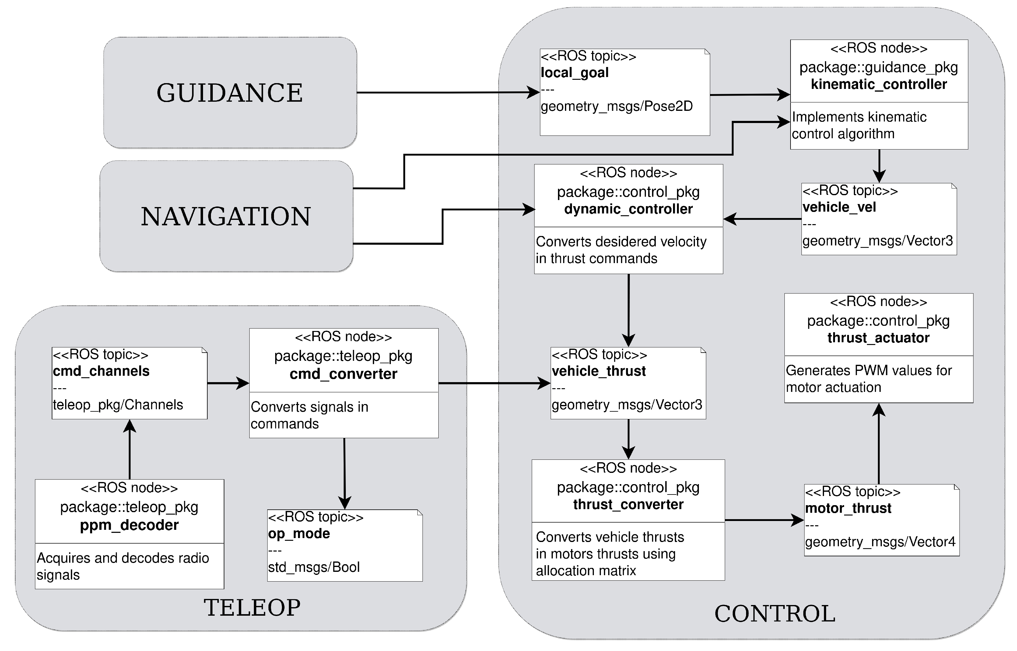
This section describes the main implemented modules that compound the base guidance, navigation and control (GNC) architecture. The design of the software architecture was focused on software modularity and components decoupling, thanks to the pub/sub paradigm and other design patterns provided by ROS. Modular software and a GNC architecture allow us to improve the components’ reliability and make it easy to enhance a single module, such as the control or planning algorithms. Figure 4 shows the main modules that compose the software architecture; for each module, a package containing the nodes needed to implement specific functionalities is created.

3.1. Robot Operating System

ROS is a framework known as a meta-operating system as it exports the main features provided by a usual operating system. Among these, ROS provides hardware abstraction, device drivers, rules and conventions, packet management systems, libraries that implement commonly used algorithms, multithreading management, interprocess communication and message passing. ROS refers to a node as the smallest unit of the processor running, and it is recommended to create one single node for each purpose, in order to improve the decoupling and reusability of the code. Nodes can exchange information with each other using different mechanisms made available by ROS:

• Topic: Through the pub/sub paradigm, one or more nodes can subscribe to a topic of interest on which, on the other hand, publishers nodes can share information. Each time a message is published on the topic, all the nodes subscribed to it receive a notification with the shared information.
• Service: It is a client/server mechanism which can be seen as a synchronous remote procedure call, i.e., it allows one node to call a function that is executed by another node.
• Action: It is a more sophisticated method of internode communication that uses topic to establish asynchronous bidirectional communication. Similar to the service mechanism, an action is taken when the server takes longer to respond after receiving a request (long-running activity), allowing a node to get intermediate responses and the ability to cancel the task at any time.

3.2. Guidance

The main purpose of the guidance module, whose details are summarized in Figure 5, is to establish the desired path of travel from the vehicle’s start position to a target location, also called goal. This task can be done using several well-known path planning heuristic or nonheuristic algorithms that can be developed using different techniques. Among these, some of the best-known techniques include artificial potential field algorithms, firstly introduced by Khatib in [25], sampling-based algorithms, such as probabilistic roadmap, or search-based algorithms, which exploit base graph theory to compute the shortest path between the source node and the target node using algorithms such as Dijkstra’s or A*. When a priori information about the environment is known, the path planning problem is solved by a module called global path planner. The information about the environment is firstly loaded with the aim to build a map, then a global path planning algorithm can be executed to find the best way to move the vehicle from the start pose to a goal pose.

The vehicle should ideally move through the planned path, but in a real scenario, the described path can be affected by several sources of error, such as unmodeled dynamics, environmental disturbances or the presence of unmapped obstacles. In this scenario, another unit, called local path planner, takes action. Its purpose is to generate local corrections to the original trajectory and allow obstacle avoidance. The guidance module contains native ROS libraries, known as navigation stack, and some custom nodes to perform its tasks. The navigation stack is made up of some packages that can be used to perform autonomous robot navigation both in a simulated and real environment. In particular, a global path planner which implements Dijkstra’s algorithm (refer to the pseudo code reported in Algorithm 1 below for details) was used among the features exported from the navigation stack as well as a set of tools to manage maps, including loading and cost map building.

Algorithm 1: Dijkstra

1: Input: s; 2: Output: $dist\left[\right]$; 3: for  $q\in N\sim \left\{s\right\}$do 4:     $dist\left[q\right]\leftarrow \infty$; 5: end for 6: $S\leftarrow \varnothing$; // visited nodes set 7: $Q\leftarrow V$; // vertices set 8: while  $Q\ne \varnothing$ do 9:     pop q from Q 10:     $S\leftarrow S\cup \left\{q\right\}$; 11:     Build neighbors set $N_s$; 12:     for $q^{\prime }\in N_s$ do 13:         if $dist\left[q^{\prime }\right]>dist\left[q\right]+distance(q,q^{\prime })$ then 14:            $dist\left[q^{\prime }\right]\leftarrow dist\left[q\right]+distance(q,q^{\prime })$ 15:         end if 16:     end for 17: end while 18: return $dist\left[\right]$

Using a modular design approach, the guidance module is a nutshell that exposes a single interface that allows communication with other modules. In particular, the manager module communicates to the guidance module the target point that should be autonomously reached. To further explain, to perform communication with the manager module, the ROS action mechanism is used, which requires the implementation of a ROS node that works as an action server. The goto_server node implemented waits for an incoming action request from the manager module, which contains the target pose expressed as $[x^{*},y^{*},{\vartheta }^{*}]$. The target is published on the topic global_planner/goal, and these messages are read by the global_planner node that computes the complete path from the start position to the target goal in terms of a set of waypoints through the map. This collection of intermediate points is processed by the local_extractor node which proceeds to send one at a time to the control module and waits for the confirmation that the single target is reached; only after having exhausted the list of waypoints is a message sent to the action server to terminate the requested action.

3.3. Navigation

The aim of the navigation module is to provide an accurate estimation of the vehicle’s position, orientation and velocities, in order to make the control and guidance modules work properly (refer to Figure 6 for details about the navigation module). For this reason, the navigation module is responsible for interfacing with the sensors, providing an abstraction layer that hides the sensor hardware and providing device drivers to interface with them. The management of the IMU is done using the imu_sensor node, which reads the IMU measurement (roll–pitch–yaw angles, linear accelerations and angular velocities) and starts to publish them on topics. For the GPS module, the ethz_piksi_ros external libraries were used to interface with the hardware device. This module provides the drivers and the libraries needed to support RTK (real-time kinematic) technologies. RTK GPS technology allows corrections to be made thanks to the use of two or more receivers: a fixed one (referred to as a base) and a mobile one (which often takes the name of rover). The base, whose position on earth is well-known, calculates an estimation of the position using the information received from the satellites and compares it with its real position, then the difference between the two is used to determine correction terms. These data are sent, usually via radio modem, to the rover’s GPS receiver, which use them to correct its error and locate itself with better accuracy. Thanks to the RTK technology, the position error decrease, providing centimeter precision.

The information coming from the IMU and GPS is combined using a sensor fusion algorithm, which merges information to obtain the vehicle state (composed of position and velocities). To this aim, in order to perform the sensor data fusion action, the extended Kalman filter (EKF) or, alternatively, the unscented Kalman filter (UKF) can be used (details about the EKF and UKF implementations are provided in the following sections). Note that the state estimations are provided by the navigation module as inputs to the control algorithms, with a sample rate of 10 Hz.

3.3.1. Extended Kalman Filter

The Kalman filter (KF) is one of the most widely used methods for tracking and estimation due to its simplicity, optimality, tractability and robustness. However, the application of the KF to nonlinear systems can be difficult. The most common approach is to use the extended Kalman filter (EKF) [26], which simply linearizes the nonlinear model along the trajectory so that the traditional linear Kalman filter can locally be applied at each computational step. Let us consider the following nonlinear discrete-time system

$$\begin{array}{ccc}\hfill {\xi }_k& =& f_{k-1}\left({\xi }_{k-1}\right)+w_{k-1},\hfill \end{array}$$

(4)

$$\begin{array}{ccc}\hfill z_k& =& h_k\left({\xi }_k\right)+{\sigma }_k\hfill \end{array}$$

(5)

where ${\xi }_k$ represents the state vector of the system, $z_k$ the measurement vector, $w_k$ the noise process due to disturbances and modeling errors and ${\sigma }_k$ the measurement noise. It is assumed that the noise vectors $w_k$ and ${\sigma }_k$ are zero-mean, uncorrelated and with covariance matrices $Q_k=Q_k^T>0$ and $R_k=R_k^T>0$, respectively, i.e., $w_k\sim \aleph (0,Q_k),{\sigma }_k\sim \aleph (0,R_k)$ The signal and measurement noises are assumed uncorrelated also with the initial state ${\xi }_0.$ Then, the estimation problem can be stated, in general terms, as follows: given the observations set $Z_k:=\{z_0,z_1,\dots ,z_k\}$, evaluate an estimate ${\widehat{\xi }}_k$ of ${\xi }_k$ such that a suitable criterion is minimized. In the sequel, we consider the mean squared error estimator, and therefore, the estimated value of the random vector is the one that minimizes the cost function

$$J\left[{\widehat{\xi }}_k\right]=E\left[{({\xi }_k-{\widehat{\xi }}_k)}^2\right|Z_k]$$

(6)

At each time instant $k,$ the EKF design can be split into two parts: time update (prediction) and measurement update (correction). In the first part, given the current estimates of the process state ${\widehat{\xi }}_{k-1}$ and covariance matrix $P_{k-1}$ and based on the linearization of the state Equation (4)

$${\mathrm{\Phi }}_k={\left.\frac{\partial f_k}{\partial \xi }\right|}_{\xi ={\widehat{\xi }}_{k-1}}$$

(7)

the updating of the covariance matrix and state prediction ${\widehat{\xi }}_{k|k-1}$ are performed as follows

$$\begin{array}{ccc}{P}_{k|k-1}& =& {\mathrm{\Phi }}_k{P}_{k-1}{\mathrm{\Phi }}_k^T+Q_{k-1},\\ {\widehat{\xi }}_{k|k-1}& =& f_k\left({\widehat{\xi }}_{k-1}\right)\end{array}$$

(8)

Then, given the current measurement $z_k$ and by linearizing the output Equation (5) according to

$$H_k={\left.\frac{\partial h_k}{\partial \xi }\right|}_{\xi ={\widehat{\xi }}_{k|k-1}}$$

(9)

the following Kalman observer gain is derived

$$K_k=P_{k|k-1}{H}_k^T{(R_k+H_k{P}_{k|k-1}{H}_k^T)}^{-1}$$

(10)

Finally, the state and the matrix covariance estimates are updated as

$$\begin{array}{ccc}\hfill {\widehat{\xi }}_k& =& {\widehat{\xi }}_{k|k-1}+K_k(z_k-h_k\left({\widehat{\xi }}_{k|k-1}\right)),\hfill \end{array}$$

(11)

$$\begin{array}{ccc}\hfill P_k& =& (I-K_k{H}_k)P_{k|k-1}\hfill \end{array}$$

(12)

and the procedure is iterated.

3.3.2. Unscented Kalman Filter

It is well known that the extended Kalman filter could give rise to poor estimation performance when the plant model (4) and (5) has a highly nonlinear structure, because it does work on a linearized model of the nonlinear state space description. Such a drawback can be avoided by using a further extension of the Kalman filter: the unscented Kalman filter (UKF) [27].

The UKF is based on a different idea: the mean and the covariance matrix are updated by resorting to a deterministic sampling technique, the unscented transform, whose aim is to select an appropriate minimal set of sample points (sigma points). Hence, all the sigma points are propagated through the state transition function $f_k\left(·\right)$ and the observation function $h_k\left(·\right),$ from which both the mean and the covariance matrix of the state estimate are finally recovered.

In particular, the sigma points are selected as follows

$$\begin{array}{cc}{\left({\Xi }_{k-1}\right)}^{\left(0\right)}=\hfill & {\widehat{\xi }}_{k-1}\hfill \\ {\left({\Xi }_{k-1}\right)}^{\left(m\right)}=\hfill & {\widehat{\xi }}_{k-1}+co{l}_m\left(\sqrt{(n+\lambda )P_{k-1}}\right),\hfill \\ \hfill & m=1,\dots ,n\hfill \\ {\left({\Xi }_{k-1}\right)}^{\left(m\right)}=\hfill & {\widehat{\xi }}_{k-1}+co{l}_{m-n}\left(\sqrt{(n+\lambda )P_{k-1}}\right),\hfill \\ \hfill & m=n+1,\dots ,2n\hfill \end{array}$$

(13)

where $n=dim\left(x_k\right)$ and $\lambda ={\alpha }^2(n+\chi )-n,$ with $\alpha$ and $\chi$ some scaling factors.

Essentially the EKF algorithm consists of two phases. In the first step the sigma point predictions of the state and of the covariance error matrix are computed by

$$\begin{array}{cc}{\widehat{\xi }}_{k|k-1}=\hfill & {\displaystyle \sum _{m=0}^{2M}{\omega }^{\left(m\right)}{\Xi }_k^{\left(m\right)}}\hfill \\ P_{k|k-1}=\hfill & {\displaystyle \sum _{m=0}^{2M}{\mathrm{\Omega }}^{\left(m\right)}\left({\Xi }_k^{\left(m\right)}-{\widehat{\xi }}_{k|k-1}\right){\left({\Xi }_k^{\left(m\right)}-{\widehat{\xi }}_{k|k-1}\right)}^T+Q_{k-1}}\hfill \end{array}$$

(14)

where ${\Xi }_k^{\left(m\right)}=f_k\left({\Xi }_{k-1}^{\left(m\right)}\right).$ Then, a correction phase is performed by using the following equations

$$\begin{array}{ccc}\hfill {\widehat{\xi }}_k& =& {\widehat{\xi }}_{k|k-1}+K_k\left(Z_k-{\widehat{z}}_k^{\left(m\right)}\right)\hfill \end{array}$$

(15)

$$\begin{array}{ccc}\hfill P_k& =& P_{k|k-1}+K_k{S}_k{K}_k^T\hfill \end{array}$$

(16)

where

$$\begin{array}{c}{\displaystyle Z_k^{\left(m\right)}=h_{k-1}({\Xi }_{k-1}^{\left(m\right)}),{\widehat{z}}_k=\sum _{m=0}^{2M}{\omega }^{\left(m\right)}{Z}_k^{\left(m\right)}}\hfill \\ {\displaystyle S_k=\sum _{m=0}^{2M}{\mathrm{\Omega }}^{\left(m\right)}(Z_k^{\left(m\right)}-{\widehat{z}}_k){(Z_k^{\left(m\right)}-{\widehat{z}}_k)}^T+R_k}\hfill \\ K_k=\sum _{m=0}^{2M}{\mathrm{\Omega }}^{\left(m\right)}({\Xi }_k^{\left(m\right)}-{\widehat{\xi }}_{k|k-1}){(Z_k^{\left(m\right)}-{\widehat{z}}_k)}^T{S}_k^{-1}\hfill \end{array}$$

with ${\omega }^{\left(m\right)}$ and ${\mathrm{\Omega }}^{\left(m\right)}$ some fixed weights selected as follows

$$\begin{array}{c}{\omega }^{\left(0\right)}=\frac{\lambda }{(n+\lambda )},{\omega }^{\left(m\right)}=\frac{1}{2(L+\lambda )},m=1,\dots ,2n,\hfill \\ {\mathrm{\Omega }}^{\left(0\right)}=\frac{\lambda }{(n+\lambda )}+(1-{\alpha }^2+\beta ),\hfill \\ {\mathrm{\Omega }}^{\left(m\right)}=\frac{1}{2(n+\lambda )},m=1,\dots ,2n,\hfill \end{array}$$

where $\beta$ is a parameter used to incorporate any prior knowledge about the distribution of the state ${\xi }_k.$

3.4. Control

The main task of the control module (Figure 7) is to calculate the control law needed to reach the target pose and generate the control signal to actuate the four thrusters. The control module is mainly divided into two submodules: a kinematic controller with the aim of generating speed references to drive the vehicle to the goal, and a dynamic controller, whose task is to generate the control commands to travel at the desired speed.

3.4.1. Kinematic Controller

First, the position is defined, and the heading errors vector is the difference between the desired pose and the current pose in the horizontal plane.

$$\mathbf{e}={\eta }^{*}-\eta =\left[\begin{array}{c}{x}^{*}-x\\ y^{*}-y\\ {\vartheta }^{*}-\vartheta \end{array}\right]$$

(17)

Assuming that the reference positions are constant values, the kinematic positioning error model can be obtained by the differentiation of (17) and using (2):

$$\dot{\mathbf{e}}=-\dot{\eta }=-\mathbf{R}\left(\vartheta \right)\nu$$

(18)

Then, it is possible to design a control law in the form

$${\nu }^{*}=-\mathbf{R}\left(\vartheta \right)\left({\mathbf{K}}_{\mathbf{p},\mathbf{K}}\mathbf{e}+{\mathbf{K}}_{\mathbf{i},\mathbf{K}}\int \mathbf{e}dt\right)$$

(19)

where the controller outputs ${\nu }^{*}$ are the desired speed to be passed as input to the internal speed controller. The proportional gains ${\mathbf{K}}_{\mathbf{p},\mathbf{K}}$ and ${\mathbf{K}}_{\mathbf{i},\mathbf{K}}$ are diagonal matrices, where the ${\mathbf{K}}_{\mathbf{p},\mathbf{K}}$ components are used to improve the reactivity of the vehicle to reach the target pose and the ${\mathbf{K}}_{\mathbf{i},\mathbf{K}}$ components are introduced to compensate any constant environmental disturbances such as wind or currents. The values of the gains were empirically determined following field tests.

3.4.2. Dynamic Controller

Starting from the model in (3), thanks to the simplifications previously introduced, it is possible to design a decoupled control law, one for each direction and one for the heading speed control. The PI control law can be written as

$${\tau }_{uvr}^{*}={\mathbf{K}}_{\mathbf{p},\mathbf{D}}({\nu }^{*}-\tilde{\nu })+{\mathbf{K}}_{\mathbf{i},\mathbf{D}}\int ({\nu }^{*}-\tilde{\nu })dt$$

(20)

where ${\nu }^{*}$ is the vector of desired velocities previously computed by the kinematic controller, and $\tilde{\nu }$ is the estimated velocities vector provided by the navigation module. Moreover, for the dynamic controller, the gain matrices ${\mathbf{K}}_{\mathbf{p},\mathbf{D}}$ and ${\mathbf{K}}_{\mathbf{i},\mathbf{D}}$ are in a diagonal form, and their values are experimentally computed.

3.4.3. Thruster Controller

The thrust-commands-computed ${\tau }_{uvr}^{*}$ are transformed in the thrusters’ commands ${\tau }_{1234}$ using the pseudoinverse of the $\mathrm{\Sigma }$ matrix

$${\tau }_{1234}^{*}={\left({\mathrm{\Sigma }}^{\mathtt{T}}\mathrm{\Sigma }\right)}^{-1}{\mathrm{\Sigma }}^{\mathtt{T}}{\tau }_{uvr}^{*}$$

(21)

Then, these values are converted into the required PWM signals needed to properly actuate the motors, according to the thruster characteristic curve. The thruster characteristic was obtained using two third-degree polynomials to fit the thrust/PWM relationship obtained from the thruster datasheet.

 Remark 2. 

Note that the kinematic (19) and dynamic (20) controller must be discretized in order to provide their implementations in the ROS nodes.

4. Manager Module

Autonomous vehicles are increasingly used to perform more complex tasks during their service cycle; indeed, they are equipped with advanced sensors and payloads. This implies that moving along a path or reaching a desired pose are only the basic functions that an autonomous vehicle must have. A vehicle can be considered completely autonomous only if its payload management is also autonomous, as this allows the vehicle to operate for extended periods of time without any external interaction. In this respect, it is possible to refer to Figure 8 where the designed manager modules is outlined.

4.1. Mission Definition

A mission is any operation performed by the vehicle, which can be described as a set of elementary tasks that could be executed sequentially or concurrently. The purpose of a mission-oriented paradigm is to find a common syntax structure to model every vehicle’s behavior. This generalization requires a preliminary effort that allows the creation of an adequate structure for modeling as many behaviors as possible; this involves an increase of the degree of abstraction of the manager module, which is in charge of executing all the single tasks that compose the mission, despite its overall complexity. Therefore, it is necessary to identify a set of elementary actions provided by the vehicle, such as reaching a single point (goto task), turning on/off an onboard instrument such as a camera or sonar (inst1_pow_ON), activating an auxiliary actuator such as a winch (winch_goto), etc. Through the definition of the elementary task, it is possible to model more complex behaviors as an appropriate combination of these. For example, a patrolling mission can be modeled as a sequence of goto actions through a set of waypoints; in the same way, it is possible to describe a data collection mission as a cyclical combination of a goto task with the water immersion of the appropriate probes (i.e., using the winch), the data collection and the recovery of the probes.

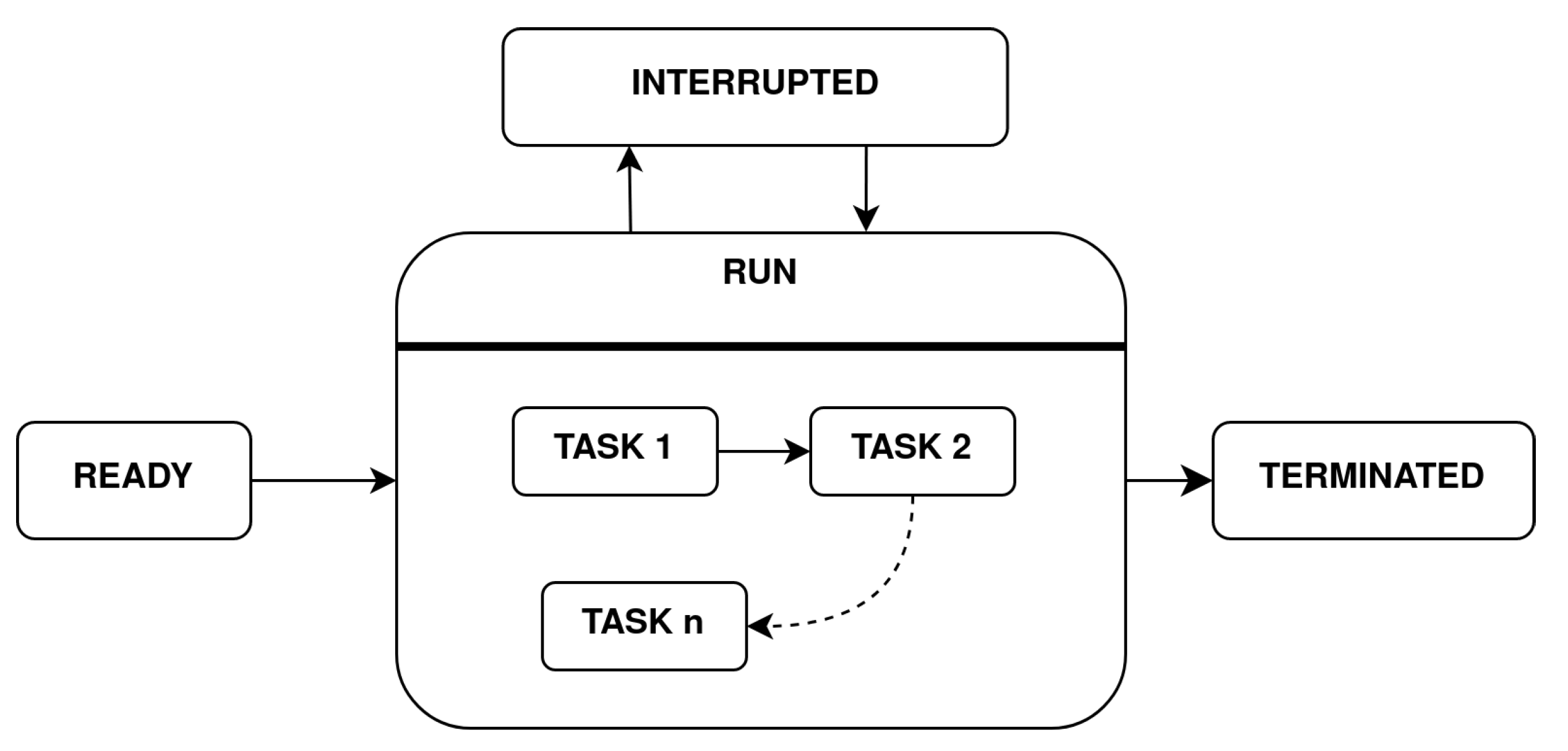
An intuitive tool suitable for modeling missions as a sequence of tasks is given by finite state machines. Each task defines a state and implements a ROS action server to perform the required job and the outcome of the action (succeeded, aborted, etc.) determines the next state to execute. The hierarchical state machine reported in Figure 9 can be used to allow missions to be interrupted by implementing a priority-based switching mechanism. Like a process in a conventional operating system, a mission can remain in one of several states:

• Ready: The mission is ready to be executed and it can join the active mission list, which contains a suitable mission to be executed. A mission in a ready state waits a start command to jump in the run state.
• Run: The mission is running (mission with the highest priority). This state contains a nested state machine that specifies the tasks to reach the mission goal. The tasks of the inner state machine are executed by sending a goal request to the appropriate ROS action server.
• Interrupted: If a higher priority mission is present, the current mission is interrupted and a mission switching is performed. The interrupted mission can restart from the beginning or from the last task executed, according to the mission policy settings.
• Terminated: when a mission is finished (the last task is completed) the mission moves in this state.

The RUN state contains nested state machines that represent the main tasks that compose a mission. These tasks can be organized in a sequential way, or they can be executed concurrently if there is no conflict in the use of the actuators. Figure 10 shows an example of how a mission containing concurrent tasks is modeled.

The implementation of a mission is done by a Mission class that contains a state machine implemented in the Automa class using the Python library SMACH [28]. The main advantages of using SMACH are the simple python-based syntax that allows to easily model hierarchical state machines, the task preemption support (used to interrupt a mission), the easy way to pass any relevant data between states, and its full compatibility with ROS. The Mission class also contains some useful parameters used to determine the mission priority or the possibility to repeat a mission more than one time (i.e., in a patrolling mission through a set of waypoints).

4.2. Mission Management

The use of the vehicle for a long period supposes the possibility of carrying out several alternating missions; this can be defined as a multimission paradigm. These missions can be time-fixed scheduled or dynamically scheduled using a priority-based mechanism. Then, the manager module selects in real time which mission has to be performed with respect to their priority, by switching between the active ones.

The mission_manager node is in charge of the decision-making mechanism used to perform dynamic mission scheduling. This node periodically computes the priority level of each ready mission and sorts them in a heap data structure. Priority computation can be done according to different policies:

• Fixed-priority scheduling: each mission has a fixed priority level that remains unchanged over time, according to the mission type.
• Dynamic scheduling: the priority level of the mission can be modified to avoid starvation (i.e., using aging mechanism) or to react to environment changes or external events.
• Smart scheduling: more powerful and sophisticated algorithms can be used to perform more efficient mission scheduling by developing AI-based algorithms.

For example, an energy consumption estimation can be done for each mission, which could be compared with the current battery level to establish the feasibility of the mission. In a long life cycle, another challenge is to provide robots with basic autonomous energy management capabilities. The vehicle should estimate in real time its residual battery level and compare it with the estimated energy needed to reach a home position to recharge its battery; if the battery level is under a safe threshold, the vehicle can increase the priority of a recharging mission with the aim to interrupt the current mission and go back to the home position. Another aspect that can be taken into account is the weather conditions, to avoid executing missions that require operation in a highly hazardous area.

The core of the scheduling algorithm is implemented in the sorting method of the mission_manager node. In addition, an external command interface is provided, which allows the user to interact with the manager module. This interface exports a set of methods suitable for adding/removing missions from the active mission list or for starting/interrupting the desired mission. Figure 11 illustrates the activity diagram of the mission_manager node, whereas the Algorithm 2 below shows in pseudocode the core implementation of the scheduler’s life cycle.

Algorithm 2: Mission Management

1: heap = [ ] 2: heap $\stackrel{}{\leftarrow }$ load missions 3: cur_mission = None 4: heap $\stackrel{}{\leftarrow }$ sort missions 5: if current_mission ≠ heap[0] then 6:     if current_mission ≠ None then 7:         stop current_mission 8:     end if 9:     current_mission = heap[0] 10:     start current_mission 11: end if 12: if current_mission is terminated then 13:     remove heap[0] 14:     current_mission = heap[0] 15:     start current_mission 16: end if 17: goto 4

5. Experimental Results

Several experiments were accomplished in a real environment to test the different components of the prototype vehicle and its capability to perform a task. In view of this, Section 5.1 reports the tests conducted to validate the presented multimission approach. Firstly, in order to validate the proposed common state machine structure, the execution of a simple single mission was performed. Then, the proposed multimission priority-based switching mechanism was tested by considering a more complex scenario involving two simultaneous missions. Moreover, the tests focused on the validation in a real environment of the whole GNC architecture and hardware design presented in Section 5.2.

5.1. Single- and Multimission Management Test

This section is devoted to verifying the effectiveness of the mission management module by accounting for both the execution of a simple mission and concurrent missions. Then, a scenario involving two simultaneous missions is validated.

In the first test, a single patrolling mission (missione1) was loaded in the manager module and the correctness of the state machine execution was verified. In addition, concurrent tasks were tested to prove that the movement tasks were executed while other tasks, that used, for example, any payload, executed other operations. The left side of Figure 12 shows the debug flow of the hierarchical state machine operations. Underlined in yellow are the executed elementary states, and underlined in orange are the state outputs that lead to a state transition. The red section shows that the transition from the RUN state to the TERMINATED state happens when both the concurrent state machines finish their tasks.

The right side of Figure 12 shows the execution flow of a multimission scenario: while the mission missione1 was executing, another more priority mission was loaded and the mission_manager scheduling algorithm switched the two missions as soon as possible. In the figure, the manager module operations that start/stop the missions are highlighted.

5.2. Real Environment Test

Other kinds of tests were carried out in order to evaluate the behavior of the whole architecture, first using the simulation environment provided by ROS. To this purpose, Rviz and Gazebo were used, and a kinematic model of the vehicle was built in order to validate the movement tasks. Then, different tests in a real environment were conducted, both on sea and lake surfaces. The goal was to show the capabilities of the vehicle to move in autonomous mode among several waypoints. Moreover, a performance evaluation in terms of tracking error was performed.

5.2.1. Test 1

The first experiment was conducted in a sea environment, starting from a beach located in the little town of Falconara Albanese (CS) in Calabria: the vehicle was powered on next to the fixed base (red marker in Figure 13) positioned on the beach and then, it was remotely guided next the first waypoint. When the mission was enabled, it started to move in autonomous mode among four waypoints (blue markers in Figure 13) provided by global coordinates. At the end of the mission, the vehicle was guided towards the beach. The calm environment conditions allowed us to register a maximum positioning error of less than $0.5$ meters, where the position error $e\left(t\right)$ was defined as the difference between the straight line that connects two waypoints and the real trajectory that the vehicle traveled to reach the next waypoint. In this respect, Figure 14 reports the results of data elaboration activity while Figure 15) shows the absolute value of tracking error $e\left(t\right)$. We highlight that for applications such as environmental monitoring and divers support, errors less than two meters are acceptable.

5.2.2. Test 2

The second test was accomplished in a lake environment, next to the town of Petronà (CZ) in Calabria. In this scenario, the vehicle moved among the side of a triangle expressed with respect to the local reference system (Figure 16). Analyzing the data collected (shown in Figure 17) from the vehicle, the maximum tracking position error recorded was less than 0.7 m. Notice that the maximum error (refer to Figure 18) in the lake test was greater than that in the sea test due to windy conditions on that test day.

6. Conclusions

In this paper, the basic steps toward an ASV prototype development were presented, with the main focus on the GNC software architecture implementation and its extension with a management module, to accomplish high-level mission scheduling in a dynamic environment. All software and hardware modules of the designed prototype were validated in a real environment and the performed tests showed that the vehicle was capable of good performance. Moreover, it is important to highlight that the introduced manager module is ready to implement more sophisticated AI-based algorithm to better accomplish a decision-making process on mission scheduling in a dynamic environment where mission priority can change due to safety reasons or real-time event occurrence. Future works could define accurate mission priority assignment criteria, in order to provide dynamic mission switching according to the scheduling algorithm discussed in Section 4. The proposed architecture is currently undergoing improvement in order to support multivehicle cooperation and a high-level reference supervision scheme by adding appropriate modules in the guidance package [29].