Article

UAS Hyperspatial LiDAR Data Performance in Delineation and Classification across a Gradient of Wetland Types

1
Department of Earth and Ocean Sciences, University of North Carolina Wilmington, 601 S. College Rd., Wilmington, NC 28403, USA
2
Department of Mathematics and Statistics, University of North Carolina Wilmington, 601 S. College Rd., Wilmington, NC 28403, USA
*
Author to whom correspondence should be addressed.
Drones 2022, 6(10), 268; https://doi.org/10.3390/drones6100268
Submission received: 19 August 2022 / Revised: 15 September 2022 / Accepted: 19 September 2022 / Published: 22 September 2022
(This article belongs to the Special Issue Drones for Rural Areas Management)

Abstract

:
Wetlands play a critical role in maintaining stable and productive ecosystems, and they continue to be at heightened risk from anthropogenic and natural degradation, especially along the rapidly developing Atlantic Coastal Plain of North America. As such, strategies to develop up-to-date and high-resolution wetland inventories and classifications remain highly relevant in the context of accelerating sea-level rise and coastal changes. Historically, satellite and airborne remote sensing data along with traditional field-based methods have been used for wetland delineation, yet, more recently, the advent of Uncrewed Aerial Systems (UAS) platforms and sensors is opening new avenues of performing rapid and accurate wetland classifications. To test the relative advantages and limitations of UAS technologies for wetland mapping and classification, we developed wetland classification models using UAS-collected multispectral and UAS-collected light detection and ranging (LiDAR) data relative to airborne-derived LiDAR models of wetland types ranging from palustrine to estuarine. The models were parameterized through a pixel-based random forest algorithm to evaluate model performance systematically and establish variable importance for a suite of variables including topographic, hydrologic, and vegetation-based indices. Based on our experimental results, the average overall classification accuracy and kappa coefficients for the UAS LiDAR-derived models are 75.29% and 0.74, respectively, compared to 79.80% and 0.75 for the airborne LiDAR-derived models, with significant differences in the spatial representation of final wetland classes. The resulting classification maps for the UAS models capture more precise wetland delineations than those of airborne models when trained with ground reference data collected at the same time as the UAS flights. The similar accuracy between the airborne and UAS models suggest that the UAS LiDAR is comparable to the airborne LiDAR. However, given poor revisit time of the airborne surveys and the high spatial resolution and precision of the UAS data, UAS-collected LiDAR provides excellent complementary data to statewide airborne missions or for specific applications that require hyperspatial data. For more structurally complex wetland types (such as the palustrine scrub shrub), UAS hyperspatial LiDAR data performs better and is much more advantageous to use in delineation and classification models. The results of this study contribute towards enhancing wetland delineation and classification models using data collected from multiple UAS platforms.

1. Introduction

Coastal plain wetlands are low-gradient, low-lying areas of land characterized by hydrophilic vegetation, hydric soils, and remarkable levels of biodiversity that play important roles in maintaining productive ecosystems [1,2,3]. Wetland ecosystems are home to diverse wildlife and vegetation species and provide many societal benefits such as improved water quality, flood and carbon storage, erosion shoreline and infrastructure protection, and support for tourism, hunting, and fishing as local livelihood sources [4]. However, wetland extent and condition have been under increasing pressure from anthropogenic and natural drivers in the last half-century [5,6]. Urbanization, agricultural development, and silviculture continue to be major human drivers of wetland loss today, in addition to climate change stressors. Sea-level rise and increases in hurricane and storm intensity and frequency pose serious risks to fragile coastal wetland ecosystems, through inundation, saltwater intrusion, and the slow alteration of wetland types and composition, in particular [7]. Combined, these factors resulted in significant wetland losses at an average rate of about 80,000 acres per year between 2004 and 2009 in the United States alone [8]. The consequences of wetland loss, both in terms of extent and functionality, manifest themselves directly and indirectly on surrounding ecosystems and the organisms that rely on wetlands. Given that 43% of the USA’s endangered and threatened species rely on wetlands for their survival, wetland loss compounds ecosystem degradation and has important tropic chain repercussions [9].
Wetland delineations and classifications have been conducted numerous times since as early as the 1700s as a means to inventory wetlands for many purposes, including natural resource research and conservation management [10]. Wetland maps are used for environmental impact and water quality assessments, hydrological and climatological modeling, transportation planning, identification of conservation or ecological restoration opportunities, and outreach and education to the general public [11]. Therefore, developing a record of wetland extent, location, and type, especially in the context of coastal wetland habitats, provides critical information for policy and decision making and contributes to protecting fragile wetland ecological systems and overall coastal resilience.
Due to their importance and significant coastal wetland losses in the last half-century, increasing attention has been paid to developing up-to-date and higher-accuracy wetland classifications. However, wetland identification and delineations in the primarily forested Coastal Plain region of the USA are labor-intensive, time-consuming, and costly. Most coastal wetlands are dominated by thick forest cover and/or muddy ground unlike grass or non-forested wetlands, making even locations that are not very remote difficult to access and prone to physical degradation during fieldwork [12,13]. For example, in the state of North Carolina (NC) alone, primarily forested coastal plain wetlands cover approximately 76.3% (3,100,703 acres) of total wetland areas [11], yet the most recent wetland cover dataset for this area was completed as part of the National Wetlands Inventory (NWI) between 2001–2010 (Figure 1). The estimated cost of field-based wetland delineation in eastern NC ranges from $120–180 per acre and can take several weeks to complete for a relatively small site (2000–3000-acres) (NC Department of Transportation (NC DoT) personal communication, 1 September 2021). The extensive spatial scale of wetlands in NC translates into increased cost and manpower required to conduct ground surveys, which makes it very difficult to maintain regularly updated wetland maps, especially for purposes of planning for new or updated transportation and construction projects. As such, wetland delineations and classifications based on remotely sensed data are common in filling the gaps between field delineations. We aimed to provide an assessment of the feasibility of using UAS surveys to fill this gap and provide avenues for rapid wetland assessments with lower reliance on field campaigns.
Remote sensing technologies have often been used as a tool to tackle issues associated with traditional wetland surveys [12,14,15,16,17]. Remote sensing imagery, whether from satellite, airborne sources, or, more recently, UAS, enables wetland researchers to access data for areas that are physically inaccessible to surveyors and takes significantly less time than an on-foot survey to collect Earth surface data with minimal disturbance to the surveyed areas [18,19,20]. Studies show the effectiveness of combining multispectral and LiDAR datasets for wetland classification [21,22]. While multispectral data can provide spectral reflectance information to classify vegetation, soil, and manmade objects in an image, LiDAR data can offer proxies for hydromorphology by measuring and detecting subtle changes in elevation or vertical vegetation structural information. Hyperspatial UAS data in particular can result in products with much enhanced spatial resolution and detail given the much higher point densities resulting from surveys at lower flight altitudes using multiple laser beams [12,13]. Secondly, UAS LiDAR is timely, can be flown much more rapidly than airborne missions, which take years to plan, and therefore the UAS LiDAR can be planned and deployed very quickly and respond to natural and anthropogenic events (floods, storm impact assessments, urban developments, etc.). Thirdly, hyperspatial UAS LiDAR can provide modeling inputs that can further utilize high resolution canopy height and closure metrics to refine vegetation classification models. Research shows that the accuracy of land cover classifications improves when combining multispectral and LiDAR data, in addition to any filed collected data [21,23]. However, to the authors’ knowledge, the fusion of hyperspatial LiDAR and multispectral data collected via UAS platforms for wetland classification remains largely unexplored. Hyperspatial resolution from UAS LiDAR is relatively new and enables more precise landscape features to be quantified, especially when dense vegetation in present. Given the low-lying and minimal topography variations of coastal wetlands, typical workflows and datasets to obtain hydrologic indices and drainage patterns tend to not work as effectively as they would in areas of more defined terrain [23,24]. However, despite the usefulness of hyperspatial data in detecting small-scale landscape features, data volumes can hamper the effectiveness of traditional remote sensing classification techniques. Machine learning (ML) algorithms are becoming commonplace as data volumes and dimensionality increase and specifically, random forest models have proved useful in predicting costal wetland areas given their ability to handle both continuous and categorical data and high dimensionality of data with strong correlations among features [25,26].
To determine the performance of UAS-collected LiDAR data relative to airborne, large-area LiDAR collections, we tested wetland delineation and classification models for coastal plain areas using UAS-collected multispectral and LiDAR derivatives through pixel-based random forest algorithms (UAS hyperspatial LiDAR + UAS multispectral vs. aircraft non-hyperspatial LiDAR + UAS multispectral model combinations). We addressed the following specific research questions:
(1) How accurate are UAS-collected multispectral and hyperspatial LiDAR datasets in predicting wetland presence (delineation) and type (classification) when compared to airborne non-hyperspatial LiDAR data?
(2) What are the most important variables that predict wetland presence and type along a range of estuarine to palustrine wetland types on the Atlantic Coastal Plain?
The main objectives of this study, therefore, were to build and demonstrate a methodology that uses UAS-collected passive and active remote sensing data along with airborne active remote sensing LiDAR data for wetland classification. To answer the research questions, two specific research objectives were defined:
(1) Quantify and visualize the results of random forest models that predict wetland types with LiDAR-derived topographic indices [23] and multispectral data and determine the best fit model relative to field-collected wetland data.
(2) Determine the most important topographic and vegetation condition variables that can be used for predicting wetland presence and types across a gradient of wetland composition and types.

2. Materials and Methods
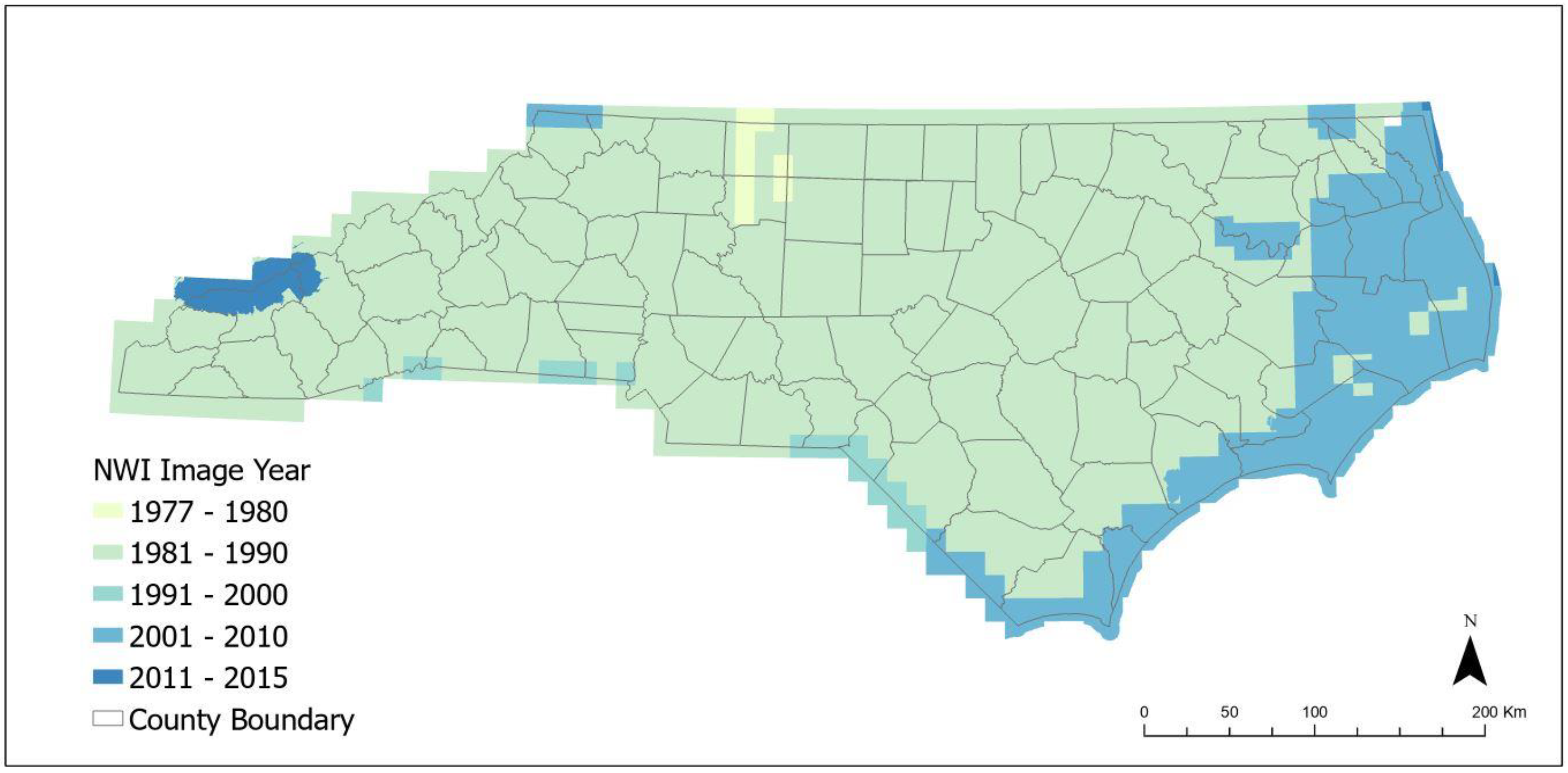
2.1. Study Sites

This study was undertaken in four Coastal Plain sites of southeastern North Carolina, USA (Figure 2), to include various wetland types and topography. They are in the warm oceanic climate/humid subtropical climate, based on the Köppen climate classification. This region has hot summers, warm falls and springs, and cool winters. The summer temperatures range from 26 °C to 37 °C (78 °F to 98 °F) in the hottest months, and the winter months bring the temperature down to about 4 °C (39 °F). The study sites include four wetland types based on the Cowardin system: estuarine intertidal emergent (E2EM), palustrine forest (PFO), palustrine emergent (PEM), and palustrine scrub-shrub (PSS) (Figure 2, Table 1) [27]. In this paper, we describe the wetland classes as the class codes as shown in Table 1. Non-wetland areas are classified as water or non-wetland area.
Site 1 (Maysville, Jones County, 77°14′17″ W, 34°54′1″ N) is mainly a palustrine forested wetland with open upland grasslands, and the site sits more inland than any other site, meaning this area is less influenced by tidal effects and hydrologically connected to the estuary of the New River, but there is a small stream running through the study area that is covered by a relatively dense canopy. Site 2 (Surf City, Pender County, 77°33′15″ W, 34°26′24″ N) is located next to Topsail Sound, where there is a strong tidal influence on the northeast side of the area. The site has a mix of estuarine with low-water resistant grass and a pine tree-dominated riverine wetland system (Pinus taeda and Pinus palustris). Site 3 (Masonboro Island, New Hanover County, 77°49′39″ W, 34°10′15″ N) is on the island located between the barrier island towns of Wrightsville Beach and Carolina Beach. The variety of its topography includes subtidal soft bottoms, tidal flats, hard surfaces, salt marshes, shrub thicket, maritime forest, dredge spoil areas, grasslands, ocean beaches, and dunes. This island is the largest undisturbed barrier island along the southern part of North Carolina [28]. Lastly, site 4 (River Road, New Hanover County, 77°55′11″ W, 34°5′12″ N) runs parallel to the Cape Fear River, creating a tidally influenced environment with low salinity called a palustrine wetland system, with riverine wetlands inland from the estuary. The palustrine area is characterized by low-growing and water-resistant vegetation while the riverine areas are dominated by thick pine tree forests. The National Wetland Inventory (NWI) dataset was used to initially show wetland class distributions (Figure 1) and to calculate the distributions of wetland classes of each site summarized in Table 2.

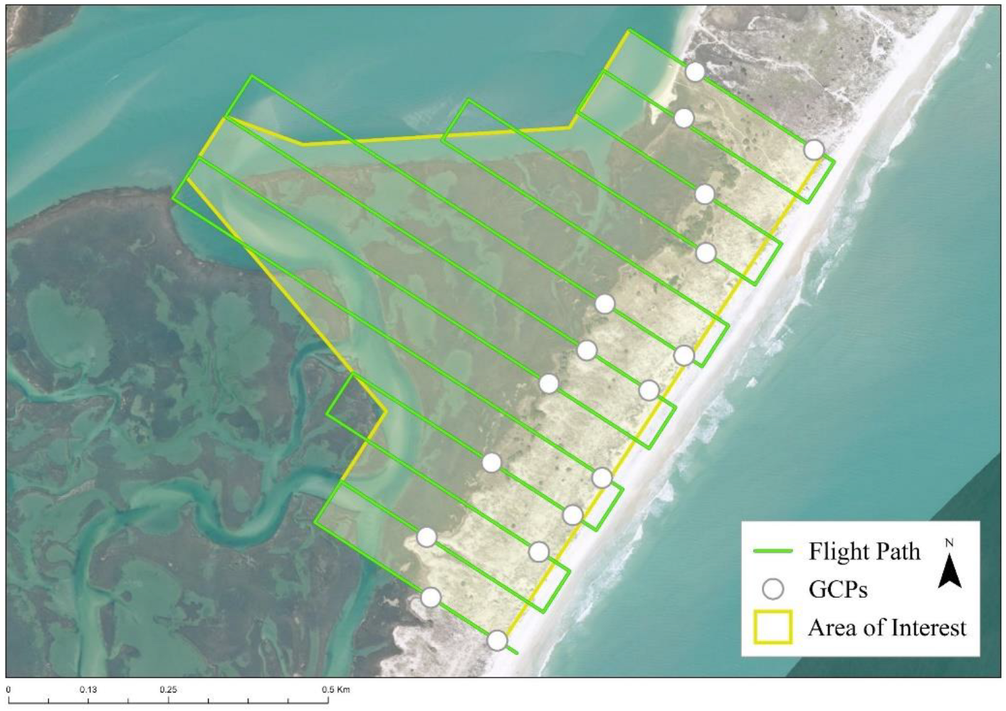
2.2. Data Acquisition

Fieldwork was conducted between October of 2020 and January of 2021 (Table 3) and consisted of same-day UAS multispectral and LiDAR missions supplemented by in situ ground reference data used to train and validate classification models. Additionally, statewide airborne LiDAR data were also used to compare the effectiveness of the UAS LiDAR data for wetland classification. The four respective datasets are described in detail in the following four sections.

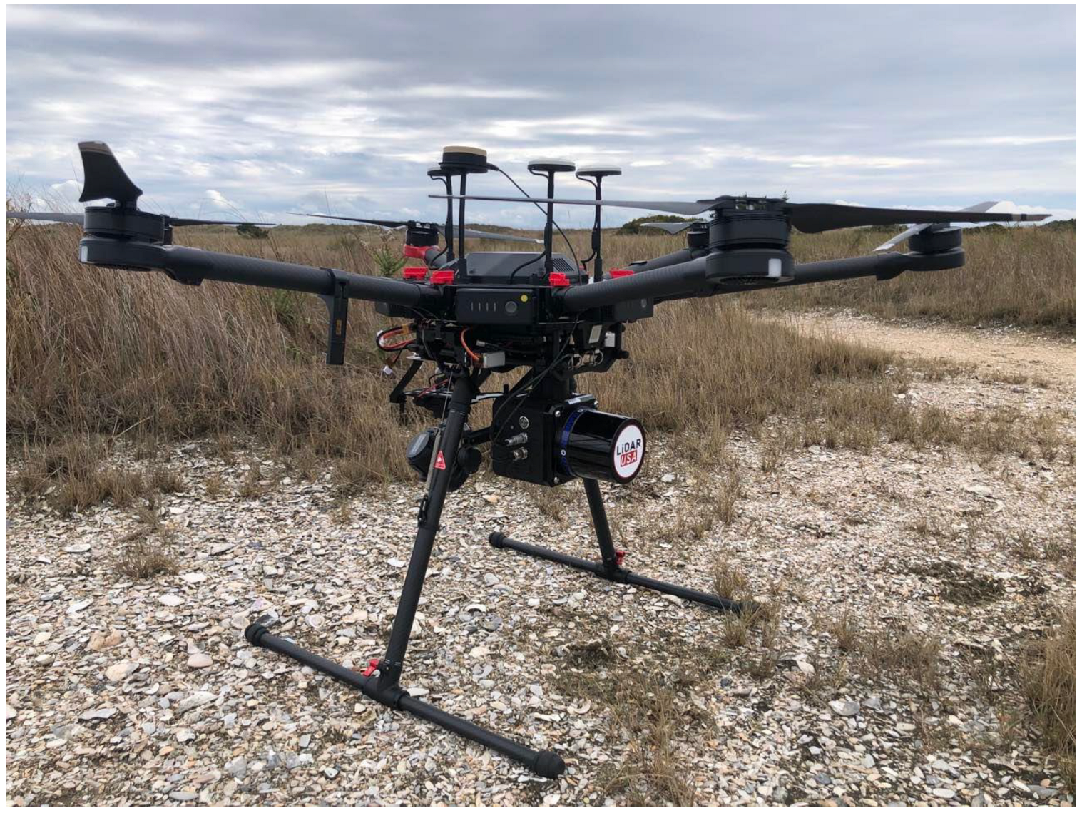
2.2.1. UAS LiDAR Data

The Quanergy M8 LiDAR (manufactured by LiDAR USA) sensor carried by the DJI Matrice Pro (M-600 Pro, manufactured by DJI, Beijing, China) was used to collect hyperspatial LiDAR data (Figure 3). The Quanergy M8 Core is an eight-laser scanner with a slightly larger range at 150 m (accuracy of 5 cm) (Table 4). It has a 360-degree horizontal FOV and 20 vertical FOV and weighs 800 g. The Quanergy M8 is reported to collect up to 420,000 points per second using time-of-flight (TOF) depth perception, and the point density is between 350 and 400 points/m2 with the altitude and spacing settings. The M600 Pro is a six-armed rotocopter with an onboard A3 Pro flight controller system comprising three inertial measurement units (IMUs) and three global navigation satellite system (GNSS) units. IMUs and GNSS units work together to maintain a reliable and precise flight path and to reduce the risk of system failure. This LiDAR system was acquired by PI Pricope under the NC Department of Transportation Environmental Analysis Unit contract RP-2020-04 in March 2020.
Flight missions were designed in ArcGIS Pro (Figure 4) and implemented using an automated flight planning application called DJI Ground Station Pro (https://www.dji.com/ground-station-pro) with a flight altitude of 55 m (180 ft), flight transect spacing of 76 m (250 ft), and flight speed of 12 m/s for all sites. Those parameters were set to ensure adequate overlap between the flight lines given the range and horizontal and angular field of view of the LiDAR scanner. The accuracy of the flight path is ensured by two systems complementing each other: the inertial navigation system (INS) and GNSS built into the Quanergy sensor and Matrice M8 drone, respectively. The INS, which is built into the LiDAR sensor, computes a relative position from an initial starting point, while the Matrice aircraft collects GNSS data from orbiting satellites to calculate the absolute position, time, and velocity.
To ensure reliable and high-accuracy end products, each UAS LiDAR field survey conducted also included the collection of GNSS data using on-the-ground Trimble units. Ground control points (GCPs) were surveyed with the Observed control point method to improve and test end-product accuracy using a Trimble R10 GNSS RTK system. An average of twelve GCP targets was placed under each flight path for maximum point density on the target surface [29,30]. The initial GCP coordinates were obtained by orbital satellite information, and these coordinates had subsequent differential corrections at centimeter-level accuracy using the North Carolina GNSS Real-Time Network (RTN). The RTN received GNSS data from the North Carolina Continuously Operating Reference Station (CORS) network of base stations to correct errors for each second of time. The correction data were sent to the Trimble rover in the field via the Internet allowing us to obtain centimeter-level positional accuracies of GCPs horizontally and vertically. In addition to the GCP survey, a rapid static survey was conducted with a Trimble R8 GNSS real-time kinematics (RTK) system to collect elevation data to test the accuracy of the end product.

2.2.2. UAS Multispectral Data

Multispectral imagery (green, red, red-edge, and near-infrared) was collected using a Parrot Sequoia+ sensor (1.2 megapixels for the multispectral bands) on the same date as the UAS LiDAR survey. The sensor was carried by a SenseFly eBee Plus fixed-wing UAS with an on-board RTK receiver (Table 5). We used the eMotion flight planning software for all phases of flight planning and implementation. The same areas of interest for each LiDAR collection were used for the multispectral data collections.
Multispectral imagery was collected at a 60% lateral and 80% longitudinal overlap. The ground sampling distance (GSD), based on a flight altitude of 119 m (400 ft) above mean sea level for all flights, was approximately 13.0 cm/pixel for the final reflectance data. All reflectance data were calibrated in the field before each flight using a Parrot calibration target. Additionally, the same GCPs were used for both LiDAR and multispectral surveys.

2.2.3. Field Sampling

Wetland habitat data were collected in the field as ground reference data. The data were used for training models and testing the model accuracies. Habitat reference data consisted of point data with wetland classes and their locational information. To minimize the human bias in selecting the locations of reference data, random sample locations were generated before the fieldwork. The NWI dataset was used as reference data to map the distribution of wetland classes in each study site. Locations of habitat points were generated using the Create Random Points tool in ArcGIS Pro. Our goal was to have 15 reference points for each wetland class and 50 points for the non-wetland areas to ensure appropriate class representation. Because non-wetland areas were generally more accessible and included multiple types of land cover such as upland grass, artificial surfaces, and open water, more habitat points were collected in these classes than wetland classes.
Habitat points were collected in the field (on the same day as the UAS surveys) using a Trimble R10 GNSS RTK System using the Topo points method. Habitat points were collected as close to the randomly generated points as possible, and each point was recorded with a wetland class that was ground-verified. However, many of the planned points were physically impossible to access because of topography, vegetation cover, or inundation level during data collection. Therefore, the rest of the habitat points were created using visual inspections of wetland classes using 2020 National Agriculture Imagery Program (NAIP) imagery. The NAIP imagery is open-source data and can be downloaded from the Geospatial Data Gateway of the United States Department of Agriculture (USDA) at https://datagateway.nrcs.usda.gov/GDGHome_DirectDownLoad.aspx. The 2020 true color NAIP imagery was the best option for this project because the LiDAR and habitat points were collected in the same year or one year later (2020 and 2021). The remaining planned habitat points were overlaid with the true color 2020 NAIP imagery in ArcGIS Pro, and wetland classes were defined for the original planned sampling points, including a confidence level.

2.2.4. Airborne LiDAR Data

The second LiDAR dataset used for this research to compare the performance of hyperspatial LiDAR data (UAS Quanergy LiDAR) was the North Carolina Quality Level 2 (QL2) LiDAR data. The main difference between the two LiDAR datasets, aside from the method of collection, is the point density. While the point density of Quanergy LiDAR is 350 to 400 points/m2, that of QL2 LiDAR is only 2 points/m2 on average. The North Carolina Risk Management Office provides the QL2 data that are publicly available from the Spatial Data Download portal at https://sdd.nc.gov/. The QL2 LiDAR data was collected between January 30 and March 13 of 2014. Three airborne sensors were used for the airborne LiDAR surveys: two Leica ALS70HP and an Optech Pegasus HA500 (Table 4). All data were collected during leaf-off conditions, and coastal areas were surveyed during the low tide conditions. The reported accuracy for QL2 data in the study area has a root-mean-square error of z (RMSEz) for vegetated and non-vegetated areas at 9.0 cm and 6.9 cm, respectively. Even though the QL2 is six to seven years older than the 2020 and 2021 Quanergy LiDAR data, it was the only LiDAR dataset available to use as a reference as of December 2021.

2.3. Data Processing

The data processing and analysis consisted of three phases: (1) data preprocessing, (2) derivation of topogeomorphic and vegetation indices, and (3) model configuration and coding (Figure 5), detailed sequentially below. It should be noted that the NAD 1983 State Plane North Carolina FIPS 3200 (meters) projected coordinate system and NAV88 Geoid 12A were used for all datasets and map products throughout this research.

2.3.1. Preprocessing

Initial preprocessing involved using raw LiDAR and multispectral data in conjunction with other field-collected data (such as static data and/or GCPs) to georeference and project the point clouds. Preprocessing Quanergy LiDAR data consisted of three phases: (1) resolving kinematic corrections for aircraft position data using aircraft GPS and static ground data, (2) calculating the laser point position, and (3) removing noise and assessing vertical accuracy. First, the LiDAR datasets were referenced to static and aircraft GNSS data, collected by the Trimble system and a GPS receiver in the Matrice 600, respectively, during the LiDAR collection. The static data were downloaded from the Trimble receiver, transformed into a Receiver Independent Exchange Format (RINEX) file, and processed using Online Positioning User Service (OPUS) solution at https://geodesy.noaa.gov/OPUS/ to increase the precision of the base station data. Inertial Explorer (NovAtel Inertial Explorer®) was used to process the LiDAR data with the static data, GNSS from aircraft, and INS data from the LiDAR sensor. GNSS and INS processing was conducted using tightly coupled correction to accurately estimate the drone’s velocity, position, and orientation. After the correction, the final trajectory was exported to a text file.
Next, ScanLook Point Cloud Export (Scanlook PC) (Fagerman Technologies INC., Somerville, AL, USA) was used to generate point clouds from the trajectory file and georeferenced the point cloud data to GCPs. Basic spatial and distance filtering settings were set to remove noise before point clouds were generated. Unconstrained and constrained point clouds were generated in this process. Point clouds without corresponding GCPs are hereby designated as “unconstrained” and were not able to be georeferenced. Georeferenced point clouds are hereby designated as “constrained”. Some LiDAR point clouds did not necessarily get georeferenced with GCPs or used for data analysis because they already had several centimeters of vertical accuracies by themselves. Multiple sets of point cloud files were compressed and exported into a laz format (zipped format of las), as they have tremendous data sizes. Finally, additional data processing was performed to remove leftover noise and conduct vertical accuracy assessments. CloudCompare v2.10.2 was used to merge all laz point cloud files and remove obvious noise (made by reflection from birds, for example) for both unconstrained and constrained point clouds. CloudCompare is an open-source 3D point cloud and mesh-processing software available for download at https://www.danielgm.net/cc/. These noise removal methods were also applied to the QL2 LiDAR data. GlobalMapper v21.1 was used to calculate vertical accuracy using a Lidar Quality Control tool that compares known RTK ground surveyed points to the closest laser returns in LiDAR data. Both unconstrained and constrained point clouds were assessed, and one with lower RMSEz was for the following data analysis (constrained data is used most of the time). The calculation uses inverse distance weighting (IDW) of the control points to calculate the expected elevation value of nearby LiDAR points. RMSEz values of all collected LiDAR data for this study were less than 5 cm (Table S1).
Preprocessing of multispectral imagery consisted of two parts: post-processed kinematic (PPK) correction and image processing. PPK is a post-flight processing technique that corrects the ground (base station) and UAV record of raw GNSS logs into an accurate positioning track. Base station data were downloaded from Continuously Operating Reference Station (CORS) at https://www.ngs.noaa.gov/UFCORS/. Flight logs (bb3) and flight imagery (TIF) were transferred from the eBee system. Again, eMotion was used to perform PPK on the multispectral imagery using the three mentioned datasets (CORS base station, flight log, and collected imagery). After performing PPK, the resulting multispectral images were positioned correctly in their corresponding locations. Then, Pix4D v.4.0.21 was used for image processing. Imagery (green, red, red-edge, and near-infrared in tiff) with correct geotags were processed using radiometric calibration target images, which allows for the software to correct image reflectance value considering the illumination conditions at the date, time, and location of the image. During initial processing, Pix4Dmapper computes keypoints on the images to stitch each image together. Following the initial processing, the same GCPs used for LiDAR preprocessing were used to georeference the multispectral imagery with an average spatial accuracy of 10–27 cm. The resulting outputs were 4 different reflectance raster layers (green, red, red edge, and near-infrared) in TIF format.

2.3.2. Topographic Indices

Topographic indices, including hydrogeomorphological indices, provide important information about the underlying topography and landscape morphology that is likely to support wetland ecosystems, such as the average ground elevation above mean sea level, the existence of topographic depressions, curvatures and slopes that can support standing water, or the direction and potential for flow accumulation to take place [23,24]. To derive topographic data for our study sites from the LiDAR datasets, the full point clouds were filtered for ground-level point clouds (Table 6). The ground-level point cloud extraction was performed using a Cloth Simulation Filter plugin in CloudCompare [31]. The Cloth Simulation Filter begins by inverting the original, full point cloud. Then, a digital “cloth” is draped over the surface from above. Each point that the cloth touches is considered a ground point and is included in the ground-level point cloud. Next, both the full and ground point clouds were brought into ArcGIS Pro to interpolate into grids. The ArcGIS Point File Information tool was run for point clouds. This tool is used to calculate improved point spacings and was used to determine an appropriate spatial resolution for generating terrain raster layers from point clouds. We multiplied the point spacing for each file by four to estimate the appropriate pixel resolutions. Both ground and full point clouds were interpolated to the appropriate grid size using inverse distance weighted (IDW), resulting in digital elevation model (DEM) and digital surface model (DSM), respectively. The rasterized DEM for each LiDAR collection (UAS and airborne) was used to generate nine topographic raster layers (smoothed DEM, hydro-condition DEM, aspect, slope, curvature, plan curvature, profile curvature, flow direction, and flow accumulation), all of which were derived using tools in ArcGIS Pro (Table 6 and Figure S1). We used the Perona–Malik smoothing method to smooth the DEMs because the Perona–Malik smoothing resulted in considerable removal of scattered wetland predictions and false positives surrounding developed areas and represented natural drainage patterns, as demonstrated by increased wetland predictions within true wetland extents [24]. In order to stay consistent with current wetlands prediction workflows used in North Carolina [23], for the topographic variables that include slope and curvature calculations, we used the D8 flow method with a 3 × 3 square moving window.

2.3.3. Vegetation Indices and Response Variables

Vegetation indices calculated using electro–optical remote sensing data collected in multiple spectral bands are routinely used to infer biophysical characteristics of plant communities, including biomass amounts, photosynthetically active vegetation, or chlorophyll concentrations, and are useful in separating among types of wetlands [21]. Two vegetation indices, Normalized Difference Vegetation Index (NDVI) and Normalized Difference Red Edge Index (NDRE), and one moisture index, Normalized Difference Water Index (NDWI), were computed using multispectral imagery in the Pix4d raster calculator tool (Equations (1)–(3)) (Table 6).
N D V I = N I R R e d N I R + R e d
N D R E = N I R R e d   E d g e N I R + R e d   E d g e
N D W I = G r e e n N I R G r e e n + N I R
Habitat points were used for reference data. The habitat point data incorporate NWI wetland subclass information, which needed to be merged by wetland classes first (generalized wetland groups). The original NWI data contained an attribute of wetland subclasses, some of which were grouped to simplify wetland categories (Figure S2). The vector data habitat point data were rasterized using the Polygon to Raster and Point to Raster tools in ArcGIS Pro (Table 6).

2.4. Classification Analysis

2.4.1. Stack Raster

To run a pixel-based classification analysis, all the prepared raster layers need to be perfectly aligned on top of each other. Therefore, raster layers of predictor and response variables were resampled and stacked into one multidimensional raster, and two raster stacks were made (Table 6 and Figure 6). One contained the Quanergy LiDAR, multispectral, and habitat points variables, and the other the QL2 LiDAR, multispectral, and habitat points variables. Two raster stacks with different pixel resolutions were created, as the pixel size was set to the largest pixel size of the original data, respectively, the UAS and airborne LiDAR data. The Composite Bands tool in ArcGIS Pro was used to stack the individual raster datasets into one raster data stack to be processed in the statistical modeling software R.

2.4.2. Random Forest Classification

We constructed pixel-based random forest classifiers to predict the spatial distribution of wetland types using wetland habitat points for the training and testing datasets. Each resulting model was evaluated using overall accuracy, the standard deviation of accuracies from the sub-folds, kappa coefficient, and map visualization. Additionally, a variable importance plot was produced to show each variable’s contribution to the random forest classification. We constructed the random forest models with h2o packages in R [32,33]. Two important parameters for random forest models are the number of decision trees to grow (ntree) and the number of variables randomly sampled as candidates at each tree node (mtry). Ntree was set to a default number of 500 and mtry was set to the same number as the number of the input predictors since there were only fourteen predictors total. A 5-fold cross-validation (CV) method was adopted in this study. CV is a widely used resampling method because it assesses the general performance and stability of predictive models and prevents overfitting [34].

2.5. Post-Processing

Post-processing consisted of generating performance metrics and prediction maps. Three model performance metrics were: averaged overall accuracy, the standard deviation of accuracies, kappa coefficient and respective class specificity (the true negative rate is the proportion of areas that are not wetlands out of all areas) and sensitivity (the true positive rate, which measures how often a model correctly generates a positive result for areas that are wetlands). Since the overall accuracy was computed by averaging five model accuracies from the 5 sub-folds, the standard deviation of accuracies was calculated to evaluate the overall model consistency. The resulting prediction model was transformed into a raster format and visualized using ArcGIS Pro.

3. Results

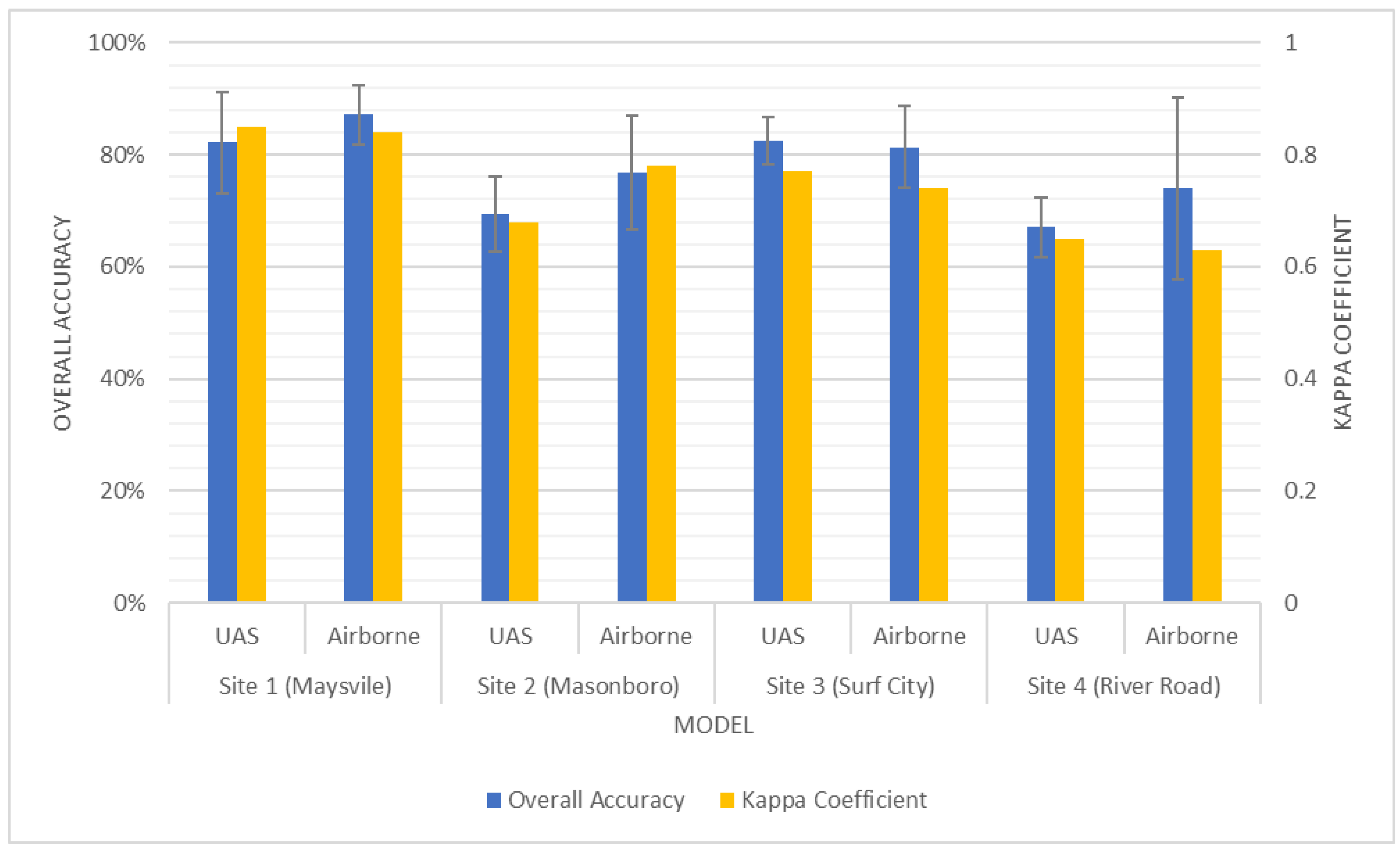
3.1. Wetland Classification Model

We assessed two models for the variable combinations presented above at each of the four surveyed locations. Figure 7 shows the resulting model performance metrics including overall accuracy (OA), the standard deviation of the OA (SD), and kappa coefficient (k) for each site by model type (UAS vs. airborne). All overall accuracies were above 60% and all kappa values were above 0.6, which shows that all the classifications performed satisfactorily. The highest accuracies were at Maysville and Surf City (both above 80%) and lowest at Masonboro and River Road sites. River Road performed the worst and also has the most complex wetland habitats that ranged from estuarine at the mouth to a mix of freshwater forested wetlands further upstream. The averages of the OA and K for the airborne models were 79.80% and 0.75, which was slightly higher than those of UAS models of 75.29% and 0.74 respectively. In addition, the average standard deviation was higher for the airborne models compared to the UAS at three out of the four sites tested except for Site 1 at Maysville (Figure S3). Specific metrics for class-level sensitivity and specificity are reported in Table S2.

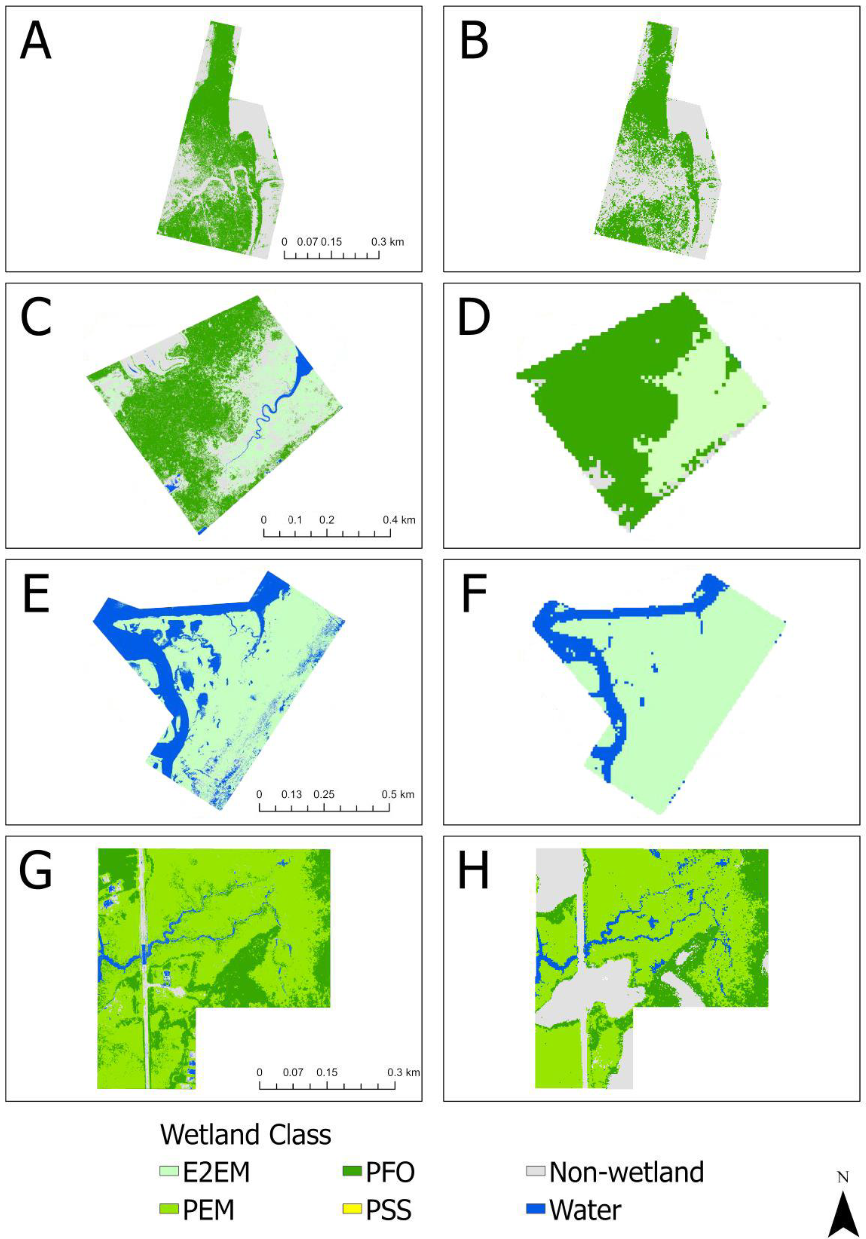
3.2. Classification Maps

We used the resulting models to create the wetland classification maps for each site (Figure S4). Figure 8 shows the total of eight resulting wetland maps: maps on the left side (Figure 9A,C,G,E) represent UAS models, and maps on the right side (Figure 8B,D,F,H) show the final classification output for airborne models. Since the UAS models were parameterized with hyperspatial LiDAR data, UAS model maps show more precise and detailed topography than the airborne model maps.
For Site 1 at Maysville NC, both the UAS (Figure 8A) and airborne (Figure 8B) models misclassified the water/hydrologic feature areas under the thick forest, with no actual detection of a water class. This was likely largely due to the fact that the water feature was mostly covered by the tree canopy during the survey, and LiDAR returns over water are null. Even though the UAS model could not classify the area as water class, it shows a clear delineation of the creek outline compared to the airborne model.
At Masonboro island (Site 2), flown during low tide conditions to capture the largest spatial extent of emergent wetland (saltmarsh) vegetation, the UAS-derived model shows a better delineation of the emergent wetlands than the airborne model map due to the spatial resolution differences (Figure 8C,D), despite the fact that the airborne model had higher OA than the UAS model. The UAS model identified detailed water extents, including the drainage channels and back-barrier features. However, both models underestimated non-wetland areas (mostly beach and beach dunes) at this location, despite the fact that the dunes are largely vegetated and should theoretically be therefore picked up in the multispectral data (although vegetation was largely senescent in the month of December).
The two models for site 3 (Surf City) show drastic differences between the UAS and airborne data in terms of class distribution and spatial resolution. This site is characterized primarily by estuarine emergent wetlands (E2EM) in almost equal proportion to water and non-wetland classes and has experienced large changes in land cover since the acquisition of the airborne LiDAR data. Although a PSS class was not classified in the UAS model (Figure 8E), the map shows the different kinds of wetland delineated. The airborne model (Figure 8F) overgeneralized the outputs with the classification map of just water and non-wetland classes, where there should be E2EM and PFO classes as indicated by both the NWI data and our ground reference data.
Finally, both models for Site 4 (River Road, Wilmington, NC, USA) show well-delineated classification maps and good overall and class accuracies. Due to the lower resolution of the airborne model map (Figure 8H), the map shows less precise wetland delineation extents than the UAS model map (Figure 9G). Although the UAS model shows higher overall accuracy and more detailed class boundaries, they overestimated the extent of the palustrine forested (PFO) class around the non-wetland area.

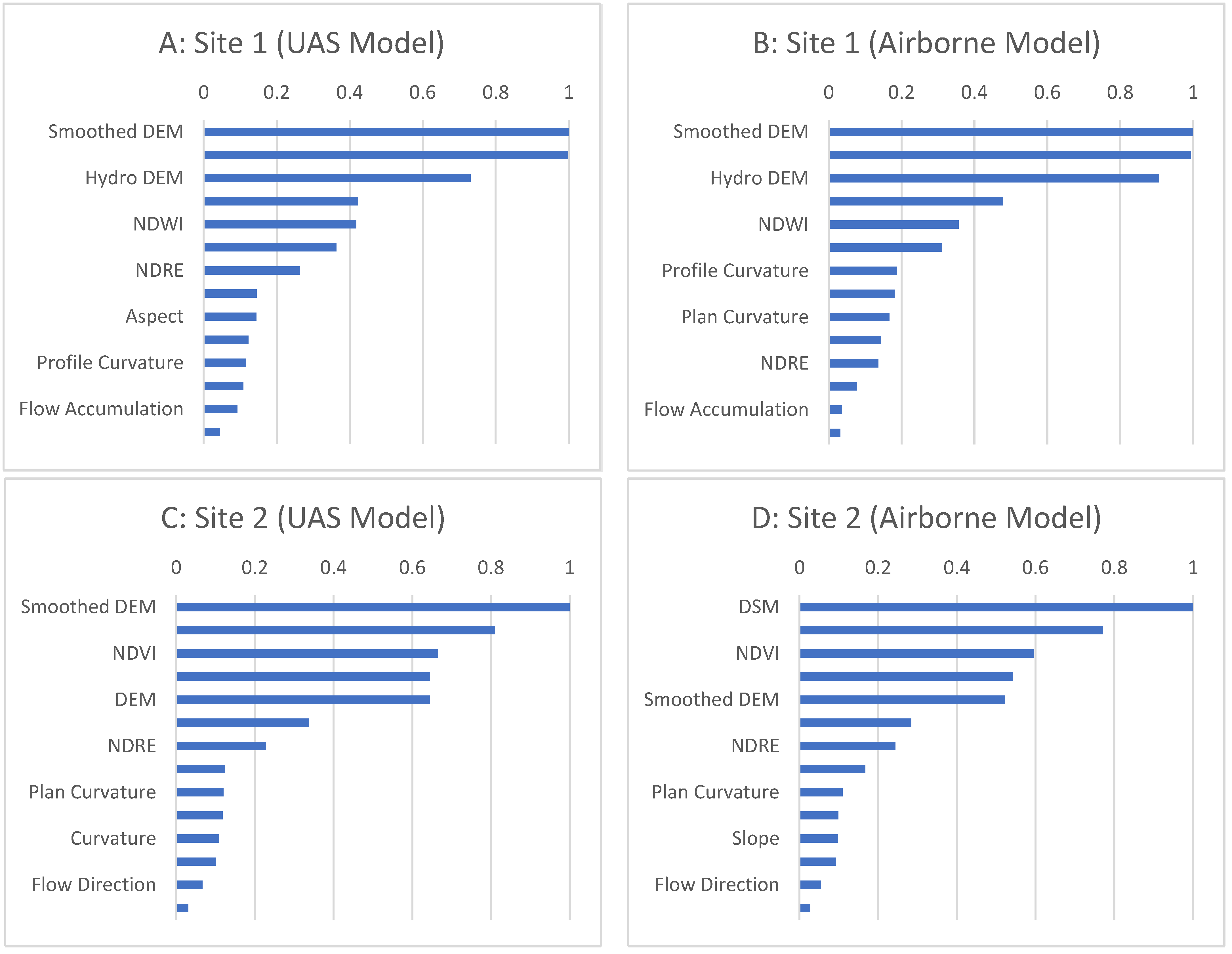
3.3. Variable Importance Classification

The scaled variable importance plots for all sites considered the role of all fourteen predictor variables and show that, among the topographic and vegetation index predictors considered in predicting forested wetlands, the LiDAR-derived topographic derivatives are ranked highest (Figure 9, left panels for the UAS models and right panels for the airborne models). For Site 1 (Maysville, NC, USA) for instance, both variable importance plots show the same top five variables: Smoothed DEM, DEM, Hydro DEM, NDVI, and NDWI. Slightly different combinations of those same top five variables are also top predictors for the UAS and airborne models at the estuarine island site (site 2 at Masonboro Island). Flow accumulation and flow direction are the least important variables for all the models for predicting wetland type and location in this low-lying gradient of wetlands characterized by small topographic variations, and are therefore not critical variables to include in future wetland classification models in this region.

4. Discussion

4.1. Model Performance

The main goal of this research was to ascertain the effectiveness of using hyperspatial UAS-collected LiDAR and multispectral data for coastal mapping and delineations. We lay out a clear methodology for data collection and reproducible pre-processing workflows using best practices similar to those presented in Guan et al. 2022, but we significantly extend this work by presenting UAS LiDAR collection and processing workflows identified as the next frontier in UAS research for coastal mapping and monitoring [35]. We contribute to extending the science and application of UAS data in mapping and monitoring coastal environments by providing detailed guidance on mission planning and implementation to optimally acquire vegetation data [36,37].
We then quantitatively compare model performance metrics (overall accuracies, standard deviation of accuracies from the sub-folds, kappa coefficients, and respective class sensitivities and specificities) and model prediction maps created by the hyperspatial UAS LiDAR (Quanergy M8) and the non-hyperspatial airborne LiDAR (QL2) and the UAS-collected multispectral data to determine the relative performance of these datasets for wetland delineation and classification. We summarize our findings into two main categories that we discuss below. As expected, we determine that models derived from hyperspatial UAS-collected LiDAR and multispectral datasets showed better performance than those parameterized with airborne-collected LiDAR data, despite the temporal discrepancy between the QL2 LiDAR and ground reference habitat field data, especially in terms of the accuracy of map precision (wetland delineation). Yet, both UAS and airborne-LiDAR parameterized models show comparative classification accuracies, and UAS LiDAR is most useful when temporally flexible mapping is needed. This applied to all four study sites included in this analysis except for Site 1 at Maysville, where we were only able to collect a relatively small number of habitat ground reference training data, but which is handled well be our ML classifier [38,39]. Using the habitat sampling data for model training and validation allowed us to produce classification maps with high precision from the UAS models; however, adding more habitat sample data would improve not only the classification maps but also the overall accuracies and the standard deviation. The difference in class-level specificity and sensitivity and the quality of the prediction maps depend on the LiDAR dataset used and the spatial resolution of the map. The average pixel size of UAS models and airborne models for all the sites was on average 0.3m and 6.3 m, respectively (Table S1). Thus, the results of our prediction maps showed more precise wetland class extents given the hyperspatial nature and temporally congruent nature of the UAS LiDAR data (2020–2021) relative to the airborne missions, and that sampling several distinct locations can provide useful data across sites [40].
An important contribution we make in line with emerging trends identified in Morgan et al. 2022 [36] is the application of fused multi-source UAS data to map distinct vegetation types that are inherently difficult to map in the absence of 3-dimensional data, such as forested and shrub scrub wetland types that characterize much of the US Coastal Plains. To map each type of wetland, the airborne and UAS LiDAR performed equally well for E2EM (estuarine intertidal emergent), PFO (palustrine forested), and PEM (palustrine emergent), but the UAS LiDAR was superior for the PSS (palustrine scrub shrub) wetland type (Table 7). This shows that for more structurally complex wetland types (PSS), UAS hyperspatial LiDAR data is much more advantageous given the multiple laser returns that can help map the vertical structure of these wetland types that are so common throughout the southeastern USA. Therefore, given that the main drawbacks of airborne LiDAR are poor temporal revisit and comparatively poorer spatial resolutions, the UAS LiDAR has proved to be highly accurate for wetland classification and useful on an as-needed basis, such as a post event or emergency, or further in combination with other active remote sensing datasets [41]. Hyperspatial UAS data can be utilized as ancillary or complementary datasets when conducting wetland research as they provide important information to fill gaps between habitat data collection and airborne or even satellite-based collections [36].
Overall, we show that for more structurally complex wetland types (such as the palustrine scrub shrub), UAS hyperspatial LiDAR data performs better and is much more advantageous to use in delineation and classification models given the multiple laser returns that can help map the vertical structure of these wetland types.
The second research objective was to find out the important variables that help classify the Coastal Plain wetlands and that capture the characteristics of the study areas. Elevation variables (DSM, DEM, smoothed DEM, and hydro-condition DEM) and vegetation indices (NDVI, NDRE, and NDWI) were consistently ranked within the top five, similar to work by Wen and Hughes 2020 [26]. Hydrogeomorphological variables such as flow direction and flow accumulation were ranked the least important, primarily due to the fact that the D8 flow calculation method is less effective in flat coastal environments, necessitating the development of alternative hydrologic variables [42,43]. High spatial resolution UAS-derived vegetation indices such as NDVI (or NDWI where surface water is present) are likewise the most important predictors of wetland type and condition. This finding is in line with wetland remote sensing literature that has found that, when it comes to optical bands that can be used for wetland classification, the red-edge and near-infrared bands perform best [38].

4.2. Challenges, Limitations, and Future Directions

In order to produce comparisons of the UAS and QL2 LiDAR data for creating topographic derivatives, we tested out a tessellation approach to generalize the data into smaller areas for direct comparisons and to reduce the computational intensity of pixel-based random forest models. One of the main challenges of working with hyperspatial LiDAR data is the computational load produced by pixel-based classification approaches despite the relatively small spatial extents of our study sites. This challenge was successfully addressed by using an R package dedicated to working with big data [26].
The main limitation of this research is the size and availability of training and validation data, which was made difficult by the topography, ground cover, and general impenetrability of the areas we surveyed. Collecting or creating additional habitat sampling data that is more evenly distributed across the various wetland classes would help ensure more balanced representation across study areas [39]. Additionally, separating non-wetland areas from one all-encompassing class into grass, bare, or tree-dominated classes would further improve model performance and increase class separability [37]. Additionally, additional predictor variables can be tested, including vertical canopy information such as a topographic position index or canopy height or density models [21,23]. More complex topographic indices, such as a topographic wetness index, soil-topographic wetness index, or a depth-to-water index, can also be tested for coastal plain low-gradient regions where more standard topo-hydrologic variables (flow direction or flow accumulation) performed very poorly [23,43]. Lastly, different machine learning classifications can be tested to compare the model performance, such as ensemble methods that introduce boosting and more adaptive learning algorithms [26].

5. Conclusion

This study evaluated the potential of hyperspatial UAS-collected LiDAR data relative to airborne-collected LiDAR data integrated with multispectral and in situ habitat samples to map and predict the extent, location, and wetland types along a North Carolina Coastal Plains ecosystem gradient. We document not only efficient and reproducible data collection and processing workflows for LiDAR data acquisition from a UAS, but also a transferable approach to create wetland random forest delineation and classification models that outperform NWI delineations.
We conclude that UAS-based remote sensing technologies can produce very powerful datasets that are useful for wetland research. This work offers a starting point for the enhancement of wetland delineation and classification models focused on forested wetlands that were previously difficult to map prior to UAS-based LiDAR datasets being available. By providing a direct comparison of the UAS LiDAR data relative to airborne data, despite the temporal and point density differences, we show that UAS-collected LiDAR is reliable and can continue to be explored and used in coastal research. Further work should continue to investigate the capabilities of hyperspatial LiDAR data in classifying forested wetlands using different predictors and improved response variables optimized for low-gradient coastal systems.

Supplementary Materials

The following supporting information can be downloaded at: https://www.mdpi.com/article/10.3390/drones6100268/s1, Table S1: The RMSEz values of all collected LiDAR data, Figure S1: A workflow diagram, Figure S2: Figures of wetland categories, Figure S3: The standard deviation of the overall accuracy for each site (for each of the 5-fold cross-validated models), Table S2: Specific metrics for class-level sensitivity and specificity and Figure S4: Three-dimensional visualizations of the four sites are provided as Supplementary Material.

Author Contributions

Conceptualization, N.G.P.; methodology, N.G.P., A.M. and J.N.H.; software, N.G.P., A.M.; validation, A.M., N.G.P.; formal analysis, A.M., N.G.P., C.C. and Y.W.; investigation, N.G.P., J.N.H.; resources, N.G.P.; data curation, A.M., N.G.P., C.C. and Y.W.; writing—original draft preparation, A.M., N.G.P.; writing—review and editing, N.G.P.; visualization, A.M.; supervision, N.G.P.; project administration, N.G.P.; funding acquisition, N.G.P., J.N.H. All authors have read and agreed to the published version of the manuscript.

Funding

This research was funded by the North Carolina Department of Transportation, contract number RP 2020–04 awarded to Narcisa Pricope and Joanne Halls in the Earth and Ocean Sciences Department at the University of North Carolina Wilmington.

Institutional Review Board Statement

Not applicable.

Informed Consent Statement

Not applicable.

Data Availability Statement

Any of the datasets and codes used in this publication can be made available upon request.

Acknowledgments

We want to thank the North Carolina Department of Transportation for facilitating and funding this research and extend a special thanks to Morgan Weatherford and Wes Cartner for their roles in this project. We would also like to thank the following companies and individuals for their contributions to this research: Lonnie Sears (PLS, CMS-UAS) and Pat Davis (PLS) of eGPS Solutions for providing the DJI Matrice 600 Pro and initial equipment training. We would also like to extend a special thank you to Kerry Mapes and graduate students Jesse Scopa, Carter Eckhardt, James Giddens, and Britton Baxley for assistance during field data collection for this project.

Conflicts of Interest

The authors declare no conflict of interest. The funders had no role in the design of the study; in the collection, analyses, or interpretation of data; in the writing of the manuscript; or in the decision to publish the results.

References

  1. EPA. America’s Wetlands: Our Vital Link Between Land and Water. In NSCEP; U.S. Environmental Protection Agency, Office of Water, Office of Wetlands, Oceans and Watersheds: Washington, DC, USA, 1995; pp. 1–16. [Google Scholar]
  2. Woodward, R.T.; Wui, Y.S. The economic value of wetland services: A meta-analysis. Ecol. Econ. 2001, 37, 257–270. [Google Scholar] [CrossRef]
  3. Richardson, C.J. Ecological functions and human values in wetlands: A framework for assessing forestry impacts. Wetlands 1994, 14, 1–9. [Google Scholar] [CrossRef]
  4. EPA. Coastal Wetlands Initiative: Mid-Atlantic Review. Available online: https://www.epa.gov/wetlands/epas-efforts-coastal-wetlands-initiative-0 (accessed on 22 April 2022).
  5. Hu, S.J.; Niu, Z.G.; Chen, Y.F.; Li, L.F.; Zhang, H.Y. Global wetlands: Potential distribution, wetland loss, and status. Sci. Total Environ. 2017, 586, 319–327. [Google Scholar] [CrossRef] [PubMed]
  6. Davidson, N.C. How much wetland has the world lost? Long-term and recent trends in global wetland area. Mar. Freshw. Res. 2014, 65, 934–941. [Google Scholar] [CrossRef]
  7. Dahl, T.E.; Johnson, C.E.; Frayer, W.E. Wetlands Status and Trends in the Conterminous United States Mid-1970′s to Mid-1980′s; United States Fish and Wildlife Service: Washington, DC, USA, 1991; Volume 28.
  8. Dah, T.E. Status and Trends of Wetlands in the Coastal Wetlands of the Continuous United States 2004 to 2009; U.S. Department of the Interior; Fish and Wildlife Service: Washington, DC, USA, 2013; p. 108.
  9. Rodriguez, C.F.; Becares, E.; Fernandez-Alaez, M.; Fernandez-Alaez, C. Loss of diversity and degradation of wetlands as a result of introducing exotic crayfish. Biol. Invasions 2005, 7, 75–85. [Google Scholar] [CrossRef]
  10. Sutter, L. DCM Wetland Mapping in Coastal North Carolina. In The North Carolina Department of Environment and Natural Resources Pursuant to the United States Environmental Protection Agency Award No. 994548-94-5; North Carolina Division of Coastal Management: Morehead City, NC, USA, 1999. [Google Scholar]
  11. Gale, S. National Wetlands Inventory (NWI) Accuracy in North Carolina; USEPA Multipurpose Grant AA-01D03020; NC Department of Environmental Quality Division of Water Resources: Raleigh, NC, USA, 2021.
  12. Jeziorska, J. UAS for Wetland Mapping and Hydrological Modeling. Remote Sens. 2019, 11, 1997. [Google Scholar] [CrossRef]
  13. Pricope, N.G.; Halls, J.N.; Mapes, K.L.; Baxley, J.B.; Wu, J.J. Quantitative Comparison of UAS-Borne LiDAR Systems for High-Resolution Forested Wetland Mapping. Sensors 2020, 20, 4453. [Google Scholar] [CrossRef]
  14. Abeysinghe, T.; Milas, A.S.; Arend, K.; Hohman, B.; Reil, P.; Gregory, A.; Vazquez-Ortega, A. Mapping Invasive Phragmites australis in the Old Woman Creek Estuary Using UAV Remote Sensing and Machine Learning Classifiers. Remote Sens. 2019, 11, 1380. [Google Scholar] [CrossRef]
  15. Guo, M.; Li, J.; Sheng, C.L.; Xu, J.W.; Wu, L. A Review of Wetland Remote Sensing. Sensors 2017, 17, 777. [Google Scholar] [CrossRef]
  16. Millard, K.; Richardson, M. Wetland mapping with LiDAR derivatives, SAR polarimetric decompositions, and LiDAR-SAR fusion using a random forest classifier. Can. J. Remote Sens. 2013, 39, 290–307. [Google Scholar] [CrossRef]
  17. Tian, S.H.; Zhang, X.F.; Tian, J.; Sun, Q. Random Forest Classification of Wetland Landcovers from Multi-Sensor Data in the Arid Region of Xinjiang, China. Remote Sens. 2016, 8, 954. [Google Scholar] [CrossRef]
  18. Kuleli, T.; Guneroglu, A.; Karsli, F.; Dihkan, M. Automatic detection of shoreline change on coastal Ramsar wetlands of Turkey. Ocean Eng. 2011, 38, 1141–1149. [Google Scholar] [CrossRef]
  19. Lubczonek, J.; Kazimierski, W.; Zaniewicz, G.; Lacka, M. Methodology for combining data acquired by unmanned surface and aerial vehicles to create digital bathymetric models in shallow and ultra-shallow waters. Remote Sens. 2021, 14, 105. [Google Scholar] [CrossRef]
  20. Specht, M.; Specht, C.; Lewicka, O.; Makar, A.; Burdziakowski, P.; Dąbrowski, P. Study on the Coastline Evolution in Sopot (2008–2018) Based on Landsat Satellite Imagery. J. Mar. Sci. Eng. 2020, 8, 464. [Google Scholar] [CrossRef]
  21. Rapinel, S.; Hubert-Moy, L.; Clement, B. Combined use of LiDAR data and multispectral earth observation imagery for wetland habitat mapping. Int. J. Appl. Earth Obs. Geoinf. 2015, 37, 56–64. [Google Scholar] [CrossRef]
  22. Chust, G.; Galparsoro, I.; Borja, A.; Franco, J.; Uriarte, A. Coastal and estuarine habitat mapping, using LIDAR height and intensity and multi-spectral imagery. Estuar. Coast. Shelf Sci. 2008, 78, 633–643. [Google Scholar] [CrossRef]
  23. Wang, S.-G.; Deng, J.; Chen, M.; Weatherford, M.; Paugh, L. Random Forest Classification and Automation for Wetland Identification based on DEM Derivatives. In Proceedings of the 2015 ICOET (International Conference on Ecology and Transportation), Raleigh, NC, USA, 20–24 September 2015; pp. 402–408. [Google Scholar]
  24. O’Neil, G.L.; Saby, L.; Band, L.E.; Goodall, J.L. Effects of LiDAR DEM smoothing and conditioning techniques on a topography-based wetland identification model. Water Resour. Res. 2019, 55, 4343–4363. [Google Scholar] [CrossRef]
  25. Mohri, M.; Rostamizadeh, A.; Talwalkar, A. Foundations of Machine Learning; MIT Press: Cambridge, MA, USA, 2018. [Google Scholar]
  26. Wen, L.; Hughes, M. Coastal wetland mapping using ensemble learning algorithms: A comparative study of bagging, boosting and stacking techniques. Remote Sens. 2020, 12, 1683. [Google Scholar] [CrossRef]
  27. Cowardin, L.M.; Carter, V.; Golet, F.C.; LaRoe, E.T. Classification of Wetlands and Deepwater Habitats of the United States; Fish and Wildlife Service, US Department of the Interior: Washington, DC, USA, 1979.
  28. Fear, J.A. Comprehensive Site Profile for the North Carolina National Estuarine Research Reserve; The North Carolina National Estuarine Research Reserve: Apex, NC, USA, 2008. [Google Scholar]
  29. Anders, N.; Valente, J.; Masselink, R.; Keesstra, S. Comparing filtering techniques for removing vegetation from UAV-based photogrammetric point clouds. Drones 2019, 3, 61. [Google Scholar] [CrossRef]
  30. Hashimoto, K.; Shimozono, T.; Matsuba, Y.; Okabe, T. Unmanned aerial vehicle depth inversion to monitor river-mouth bar dynamics. Remote Sens. 2021, 13, 412. [Google Scholar] [CrossRef]
  31. Cai, S.S.; Zhang, W.M.; Liang, X.L.; Wan, P.; Qi, J.B.; Yu, S.S.; Yan, G.J.; Shao, J. Filtering Airborne LiDAR Data Through Complementary Cloth Simulation and Progressive TIN Densification Filters. Remote Sens. 2019, 11, 1037. [Google Scholar] [CrossRef]
  32. Aiello, S.; Eckstrand, E.; Fu, A.; Landry, M.; Aboyoun, P. Machine Learning with R and H2O. 2018. Available online: http://h2o.ai/resources/ (accessed on 6 May 2022).
  33. R Core Team. R: A Language and Environment for Statistical Computing. The R Project for Statistical Computing. 2020. Available online: https://www.r-project.org/ (accessed on 6 May 2022).
  34. Berrar, D. Cross-Validation. Encycl. Bioinform. Comput. Biol. 2019, 1, 542–545. [Google Scholar] [CrossRef]
  35. Guan, S.; Sirianni, H.; Wang, G.; Zhu, Z. sUAS Monitoring of Coastal Environments: A Review of Best Practices from Field to Lab. Drones 2022, 6, 142. [Google Scholar] [CrossRef]
  36. Morgan, G.R.; Hodgson, M.E.; Wang, C.; Schill, S.R. Unmanned aerial remote sensing of coastal vegetation: A review. Drones 2022, 6, 142. [Google Scholar] [CrossRef]
  37. Dronova, I.; Kislik, C.; Dinh, Z.; Kelly, M. A review of unoccupied aerial vehicle use in wetland applications: Emerging opportunities in approach, technology, and data. Drones 2021, 5, 45. [Google Scholar] [CrossRef]
  38. Mahdavi, S.; Salehi, B.; Granger, J.; Amani, M.; Brisco, B.; Huang, W. Remote sensing for wetland classification: A comprehensive review. GIScience Remote Sens. 2018, 55, 623–658. [Google Scholar] [CrossRef]
  39. Lei, G.; Li, A.; Bian, J.; Yan, H.; Zhang, L.; Zhang, Z.; Nan, X. OIC-MCE: A practical land cover mapping approach for limited samples based on multiple classifier ensemble and iterative classification. Remote Sens. 2020, 12, 987. [Google Scholar] [CrossRef]
  40. Belluco, E.; Camuffo, M.; Ferrari, S.; Modenese, L.; Silvestri, S.; Marani, A.; Marani, M. Mapping salt-marsh vegetation by multispectral and hyperspectral remote sensing. Remote Sens. Environ. 2006, 105, 54–67. [Google Scholar] [CrossRef]
  41. Sun, S.; Zhang, Y.; Song, Z.; Chen, B.; Zhang, Y.; Yuan, W.; Chen, C.; Chen, W.; Ran, X.; Wang, Y. Mapping coastal wetlands of the Bohai Rim at a spatial resolution of 10 M using multiple open-access satellite data and terrain indices. Remote Sens. 2020, 12, 4114. [Google Scholar] [CrossRef]
  42. Wilson, J.P.; Lam, C.S.; Deng, Y. Comparison of the performance of flow-routing algorithms used in GIS-based hydrologic analysis. Hydrol. Processes Int. J. 2007, 21, 1026–1044. [Google Scholar] [CrossRef]
  43. O’Neil, G.L.; Goodall, J.L.; Watson, L.T. Evaluating the potential for site-specific modification of LiDAR DEM derivatives to improve environmental planning-scale wetland identification using Random Forest classification. J. Hydrol. 2018, 559, 192–208. [Google Scholar] [CrossRef]
Figure 1. National Wetlands Inventory (NWI) source image year of acquisition/creation in North Carolina, USA.
Drones 06 00268 g001
Figure 2. The four study areas in southeastern North Carolina, USA, dominated by four distinct types of wetland classes. The classification layers used for the study sites were obtained from the National Wetland Inventory dataset.
Drones 06 00268 g002
Figure 3. The DJI Matrice 600 Pro (M-600 Pro, manufactured by DJI, Beijing, China) equipped with a LiDAR USA Quanergy M8 LiDAR sensor was used in the study (photo by N. Pricope). The M600 Pro is a six-armed rotocoptor with an onboard A3 Pro flight controller and Lightbridge 2 HD transmission system capable of reaching a maximum speed of 65 kph in windless conditions.
Drones 06 00268 g003
Figure 4. Example flight mission design for Site 3 (Masonboro Island, NC, USA) showing the area of interest for a collection, the LiDAR flight paths generated in ArcGIS Pro and uploaded to Ground Station Pro, and the ground control points (GCPs) used for georeferencing. The fixed wing multispectral flights covered the exact same area of interest and were implemented in eMotion 3.
Drones 06 00268 g004
Figure 5. Workflow overview. Raw Quanergy LiDAR and raw multispectral data were preprocessed first, and all the input data were processed into one raster stack for random forest analysis. Final maps, model evaluations, and variable importance plots were produced from the RF models in R.
Drones 06 00268 g005
Figure 6. Composition of the two raster stacks used in the wetland prediction model: one for the hyperspatial Quanergy data and another for the QL2 airborne LiDAR data. The vegetation indices were derived from the UAS-collected multispectral data for both sets of models.
Drones 06 00268 g006
Figure 7. Model overall accuracy (OA), the standard deviation (SD), and kappa coefficient (k) for each site.
Drones 06 00268 g007
Figure 8. The resulting classification maps, UAS models on the left and airborne models on the right. The maps represent wetland models of the UAS (A) and airborne (B) for Site 1 (Maysville), the UAS (C) and airborne (D) for Site 2 (Surf City), the UAS (E) and airborne (F) for Site 3 (Masonboro Island), and the UAS (G) and airborne (H) for Site 4 (River Road).
Drones 06 00268 g008
Figure 9. The resulting scaled variable importance plots. Site 1 (Maysville), UAS model (A) and the airborne model (B). For Site 1, UAS model (A) and the airborne model (B). Site 2 (Masonboro), UAS model (C) and the airborne model (D). Site 3 (Surf City), UAS model (E) and the airborne model (F). Site 4 (River Road, Wilmington, NC), UAS model (G) and the airborne model (H).
Drones 06 00268 g009aDrones 06 00268 g009b
Table 1. Wetland types, NWI codes, and descriptions characteristic of the study area. Each wetland type is described as the following class codes in the table.
Wetland TypesWetland CodesDescriptions
Estuarine Intertidal EmergentE2EMThe estuarine system consists of deep-water tidal habitats and adjacent tidal wetlands that are usually semi-enclosed by land but have open access to the open ocean. This system is characterized by the presence of intertidal and emergent vegetation.
Palustrine ForestPFOThe palustrine system includes inland, nontidal wetlands characterized by the presence of forest.
Palustrine EmergentPEMThe palustrine system includes inland, nontidal wetlands characterized by the presence of emergent vegetation.
Palustrine Scrub-ShrubPSSThe palustrine system includes inland, nontidal wetlands characterized by the presence of scrub-shrub.
Table 2. Wetland class distribution per site determined using the most recent NWI data. Each class code is described as the following class codes; E2EM: estuarine intertidal emergent, PFO: palustrine forest, PEM: palustrine emergent, and PSS: palustrine scrub-shrub.
Class CodeSite 1Site 2Site 3Site 4
E2EM-28.00%46.86%-
PFO40.02%62.04%-9.00%
PEM---55.65%
PSS-0.58%--
Water0.80%1.15%27.17%1.18%
Non-wetland59.17%8.23%25.97%34.17%
Total Acreage43.8078.28109.9854.34
Table 3. Fieldwork was conducted between October 2020 and January 2021. UAS LiDAR point cloud data, UAS high-resolution multispectral image data, and ground-based habitat reference data were collected in the field at four sites.
Site NamesFieldwork Dates
Site 1: Maysville22 January 2021
Site 2: Surf City6 November 2020
Site 3: Masonboro11 December 2020
Site 4: River Road3 October 2020
Table 4. UAS (Quanergy M8) and statewide airborne (QL2)-mounted LiDAR scanners and their respective specifications. Hyperspatial LiDAR data were collected using the Quanergy sensor in the field while Leica and Pegasus sensors collected LiDAR point clouds processed into the QL2 LiDAR.
ParametersQuanergy M8 CoreLeica ALS70HPPegasus HA500
PlatformUASAircraftAircraft
Wavelength905 nm1064 nm1064 nm
Frame Rate5–20 Hz120–200 Hz0–140 Hz
FOV (degree)Horizontal: 360°,
Vertical: 20° (+3°/−17°)
0–750–75
Range [m]1–150200–3500150–5000
Range accuracy [cm]<3 (1σ at 50 m)7–16<5–20
Returns3unlimited4
Weight [kg]0.95965
Table 5. The characteristics of the multispectral Parrot Sequoia sensor aboard a SenseFly eBee Plus RTK UAS.
Parrot Sequoia+
Multispectral BandsGreen (550 nm ± 40 nm)
Red (660 nm ± 40 nm)
Red edge (735 nm ± 10 nm)
Near-infrared (790 nm ± 40 nm)
Single-band resolution1.2 MP
1280 × 960 px (4:3)
Single-Band FOVHFOV: 62°
VFOV: 49°
DFOV: 74°
Table 6. Names and description of the predictor and response variables derived from the LiDAR and multispectral data.
Data InputDefinition
DSMMax height elevation (including vegetation and artificial objects) in meters
DEMGround elevation (vegetation and artificial objects removed) in meters
Smoothed DEMSmoothing is used to smooth DEMs to remove the elevation changes that are too small to indicate features of interest (i.e., microtopographic noise), which are ubiquitous in high-resolution DEMs. Smoothing method: Perona–Malik [24]
Hydro-condition DEM
(Hydro DEM)
Hydro-conditioning resolves topographic depressions before modeling flow paths
AspectCompass direction of the steepest downhill gradient
SlopeThe steepness at each cell of a raster surface
CurvatureThe slope of the slope
Plan CurvatureCurvature on horizontal (x) direction
Profile CurvatureCurvature on vertical (y) direction
Flow DirectionThe direction of flow from every pixel in the raster
Flow AccumulationAccumulated flow is the accumulated weight of all cells flowing into each downslope cell in the output raster
NDVIIt quantifies photosynthetically active vegetation (Equation (1)). The values range from −1 to 1.
NDREIt quantifies levels of chlorophyll content. High values indicate photosynthetically active plants, with bare soil having low values (Equation (2)). The values range from −1 to 1.
NDWIIt estimates the leaf water content at canopy level (Equation (3)). The values range from −1 to 1.
Habitat TypeIt contains the wetland type that was verified either in the field or through on-screen analysis. This variable is used as a response.
Table 7. Class sensitivity and specificity metrics for all models across the different types of wetland systems captured in our surveys (QL2+MS indicates models parameterized with the airborne LiDAR and UAS multispectral data while Quanergy + MS denotes models parameterized with the UAS LiDAR and multispectral).
WETLAND TYPECLASSIFICATION METHODSENSITIVITYSPECIFICITYSITE
E2EMMS88%84%Surf City
MS86%90%Masonboro
QL294%97%Surf City
QL293%94%Masonboro
Quanergy94%95%Surf City
Quanergy92%95%Masonboro
QL2 + MS96%98%Surf City
QL2 + MS94%95%Masonboro
Quanergy + MS95%95%Surf City
Quanergy + MS94%96%Masonboro
PFOMS52%85%Maysville
MS86%77%Surf City
QL266%98%RR
QL295%93%Maysville
QL297%88%Surf City
Quanergy41%98%RR
Quanergy94%92%Maysville
Quanergy95%80%Surf City
QL2 + MS68%98%RR
QL2 + MS96%94%Maysville
QL2 + MS98%89%Surf City
Quanergy + MS42%98%RR
Quanergy + MS95%93%Maysville
Quanergy + MS95%82%Surf City
PEMMS94%48%RR
QL297%87%RR
Quanergy96%73%RR
QL2 + MS97%88%RR
Quanergy + MS96%75%RR
PSSMS80%100%Surf City
QL252%100%Surf City
Quanergy80%100%Surf City
QL2 + MS80%100%Surf City
Quanergy + MS87%100%Surf City
Publisher’s Note: MDPI stays neutral with regard to jurisdictional claims in published maps and institutional affiliations.

