Fully Distributed Robust Formation Flying Control of Drones Swarm Based on Minimal Virtual Leader Information

Abstract

This paper studies the robust formation flying problem for a swarm of drones, which are modeled as uncertain second order systems. By making use of minimal virtual leader information, a fully distributed robust control scheme is proposed, which includes three parts. First, the output based adaptive distributed observer is adopted to recover the global flying path vector as well as the coefficients of the minimal polynomial of the system matrix of the virtual leader system for each drone based on neighboring information from the communication network. Second, based on the estimated minimal polynomial of the system matrix of the virtual leader system, an asymptotic internal model is conceived to deal with uncertain system parameters. Third, by combining the asymptotic internal model and a certainty equivalent dynamic state feedback control law, a local trajectory tracking controller is synthesized to solve the robust formation flying problem. Numerical simulations are provided to validate the proposed control scheme.

1. Introduction

Animal swarming behaviors are universal in nature, such as the flocking of birds [1] and schooling of fish [2]. As revealed by scientists, movement in formation may help the animal swarm to save energy and increase efficiency for long distance migration [3]. Inspired by these intriguing swarming behaviors of living creatures, formation control for various types of unmanned swarm systems has been widely investigated by both the control and robotic communities, such as ground mobile robots [4], unmanned aerial vehicles [5], and autonomous underwater vehicles [6], just to name a few. There are two key control objectives for formation control. On the one hand, all the individuals in the swarm should track some common reference path, and on the other hand, the individuals should keep the desired relative position/attitude with respect to each other so that the swarm system as a whole exhibits certain spacial configuration. Autonomous formation control is the foundation of many practical tasks for unmanned swarm systems, such as cooperative load transportation [7], area exploration and surveillance [8,9], and cooperative hunting [10].

Roughly speaking, the existing control strategies for the formation control of swarm systems fall into three categories, namely, the behavior-based strategy, the leader-follower strategy, and the virtual structure strategy [11,12,13]. For the behavior-based strategy, the basic task modules are named “motor schemas”, such as goal-searching, obstacle avoidance, and formation keeping. The control policy is determined by calculating the weighted sum of different motor schemas. A seminal work using behavior-based strategy was reported in [14]. Later, the behavior-based strategy was further developed in [15] by decomposing a complex formation maneuver into a sequence of sub-level maneuvers. Recently, a bio-inspired behavior-based swarm strategy was studied in [16] for environment exploration, which did not rely on complicated sensing or computation. In the leader-follower strategy, two individuals form a leader-follower pair and all the leader-follower pairs are linked together to form a leader-follower chain. Swarm formation is fulfilled by achieving relative position/attitude tracking for each leader-follower pair. Ref. [17] proved the stability of the leader-follower strategy-based control algorithms for mobile robots, and Ref. [18] removed the assumption on the acquisition of absolute individuals’ positions for formation control by utilizing a position estimator. The virtual structure strategy defines the spacial configuration of formation through the relative position/attitude between each individual and a common motion trajectory, which is referred to as the virtual leader. In this way, no actual physical leader is required. Among the extensive results using the virtual structure strategy, Dong et. al. established a systematic control framework [19,20,21] for the distributed formation control of swarm systems. In these works, the information of the swarm system flow over a communication network, and each individual can only communicate with its neighboring individuals of the network topology. The control approach satisfying such communication constraint is called a distributed control [22,23,24,25]. By viewing the virtual leader of the virtual structure strategy as the exosystem, the distributed formation control problem can be treated in a concise and elegant way by the cooperative output regulation theory [26], which shows a unique advantage in simultaneously dealing with heterogeneous individual dynamics, unreliable communication networks, and system parameter uncertainties. Until now, there have been quite some efforts devoted to the application of the cooperative output regulation theory to the distributed formation problem [27,28,29,30,31,32,33,34,35,36]. A virtual error-based distributed internal model approach was proposed in [27], which could handle uncertain system parameters and unreliable communication network at the same time. Ref. [28] considered the case where the virtual leader was subject to an external input, and the state of the virtual leader was estimated by a distributed observer with a self-tuning gain. The case of multiple virtual leaders was investigated in [29], where all the individuals would converge to the convex set spanned by all the virtual leaders. In [30], a dynamic event-triggered communication mechanism was explored to reduce the communication cost. Ref. [31] extended the work of [27] from linear individual dynamics to nonlinear individual dynamics on the basis of non-smooth analysis and Lyapunov theory. Distributed filters were developed in [32] to deal with communication quantization and attacks. In certain application scenarios, cooperation and antagonism may coexist among the individuals, which gives rise to a signed communication graph. In such scenarios, bipartite formation problem is further pursued [33,34,35,36]. The case of multiple leaders was studied in [33,34], where the leaders in [33] had no external inputs, while the leaders in [34] were subject to external inputs. Moreover, actuator faults were investigated in [35], and the containment problem was tackled by the dual-terminal event-triggered output feedback control. Over the signed communication graph, a fixed-time adaptive distributed observer was proposed by [36] to solve the finite-time distributed bipartite tracking problem.

Based on the cooperative output regulation theory, in this paper, we further study the robust formation flying problem for a swarm of drones which are modeled as uncertain second order systems. By making use of minimal virtual leader information, as illustrated by Figure 1, a fully distributed robust control scheme is proposed, which includes three parts. To begin with, the output-based adaptive distributed observer is adopted to recover the global flying path vector as well as the coefficients of the minimal polynomial of the system matrix of the virtual leader system for each drone based on neighboring information from the communication network. Then, based on the estimated minimal polynomial of the system matrix of the virtual leader system, an asymptotic internal model is conceived to deal with uncertain system parameters. Finally, by combining the asymptotic internal model and a certainty equivalent dynamic state feedback control law, a local trajectory tracking controller is synthesized to solve the robust formation flying problem. To make the proposed control scheme feasible, the following three theoretical challenges have been overcome.

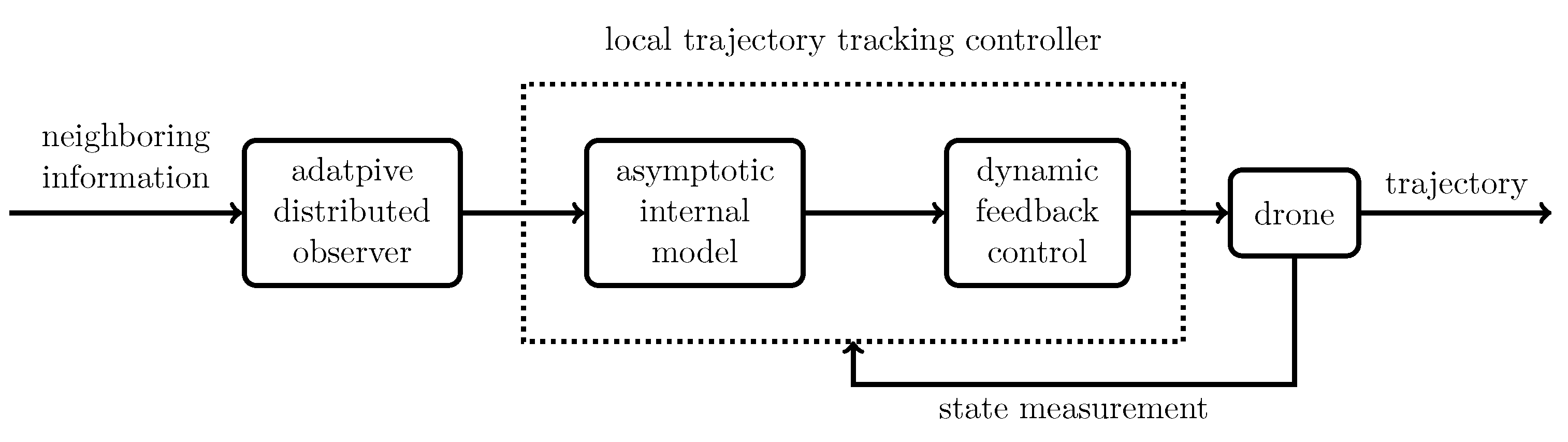
• The reference path for each drone is a composite of the global flying path vector and the local formation vector. As a result, to achieve local trajectory tracking, the asymptotic internal model should cover the generating modes of both the global flying path vector and the local formation vector. To this end, the minimal polynomials associated with the global and local reference vectors are multiplied together to obtain an integrated internal model, which covers the generating modes of both the global and local reference vectors.
• The controllability of the matrix pair of the internal model is a prerequisite for synthesizing the dynamic state feedback control. For the time-invariant internal model, the matrix pair can take any form. Meanwhile, since the asymptotic internal model conceived in this paper is time-varying, we have adopted the canonical controllable form for the matrix pair of the asymptotic internal model so that the time-varying system matrices of the augmented closed-loop system associated with the time-varying asymptotic internal model is controllable for all the time being.
• In the design of the dynamic state feedback control, the control gains should be properly assigned so that all the eigenvalues of the nominal closed-loop system will be placed at pre-specified locations in the complex plane. Though it is easy to conduct this eigenvalue placement procedure for time-invariant matrix pair, the same calculation for time-varying matrix pair might not be straightforward if the time-varying matrix pair is merely stabilizable. To thoroughly address this issue, in this paper, we have proposed a novel adaptive gain assignment method by solving the real-time algebraic Riccati equation to stabilize the time-varying closed-loop system.

In comparison with the existing results, the main contributions of this paper are summarized as follows.

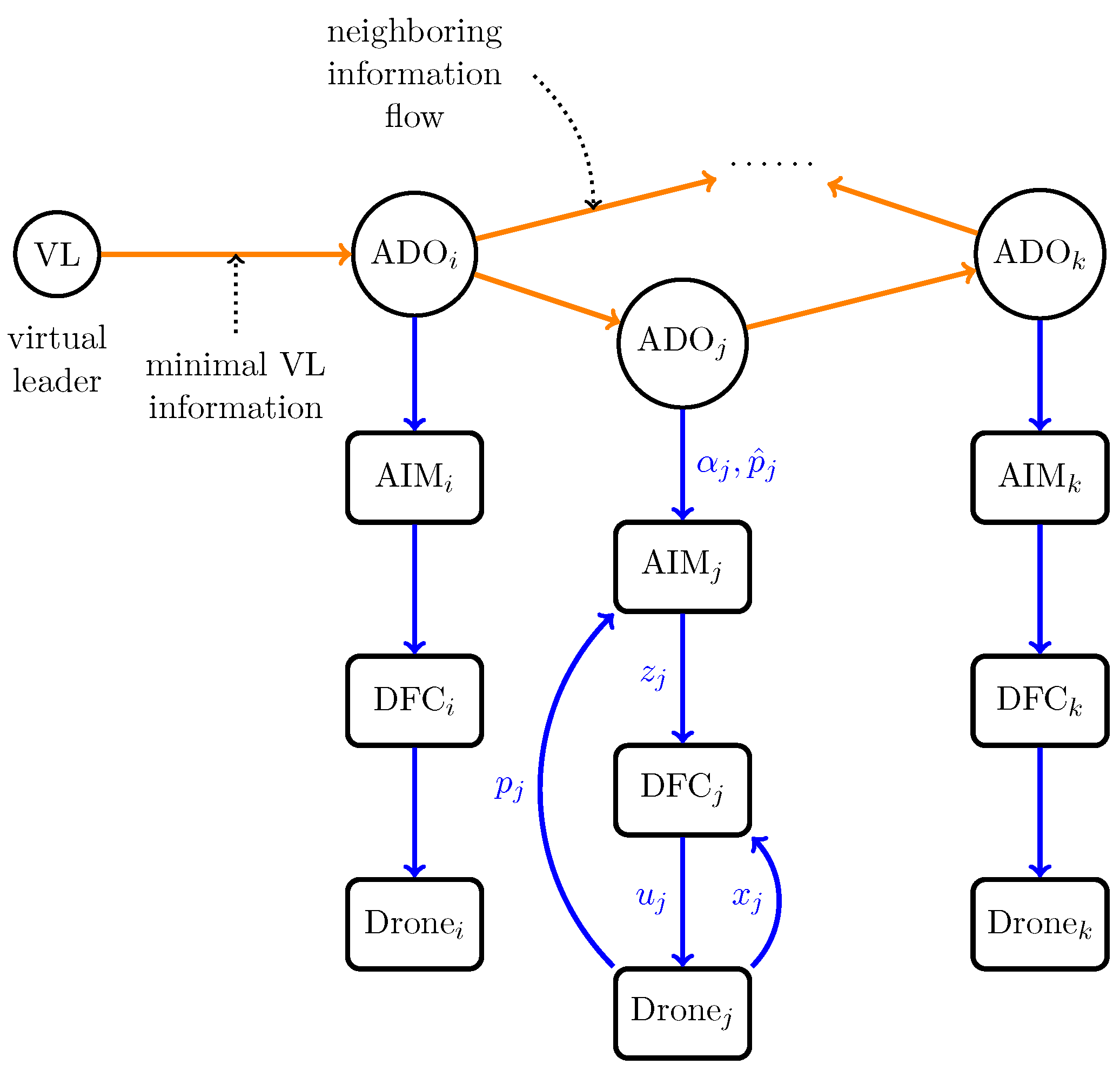
• The internal model approaches adopted in [27,31,32], and also in our previous work ([26], Chapter 10) required that full/partial information of the exosystem should be known to each individual in advance. Meanwhile, in this paper, the virtual leader which generates the global flying path vector is initially completely unknown to all the drones. The information of the virtual leader will be transmitted to each drone through the output feedback adaptive distributed observer proposed in [37]. Based on the estimated minimal polynomial of the system matrix of the virtual leader system, an asymptotic internal model is conceived to deal with system uncertainties.
• It is noteworthy that in [33,34,35,36], and also in our previous works ([26], Chapters 8 and 11) and [38], all the elements of the system matrices need to be recovered by various adaptive distributed observers. While, in this paper, by invoking the output-based adaptive distributed observer, much less system parameters need to be transmitted over the communication network, which drastically reduces the communication burden in comparison with the existing results.
• In [28,29,33,34,35,36,39,40], the individual models are free of parameter uncertainty. In contrast, in this paper, both the uncertain velocity damping matrix and the uncertain control gain matrix are taken into consideration for the second order drone models. To deal with system parameter uncertainties, we have resorted to the p-copy internal model approach [41], which is robust against moderate variations of system parameters around their nominal values.

The rest of this paper is organized as follows. Section 2 summarizes the notation and preliminary that will be used subsequently in this paper. The robust formation flying problem is described in Section 3. The main results of this paper are presented in Section 4. Numerical simulations are provided in Section 5 to validate the proposed control approach. Finally, Section 6 concludes this paper.

2. Notation and Preliminary

$\mathbb{R}$ and $\mathbb{C}$ denote the real and complex number field, respectively. ⊗ denotes the Kronecker product of matrices. $I_N$ denotes N-dimensional identity matrix. For $A_i\in {\mathbb{R}}^{m_i\times m_i}$, $i=1,\cdots ,M$, $\mathcal{D}(A_1,\cdots ,A_M)=\mathrm{block}\mathrm{diag}\{A_1,\cdots ,A_M\}$. For $x_i\in {\mathbb{R}}^{n_i}$, $i=1,\cdots ,N$, $col(x_1,\cdots ,x_N)={[x_1^T,\cdots ,x_N^T]}^T$. Given a square matrix A, let $\sigma \left(A\right)$ denote the set of all the eigenvalues of A, and $\Re \left(\sigma \right(A\left)\right)$ denote the set of the real parts of all the elements in $\sigma \left(A\right)$. Then, let ${\overline{\delta }}_A=max\{\Re \left(\sigma \left(A\right)\right)\}$ and ${\underline{\delta }}_A=min\{\Re \left(\sigma \left(A\right)\right)\}$. $0_{m\times n}$ denote a zero matrix of dimension $m\times n$. Given a square matrix, A, let ${\Phi }_A^c\left(\lambda \right)$ and ${\Phi }_A^m\left(\lambda \right)$ denote the characteristic polynomial and minimal polynomial of A, respectively.

A digraph $G=(\mathbb{V},\mathbb{E})$ consists of a finite set of nodes $\mathbb{V}=\{1,\cdots ,N\}$ and an edge set $\mathbb{E}=\left\{\right(i,j),i,j\in \mathbb{V},i\ne j\}$. An edge from node i to node j is denoted by $(i,j)$, and node i is called a neighbor of the node j. If the digraph G contains a sequence of edges of the from $(i_1,i_2),(i_2,i_3),\cdots ,(i_k,i_{k+1})$, then the set $\{(i_1,i_2),(i_2,i_3),\cdots ,(i_k,i_{k+1})\}$ is called a path of G from node $i_1$ to node $i_{k+1}$, and node $i_{k+1}$ is said to be reachable from node $i_1$. A digraph is said to contain a spanning tree if there exists a node i, which can reach any other node, and the node i is called the root of the spanning tree. The weighted adjacency matrix of a digraph G is a nonnegative matrix $\mathcal{A}=\left[a_{ij}\right]\in {\mathbb{R}}^{N\times N}$, where $a_{ii}=0$; for $i\ne j$, $a_{ij}>0$ if $(j,i)\in \mathbb{E}$, and $a_{ij}=0$ otherwise. The Laplacian of a digraph G is given by $\mathcal{L}=\left[l_{ij}\right]\in {\mathbb{R}}^{N\times N}$, where $l_{ii}={\sum }_{j=1}^N{a}_{ij}$, and for $i\ne j$, $l_{ij}=-a_{ij}$.

Definition 1

(Definition 1.22 of [41]). Given any square matrix ${\widehat{A}}_1$, a pair of matrices $({\mathcal{G}}_1,{\mathcal{G}}_2)$ is said to incorporate a p-copy internal model of the matrix ${\widehat{A}}_1$ if the pair $({\mathcal{G}}_1,{\mathcal{G}}_2)$ admits the following form:

$${\mathcal{G}}_1=T\left[\begin{array}{cc}{S}_1& S_2\\ 0& G_1\end{array}\right]T^{-1},{\mathcal{G}}_2=T\left[\begin{array}{c}{S}_3\\ G_2\end{array}\right]$$

(1)

where $(S_1,S_2,S_3)$ are arbitrary constant matrices of any dimensions so long as their dimensions are compatible, T is any nonsingular matrix with the same dimension as ${\mathcal{G}}_1$, and $(G_1,G_2)$ is described as follows:

$$G_1=\mathrm{block}\mathrm{diag}\{{\beta }_1,\cdots ,{\beta }_p\},G_2=\mathrm{block}\mathrm{diag}\{{\sigma }_1,\cdots ,{\sigma }_p\}$$

(2)

where for $i=1,\cdots ,p$, ${\beta }_i$ is a constant square matrix of dimension $d_i$ for some integer $d_i$, and ${\sigma }_i$ is a constant column vector of dimension $d_i$ such that

• ${\beta }_i$ and ${\sigma }_i$ are controllable.
• The minimal polynomial of ${\widehat{A}}_1$ divides the characteristic polynomial of ${\beta }_i$.

3. Problem Description

In this paper, we consider the robust formation flying control of a swarm of N drones subject to uncertain system parameters. The mathematical model of the ith drone is given as follows

$$\begin{array}{cc}\hfill {\dot{p}}_i\left(t\right)& =v_i\left(t\right)\hfill \end{array}$$

(3a)

$$\begin{array}{cc}\hfill {\dot{v}}_i\left(t\right)& =-{\mathcal{E}}_i{v}_i\left(t\right)+{\Gamma }_i{u}_i\left(t\right),i=1,\cdots ,N\hfill \end{array}$$

(3b)

where $p_i\left(t\right),v_i\left(t\right),u_i\left(t\right)\in {\mathbb{R}}^3$ donate the position, velocity, and control input of the ith drone, respectively. ${\mathcal{E}}_i\in {\mathbb{R}}^{3\times 3}$ denotes the uncertain velocity damping matrix, and ${\Gamma }_i\in {\mathbb{R}}^{3\times 3}$ denotes the uncertain control gain matrix. Suppose ${\mathcal{E}}_i={\mathcal{E}}_i^o+\Delta {\mathcal{E}}_i$ where ${\mathcal{E}}_i^o\in {\mathbb{R}}^{3\times 3}$ and $\Delta {\mathcal{E}}_i\in {\mathbb{R}}^{3\times 3}$ denote the nominal part and uncertain part of ${\mathcal{E}}_i$, respectively, and ${\Gamma }_i={\Gamma }_i^o+\Delta {\Gamma }_i$ where ${\Gamma }_i^o\in {\mathbb{R}}^{3\times 3}$ and $\Delta {\Gamma }_i\in {\mathbb{R}}^{3\times 3}$ denote the nominal part and uncertain part of ${\Gamma }_i$, respectively. Suppose $\Delta {\mathcal{E}}_i=[\Delta {\mathcal{E}}_{i1},\Delta {\mathcal{E}}_{i2},\Delta {\mathcal{E}}_{i3}]$ and $\Delta {\Gamma }_i=[\Delta {\Gamma }_{i1},\Delta {\Gamma }_{i2},\Delta {\Gamma }_{i3}]$ with $\Delta {\mathcal{E}}_{ij},\Delta {\Gamma }_{ij}\in {\mathbb{R}}^3$ for $j=1,2,3$. Let $w_i=\mathrm{col}(\Delta {\mathcal{E}}_{i1},\Delta {\mathcal{E}}_{i2},\Delta {\mathcal{E}}_{i3},\Delta {\Gamma }_{i1},\Delta {\Gamma }_{i2},\Delta {\Gamma }_{i3})\in {\mathbb{R}}^{18}$ denote the uncertainty vector of system parameter. To make system (3) controllable, it is assumed that rank $\left({\Gamma }_i^o\right)=3$.

The formation flying of the drones swarm is defined in the following way. For each drone, we design the reference path $p_{ri}\left(t\right)\in {\mathbb{R}}^3$ as

$$p_{ri}\left(t\right)=p_0\left(t\right)+p_{fi}$$

(4)

where the global flying path vector $p_0\left(t\right)\in {\mathbb{R}}^3$ defines the reference flying path for the entire drones’ swarm and can be considered as a virtual leader, and the local formation vector $p_{fi}\in {\mathbb{R}}^3$ defines the relative position between the ith drone and the virtual leader. The global flying path vector and the local formation vectors of all the drones together determine the specific way the drones swarm will fly in formation, and the formation flying tracking error $e_i\left(t\right)\in {\mathbb{R}}^3$ for the ith drone is defined by

$$e_i\left(t\right)=p_i\left(t\right)-p_0\left(t\right)-p_{fi}.$$

(5)

Suppose the global flying path vector is generated by the following linear of autonomous virtual leader system

$$\begin{array}{cc}\hfill {\dot{r}}_0\left(t\right)& =S_0{r}_0\left(t\right)\hfill \end{array}$$

(6a)

$$\begin{array}{cc}\hfill p_0\left(t\right)& =W_0{r}_0\left(t\right)\hfill \end{array}$$

(6b)

where $r_0\in {\mathbb{R}}^{n_r}$ denotes the internal state of the virtual leader, and $S_0,W_0$ are constant matrices with compatible dimensions. Since exponential decaying signals are meaningless as reference signals, without loss of generality, it is assumed that ${\underline{\delta }}_{S_0}\ge 0$.

Remark 1.

The linear autonomous virtual leader system (6) can generate a large class of reference signals, such as polynomial signals with arbitrary coefficients in the following form:

$$p_0\left(t\right)=\sum _{i=0}^n{a}_i{t}^i$$

where $a_i\in {\mathbb{R}}^3$, $i=0,1,\cdots ,n$ are coefficients, or multi-tone sinusoidal signals with arbitrary amplitudes and initial phases in the following form:

$$p_0\left(t\right)=\sum _{i=1}^n{a}_{i}sin({\omega }_{i}t+{\varphi }_i)$$

where $a_i\in {\mathbb{R}}^3$, ${\omega }_i\in \mathbb{R}$, and ${\varphi }_i\in \mathbb{R}$, $i=1,\cdots ,n$, are amplitudes, angular frequencies, and initial phases, respectively.

For $i=1,\cdots ,N$, we define the state of the ith drone as $x_i\left(t\right)=\mathrm{col}(p_i\left(t\right),v_i\left(t\right))$. Then, the mathematical model of (3) can be rewritten into the following compact form

$$\begin{array}{cc}\hfill {\dot{x}}_i\left(t\right)& =A_i{x}_i\left(t\right)+B_i{u}_i\left(t\right)\hfill \end{array}$$

(7a)

$$\begin{array}{cc}\hfill p_i\left(t\right)& =C_i{x}_i\left(t\right)\hfill \end{array}$$

(7b)

where

$$A_i=\left[\begin{array}{cc}{0}_{3\times 3}& I_3\\ 0_{3\times 3}& -{\mathcal{E}}_i\end{array}\right],B_i=\left[\begin{array}{c}{0}_{3\times 3}\\ {\Gamma }_i\end{array}\right],C_i=\left[\begin{array}{cc}{I}_3& 0_{3\times 3}\end{array}\right].$$

Moreover, we define the nominal parts of the system matrices $A_i$ and $B_i$ as follows

$$A_i^o=\left[\begin{array}{cc}{0}_{3\times 3}& I_3\\ 0_{3\times 3}& -{\mathcal{E}}_i^o\end{array}\right],B_i^o=\left[\begin{array}{c}{0}_{3\times 3}\\ {\Gamma }_i^o\end{array}\right].$$

Since rank $\left({\Gamma }_i^o\right)=3$, it can be easily verified that $(A_i^o,B_i^o)$ is controllable.

The communication network for the virtual leader system (6) and the drones swarm (7) is described by a digraph $G=(\mathbb{V},\mathbb{E})$ with $\mathbb{V}=\{0,1,\cdots ,N\}$ and $\mathbb{E}=\left\{\right(i,j),i,j\in \mathbb{V},i\ne j\}$. Here, the node 0 is associated with the virtual leader, and the node i, $i=1,\cdots ,N$, is associated with the ith drone. Let the weighted adjacency matrix of the digraph G be $\mathcal{A}=\left[a_{ij}\right]\in {\mathbb{R}}^{(N+1)\times (N+1)}$. We define a subgraph $G_s$ of G as $G_s=({\mathbb{V}}_s,{\mathbb{E}}_s)$ with ${\mathbb{V}}_s=\{1,\cdots ,N\}$ and ${\mathbb{E}}_s=\mathbb{E}\cap \{{\mathbb{V}}_s\times {\mathbb{V}}_s\}$. Let ${\mathcal{L}}_s$ denote the Laplacian of $G_s$ and $H={\mathcal{L}}_s+\mathcal{D}(a_{10},\cdots ,a_{N0})$. The following standard assumption is imposed on the communication graph G.

Assumption 1.

G contains a spanning tree with the node 0 as its root.

Note that Assumption 1 means that the information of the virtual leader can be transmitted to each drone through at least one directed communication path. Now, we are ready to formulate the robust formation flying problem as follows.

Problem 1

(Robust Formation Flying Problem). Given systems (6), (7) and the communication graph G, we need to design a distributed control law $u_i$ such that there exits an open neighborhood $\mathbb{W}$ of the origin of ${\mathbb{R}}^{18}$ so that, for any $w_i\in \mathbb{W}$ and any system initial condition, ${lim}_{t\to \infty }{e}_i\left(t\right)=0$.

Remark 2.

In the statement of Problem 1, it is required that the robust formation flying problem should be solved by the distributed control scheme for any $w_i\in \mathbb{W}$, which physically means that for any uncertain system parameter that belongs to a moderate range of the nominal value of this parameter, the trajectory tracking error for the drone should always be driven to zero asymptotically.

4. Main Results

In this paper, we solve Problem 1 by a fully distributed robust control scheme, which consists of three steps. First, given the virtual leader system (6), we design an output based adaptive distributed observer to estimate necessary leader information for each drone. Second, based on the estimated leader information, we conceive an asymptotic internal model to deal with uncertain system parameters. Finally, we synthesize a local trajectory tracking controller by combining the asymptotic internal model and a certainty equivalent dynamic state feedback control law. The detailed design process and the stability analysis of the closed-loop system are given as follows.

4.1. Design of the Output Based Adaptive Distributed Observer

There have been, so far, various distributed observer designs for the virtual leader system in the form of (6). While, to make use of the minimal leader information of (6), we adopt the output-based adaptive distributed observer as in [37], which is repeated as follows.

Suppose the minimal polynomial of $S_0$ is given by

$${\Phi }_{S_0}^m\left(\lambda \right)={\lambda }^{\varphi }+{\alpha }_{0,1}{\lambda }^{\varphi -1}+{\alpha }_{0,2}{\lambda }^{\varphi -2}+\cdots +{\alpha }_{0,\varphi -1}\lambda +{\alpha }_{0,\varphi }$$

where $\varphi \le n_r$. We define

$$\begin{array}{cc}\hfill {\mathcal{S}}_0& =\left[\begin{array}{cccc}0& 1& \dots & 0\\ ⋮& ⋮& \ddots & ⋮\\ 0& 0& \dots & 1\\ -{\alpha }_{0,\varphi }& -{\alpha }_{0,\varphi -1}& \dots & -{\alpha }_{0,1}\end{array}\right]\in {\mathbb{R}}^{\varphi \times \varphi }\hfill \\ \hfill {\mathcal{W}}_0& =\left[\begin{array}{cccc}1& 0& \cdots & 0\end{array}\right]\in {\mathbb{R}}^{1\times \varphi }.\hfill \end{array}$$

Since $({\mathcal{W}}_0,{\mathcal{S}}_0)$ is observable, let ${\Sigma }_0\in {\mathbb{R}}^{\varphi \times \varphi }$ be the unique positive definite solution to the following algebraic equation

$${\Sigma }_0{\mathcal{S}}_0^T+{\mathcal{S}}_0{\Sigma }_0-{\Sigma }_0{\mathcal{W}}_0^T{\mathcal{W}}_0{\Sigma }_0+I_{\varphi }=0.$$

Next, we define ${\alpha }_0=\mathrm{col}({\alpha }_{0,1},\cdots ,{\alpha }_{0,\varphi })\in {\mathbb{R}}^{\varphi }$, and for $i=1,\cdots ,N$, we design

$${\dot{\alpha }}_i\left(t\right)={\mu }_{\alpha }\left(\sum _{j=1}^N{a}_{ij}({\alpha }_j\left(t\right)-{\alpha }_i\left(t\right))+a_{i0}({\alpha }_0-{\alpha }_i\left(t\right))\right)$$

(8)

where ${\alpha }_i\left(t\right)=\mathrm{col}({\alpha }_{i,1}\left(t\right),\cdots ,{\alpha }_{i,\varphi }\left(t\right))\in {\mathbb{R}}^{\varphi }$, ${\mu }_{\alpha }>0$. Moreover, we define

$${\mathcal{S}}_i\left(t\right)=\left[\begin{array}{cccc}0& 1& \dots & 0\\ ⋮& ⋮& \ddots & ⋮\\ 0& 0& \dots & 1\\ -{\alpha }_{i,\varphi }\left(t\right)& -{\alpha }_{i,\varphi -1}\left(t\right)& \dots & -{\alpha }_{i,1}\left(t\right)\end{array}\right]\in {\mathbb{R}}^{\varphi \times \varphi }.$$

Since for all $t\ge 0$, $({\mathcal{W}}_0,{\mathcal{S}}_i\left(t\right))$ is observable, let ${\Sigma }_i\left(t\right)\in {\mathbb{R}}^{\varphi \times \varphi }$ be the unique positive definite solution to the following algebraic equation

$$\begin{array}{cc}\hfill & {\Sigma }_i\left(t\right){\mathcal{S}}_i{\left(t\right)}^T+{\mathcal{S}}_i\left(t\right){\Sigma }_i\left(t\right)-{\Sigma }_i\left(t\right){\mathcal{W}}_0^T{\mathcal{W}}_0{\Sigma }_i\left(t\right)+I_{\varphi }=0.\hfill \end{array}$$

Finally, let $L_i\left(t\right)={\Sigma }_i\left(t\right){\mathcal{W}}_0^T$, and for $i=1,\cdots ,N$, we design

$$\begin{array}{cc}\hfill {\dot{\zeta }}_i\left(t\right)& =({\mathcal{S}}_i\left(t\right)\otimes I_3){\zeta }_i\left(t\right)+{\mu }_{\zeta }(L_i\left(t\right)\otimes I_3)\left(\sum _{j=1}^N{a}_{ij}({\widehat{p}}_j\left(t\right)-{\widehat{p}}_i\left(t\right))+a_{i0}(p_0\left(t\right)-{\widehat{p}}_i\left(t\right))\right)\hfill \end{array}$$

(9a)

$$\begin{array}{cc}\hfill {\widehat{p}}_i\left(t\right)& =({\mathcal{W}}_0\otimes I_3){\zeta }_i\left(t\right)\hfill \end{array}$$

(9b)

where ${\zeta }_i\left(t\right)\in {\mathbb{R}}^{3\varphi }$, ${\widehat{p}}_i\left(t\right)\in {\mathbb{R}}^3$, ${\mu }_{\zeta }>0$. We have the following result.

Lemma 1

(Lemma 3.1 of [37]). Given systems (6), (8) and (9), under Assumption 1, if ${\mu }_{\alpha }>{\overline{\delta }}_{S_0}{\underline{\delta }}_H^{-1}$ and ${\mu }_{\zeta }>{\underline{\delta }}_H^{-1}$, then, for any $r_0\left(0\right)\in {\mathbb{R}}^{n_r}$, ${\alpha }_i\left(0\right)\in {\mathbb{R}}^{\varphi }$, ${\zeta }_i\left(0\right)\in {\mathbb{R}}^{3\varphi }$, ${\alpha }_i\left(t\right)$ and ${\zeta }_i\left(t\right)$ exist for all $t\ge 0$ and satisfy

$$\underset{t\to \infty }{lim}({\alpha }_i\left(t\right)-{\alpha }_0)=0,\underset{t\to \infty }{lim}({\widehat{p}}_i\left(t\right)-p_0\left(t\right))=0.$$

(10)

4.2. Design of the Asymptotic Internal Model

Since $p_{fi}$ is constant, it follows that $p_{ri}\left(t\right)$ can be generated by the following augmented virtual leader system

$$\begin{array}{cc}\hfill {\dot{\overline{r}}}_0\left(t\right)& ={\overline{S}}_0{\overline{r}}_0\left(t\right)\hfill \end{array}$$

(11a)

$$\begin{array}{cc}\hfill p_{ri}\left(t\right)& ={\overline{W}}_0{\overline{r}}_0\left(t\right)\hfill \end{array}$$

(11b)

where ${\overline{r}}_0\left(t\right)\in {\mathbb{R}}^{1+n_r}$, ${\overline{r}}_0\left(0\right)=\mathrm{col}(1,r_0\left(0\right))$, ${\overline{S}}_0=\mathcal{D}(0,S_0)$, ${\overline{W}}_0=[p_{fi},W_0]$. Note that

$${\Phi }_{{\overline{S}}_0}^c\left(\lambda \right)=\lambda {\Phi }_{S_0}^c\left(\lambda \right).$$

Let

$$g_{01}=\left[\begin{array}{cccc}0& 1& \cdots & 0\\ 0& 0& \cdots & 0\\ ⋮& ⋮& ⋮& ⋮\\ 0& 0& \cdots & 1\\ 0& -{\alpha }_{0,\varphi }& \cdots & -{\alpha }_{0,1}\end{array}\right]\in {\mathbb{R}}^{(\varphi +1)\times (\varphi +1)},g_{02}=\left[\begin{array}{c}0\\ 0\\ ⋮\\ 0\\ 1\end{array}\right]{\mathbb{R}}^{\varphi +1}$$

(12)

and

$$G_{01}=I_3\otimes g_{01},G_{02}=I_3\otimes g_{02}.$$

(13)

Then $(g_{01},g_{02})$ is controllable and the characteristic polynomial of $g_{01}$ is given by

$${\Phi }_{g_{01}}^c\left(\lambda \right)={\lambda }^{\varphi +1}+{\alpha }_{0,1}{\lambda }^{\varphi }+{\alpha }_{0,2}{\lambda }^{\varphi -1}+\cdots +{\alpha }_{0,\varphi -1}{\lambda }^2+{\alpha }_{0,\varphi }\lambda =\lambda {\Phi }_{S_0}^m\left(\lambda \right).$$

(14)

Since the minimal polynomial of ${\overline{S}}_0$ is either $\lambda {\Phi }_{S_0}^m\left(\lambda \right)$ or just ${\Phi }_{S_0}^m\left(\lambda \right)$, ${\Phi }_{{\overline{S}}_0}^m\left(\lambda \right)$ must divide ${\Phi }_{g_{01}}^c\left(\lambda \right)$. Then, by Definition 1 and Remark 1.23 of [41], $(G_{01},G_{02})$ incorporates a 3-copy internal model of ${\overline{S}}_0$.

By replacing ${\alpha }_{0,j}$ with ${\alpha }_{i,j}\left(t\right)$, $j=1,\cdots ,\varphi$, for the ith drone, we can obtain $G_{i1}\left(t\right)$ as follows

$$G_{i1}\left(t\right)=\left[\begin{array}{cccc}0& 1& \cdots & 0\\ 0& 0& \cdots & 0\\ ⋮& ⋮& ⋮& ⋮\\ 0& 0& \cdots & 1\\ 0& -{\alpha }_{i,\varphi }\left(t\right)& \cdots & -{\alpha }_{i,1}\left(t\right)\end{array}\right]\otimes I_3.$$

(15)

Note that $(G_{i1}\left(t\right),G_{02})$ is controllable for all $t\ge 0$.

4.3. Design of the Local Trajectory Tracking Controller

Next, for $i=1,\cdots ,N$, we define

$${\Psi }_i\left(\lambda \right)=\left[\begin{array}{cc}{A}_i^o-\lambda I_6& B_i^o\\ C_i& 0_{3\times 3}\end{array}\right]=\left[\begin{array}{ccc}-\lambda I_3& I_3& 0_{3\times 3}\\ 0_{3\times 3}& -{\mathcal{E}}_i^o-\lambda I_3& {\Gamma }_i^o\\ I_3& 0_{3\times 3}& 0_{3\times 3}\end{array}\right]$$

(16)

where $\lambda \in \mathbb{C}$. Then, since rank $\left({\Gamma }_i^o\right)=3$, it follows that rank $\left({\Psi }_i\left(\lambda \right)\right)=9$ for all $\lambda \in \mathbb{C}$.

Moreover, we define

$$\begin{array}{cc}\hfill {\overline{A}}_i^o\left(t\right)& =\left[\begin{array}{cc}{A}_i^o& 0_{6\times 3(\varphi +1)}\\ G_{02}{C}_i& G_{i1}\left(t\right)\end{array}\right]\in {\mathbb{R}}^{(6+3(\varphi +1\left)\right)\times (6+3(\varphi +1\left)\right)}\hfill \\ \hfill {\overline{B}}_i^o& =\left[\begin{array}{c}{B}_i^o\\ 0_{3(\varphi +1)\times 3}\end{array}\right]\in {\mathbb{R}}^{(6+3(\varphi +1\left)\right)\times 3}.\hfill \end{array}$$

Noting that ${\underline{\delta }}_{{\overline{S}}_0}\ge 0$ and $(A_i^o,B_i^o)$ is controllable, by following the proof of Lemma 1.26 of [41], it can be demonstrated that $({\overline{A}}_i^o\left(t\right),{\overline{B}}_i^o)$ is controllable for all $t\ge 0$. Then, let ${\Lambda }_i\left(t\right)\in {\mathbb{R}}^{(6+3(\varphi +1\left)\right)\times (6+3(\varphi +1\left)\right)}$ be the unique positive definite solution to

$${\Lambda }_i\left(t\right){\overline{A}}_i^o\left(t\right)+{\overline{A}}_i^o{\left(t\right)}^T{\Lambda }_i\left(t\right)-{\Lambda }_i\left(t\right){\overline{B}}_i^o{\left({\overline{B}}_i^o\right)}^T{\Lambda }_i\left(t\right)+I_{6+3(\varphi +1)}=0.$$

(17)

Moreover, let $K_i\left(t\right)=-{\kappa }_i{\left({\overline{B}}_i^o\right)}^T{\Lambda }_i\left(t\right)\in {\mathbb{R}}^{3\times (6+3(\varphi +1\left)\right)}$. Then, by Lemma 2.12 of [26], for any ${\kappa }_i\ge 1/2$, ${\overline{A}}_i^o\left(t\right)+{\overline{B}}_i^o{K}_i\left(t\right)$ is Hurwitz.

Let $K_i\left(t\right)=[K_{i1}\left(t\right),K_{i2}\left(t\right)]$ where $K_{i1}\left(t\right)\in {\mathbb{R}}^{3\times 6}$ and $K_{i2}\left(t\right)\in {\mathbb{R}}^{3\times 3(\varphi +1)}$. Now, we are ready to present the local trajectory tracking controller as follows

$$\begin{array}{cc}\hfill u_i\left(t\right)& =K_{i1}\left(t\right)x_i\left(t\right)+K_{i2}\left(t\right)z_i\left(t\right)\hfill \end{array}$$

(18a)

$$\begin{array}{cc}\hfill {\dot{z}}_i\left(t\right)& =G_{i1}\left(t\right)z_i\left(t\right)+G_{02}{\widehat{e}}_i\left(t\right)\hfill \end{array}$$

(18b)

$$\begin{array}{cc}\hfill {\widehat{e}}_i\left(t\right)& =p_i\left(t\right)-{\widehat{p}}_i\left(t\right)-p_{fi}\hfill \end{array}$$

(18c)

where $z_i\left(t\right)\in {\mathbb{R}}^{3(\varphi +1)}$.

Remark 3.

In the local trajectory tracking controller (18), (18c) defines the certainty equivalent trajectory tracking error. The dynamic compensator (18b) is the asymptotic internal model, which is time-varying since the matrix $G_{i1}\left(t\right)$ is time-varying. (18a) gives the certainty equivalent dynamic state feedback control law. The external and internal signal transmission for the fully distributed robust control scheme is illustrated by Figure 2.

4.4. Stability Analysis

The main result of this paper is given as follows.

Theorem 1.

Given systems (6), (7), under Assumption 1, Problem 1 is solvable by the fully distributed robust control law composed of (8), (9) and (18) if ${\mu }_{\alpha }>{\overline{\delta }}_{S_0}{\underline{\delta }}_H^{-1}$, ${\mu }_{\zeta }>{\underline{\delta }}_H^{-1}$, and ${\kappa }_i\ge 1/2$.

Proof. 

We define

$${\overline{A}}_i^o=\left[\begin{array}{cc}{A}_i^o& 0_{6\times 3(\varphi +1)}\\ G_{02}{C}_i& G_{01}\end{array}\right]\in {\mathbb{R}}^{(6+3(\varphi +1\left)\right)\times (6+3(\varphi +1\left)\right)}$$

(19)

and let ${\Lambda }_i\in {\mathbb{R}}^{(6+3(\varphi +1\left)\right)\times (6+3(\varphi +1\left)\right)}$ be the unique positive definite solution to

$${\Lambda }_i{\overline{A}}_i^o+{\left({\overline{A}}_i^o\right)}^T{\Lambda }_i-{\Lambda }_i{\overline{B}}_i^o{\left({\overline{B}}_i^o\right)}^T{\Lambda }_i+I_{6+3(\varphi +1)}=0.$$

(20)

Moreover, let $K_i=-{\kappa }_i{\left({\overline{B}}_i^o\right)}^T{\Lambda }_i\in {\mathbb{R}}^{3\times (6+3(\varphi +1\left)\right)}$, and $K_i=[K_{i1},K_{i2}]$ where $K_{i1}\in {\mathbb{R}}^{3\times 6}$ and $K_{i2}\in {\mathbb{R}}^{3\times 3(\varphi +1)}$. By (10), it follows that ${lim}_{t\to \infty }({\overline{A}}_i^o\left(t\right)-{\overline{A}}_i^o)=0$. Then, by Lemma 2.2 of [37], we have ${lim}_{t\to \infty }({\Lambda }_i\left(t\right)-{\Lambda }_i)=0$, which in turn implies that

$$\underset{t\to \infty }{lim}(K_{i1}\left(t\right)-K_{i1})=0,\underset{t\to \infty }{lim}(K_{i2}\left(t\right)-K_{i2})=0.$$

(21)

We define

$$\begin{array}{cc}\hfill {\overline{A}}_{ci}^0& \triangleq {\overline{A}}_i^o+{\overline{B}}_i^o{K}_i={\overline{A}}_i^o-{\kappa }_i{\overline{B}}_i^o{\left({\overline{B}}_i^o\right)}^T{\Lambda }_i\hfill \\ \hfill & =\left[\begin{array}{cc}{A}_i^o& 0_{6\times 3(\varphi +1)}\\ G_{02}{C}_i& G_{01}\end{array}\right]+\left[\begin{array}{c}{B}_i^o\\ 0_{3(\varphi +1)\times 3}\end{array}\right]\left[\begin{array}{cc}{K}_{i1}& K_{i2}\end{array}\right]\hfill \\ \hfill & =\left[\begin{array}{cc}{A}_i^o+B_i^o{K}_{i1}& B_i^o{K}_{i2}\\ G_{02}{C}_i& G_{01}\end{array}\right].\hfill \end{array}$$

(22)

By Lemma 2.12 of [26], since ${\kappa }_i\ge 1/2$, ${\overline{A}}_{ci}^0$ is Hurwitz. Therefore, there exists an open neighborhood $\mathbb{W}$ of the origin of ${\mathbb{R}}^{18}$ so that, for any $w_i\in \mathbb{W}$,

$$\begin{array}{cc}\hfill {\overline{A}}_{ci}& \triangleq {\overline{A}}_i+{\overline{B}}_i{K}_i\hfill \\ \hfill & =\left[\begin{array}{cc}{A}_i& 0_{6\times 3(\varphi +1)}\\ G_{02}{C}_i& G_{01}\end{array}\right]+\left[\begin{array}{c}{B}_i\\ 0_{3(\varphi +1)\times 3}\end{array}\right]\left[\begin{array}{cc}{K}_{i1}& K_{i2}\end{array}\right]\hfill \\ \hfill & =\left[\begin{array}{cc}{A}_i+B_i{K}_{i1}& B_i{K}_{i2}\\ G_{02}{C}_i& G_{01}\end{array}\right]\hfill \end{array}$$

(23)

is Hurwitz. Since $(G_{01},G_{02})$ incorporates a 3-copy internal model of ${\overline{S}}_0$ and ${\underline{\delta }}_{S_0}\ge 0$, by Lemma 1.27 of [41], the following matrix equation have a unique solution $(X_i,Z_i)$

$$\begin{array}{cc}\hfill X_i{\overline{S}}_0& =(A_i+B_i{K}_{i1})X_i+B_i{K}_{i2}{Z}_i\hfill \end{array}$$

(24a)

$$\begin{array}{cc}\hfill Z_i{\overline{S}}_0& =G_{01}{Z}_i+G_{02}(C_i{X}_i-{\overline{W}}_0)\hfill \end{array}$$

(24b)

for any ${\overline{W}}_0$, and moreover, $(X_i,Z_i)$ satisfies

$$0=C_i{X}_i-{\overline{W}}_0.$$

(25)

Let ${\tilde{K}}_{i1}\left(t\right)=K_{i1}\left(t\right)-K_{i1}$, ${\tilde{K}}_{i2}\left(t\right)=K_{i2}\left(t\right)-K_{i2}$, ${\tilde{G}}_{i1}\left(t\right)=G_{i1}\left(t\right)-G_{01}$ and ${\tilde{p}}_i\left(t\right)={\widehat{p}}_i\left(t\right)-p_0\left(t\right)$. By (10) and (21), all ${\tilde{K}}_{i1}\left(t\right),{\tilde{K}}_{i2}\left(t\right),{\tilde{G}}_{i1}\left(t\right),{\tilde{p}}_i\left(t\right)$ tend to zero asymptotically as t goes to infinity. Then, combining (7) and (18) gives

$$\begin{array}{cc}\hfill {\dot{x}}_i\left(t\right)& =A_i{x}_i\left(t\right)+B_i(K_{i1}\left(t\right)x_i\left(t\right)+K_{i2}\left(t\right)z_i\left(t\right))\hfill \\ \hfill & =A_i{x}_i\left(t\right)+B_i(K_{i1}{x}_i\left(t\right)+K_{i2}{z}_i\left(t\right))+B_i({\tilde{K}}_{i1}\left(t\right)x_i\left(t\right)+{\tilde{K}}_{i2}\left(t\right)z_i\left(t\right))\hfill \\ \hfill & =(A_i+B_i{K}_{i1})x_i\left(t\right)+B_i{K}_{i2}{z}_i\left(t\right)+B_i{\tilde{K}}_{i1}\left(t\right)x_i\left(t\right)+B_i{\tilde{K}}_{i2}\left(t\right)z_i\left(t\right)\hfill \end{array}$$

(26)

and

$$\begin{array}{cc}\hfill {\dot{z}}_i\left(t\right)& =G_{i1}\left(t\right)z_i\left(t\right)+G_{02}(p_i\left(t\right)-{\widehat{p}}_i\left(t\right)-p_{fi})\hfill \\ \hfill & =G_{01}{z}_i\left(t\right)+{\tilde{G}}_{i1}\left(t\right)z_i\left(t\right)+G_{02}(C_i{x}_i\left(t\right)-p_0\left(t\right)-p_{fi})-G_{02}{\tilde{p}}_i\left(t\right)\hfill \\ \hfill & =G_{01}{z}_i\left(t\right)+{\tilde{G}}_{i1}\left(t\right)z_i\left(t\right)+G_{02}(C_i{x}_i\left(t\right)-{\overline{W}}_0{\overline{r}}_0)-G_{02}{\tilde{p}}_i\left(t\right)\hfill \\ \hfill & =G_{02}{C}_i{x}_i\left(t\right)+G_{01}{z}_i\left(t\right)+{\tilde{G}}_{i1}\left(t\right)z_i\left(t\right)-G_{02}{\overline{W}}_0{\overline{r}}_0-G_{02}{\tilde{p}}_i\left(t\right).\hfill \end{array}$$

(27)

We define ${\overline{x}}_i\left(t\right)=x_i\left(t\right)-X_i{\overline{r}}_0\left(t\right)$ and ${\overline{z}}_i\left(t\right)=z_i\left(t\right)-Z_i{\overline{r}}_0\left(t\right)$. Then by (24), we have

$$\begin{array}{cc}\hfill {\dot{\overline{x}}}_i\left(t\right)& =(A_i+B_i{K}_{i1})x_i\left(t\right)+B_i{K}_{i2}{z}_i\left(t\right)+B_i{\tilde{K}}_{i1}\left(t\right)x_i\left(t\right)+B_i{\tilde{K}}_{i2}\left(t\right)z_i\left(t\right)-X_i{\overline{S}}_0{\overline{r}}_0\left(t\right)\hfill \\ \hfill & =(A_i+B_i{K}_{i1}){\overline{x}}_i\left(t\right)+(A_i+B_i{K}_{i1})X_i{\overline{r}}_0\left(t\right)+B_i{K}_{i2}{\overline{z}}_i\left(t\right)+B_i{K}_{i2}{Z}_i{\overline{r}}_0\left(t\right)\hfill \\ \hfill & +B_i{\tilde{K}}_{i1}\left(t\right)x_i\left(t\right)+B_i{\tilde{K}}_{i2}\left(t\right)z_i\left(t\right)-X_i{\overline{S}}_0{\overline{r}}_0\left(t\right)\hfill \\ \hfill & =(A_i+B_i{K}_{i1}){\overline{x}}_i\left(t\right)+B_i{K}_{i2}{\overline{z}}_i\left(t\right)+B_i{\tilde{K}}_{i1}\left(t\right)x_i\left(t\right)+B_i{\tilde{K}}_{i2}\left(t\right)z_i\left(t\right)\hfill \end{array}$$

(28)

and

$$\begin{array}{cc}\hfill {\dot{\overline{z}}}_i\left(t\right)& =G_{02}{C}_i{x}_i\left(t\right)+G_{01}{z}_i\left(t\right)+{\tilde{G}}_{i1}\left(t\right)z_i\left(t\right)-G_{02}{\overline{W}}_0{\overline{r}}_0-G_{02}{\tilde{p}}_i\left(t\right)-Z_i{\overline{S}}_0{\overline{r}}_0\left(t\right)\hfill \\ \hfill & =G_{02}{C}_i{\overline{x}}_i\left(t\right)+G_{02}{C}_i{X}_i{\overline{r}}_0\left(t\right)+G_{01}{\overline{z}}_i\left(t\right)+G_{01}{Z}_i{\overline{r}}_0\left(t\right)\hfill \\ \hfill & +{\tilde{G}}_{i1}\left(t\right)z_i\left(t\right)-G_{02}{\overline{W}}_0{\overline{r}}_0-G_{02}{\tilde{p}}_i\left(t\right)-Z_i{\overline{S}}_0{\overline{r}}_0\left(t\right)\hfill \\ \hfill & =G_{02}{C}_i{\overline{x}}_i\left(t\right)+G_{01}{\overline{z}}_i\left(t\right)+{\tilde{G}}_{i1}\left(t\right)z_i\left(t\right)-G_{02}{\tilde{p}}_i\left(t\right).\hfill \end{array}$$

(29)

Let ${\overline{\psi }}_i\left(t\right)=\mathrm{col}({\overline{x}}_i\left(t\right),{\overline{z}}_i\left(t\right))$. Then, we have

$$\begin{array}{cc}\hfill {\dot{\overline{\psi }}}_i\left(t\right)& =\left[\begin{array}{cc}{A}_i+B_i{K}_{i1}& B_i{K}_{i2}\\ G_{02}{C}_i& G_{01}\end{array}\right]{\overline{\psi }}_i\left(t\right)+\left[\begin{array}{cc}{B}_i{\tilde{K}}_{i1}\left(t\right)& B_i{\tilde{K}}_{i2}\left(t\right)\\ 0_{3(\varphi +1)\times 6}& {\tilde{G}}_{i1}\left(t\right)\end{array}\right]{\overline{\psi }}_i\left(t\right)+\left[\begin{array}{c}{0}_{6\times 1}\\ -G_{02}{\tilde{p}}_i\left(t\right)\end{array}\right]\hfill \\ \hfill & ={\overline{A}}_{ci}{\overline{\psi }}_i\left(t\right)+\left[\begin{array}{cc}{B}_i{\tilde{K}}_{i1}\left(t\right)& B_i{\tilde{K}}_{i2}\left(t\right)\\ 0_{3(\varphi +1)\times 6}& {\tilde{G}}_{i1}\left(t\right)\end{array}\right]{\overline{\psi }}_i\left(t\right)+\left[\begin{array}{c}{0}_{6\times 1}\\ -G_{02}{\tilde{p}}_i\left(t\right)\end{array}\right].\hfill \end{array}$$

(30)

Since ${\overline{A}}_{ci}$ is Hurwitz for all $w_i\in \mathbb{W}$ and all ${\tilde{K}}_{i1}\left(t\right),{\tilde{K}}_{i2}\left(t\right),{\tilde{G}}_{i1}\left(t\right),{\tilde{p}}_i\left(t\right)$ tend to zero asymptotically as t goes to infinity, by Lemma 2.7 of [26], it follows that ${lim}_{t\to \infty }{\overline{\psi }}_i\left(t\right)=0$. Therefore, ${lim}_{t\to \infty }{\overline{x}}_i\left(t\right)=0$ and ${lim}_{t\to \infty }{\overline{z}}_i\left(t\right)=0$.

Moreover, by (25), we have

$$\begin{array}{cc}\hfill e_i\left(t\right)& =p_i\left(t\right)-p_0\left(t\right)-p_{fi}=C_i{x}_i\left(t\right)-{\overline{W}}_0{\overline{r}}_0\left(t\right)\hfill \\ \hfill & =C_i{\overline{x}}_i\left(t\right)+C_i{X}_i{\overline{r}}_0\left(t\right)-{\overline{W}}_0{\overline{r}}_0\left(t\right)=C_i{\overline{x}}_i\left(t\right).\hfill \end{array}$$

(31)

Then it follows that ${lim}_{t\to \infty }{e}_i\left(t\right)=0$ and the proof is thus complete. □

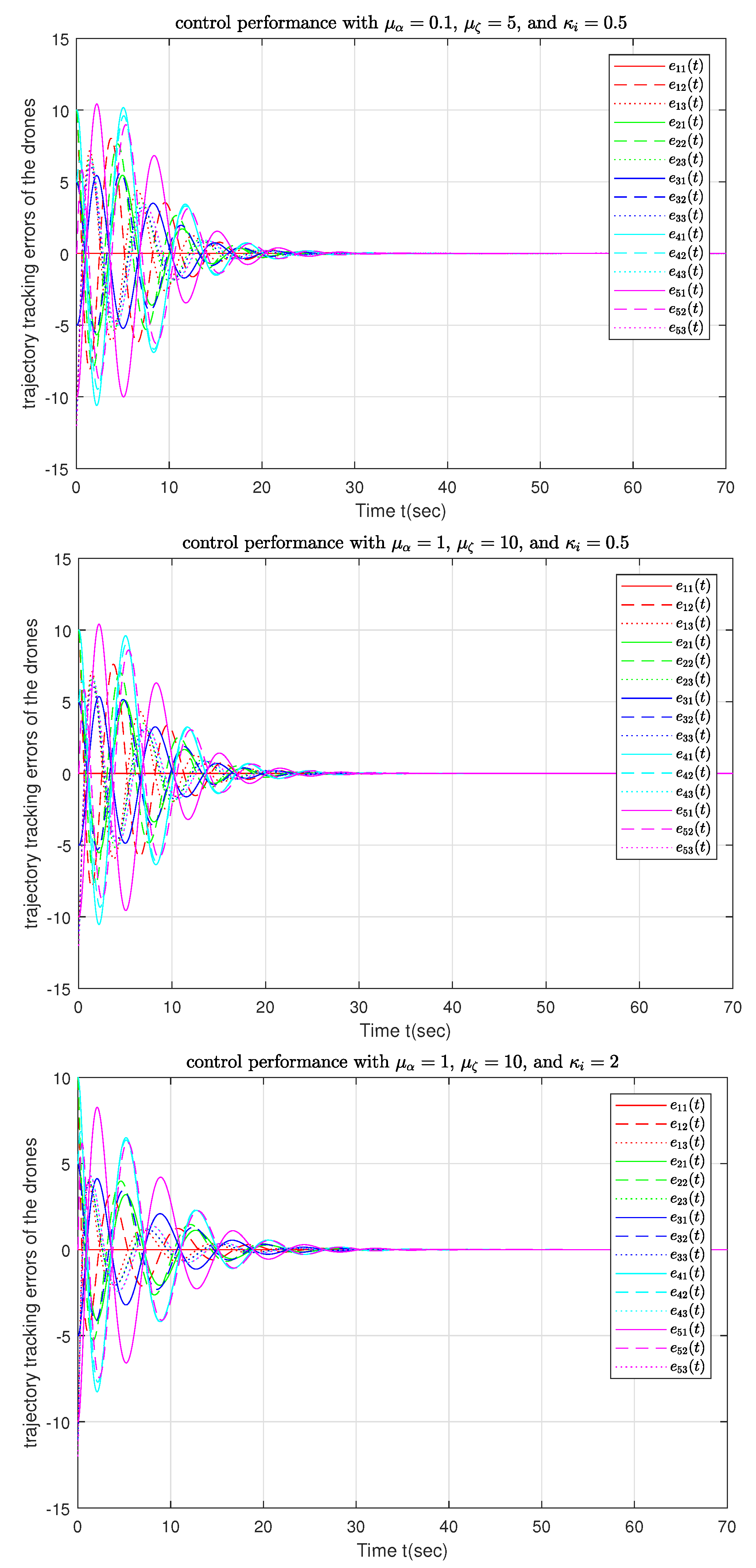
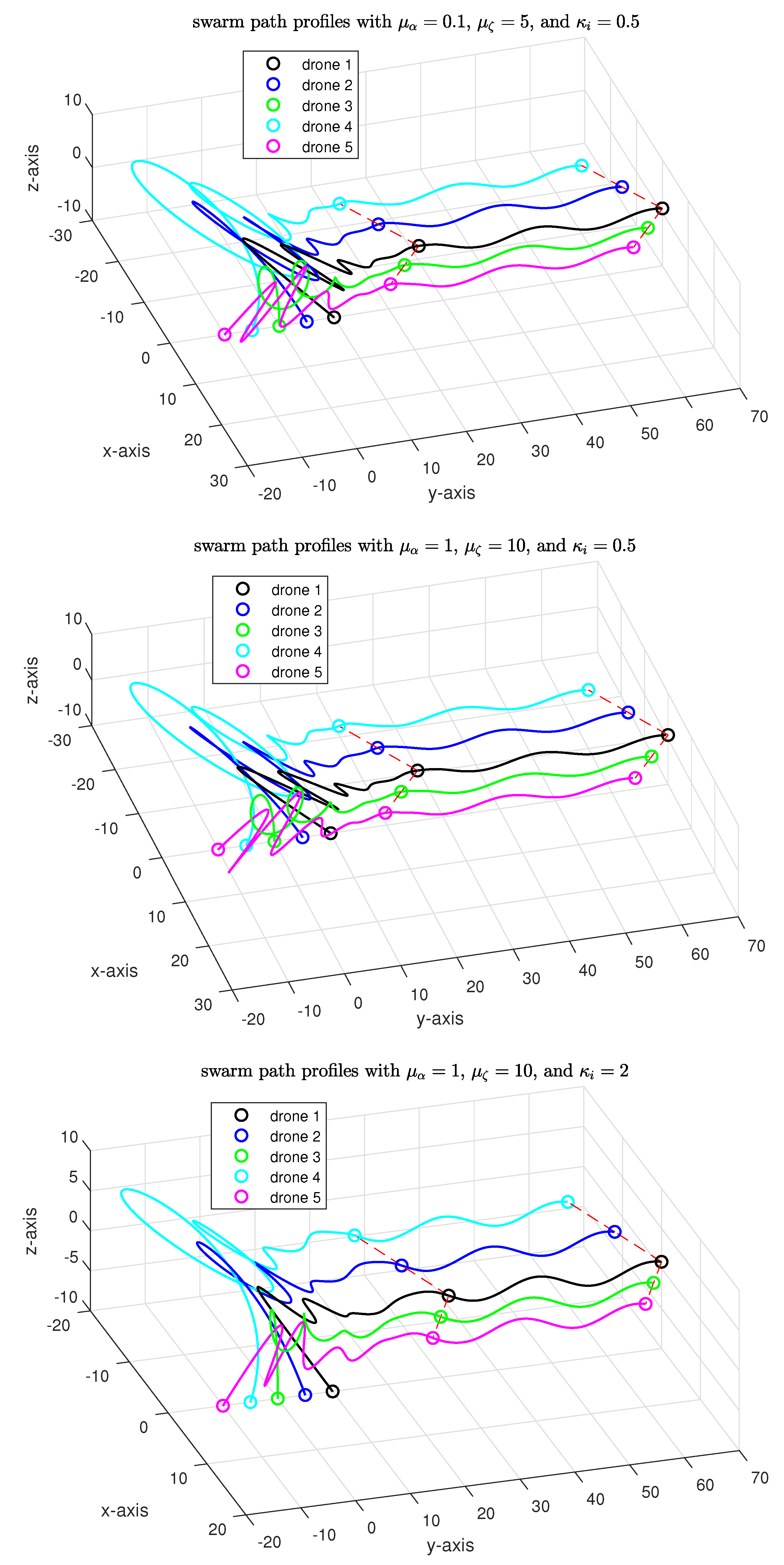
5. Numerical Simulations

In this section, a numerical simulation is given to validate the effectiveness of the proposed control scheme. Consider a swarm of $N=5$ drones. The communication graph G is shown in Figure 3. It can be directly checked that Assumption 1 is satisfied.

The nominal parts and uncertain parts of the matrices in (3) are given by

$${\mathcal{E}}_i^0=2I_3,{\Gamma }_i^0=I_3,\Delta {\mathcal{E}}_i=\Delta {\Gamma }_i=i·I_3.$$

(32)

The desired formation for drones swarm is in a wedge-shape, which is shown in Figure 4.

The local formation vectors in (4) are designed to be

$$p_{f1}=\left[\begin{array}{c}0\\ 0\\ 0\end{array}\right],p_{f2}=\left[\begin{array}{c}-5\\ -5\\ 1\end{array}\right],p_{f3}=\left[\begin{array}{c}5\\ -5\\ 1\end{array}\right],p_{f4}=\left[\begin{array}{c}-10\\ -10\\ 2\end{array}\right],p_{f5}=\left[\begin{array}{c}10\\ -10\\ 2\end{array}\right].$$

Note that $p_{f1}=\mathrm{col}(0,0,0)$ means that the trajectory of drone 1 coincides with the trajectory of the global flying path. The global flying path vector is designed to be $p_0\left(t\right)=\mathrm{col}(0,t,sin\omega t)$ with $\omega =0.3\mathrm{rad}/\mathrm{s}$. $p_0\left(t\right)$ can be generated by the linear autonomous virtual leader system (6), where the constant matrices in (6) are given by

$$S_0=\left[\begin{array}{cccc}0& 1& 0& 0\\ 0& 0& 0& 0\\ 0& 0& 0& 1\\ 0& 0& -{\omega }^2& 0\end{array}\right],W_0=\left[\begin{array}{cccc}0& 0& 0& 0\\ 1& 0& 0& 0\\ 0& 0& 1& 0\end{array}\right].$$

(33)

The initial value of the linear autonomous virtual leader system is $r_0\left(0\right)=\mathrm{col}(0,1,0,\omega )$. Besides, the minimal polynomial of $S_0$ is ${\Phi }_{S_0}^m\left(\lambda \right)={\lambda }^4+{\omega }^2{\lambda }^2$.

In the simulation example, the initial positions for the drones are given by

$$\begin{array}{cc}\hfill p_1\left(0\right)& =\left[\begin{array}{c}0\\ 10\\ -10\end{array}\right],p_2\left(0\right)=\left[\begin{array}{c}0\\ 5\\ -10\end{array}\right],p_3\left(0\right)=\left[\begin{array}{c}0\\ 0\\ -10\end{array}\right]\hfill \\ \hfill p_4\left(0\right)& =\left[\begin{array}{c}0\\ -5\\ -10\end{array}\right],p_5\left(0\right)=\left[\begin{array}{c}0\\ -10\\ -10\end{array}\right]\hfill \end{array}$$

and the initial velocities of all the drones are set to be zero.

By selecting the gains of the adaptive distributed observers and the dynamic state feedback control to be

• Gain Set 1: ${\mu }_{\alpha }=0.1$, ${\mu }_{\zeta }=5$, ${\kappa }_i=0.5$,
• Gain Set 2: ${\mu }_{\alpha }=1$, ${\mu }_{\zeta }=10$, ${\kappa }_i=0.5$,
• Gain Set 3: ${\mu }_{\alpha }=1$, ${\mu }_{\zeta }=10$, ${\kappa }_i=2$

the performance of the fully distributed robust control scheme is shown by Figure 5 and Figure 6, where Figure 5 shows the trajectory tracking errors of the drones under different control gains, and Figure 6 shows the swarm path profiles under different control gains. For all these three cases, it can be seen that the control objective has been successfully achieved. By comparing the results obtained under gain sets 1 and 2, it is found that the gains of the adaptive distributed observers ${\mu }_{\alpha },{\mu }_{\zeta }$ do not affect much the control performance. Meanwhile, by comparing the results obtained under gain sets 2 and 3, it can be observed that the average oscillation amplitudes of the tracking errors are smaller for larger dynamic state feedback control gains ${\kappa }_i$.

6. Conclusions

This paper solves the robust formation flying control problem for a swarm of drones by a fully distributed robust control scheme. By utilizing the output-based adaptive distributed observer to recover the necessary information of the virtual leader, an asymptotic internal model is conceived, which together with a certainty equivalent dynamic state feedback controller solves the robust formation flying problem for the drones’ swarm in a distributed way. In this paper, the communication network is assumed to be static and reliable. In the future, it would be interesting to further consider the case of unreliable communication networks.

References

1. Bajec, I.L.; Heppner, F.H. Organized flight in birds. Anim. Behav. 2009, 78, 777–789. [Google Scholar] [CrossRef]
2. Niwa, H.S. Self-organizing Dynamic Model of Fish Schooling. J. Theor. Biol. 1994, 171, 123–136. [Google Scholar] [CrossRef]
3. Portugal, S. Lissaman, Shollenberger and formation flight in birds. J. Exp. Biol. 2016, 219, 2778–2780. [Google Scholar] [CrossRef]
4. Desai, J.; Ostrowski, J.; Kumar, V. Modeling and control of formations of nonholonomic mobile robots. IEEE Trans. Robot. Autom. 2001, 17, 905–908. [Google Scholar] [CrossRef]
5. Shafiq, M.; Ali, Z.A.; Israr, A.; Alkhammash, E.H.; Hadjouni, M. A Multi-Colony Social Learning Approach for the Self-Organization of a Swarm of UAVs. Drones 2022, 6, 104. [Google Scholar] [CrossRef]
6. Gao, Z.; Guo, G. Fixed-Time Leader-Follower Formation Control of Autonomous Underwater Vehicles With Event-Triggered Intermittent Communications. IEEE Access 2018, 6, 27902–27911. [Google Scholar] [CrossRef]
7. Bai, H.; Wen, J.T. Cooperative Load Transport: A Formation-Control Perspective. IEEE Trans. Robot. 2010, 26, 742–750. [Google Scholar] [CrossRef]
8. Xu, C.; Zhang, K.; Jiang, Y.; Niu, S.; Yang, T.; Song, H. Communication Aware UAV Swarm Surveillance Based on Hierarchical Architecture. Drones 2021, 5, 33. [Google Scholar] [CrossRef]
9. Nigam, N.; Bieniawski, S.; Kroo, I.; Vian, J. Control of Multiple UAVs for Persistent Surveillance: Algorithm and Flight Test Results. IEEE Trans. Control Syst. Technol. 2012, 20, 1236–1251. [Google Scholar] [CrossRef]
10. Zheng, R.; Liu, Y.; Sun, D. Enclosing a target by nonholonomic mobile robots with bearing-only measurements. Automatica 2015, 53, 400–407. [Google Scholar] [CrossRef]
11. Oh, K.K.; Park, M.C.; Ahn, H.S. A survey of multi-agent formation control. Automatica 2015, 53, 424–440. [Google Scholar] [CrossRef]
12. Liu, Y.; Bucknall, R. A survey of formation control and motion planning of multiple unmanned vehicles. Robotica 2018, 36, 1019–1047. [Google Scholar] [CrossRef]
13. Kamel, M.A.; Yu, X.; Zhang, Y. Formation control and coordination of multiple unmanned ground vehicles in normal and faulty situations: A review. Annu. Rev. Control 2020, 49, 128–144. [Google Scholar] [CrossRef]
14. Balch, T.; Arkin, R. Behavior-based formation control for multirobot teams. IEEE Trans. Robot. Autom. 1998, 14, 926–939. [Google Scholar] [CrossRef]
15. Lawton, J.; Beard, R.; Young, B. A decentralized approach to formation maneuvers. IEEE Trans. Robot. Autom. 2003, 19, 933–941. [Google Scholar] [CrossRef]
16. Wang, C.; Wang, D.; Gu, M.; Huang, H.; Wang, Z.; Yuan, Y.; Zhu, X.; Wei, W.; Fan, Z. Bioinspired Environment Exploration Algorithm in Swarm Based on Levy Flight and Improved Artificial Potential Field. Drones 2022, 6, 122. [Google Scholar] [CrossRef]
17. Tanner, H.; Pappas, G.; Kumar, V. Leader-to-formation stability. IEEE Trans. Robot. Autom. 2004, 20, 443–455. [Google Scholar] [CrossRef]
18. Liang, X.; Liu, Y.H.; Wang, H.; Chen, W.; Xing, K.; Liu, T. Leader-Following Formation Tracking Control of Mobile Robots Without Direct Position Measurements. IEEE Trans. Autom. Control 2016, 61, 4131–4137. [Google Scholar] [CrossRef]
19. Dong, X.; Yu, B.; Shi, Z.; Zhong, Y. Time-Varying Formation Control for Unmanned Aerial Vehicles: Theories and Applications. IEEE Trans. Control Syst. Technol. 2015, 23, 340–348. [Google Scholar] [CrossRef]
20. Dong, X.; Hu, G. Time-varying formation control for general linear multi-agent systems with switching directed topologies. Automatica 2016, 73, 47–55. [Google Scholar] [CrossRef]
21. Dong, X.; Hu, G. Time-Varying Formation Tracking for Linear Multiagent Systems with Multiple Leaders. IEEE Trans. Autom. Control 2017, 62, 3658–3664. [Google Scholar] [CrossRef]
22. Ren, W.; Beard, R.W.; Atkins, E.M. Information consensus in multivehicle cooperative control. IEEE Control Syst. Mag. 2007, 27, 71–82. [Google Scholar] [CrossRef]
23. Ren, W.; Beard, R. Consensus seeking in multiagent systems under dynamically changing interaction topologies. IEEE Trans. Autom. Control 2005, 50, 655–661. [Google Scholar] [CrossRef]
24. Olfati-Saber, R.; Fax, J.A.; Murray, R.M. Consensus and Cooperation in Networked Multi-Agent Systems. Proc. IEEE 2007, 95, 215–233. [Google Scholar] [CrossRef]
25. Olfati-Saber, R.; Murray, R. Consensus problems in networks of agents with switching topology and time-delays. IEEE Trans. Autom. Control 2004, 49, 1520–1533. [Google Scholar] [CrossRef]
26. Cai, H.; Su, Y.; Huang, J. Cooperative Control of Multi-Agent Systems: Distributed-Observer and Distributed-Internal-Model Approaches; Springer: Cham, Switzerland, 2022. [Google Scholar]
27. Wang, X. Distributed formation output regulation of switching heterogeneous multi-agent systems. Int. J. Syst. Sci. 2013, 44, 2004–2014. [Google Scholar] [CrossRef]
28. Hua, Y.; Dong, X.; Hu, G.; Li, Q.; Ren, Z. Distributed Time-Varying Output Formation Tracking for Heterogeneous Linear Multiagent Systems With a Nonautonomous Leader of Unknown Input. IEEE Trans. Autom. Control 2019, 64, 4292–4299. [Google Scholar] [CrossRef]
29. Hua, Y.; Dong, X.; Li, Q.; Ren, Z. Distributed adaptive formation tracking for heterogeneous multiagent systems with multiple nonidentical leaders and without well-informed follower. Int. J. Robust Nonlinear Control 2020, 30, 2131–2151. [Google Scholar] [CrossRef]
30. Song, W.; Feng, J.; Zhang, H.; Wang, W. Dynamic Event-Triggered Formation Control for Heterogeneous Multiagent Systems With Nonautonomous Leader Agent. IEEE Trans. Neural Netw. Learn. Syst. 2022, 1–15. [Google Scholar] [CrossRef] [PubMed]
31. Li, W.; Chen, Z.; Liu, Z. Formation control for nonlinear multi-agent systems by robust output regulation. Neurocomputing 2014, 140, 114–120. [Google Scholar] [CrossRef]
32. Huang, X.; Dong, J. Reliable Leader-to-Follower Formation Control of Multiagent Systems Under Communication Quantization and Attacks. IEEE Trans. Syst. Man Cybern. Syst. 2020, 50, 89–99. [Google Scholar] [CrossRef]
33. Li, W.; Zhang, H.; Ming, Z.; Wang, Y. Fully Distributed Event-Triggered Bipartite Formation Tracking Control for Heterogeneous Multi-Agent Systems on Signed Digraph. IEEE Trans. Circuits Syst. II Express Briefs 2022, 69, 2181–2185. [Google Scholar] [CrossRef]
34. Zhang, H.; Li, W.; Zhang, J.; Wang, Y.; Sun, J. Fully Distributed Dynamic Event-Triggered Bipartite Formation Tracking for Multiagent Systems With Multiple Nonautonomous Leaders. IEEE Trans. Neural Netw. Learn. Syst. 2022, 1–14. [Google Scholar] [CrossRef] [PubMed]
35. Jiang, D.; Wen, G.; Peng, Z.; Huang, T.; Rahmani, A. Fully Distributed Dual-Terminal Event-Triggered Bipartite Output Containment Control of Heterogeneous Systems Under Actuator Faults. IEEE Trans. Syst. Man Cybern. Syst. 2022, 52, 5518–5531. [Google Scholar] [CrossRef]
36. Jiang, D.; Wen, G.; Peng, Z.; Wang, J.L.; Huang, T. Fully Distributed Pull-Based Event-Triggered Bipartite Fixed-Time Output Control of Heterogeneous Systems with an Active Leader. IEEE Trans. Cybern. 2022, 1–12. [Google Scholar] [CrossRef]
37. Cai, H.; Huang, J. Output based adaptive distributed output observer for leader–follower multiagent systems. Automatica 2021, 125, 109413. [Google Scholar] [CrossRef]
38. Cai, H.; Lewis, F.L.; Hu, G.; Huang, J. The adaptive distributed observer approach to the cooperative output regulation of linear multi-agent systems. Automatica 2017, 75, 299–305. [Google Scholar] [CrossRef]
39. Yan, J.; Yu, Y.; Wang, X. Distance-Based Formation Control for Fixed-Wing UAVs with Input Constraints: A Low Gain Method. Drones 2022, 6, 159. [Google Scholar] [CrossRef]
40. Nguyen, N.P.; Park, D.; Ngoc, D.N.; Xuan-Mung, N.; Huynh, T.T.; Nguyen, T.N.; Hong, S.K. Quadrotor Formation Control via Terminal Sliding Mode Approach: Theory and Experiment Results. Drones 2022, 6, 172. [Google Scholar] [CrossRef]
41. Huang, J. Nonlinear Output Regulation: Theory and Applications; SIAM: Philadelphia, PA, USA, 2004. [Google Scholar]
Figure 1. The structure of the fully distributed robust control scheme for an individual drone.
Drones 06 00266 g001
Figure 2. The external and internal signal transmission for the fully distributed robust control scheme. Here, VL, ADO, AIM, and DFC are short for virtual leader, adaptive distributed observer, asymptotic internal model, and dynamic feedback control, respectively.
Drones 06 00266 g002
Figure 3. Communication graph G. Here, node 0 represents the virtual leader, and node i, i = 1 , , 5 , represents the ith drone.
Drones 06 00266 g003
Figure 4. Desired wedge-shape formation for the drones swarm.
Drones 06 00266 g004
Figure 5. Trajectory tracking errors of the drones under different control gains.
Drones 06 00266 g005
Figure 6. Swarm path profiles under different control gains.
Drones 06 00266 g006
Publisher’s Note: MDPI stays neutral with regard to jurisdictional claims in published maps and institutional affiliations.