UAV Path Planning Based on Multi-Stage Constraint Optimization

Abstract

Evolutionary Algorithms (EAs) based Unmanned Aerial Vehicle (UAV) path planners have been extensively studied for their effectiveness and high concurrency. However, when there are many obstacles, the path can easily violate constraints during the evolutionary process. Even if a single waypoint causes a few constraint violations, the algorithm will discard these solutions. In this paper, path planning is constructed as a multi-objective optimization problem with constraints in a three-dimensional terrain scenario. To solve this problem in an effective way, this paper proposes an evolutionary algorithm based on multi-level constraint processing (ANSGA-III-PPS) to plan the shortest collision-free flight path of a gliding UAV. The proposed algorithm uses an adaptive constraint processing mechanism to improve different path constraints in a three-dimensional environment and uses an improved adaptive non-dominated sorting genetic algorithm (third edition—ANSGA-III) to enhance the algorithm’s path planning ability in a complex environment. The experimental results show that compared with the other four algorithms, ANSGA-III-PPS achieves the best solution performance. This not only validates the effect of the proposed algorithm, but also enriches and improves the research results of UAV path planning.

1. Introduction

In past decades, with the increasing maturity of UAV technology, the application scenarios of UAVs have diversified, including logistics, communications, rescue, military, and other fields. Autonomous path planning of UAVs has become a research hotspot [1,2,3,4]. The main goal of this problem is to find the optimal flight path between the source and destination without colliding with any no-fly zone or obstacle in the environment [5].

A significant difference between UAV path planning and general path planning is that the UAV path search space is a three-dimensional space, which makes the search range larger and the solution more difficult. In research, the UAV path planning problem has attracted a large number of optimization applications. Recently reported by Qu et al. [6], proposed a multi-strategy combination evolutionary algorithm. They analyzed the characteristics of each main link in the UAV path planning process and proposed optimization strategies such as length operation and smooth operation, which improved the quality of the solution. The author of [7] proposed the rotation transformation of the Cartesian coordinate system to enhance its local modification ability and divide the entire search space into multiple subspaces to reduce the scope of the search space. At the same time, they designed a path planner estimation method based on distributed algorithm (EDA). The author of [8] studied the obstacle processing strategy in the UAV path planning process, emphasizing the processing of the dimension of height. A multi-objective integer programming model of UAV flight path was proposed by establishing a mathematical model through three-dimensional grid cells. The author of [9] proposed an algorithm based on the clustering idea, which divides the region of waypoints of different individuals through clustering and obtains the approximate optimal waypoint of UAV so as to guide the generation of offspring. In [10,11], the authors studied the characteristics of the evolutionary algorithm (EA), analyzed the main problems in evolutionary algorithm path planning, and established an evaluation system for a single path point.

The UAV path planning problem is a typical constrained optimization problem. However, there has been relatively little research on constraint strategies in UAV path planning. In the problem of UAV flight path planning, there are two situations that violate constraints. One is caused by a single waypoint constraint violation, and the other is caused by a path segment. Therefore, when the evolutionary algorithm is used to solve the path planning problem, even if the fitness of a single waypoint is good and the constraint conditions are met, the path segment composed of these waypoints may be an infeasible solution. Reference [12] proposed an improved differential evolution algorithm (MOEAD) to realize UAV path planning, where the feasible solution superiority mechanism similar to that in [13] is adopted to solve the constraint problem of UAV. Reference [14], the author proposed an algorithm combining simulated annealing and genetic algorithm(GA) to carry out path planning. In reference [15], the author proposes a hybrid path planning (HPP) algorithm to efficiently collect data by ensuring the shortest collision-free path for UAVs in emergency situations. The HPP algorithm first uses the probabilistic roadmap method to get the shortest collision-free route and then uses the improved artificial bee colony algorithm to dynamically optimize the collision constraints.

When planning a route for a UAV, many important factors need to be considered, such as the dynamics of the drone, the environment of the mission space, the safety and cost of the route. These factors either exist as an objective function that needs to be maximized/minimized, or as constraints that the path must comply with. In the past, researchers are committed to establishing evaluation criteria based on single-path optimization goals or constraint goals and emphasize the optimization of a single path in generation strategies. However, in UAV path planning, neither the emphasis on the optimization of the objective functions nor the optimization of the constraints can guarantee that the whole path segment, composed of single favorable path points, will be advantageous. In this paper, we present a multi-stage UAV path planning algorithm to solve the above problems. We divide the path planning process into two stages. In the first stage, local optimal paths with a few constraints are generated, and then in the second stage, these local optimal paths are optimized to get a global optimal path that satisfies all constraints. Aiming at different stages of the algorithm, an improved targeted mutation strategy enhances the algorithm’s ability to jump out of constrained regions and search in narrow feasible regions.

The rest of this article is organized as follows. In Section 2, the UAV path planning model and the details of the proposed ANSGA-III-PPS are described. Then, the proposed algorithm’s performance is evaluated via computer simulation and compared with the other four algorithms in Section 3. In Section 4, the experimental results and the differences between the proposed algorithm and the comparison algorithm are analyzed. Finally, Section 5 summarizes the article.

2. Multi-Stage Constrained Optimization Algorithm for UAV Path Planning

This section provides a multi-stage constrained optimization method for UAV path planning. In the following subsections, we first formally state the problem of interest and then introduce our method in detail.

2.1. Problem Statement

In recent years, UAVs have been widely applied in various disaster relief applications, such as detecting disaster situations, placing supplies, assisting in rescue operations, and so on. When performing rescue missions, these UAVs should be deployed to the disaster site as soon as possible. This means that the shorter the flight path of the UAVs, the better. On the other hand, when performing reconnaissance missions, these UAVs should keep flying as low as possible to get more accurate information. However, there are many challenges in the mission environment, such as mountains and no-fly zones. They pose an enormous threat to the safety and maneuverability of UAVs. Therefore, in the lock of decision-makers’ preference information, the goal of path planning is to minimize the flight distance and flight height while satisfying the UAV’s dynamic constraints and mission environment constraints. It can be considered that this problem is a constrained multi-objective optimization problem, which can be mathematically defined as

$$\begin{gathered} \mathrm{Minimize} F\left(x_{*}\right)=\left(f_1\left(x\right),\dots ,f_m\left(x\right)\right) \\ {g}_i\left(x\right)\le 0,i=1,\dots ,\mathrm{p} \\ {h}_j\left(x\right) =0,j=1,\dots ,\mathrm{q} \\ x\in \mathsf{\Omega }. \end{gathered}$$

(1)

In Formula (1), $x=\left(x_1,\dots ,x_{\mathrm{D}}\right)$ is the solution consisting of D decision variables, $\mathsf{\Omega }$ is the decision space, $x_{*}$ is the pareto optimal set, $F=\left(f_1,\dots ,f_m\right)$ is the objective function and M is the number of objectives. $g_i\left(x\right)$ and $h_j\left(x\right)$ are inequality and equality constraints, p and q represent the number of inequalities and equality constraints, respectively.

In the UAV path planning problem, obstacles can only be dealt with by going around or flying over them, while gliding drones usually require a certain distance and time to change direction, which makes it more difficult to solve the path optimization problem of gliding drones. Therefore, this paper proposes a multi-objective optimization algorithm to solve the path planning problem of gliding UAVs in a multi-obstacle environment. Specifically, the resulting flight trajectory must satisfy the following constraints: (1) The flight path is safe and feasible, one is to prohibit drones from colliding with terrain obstacles. Second, it is not allowed to enter the no-fly zone. Finally, the drone maintains a minimum flight distance from the ground. (2) The dynamic index of gliding drone must be met. According to the characteristics of the gliding UAV, the dynamic indicators include the maximum turning angle, the maximum climb angle and the shortest commutation distance.

Under the premise of satisfying the above constraints, the path must be optimized as much as possible. The objective of optimization is to make the path shorter and the height fluctuation smaller. We first introduce the basic terrain features of the mission space environment and the representation method of the UAV flight path, to clearly describe the mathematical model established for the proposed problem.

2.1.1. Representation of Terrain and Route

The terrain environment is constructed using the inertial reference system OXYZ, which consists of two parts: the mountain topography and the no-fly zone. The no-fly zone can be represented by a cylinder, and the mountain topography is generated by the equivalent digital map proposed in [16], which can more truly reflect the threat range of the terrain. First, the original digital terrain is generated by Formula (2).

$$h_1\left(x,y\right)=sin(y÷180+1.5\times \pi )+0.1\times sin(x÷16)+0.9\times \mathit{cos}(0.3\times median)+0.01\times \mathit{sin}(0.01\times median)+0.3\times \mathit{cos}(y÷36).$$

(2)

$h_1\left(x,y\right)$ represents the height of the terrain corresponding to the point $\left(x,y\right)$, where the $median=\sqrt{({(x÷16)}^2+\left(y÷36{)}^2\right)÷5}$.

Then, in order to reflect the terrain slope of the mountain, the mountain topography is generated by Formula (3).

$$h_2\left(x,y\right)={{\displaystyle \sum }}_{k=1}^{K}h\left(K\right)\times \mathit{exp}(-{(x-o_1\left(K\right))}^2÷L_1\left(K\right)-\left(y-o_2\left(K\right){)}^2÷L_2\left(K\right)\right).$$

(3)

In Formula (3), $h_2\left(x,y\right)$ represents the height of the peak corresponding to the point $\left(x,y\right)$, $K$ represents the number of mountain peaks, $h\left(K\right)$ is the highest height of the Kth peak, ($o_1\left(K\right)$, $o_2\left(K\right)$) is the horizontal coordinate of the center of the Kth peak, and $L_1\left(K\right)$ and $L_2\left(K\right)$ control the contour of the Kth peak.

Finally, the terrain threat equivalent map is fused with the original digital terrain to generate an equivalent digital map by Formula (4).

$$\mathrm{Map}\left(x,y\right)=\mathit{max}(h_1\left(x,y\right),h_2\left(x,y\right)).$$

(4)

In this paper, a coding method similar to the traveling salesman problem is used to represent the flight path. In a population of size $N$, the track of each individual is represented by a sequence of waypoints, and the number of waypoints is set as $N_w$.

$$X_i=(x_s,y_s,z_s,\dots ,x_j,y_j,z_j,\dots ,x_e,y_e,z_e),x_j\in \left[0,X_{max}\right],y_j\in \left[0,Y_{max}\right],z_j\in \left[0,Z_{max}\right],i=1\dots N,j=1\dots N_w$$

where $X_i$ is the path of the ith individual in the population; $s$ and $e$ represent the starting point and end point of the track, respectively; $j$ is the number of the waypoint in a single flight path; and $\left(x_j,y_j,z_j\right)$ is the coordinate value of the $j$th waypoint.

It should be noted that the mission environment of the UAV path planning problem is a continuous space. Therefore, in the solution process, $N_m$ sampling points are uniformly selected on the linear trajectory of the two waypoints to detect the position information. As shown in Figure 1, when the position information of $N_m$ points does not collide with obstacles, the feasibility of the trajectory can be ensured [11].

2.1.2. Objective Functions and Performance Constraints

According to the problem description in Section 2.1, we constructed 2 objective functions and 5 constraint functions, and the design of each function is as follows:

• Objective Functions
  • Minimum length

    $$min{f}_1=\frac{{{\displaystyle \sum }}_{j=2}^{N_w}\sqrt{{(x_j-x_{j-1})}^2+{(y_j-y_{j-1})}^2+{(z_j-z_{j-1})}^2}}{\sqrt{{(x_e-x_s)}^2+{(y_e-y_s)}^2+{(z_e-z_s)}^2}}.$$

    (5)

The path of each individual in the population is represented by a sequence of waypoints ($N_w$ indicates the number of path points), so the objective function, $f_1$ (distance function), is the ratio of the Euclidean distance of all waypoints to the straight-line distance from the start point to the end point. The smaller the ratio, the closer it is to the shortest distance.

• 2.

  Minimum flying altitude

  $$\begin{gathered} min{f}_2=\frac{{{\displaystyle \sum }}_{j=2}^{N_w}{{\displaystyle \sum }}_{m=1}^{N_m}\mathit{max}(p{z}_{j,m}-h_{j,m},0)}{\left(N_w-1\right)\times N_m} \\ p{x}_{j,m}=x_{j-1}+\frac{m}{N_m}\times \left(x_j-x_{j-1}\right),m=2\dots N_m-1 \\ p{y}_{j,m}=y_{j-1}+\frac{m}{N_m}\times \left(y_j-y_{j-1}\right),m=2\dots N_m-1 \\ p{z}_{j,m}=z_{j-1}+\frac{m}{N_m}\times \left(z_j-z_{j-1}\right),m=2\dots N_m-1 \\ {h}_{j,m}=map\left(p{x}_{j,m},p{y}_{j,m}\right). \end{gathered}$$

  (6)

The objective function $f_2$ is an altitude function, and $p{x}_{j,m}$ is the X-axis value of the mth sampling point on the segment between (j−1)th and jth waypoint. Similarly, we can calculate the Y-axis and Z-axis values of each sampling point. In particular, $\left(p{x}_{j,1},p{y}_{j,1},p{z}_{j,1}\right)$ and $\left(p{x}_{j,N_m},p{y}_{j,N_m},p{z}_{j,N_m}\right)$ are the values of (j−1)th and jth waypoint, respectively. $h_{j,m}$ is the map height of the mth sampling point. The smaller the ratio of the objective function $f_2,$ the lower the flight altitude of the entire flight path.

• Constraint Functions
  • Angle constraint

$$\begin{gathered} g_1={\displaystyle \sum }_{j=2}^{N_w-1}{c}_j^1 \\ {c}_j^1=\{\begin{array}{c}0\hspace{0.17em}\hspace{0.17em}\hspace{0.17em}\hspace{0.17em}\hspace{0.17em}\hspace{0.17em}\hspace{0.17em}\hspace{0.17em}\hspace{0.17em}\hspace{0.17em}\hspace{0.17em}\hspace{0.17em} , {\theta }_j<{\theta }_{max}\\ \frac{\mathit{cos}({\theta }_{max})-\mathit{cos}({\theta }_j)}{\mathit{cos}({\theta }_{max})-\mathit{cos}({180}^{\circ })}, otherwise\end{array} \\ {\theta }_j=\mathit{arccos}\frac{\left(x_j-x_{j-1},y_j-y_{j-1}\right)\cdot \left(x_{j+1}-x_j,y_{j+1}-y_j\right)}{||\left(x_j-x_{j-1},y_j-y_{j-1}\right)||\times ||\left(x_{j+1}-x_j,y_{j+1}-y_j\right)||} . \end{gathered}$$

(7)

where ${\theta }_{max}$ is the predetermined upper limit of the turning angle, ${\theta }_j$ is the turning angle at the jth waypoint, and the $||x||$ means the norm of vector $x$.

• 2.

  Climbing angle constraint

$$\begin{gathered} g_2={\displaystyle \sum }_{j=2}^{N_w}{c}_j^2 \\ {c}_j^2=\{\begin{array}{c}0\hspace{0.17em}\hspace{0.17em}\hspace{0.17em}\hspace{0.17em}\hspace{0.17em}\hspace{0.17em}\hspace{0.17em}\hspace{0.17em}, {\alpha }_j<{\alpha }_{max}\\ 1-\frac{\mathit{tan}\left({\alpha }_{max}\right)}{\mathit{tan}({\alpha }_j)} , otherwise\end{array} \\ {\alpha }_j=\mathit{arccos}\frac{\left|z_j-z_{j-1}\right|}{||\left(x_j-x_{j-1},y_j-y_{j-1}\right)||}. \end{gathered}$$

(8)

Here, ${\alpha }_j$ is the climb angle of the jth waypoint; when ${\alpha }_j$ is greater than the predetermined maximum climb angle ${\alpha }_{max}$, the constraint is recorded as constraint $c_j^2$.

• 3.

  Obstacle avoidance constraints

$$\begin{gathered} g_3={\displaystyle \sum }_{j=2}^{N_w}{c}_j^3 \\ {c}_j^3=\frac{{{\displaystyle \sum }}_{m=1}^{N_m}{c}_{j,m}^3}{cn\left(j\right)} \\ {c}_{j,m}^3=\{\begin{array}{l}0\hspace{0.17em}\hspace{0.17em}\hspace{0.17em}\hspace{0.17em}\hspace{0.17em}\hspace{0.17em}\hspace{0.17em}, p{z}_{j,m}-h_{j,m}<h_{min}\\ 1-\frac{p{z}_{j,m}}{h_{j,m}+h_{min}} , otherwise\end{array}. \end{gathered}$$

(9)

The calculation of $p{z}_{j,m}$ and $h_{j,m}$ is the same as shown in Formula (6); when the vertical distance between $p{z}_{j,m}$ and the terrain height $h_{j,m}$, is less than the safe flight height $h_{min}$, the mth sampling point violates the obstacle avoidance constraint $c_{j,m}^3$. Where $cn\left(j\right)$ is the number of sampling points that violate constraint $c_{j,m}^3$.

• 4.

  Minimum flight distance constraint

$$\begin{gathered} g_4={\displaystyle \sum }_{j=2}^{N_w}{c}_j^4 \\ {c}_j^4=\{\begin{array}{l}0\hspace{0.17em}\hspace{0.17em}\hspace{0.17em}\hspace{0.17em}\hspace{0.17em}\hspace{0.17em} , d_j>L_{min}\\ 1-\frac{d_j}{L_{min}} , otherwise\end{array} \\ {d}_j=\sqrt{{(x_j-x_{j-1})}^2+{(y_j-y_{j-1})}^2+{(z_j-z_{j-1})}^2}. \end{gathered}$$

(10)

The gliding drone needs the minimum distance $L_{min}$ to adjust height or angle. When the distance between two adjacent waypoints is less than the shortest flight distance, the violation value is denoted as $c_j^4$.

• 5.

  No-fly zone restrictions

$$\begin{gathered} g_5={\displaystyle \sum }_{j=2}^{N_w-1}{c}_j^5 \\ {c}_j^5=\frac{{{\displaystyle \sum }}_{m=1}^{N_m}{c}_{j,m}^5}{cn\left(j\right)} \\ {c}_{j,m}^5=\{\begin{array}{c}0\hspace{0.17em}\hspace{0.17em}\hspace{0.17em}\hspace{0.17em} , p{t}_{j,m,i}<r_i,i=1\dots k\\ \frac{p{t}_{j,m,i}}{r_i} ; otherwise\end{array} \\ p{t}_{j,m,i}=\sqrt{{(p{x}_{j,m}-t{x}_i)}^2+{(p{y}_{j,m}-t{y}_i)}^2}. \end{gathered}$$

(11)

$\left(t{x}_k,t{y}_k,h_{max},r_k\right)$ contains all the information of the no-fly zone, where $\left(t{x}_k,t{y}_k\right)$ represents the bottom center coordinates of the kth no-fly zone, $h_{max}$ represents the maximum altitude of the mission environment (the no-fly zone cannot be overflown), and $r_k$ is the detection radius of the kth no-fly zone. In Formula (11), $p{t}_{j,m,i}$ is the Euclidean distance between the sampling point $\left(p{x}_{j,m},p{y}_{j,m}\right)$ and the no-fly zone coordinate point $\left(t{x}_k,t{y}_k\right)$.

• Overall constraint violation

  $$CV\left(x\right)={\displaystyle \sum }_{i=1}^G{g}_i$$

  (12)

To deal with a set of constraints in CMOPs, the overall constraint violation is a widely used approach, which summarizes the violations into a single scalar. The overall constraint violation calculation method is given in Formula (12). Where $CV\left(x\right)$ is the overall constraint violation of individual $x$, $g_i$ is the violation value of the ith inequality constraint, and $G$ is the total number of all inequality constraints.

2.2. The Proposed Algorithm

Evolutionary algorithms (EAs) follow a similar framework. First, initialize the population. When the termination condition is not met, the generation strategy is used to generate new individuals according to the current population information in each iteration. Second, the constraint processing strategy is used to combine the constraint violation value and individual fitness to form individual advantage. Finally, the dominant individuals are selected through the environmental selection mechanism to form the next generation population. The generation operation and retention operation are repeated until the termination condition is satisfied, and the last generation population is output as the optimal solution. Therefore, identifying and producing excellent individuals in each generation is a decisive factor in obtaining the optimal solution.

In this paper, the multi-stage constraint processing framework of push-pull search (PPS) and adaptive reference point selection mechanism are used to enhance the ability to identify dominant individuals. On the other hand, a generation strategy combining crossover mechanisms with an improved targeted mutation method to enhances the ability to produce offspring within a narrow feasible region. The pseudocode of ANSGA-III-PPS is presented in Algorithm 1. To introduce the proposed algorithm in detail, each key component is described one by one in this section.

Algorithm 1 ANSGA-III-PPS
Input: $N$: the number of population; $T_{max}$: the maximum generation; $T_c$: maximum relaxation control generation; $N_w$: the max number of track points; $P_l$: the local mutation rate;
Output: $P_{Tmax}$: a set of feasible non-dominated solutions;
1	Initialization:
2	Set the parameters;
3	Initialize the population $P=\left(X_1 , \dots , X_N \right), X = \left(w_1 , w_2 , \dots , w_{N_w}\right), w_i = \left(x_i , y_i , z_i \right)$;
4	$z^s$ $\leftarrow$ Initialize reference point;
5	$l_{distance}$ $\leftarrow$ The distance between two reference points;
6	Evaluation (p) according to the objective function and constraint function;
7	$q_3$, $q_5$ $\leftarrow$ Create two two-dimensional arrays;
8	$PushStage=True$;
9	whileT$\le$ $T_{max}$do
10	$z\left(T\right)=Min\left(f\left(X\right)\right);$ // update ideal point at kth generation;
11	$n\left(T\right)=Max\left(f\left(X\right)\right)$; // update nadir point at kth generation;
12	for$X$ to $P$ do
13	$CV\left(X\right)$ $\leftarrow$ Calculate the total value of constraint violations according to Equation (12);
14	end
15	$rf\left(P_T\right)$ $\leftarrow$ Calculate the proportion of feasible solutions in population $P_T$;
16	$\epsilon \left(k\right),PushStage= Update constraint threshold\left(P_T,CV,rf\left(P_T\right),PushStage,z,n,T_c,T\right)$;
17	$p= Offspring generation \left(P_T, P_l, PushStage\right)$;
18	Evaluation ($p$) according to the objective function and constraint function;
19	$q_3$, $q_5$ $\leftarrow$ Update array members;
20	$R_T =\left[P_T ; p\right]$;
21	$Z^a$ $\leftarrow$ update the desired points;
22	$P_{T+1} = EnvironmentalSelection\left(R_T ,\epsilon \left(k\right), PushStage, Z^s , Z^a\right)$;
23	$Z^s = Updatepoints\left(P_{T+1}, Z^s , l_{distance}\right)$;
24	end

2.2.1. Multi-Stage Constraint Processing Strategy

The original PPS framework divides the solution process into two stages, namely the push search stage and the pull search stage [17]. In the push search stage, the population only retains those individuals with superior fitness, and the constrained optimization problem is transformed into an unconstrained problem. In the pull search stage, a relaxation constraint mechanism similar to progressive barrier (PB) approach is used to balance the relationship between optimization goals and constraints [18]. However, there are two differences involving the PB method. First, in terms of the initial setting of the relaxation constraint, the PPS framework replaces the fixed threshold setting in PB with an adaptive method. At the end of the push search stage, the largest overall constraint violation $CV\left(x\right)$ among all individuals who violated the constraints in the population is selected as the initial relaxation constraint. Second, the PPS framework can be applied to any evolutionary algorithm almost without any changes.

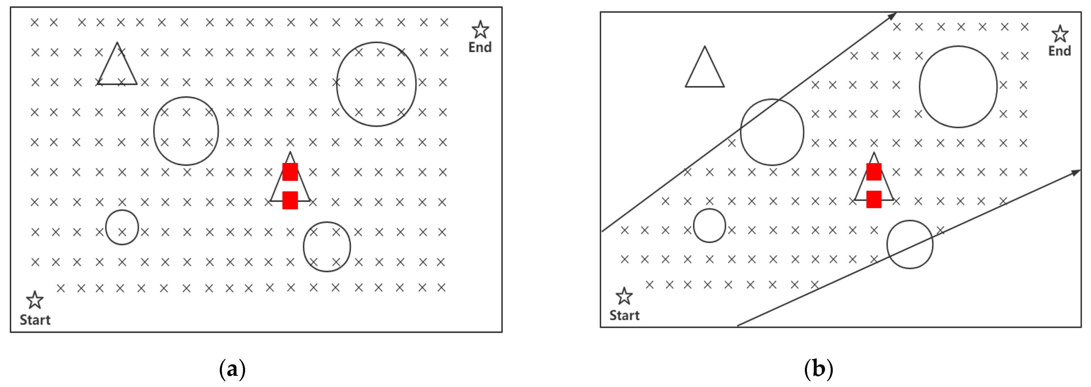
Since the obstacles in the no-fly zone can only be evaded via bypassing, this has caused the no-fly zone constraints to seriously affect the path planning effect of the gliding UAV. Therefore, this paper does not adopt the unconstrained optimization idea in the original PPS framework in the push search stage, but comprehensively considers the individual’s fitness and no-fly zone constraints to select the individual.

The constraint processing method of the push search stage used in this article is shown in Figure 2, where the circle is the no-fly zone, the triangle is the terrain obstacle, and the black cross is the path point position. At the end of the push search stage, the waypoints that violate the no-fly zone restrictions are eliminated, but the waypoints (red squares) that violate the terrain restrictions still exist. Since the influence of other constraints on the flight path is not considered, the search space will be reduced to the local optimal area.

The core of the PPS framework comprises two parts: the strategy of switching search behavior and the updating method of relaxation constraint.

• Switch search behavior strategy

The main idea of switching the search behavior strategy is to calculate the max rate of change between the ideal and nadir points during the last $l$ generations.

$$r_k\equiv \mathit{max}\{z_k,n_k\}\le \delta .$$

(13)

In Formula (13), $r_k$ represents the max rate of change, and $\delta$ is the parameter of the maximum rate of change, which is a minimum value defined by the user.

$$\begin{gathered} z_k=\underset{i=1,\dots ,m}{\mathit{max}}\frac{\left|z_i^k-z_i^{k-l}\right|}{\mathit{max}\{\left|z_i^{k-1}\right|,\mathsf{\Delta } \}},z_i^k={\mathit{min}}_{j=1,\dots ,N}{f}_i\left(x^j\right) \\ {n}_k=\underset{i=1,\dots ,m}{\mathit{max}}\frac{\left|n_i^k-n_i^{k-l}\right|}{\mathit{max}\{\left|n_i^{k-1}\right|,\mathsf{\Delta }\}},n_i^k={\mathit{max}}_{j=1,\dots ,N}{f}_i\left(x^j\right). \end{gathered}$$

(14)

In Formula (14), the calculation method of change rate is given. where $z^k=\left(z_1^k,\dots ,z_m^k\right)$, $n^k=\left(n_1^k,\dots ,n_m^k\right)$ are the ideal and nadir points in the kth generation, $N$ is population size, and the ideal and nadir points in the ($k-l$)th generation are denoted as $z_i^{k-l}$ and $n_i^{k-l}$. $\mathsf{\Delta }$ is a very small positive number used to avoid dividing by zero. In each generation after the $l$ generation, $r_k$ is update according to Formula (14). If $r_k$ is less than or equal to the parameter $\delta$, the search behavior is switched to the pull search.

• Update method of relaxation constraint

$$\epsilon \left(T\right)=\{\begin{array}{c}\left(1-\tau \right)\epsilon \left(T-1\right),r{f}_T<\alpha \\ \epsilon \left(0\right){(1-\frac{T}{T_c})}^{cp} , \mathrm{r}{f}_T\ge \alpha . \end{array}$$

(15)

The update method of the relaxation constraint $\epsilon \left(T\right)$ is listed in Formula (15), $r{f}_T$ represents the ratio of feasible and infeasible solutions in the Tth generation, and $\alpha$ is to control the searching preference between the feasible and infeasible regions ($\alpha \in \left[0,1\right]$). Different from other relaxation constraint mechanism design, two control parameters $\tau$ and $cp$ are introduced to control the speed of reducing the relaxation of constraints for different feasible solution ratios in Formula (15), which can help to find feasible solutions more quickly and efficiently. $T_c$ is the preset maximum relaxation generation, which is used to control the time when the relaxation constraint is reduced to zero.

In the push search stage, the relaxation constraint $\epsilon \left(T\right)$ is set to 0, and only when the individual’s no-fly zone constraint is greater than $\epsilon \left(T\right)$, the individual will be identified as an infeasible solution. However, in the pull search stage, Formula (15) is used to update the relaxation constraint $\epsilon \left(T\right)$, and given a solution $x$, if $CV\left(x\right)\le \epsilon \left(T\right)$, $x$ is feasible. For all infeasible solutions, additional operations are performed in the environmental selection mechanism to determine whether they can enter the next generation.

The pseudocode of the switch search behavior strategy and the update method of relaxation constraint is introduced in Algorithm 2.

Algorithm 2 Update constraint threshold

Input: $P_T$: Population of the current generation; $CV$: The total value of constraint violations of the Current iteration; $rf\left(P_T\right)$: The proportion of feasible solutions in population $P_T$; $PushStage$: Phase transition flag; $z$: Minimum fitness set for each generation; $n$: Maximum fitness set for each generation; $T_C$: The maximum relaxation iteration; $T$: Current iteration number;

Output: $\epsilon \left(k\right)$: Constraint threshold for the Tth generation; $PushStage$: Phase transition flag;

1 Initialization:

2      Set the parameters;

3 if $T>l$ then

4        $r_{\mathrm{T}}$ $\leftarrow$ Calculate the maximum rate of change according to Equation (13);

5 else

6        $r_{\mathrm{T}} =1$;

7 end

8 if $T<T_c$ then

9       if $r_{\mathrm{T}} <$ and $PushStage==True$ then

10           $PushStage=False$;

11           $\epsilon \left(k\right)=\epsilon \left(0\right)=max\left(CV\right)$;

12      end

13      if $PushStage==False$ then

14           $\epsilon \left(k\right)$ $\leftarrow$ Update the constraint threshold according to Equation (15);

15      end

16 else

17      $\epsilon \left(k\right)=0$;

18 end

In the line 2 of Algorithm 2, the relevant parameters (such as $\tau$, etc.) required in Formula (15) are configured, and these parameters do not change with the running of the program. From lines 3 to 7, $r_k$ is updated only if the current generation is greater than $l$.

2.2.2. Offspring Generation Strategy

In terms of the generation strategy of the offspring, we retain the original idea of the ANSGA-III algorithm, the crossover operation is the main method, and the mutation operation is supplement. We directly adopted the single-point crossover method, focusing on improving the mutation operation, which helps to transmit the characteristics of the dominant path segment to the offspring to obtain a better solution.

In [19], the author proposed a targeted mutation (TM) strategy, and the global optimal solution is used as the basis vector to enhance the search ability of the algorithm in the direction of the global optimal solution. Based on the targeted mutation strategy, this paper proposes a preference point mutation strategy to solve the UAV path planning problem.

$$\begin{array}{l}{x^{\prime }}_{i,j}=x_p+F\times \left(x_r-x_{i,j}\right)\\ {y^{\prime }}_{i,j}=y_p+F\times \left(y_r-y_{i,j}\right)\\ {z^{\prime }}_{i,j}=map\left(x_{i,j}^{\prime },y_{i,j}^{\prime }\right)+h_{min}\end{array}$$

(16)

In Formula (16), $\left({x^{\prime }}_{i,j},{y^{\prime }}_{i,j},{z^{\prime }}_{i,j}\right)$ is the new coordinate information after the jth path point mutation of the ith individual in the population, where $\left(x_p,y_p\right)$ is the coordinate information of the preference point, $\left(x_r,y_r\right)$ is the information of the jth waypoint in another individual randomly selected from the population, and F is the variation factor. In particular, the value of ${z^{\prime }}_{i,j}$ is determined by the terrain height at coordinates $\left({x^{\prime }}_{i,j},{y^{\prime }}_{i,j}\right)$ plus the minimum safe flight altitude. This means that in the subsequent stage of environmental selection, individuals with good performance on the X-axis and Y-axis will be preferentially retained, thereby reducing the complexity of the problem.

Regarding the generation of preference points, we propose three methods: preference points based on straight lines, preference points based on no-fly zones, and preference points based on mountain terrain.

• Preference points based on lines

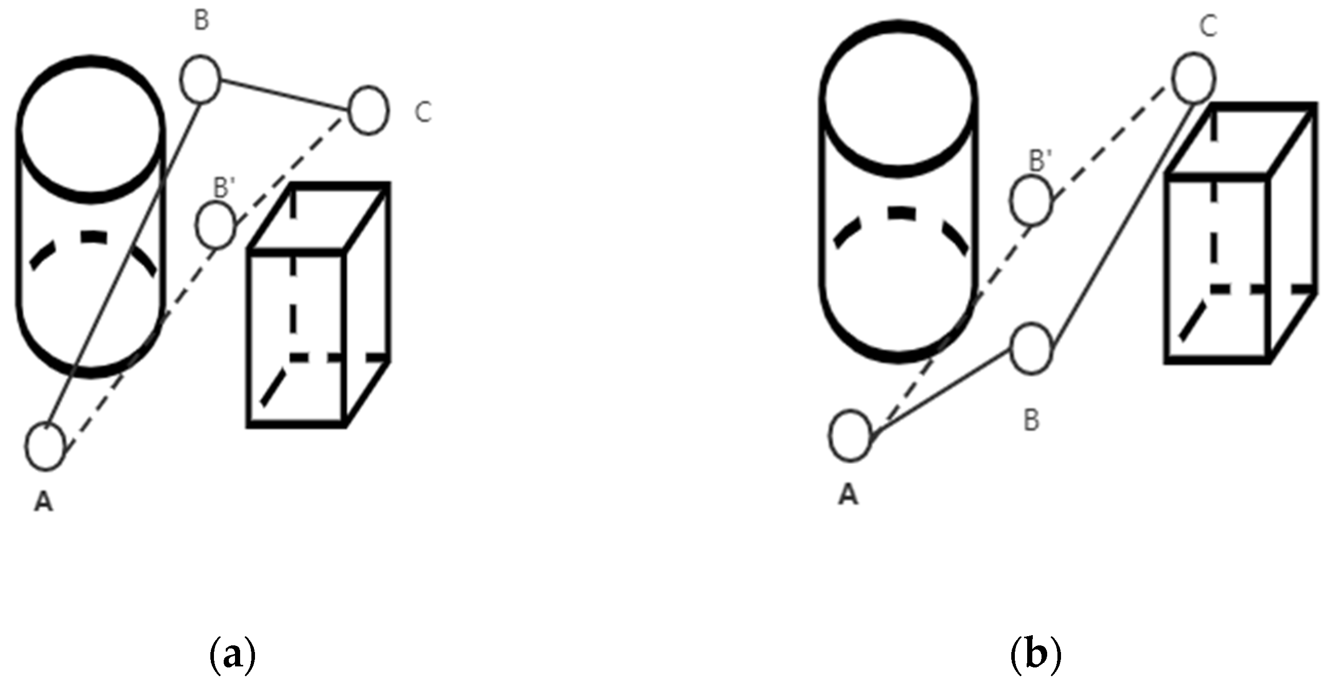
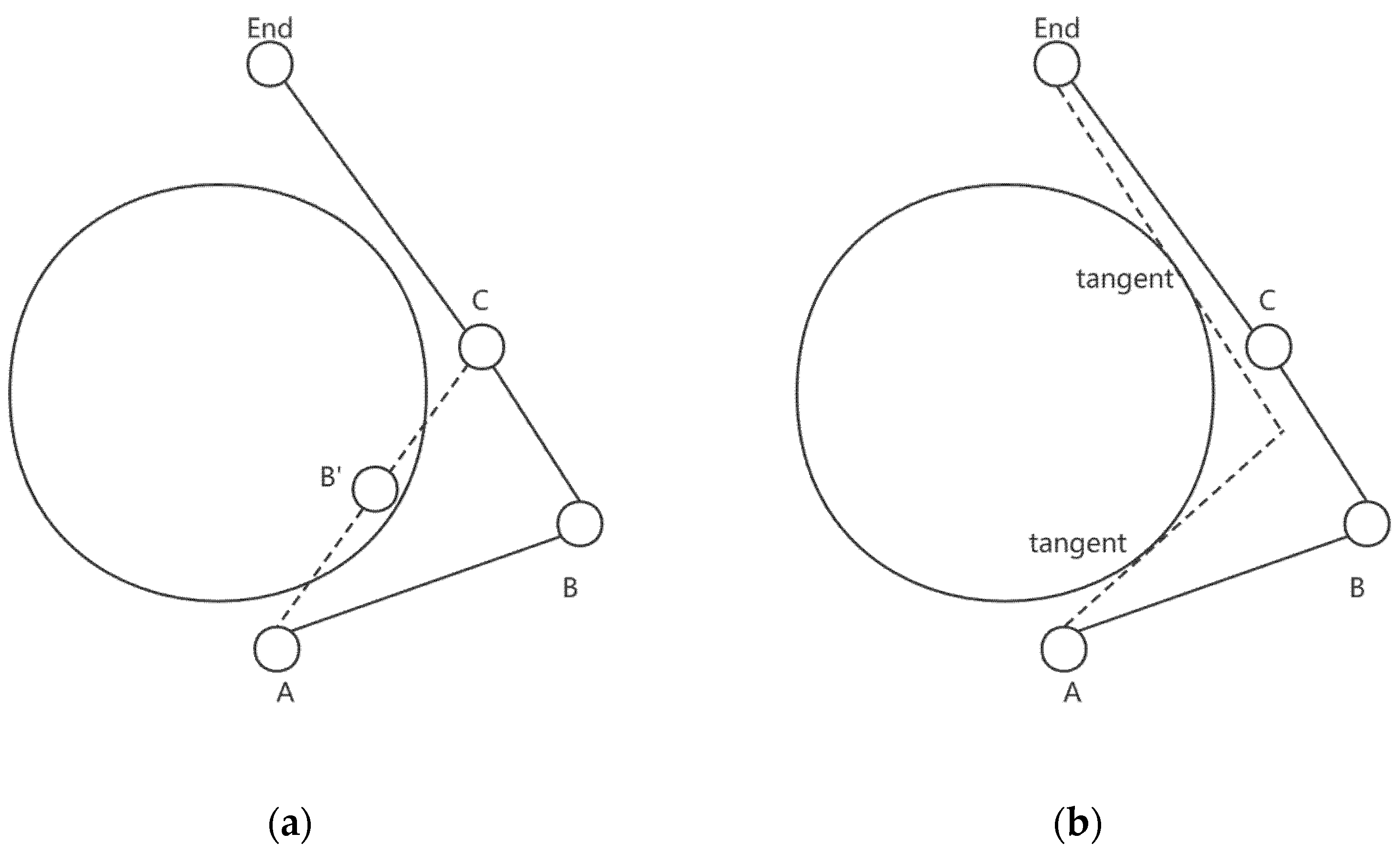
The point of view based on the lines reference point is to find a new point as a preference point on the straight line connecting two adjacent path points. Based on the characteristics of targeted mutation, the newly generated offspring will be located near this preference point. In an ideal situation, the newly generated path points will form a straight line with the adjacent path points, which not only helps to optimize $f_1$ and $f_2$, but also effectively solves the dynamic constraints of the UAV. Because the gliding UAV has the limitation of the minimum steering distance, we chose the middle point of the straight line as the preference point, which is easier to implement. As shown in Figure 3, when the mutation operation is performed on point B, B′ will be selected as a preference point. The calculation method is given in Formula (17).

$$\begin{gathered} x_p=\frac{x_{i,j-1}+x_{i,j+1}}{2} \\ {y}_p=\frac{y_{i,j-1}+y_{i,j+1}}{2} \end{gathered}$$

(17)

2.

Preference points based on no-fly zones

When waypoint $\left(x_{i,j},y_{i,j},z_{i,j}\right)$ violates the Kth no-fly zone restriction, there will be three situations: (1) There is only one individual $l_1$ in the population whose jth waypoint point satisfies the kth no-fly zone constraint, then $\left(x_{l_1,j},y_{l_1,j},z_{l_1,j}\right)$ is selected as the preference point. (2) There are multiple individuals in the population whose jth waypoint satisfies the kth no-fly zone constraint, then randomly select an individual $l_2$ from these individuals, and $\left(x_{l_2,j},y_{l_2,j},z_{l_2,j}\right)$ is selected as the preference point. 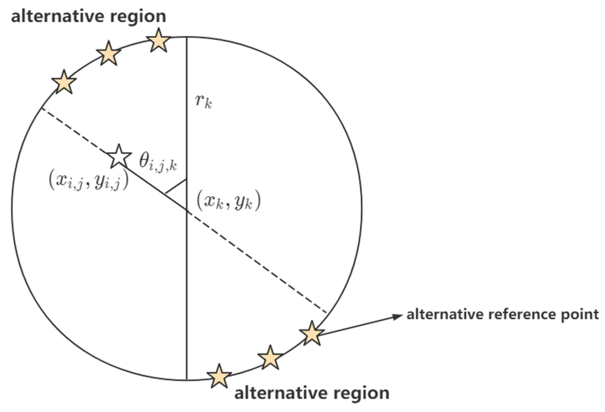(3) If all individuals in the population violate the kth no-fly zone constraint, Formula (18) is used to generate the preference point.

$$\begin{array}{l}if\hspace{0.17em}\hspace{0.17em}rand>0.5\\ x_p=x_k+r_k\times \mathit{cos}(N\left(0,1\right)\times {\theta }_{i,j,k})\\ y_p=y_k+r_k\times \mathit{sin}(N\left(0,1\right)\times {\theta }_{i,j,k})\\ else\\ x_p=x_k+r_k\times \mathit{cos}(\pi +N\left(0,1\right)\times {\theta }_{i,j,k})\\ \hspace{0.17em}\hspace{0.17em}\hspace{0.17em}\hspace{1em}{y}_p=y_k+r_k\times \mathit{sin}(\pi +N\left(0,1\right)\times {\theta }_{i,j,k}).\end{array}$$

(18)

where ${\theta }_{i,j,k}$ is the angle between point $\left(x_{i,j},y_{i,j},z_{i,j}\right)$ and the diameter of the kth no-fly zone. $N\left(0,1\right)$ is the standard normal distribution. As shown in Figure 4, the preference point will be distributed in the alternative region.

3.

Preference points based on terrain

The method of selecting preference points based on terrain restrictions is similar to that of no-fly zone preference points. When the jth waypoint of all individuals in the population violates the terrain constraint, we use Gaussian mutation for waypoint $\left(x_{i,j},y_{i,j},z_{i,j}\right)$ to generate a reference point (as shown in Formula (19)).

$$\begin{gathered} x_p=x_{i,j}+{\sigma }_{i,j}\times N\left(0,1\right) \\ {y}_p=y_{i,j}+{\sigma }_{i,j}\times N\left(0,1\right). \end{gathered}$$

(19)

In this section, we propose three reference point selection methods. Obviously, if three preference point mutations are used at the same time in a targeted mutation operation, the mutation effects of different preference points will cancel each other out. In the multi-stage constraint processing framework of this article, a single mutation operation uses only one method of selecting preference points, and the preference points are selected according to the following rules:

• In the push search stage, only Formula (17) is used to generate preference points.
• In the pull search stage, if and only if the waypoint $\left(x_{i,j},y_{i,j},z_{i,j}\right)$ violates the terrain constraint or no-fly zone constraint, a preference point is generated according to Formula (18) or Formula (19). When two constraints are violated, the preference point based on the no-fly zone is preferred. In other cases, Formula (17) is used to select preference points.

The pseudocode for the generation strategy is listed in Algorithm 3.

Algorithm 3 Offspring generation

Input: $P_T$: Population of the current generation; $P_l$: the Local mutation rate; $PushStage$: Phase transition flag;

Output: The offspring $p$;

1   $p$ $\leftarrow$ Generate a new offspring population by a Single point crossover operator;

2   $q_5$ $\leftarrow$ Update array members;

3   $q_3$ $\leftarrow$ Update array members;

4   $q_5^{\prime }=q_5$; // The backup array of $q_5$

5   $q_3^{\prime }=q_3$; // The backup array of $q_3$

6   $n=N_w\times P_l$; // The number of mutations

7     for $X$ to $p$ do

8         for $i \leftarrow 1$ to $n$ do

9                    $j = \mathrm{randi}\left(2, N_w , 1\right)$; // Randomly select a waypoint

10         if $PushStage==False$ and $X$ not in $q_5^{\prime }\left(j\right)$ then

11                                                                                  // Waypoint $j$ violates no-fly zone constraints

12               $flag=1$;

13               $x_p = \mathrm{Generate} \mathrm{preference} \mathrm{points}\left(q_5 , q_5^{\prime },flag,j,N\right)$;

14               $X^{\prime }\left(j\right)\leftarrow$ Generate a new solution according to Equation (16);

15               $q_5^{\prime }\left(j\right)=q_5^{\prime }\left(j\right){\displaystyle \cup }{X}^{\prime }$; // Update array members

16          else

17               if $PushStage==False$ and $X$ not in $q_3^{\prime }\left(j\right)$ then

18                                                                                  // Waypoint $j$ violates terrain constraints

19                     $flag=0$;

20                    $x_p = \mathrm{Generate} \mathrm{preference} \mathrm{points}\left(q_3 , q_3^{\prime },flag,j,N\right)$;

21                    $X^{\prime }\left(j\right)\leftarrow$ Generate a new solution according to Equation (16);

22                    if $z_j^{\prime }>map\left(x_j^{\prime },y_j^{\prime }\right)+h_{min}$ then

23                             $q_3^{\prime }\left(j\right)=q_3^{\prime }\left(j\right){\displaystyle \cup }{X}^{\prime }$;         // Update array members

24                    end

25               else

26                             $x_p \leftarrow$ Calculate the preference point according to Equation (17);

27                             $X^{\prime }\left(j\right)\leftarrow$ Generate a new solution according to Equation (16);

28              end

29        end

30     end

31  end

In line 7 of Algorithm 1, when calculating the objective function and constraint function of the population, we create two two-dimensional arrays $q_3$ and $q_5$. In array $q_3$, the waypoints that meet the no-fly zone constraint are used as indexes, and individual serial numbers are used as array members. In the array $q_5$, the waypoints satisfying the terrain constraint are used as indexes. In line 10 of Algorithm 3, the selection method of the reference point can be quickly determined according to the created array. Assuming that the 5th, 7th and 10th individuals in the population, the 10th waypoint and the 15th waypoint of these individuals satisfy the constraint functions $c_{10}^3=0$ and $c_{16}^5=0$ respectively, then the two arrays of $q_3$ and $q_5$ are represented as $q_3\left(15\right)=\left\{5,7,10\right\}$ and $q_5\left(16\right)=\left\{5,7,10\right\}$. In line 1 of Algorithm 3, a single-point crossover method is used to generate the offspring population. Since the crossover operation does not change the value of the waypoint, it is unnecessary to recalculate the constraint function of the new individual when updating $q_3$ and $q_5$. At lines 4–5, we created two backup arrays for $q_3$ and $q_5$. In the subsequent mutation operation, individuals in the two arrays $q_3$ and $q_5$ will be preferentially selected as reference points. In line 15 of Algorithm 4, we add new individuals that satisfy the constraints to the backup array instead of the original array. The reason for this is that the new waypoint meets the constraints, but there is no guarantee that the path segment containing the new waypoint meets the constraints. In the line 4 of Algorithm 4, as the number of individuals in the backup array increases, the newly generated individuals will also be selected as reference points to avoid the loss of selection pressure in the population.

Algorithm 4 Generate preference points

Input: $q$: A array of individuals satisfying constraints; $q^{\prime }$: Backup array of $q$; $j$: The sequence number of the waypoint for the mutation operation; $N$: The size of population; $flag$: The flag of Constraint;

Output: $x_p$:Generated reference point;

1  if $flag==1$ then

2                                                                                     // Choose preference points based on no-fly zones

3      if $size\left(q\left(j\right)\right)==0$ then

4               if $rand < exp\left(-3\times size\left(q^{\prime }\left(j\right)\right)÷N\right))$ then

5                      $x_p$ $\leftarrow$ Randomly select an individual from $q^{\prime }\left(j\right)$ as a reference point;

6               else

7                      $x_p$ $\leftarrow$ Calculate the preference point according to Equation (18);

8               end

9      else

10          $x_p$—Randomly select an individual from $q\left(j\right)$ as a reference point;

11      end

12  else

13      if $size\left(q\left(j\right)\right)==0$ then

14                                                                                    // Choose preference points based on terrain

15           if $rand < exp\left(-3\times size\left(q^{\prime }\left(j\right)\right)÷N\right))$ then

16                      $x_p$ $\leftarrow$ Randomly select an individual from $q^{\prime }\left(j\right)$;

17           else

18                      $x_p$ $\leftarrow$ Calculate the preference point according to Equation (19);

19           end

20    else

21           $x_p$ $\leftarrow$ Randomly select an individual from $q^{\prime }\left(j\right)$ as a reference point;

22    end

23 end

2.2.3. Environmental Selection

The proposed algorithm adopts the same environment selection strategy based on adaptive reference point as the ANSGA-III algorithm [13]. Algorithm 5 shows the pseudocode of environment selection.

Algorithm 5 Environmental Selection

Input: $R_T$: New population composed of offspring population and parent population; $\epsilon \left(k\right)$: Population of the current generation; $Z^s$: Reference points; $Z^a$: Desired points; $PushStage$: Phase transition flag;

Output: $P_{T+1}$;

1 $f_{max}$ $\leftarrow$ Maximum fitness of all individuals in $R_t$;

2 for $X$ to $R_T$ do

3     $CV\left(X\right)$ $\leftarrow$ Calculate the total value of constraint violations according to Equation (12);

4      if $PushStage==True$ then

5                                                                                                              // Judgment of no-fly zone restrictions

6             if $g_5\left(X\right)>\epsilon \left(k\right)$ then

7                  $f\left(X\right)=CV\left(X\right)+f_{max}$; // $X$ is an infeasible solution

8             end

9        else

10             if $CV \left(X\right)>\epsilon \left(k\right)$then

11                  $f\left(X\right)=CV\left(X\right)+f_{max}$; // $X$ is an infeasible solution

12             end

13        end

14 end

15 $\left(F_1 , F_2, \dots \right)$ = non-dominated-sort ($R_t$);

16 $S_t=\varnothing$, $i=1$;

17 while $S_t<N$ do

18           $S_t=S_t{\displaystyle \cup }{F}_i$ and $i=i+1$;

19 end

20 if $\left|S_t\right|=N$ then

21           $P_{t+1}=S_t$;

22 else

23 $P_{t+1}= \bigcup _{j=1}^{l-1}{F}_j$;

24  Points to be selected from $F_l$: $K=N-\left|P_{t+1}\right|$;

25 $Z^r$ $\leftarrow$ Normalize objectives and generate reference set;

26 Associate each individual $s$ of $S_t$ with a reference point;

27 $\rho \left(j\right)$ $\leftarrow$ Calculate niche count of reference point $j \in Z^r$;

28 $P_{T+1}$ $\leftarrow$ Select $K$ individuals one at a time from $F_l$ to generate $P_{t+1}$;

29 end

At lines 1 to 14 of Algorithm 5, the principle of feasibility advantage is embedded in Pareto advantage. Specifically, a solution $x_1$ is said to constraint-dominate $x_2$, if: (1) $x_1$ is feasible but $x_2$ is not; (2) $x_1$ and $x_2$ are both infeasible and $CV\left(x_1\right)$ < $CV\left(x_2\right)$; (3) or both of them are feasible and $x_1{\prec }_{Pareto}{x}_2$.

The detailed technology of ANSGA-III based on the adaptive reference point selection mechanism can be found in the corresponding references, namely [13,20]. In this section, this paper briefly describes the principles of environmental selection operations.

In line 14 of Algorithm 5, after the non-dominated solution sorting of the combined population $R_t$ (having $2N$ individuals), all individuals will be assigned to different non-dominated levels ($F_1$, $F_2$, and so on). Next, all individuals in level 1 to $l$ are added to $S_t$. If $S_t=N$; no other actions are required and the next generation is started with $P_{t+1}=St$. For $S_t>N$, the individuals in level 1 to $l-1$ have been chosen, $P_{t+1}= \bigcup _{i=1}^{l-1}{F}_{\mathrm{i}}$, and the rest ($K=N-\left|P_{t+1}\right|$) individuals are selected from the last front $F_l$. After that, normalize the fitness of all individuals in $S_t$ to construct a hyperplane. The reference points whose reference line is nearest to an individual will be associated with the individual. Since the reference points are evenly distributed, when individuals in the new population can be associated with as many reference points as possible, the new population $P_{t+1}$ has better diversity.

NSGA-III requires a set of reference points to be supplied before the algorithm can be applied. A reference line for each reference point can be defined as a line joining the origin and the reference point.in many constrained or even unconstrained problems, not every extended reference line may intersect with the Pareto-optimal front. Thus, there will be some reference points with no Pareto-optimal point associated with them, while others will have more than one point associated with them; hence, NSGA-III may not end up distributing all population members uniformly over the entire Pareto-optimal front. This paper uses the adaptive update reference point mechanism of the ANSGA-III algorithm, and the pseudocode of this mechanism is listed in Algorithm 6. For an M-dimensional constraint problem, at line 1 of Algorithm 6, after creating new population $P_{t+1}$, associate the individuals in the $P_{t+1}$ with the reference point again. In line 5 of Algorithm 1, the distance $L$ between two reference points is calculated. At line 4 of Algorithm 6, find out the reference points associated with over two individuals, and then in the line 9, take these reference points as the center and use a fixed distance $L/2$ to generate $M$ new reference points. After that, delete new reference points that are not in the first quadrant or that are repeated (line 9 and line 14 in Algorithm 6). Finally, delete the new reference point that is not associated with any individual (line 20 in Algorithm 6).

Algorithm 6 Update points

Input: $P_{T+1}$; $Z^s$: Structured points; $l_{distance}:$ The distance between two reference points;

Output: $Z^s$: New reference points;

1 $\rho$ $\leftarrow$ Associate each individual $s$ of $P_{T+1}$ with a reference point;

2 $Z_{temp}=\varnothing$;

3 $P^{\prime }$ $\leftarrow$ The set of reference points where $\rho >2$ in the set $z^s$;

4 while $size\left(P^{\prime }\right)\ne 0$ and $Z_{temp}\ne Z^s$ do

5         $Z_{temp}=Z^s$;

6         for $i$ to $P^{\prime }$ do

7               for $j$ to $M$ do

8                      $p\left(j\right)$ $\leftarrow$ Generate a new reference point with reference point $j$ as the center;

9                               if $p\left(j\right)>0$ then

10                                      $Z^s=\left[Z^s;p\left(j\right)\right]$;

11                              end

12              end

13        end

14 $Z^s$ $\leftarrow$ Delete the repeated reference points in $Z^s$;

15 $\rho$ $\leftarrow$ Update the association of the new reference points $Z^s$;

16 $P^{\prime }$ $\leftarrow$ Update set $P^{\prime }$;

17 end

18 for $i=N+1$ to $Size\left(Z^s\right)$ do

19        if $\rho \left(i\right)==0$ then

20              Remove reference point $i$ from set $Z^s$;

21        end

22 end

2.2.4. Computational Complexity of One Generation of ANSGA-III-PPS

We are given that the population size of the algorithm is $N$, the number of objectives is $M$, the number of constraints is considered to be $\mathrm{G}$, and the number of reference points is H. The computational complexity of the objective function and constraint evaluation (line 6 in Algorithm 1) is $O\left(\left(M+\mathrm{G}\right)\times N\right)$. Calculate the total value of constraint violations in line 12 of Algorithm 1 requires a total of $O\left(N\right)$ computations. Identification of the ideal point and nadir point from lines 10 to 11 of Algorithm 1 requires a total of $O\left(MN\right)$ computations. The computational complexity of update relaxation constraint is $O\left(1\right)$, while the offspring generation is $O\left(N\right)$. Identification of the infeasible solutions in Algorithm 5 requires a total of $O\left(N\right)$ computations. The overall worst-case complexity of one generation of NSGA-III is $O\left(N^{2}lo{g}^{M-2}N\right)$ or $O\left(N^{2}M\right)$, whichever is larger [20]. Line 4 of Algorithm 6 in the worst case requires $O\left(H^{2}M\right)$ computations. In all of our simulations, we have used $N \approx H$, $N>G$ and $N>M$. As a result, the overall computational complexity of ANSGA-III-PPS can be further simplified to $O\left(N^{2}lo{g}^{M-2}N\right)$.

3. Results

In this section, in order to verify the actual capabilities of the proposed algorithm, the proposed algorithm (ANSGA-III-PPS) needs to deal with different obstacle scenarios. We set up three increasingly difficult simulation scenarios. The crucial difference is that the number and range of no-fly zones in each scene were increasing. In each scenario, ANSGA-III-PPS was compared with comparison algorithms with unique characteristics to prove the effectiveness of the three improvement mechanisms proposed in this article. In our performance study, all the path planning algorithms under evaluation are simulated using the MATLAB R2020b simulator. All the results are obtained by repeating thirty times on a windows-10 personal computer with Intel(R) Core I7-9750H 2.6 GHZ CPU and 16 GB memory.

3.1. Scenario Parameters

In the simulation experiment, a simulation scene with an area of 300 km × 300 km × 1.5 km was designed, and the UAV flight mission was a one-way flight. Formulas (2)–(4) are used to generate the terrain threat equivalent map. The original digital terrain parameter settings are shown in

Table 1. Topographic obstacle parameter.

Number	$\mathit{h}$	${\mathit{O}}_1$	${\mathit{O}}_2$	${\mathit{L}}_1$	${\mathit{L}}_2$
1	0.7	50	60	140	20
2	1.75	160	100	170	230
3	1.8	70	30	170	150
4	2.34	130	20	160	190
5	2.5	100	160	280	220
6	3.2	100	100	150	280
7	2.5	175	170	280	220

. In scenario 1, there is no no-fly zone threat, and the search space is large. The optimization ability of the algorithm on the objective function and the processing ability to constraints (flight dynamics constraints and terrain obstacles constraints) were investigated. Scenario 2 and Scenario 3 use the same terrain threat equivalent map as Scenario 1, except that the number of no-fly zones is changed (see

Table 2. No-fly zone parameters.

	No Fly Zone Serial Number	Center Point Coordinates	Radius of Influence
Scenario 1
	N/A	N/A	N/A
Scenario 2
	1	[100,255,0]	50
	2	[240,150,0]	50
	3	[100,100,0]	25
	4	[225,250,0]	25
Scenario 3
	1	[120,240,0]	50
	2	[175,75,0]	50
	3	[225,250,0]	45
	4	[50,175,0]	35
	5	[240,150,0]	35
	6	[75,60,0]	25
	7	[170,170,0]	25
	8	[100,100,0]	25

).

In scenario 2, four no-fly zones were set to limit the search space; in particular, the search space in the area near the straight path, from the start point to the end point, was much smaller than that in the other areas. In scenario 3, eight no-fly zone constraints were set, which further reduced the search space in each area.

3.2. Comparison Algorithms

In order to verify the performance of the proposed algorithm, four representative algorithms were selected: the original algorithm of PPS framework [17]; the MS algorithm [21,22], based on the idea of multi-stage constrained optimization; the ANSGA-III [13] algorithm; and the NSGA-II [23] algorithm, based on crowding distance. The parameters of the comparison algorithm were all set in the original text. The proposed algorithm parameters and public parameters are shown in

Table 3. Algorithm parameters and Public parameters.

Category
Public parameters	$N=100$	$T_{max}=500$	$N_w=20$
	Starting point: [1,1,0.5]	Destination point: [300,300,1]	HV reference point: [3.5,3.5]
	$N_m=5$	${\theta }_{max}={60}^{\circ }$	${\alpha }_{max}={30}^{\circ }$
	$h_{min}=0.5$	$L_{min}=1.5$
ANSGA-III-PPS parameters	$T_c=0.6\times T_{max}$	$\delta =1\times {10}^{-1}$	$cp=2$
	$\alpha =0.95$	$\tau =0.1$	$l=20$
	$F=0.5$	$P_m=0.5$

.

In order to verify the effectiveness of the multi-stage processing strategy proposed in this article in UAV problems with many obstacles, we adopted the generation strategy based on preference points proposed in this article and proposed three varieties of comparison algorithms according to Formulas (16)–(19), MS-PM, ANSGA-III-PM, and NSGA-II-PM.

3.3. Results

There are various performance indicators, such as generational distance (GD), inverted generational distance (IGD), and hypervolume (HV), to measure a given multi-objective evolutionary algorithm (MOEA) [24]. In the UAV path planning problem, the true Pareto front is unknown, so we use the HV as the performance indicator to evaluate the results of the simulation experiment. HV measures the volume of the area in the target space enclosed by the reference point and the non-dominated solution set obtained by the algorithm. The larger the HV value, the better the diversity and convergence of the algorithm.

$$HV=\delta \left(U_{i=1}^{\left|S\right|}{v}_i\right).$$

(20)

In Formula (20), $\delta$ represents the Lebesgue measure, which is used to measure volume. $\left|S\right|$ represents the number of non-dominated solution sets, $v_i$ represents the super volume formed by the reference point and the ith solution in the solution set.

In the problem description in Section 2.1 of this article, we propose to provide a set of Pareto optimal solutions to meet the diverse needs of decision makers. This means that it is difficult to determine which solution is the best before obtaining the preference information of the decision-makers. In this section, in order to objectively reflect the effect of path planning, we use the knee point method to select representative solutions in the non-dominated solution set for display [25]. As shown in Figure 5, these knee solutions are generally characterized as the optimal solutions within the respective regions which can benefit from significant improvement in some objectives at the cost of insignificant degradations in the other objectives from a theoretical perspective. Compared with approaches aggregating weighted objectives into a single fitness function, the knee solutions reflect the optimal solution more accurately without considering multiple preferences of decision-makers [26]. The calculation method of knee point is listed in Formula (21).

$$\begin{gathered} {\mathrm{f}}_{\mathrm{m}}^{\prime }\left(x_i\right)=\frac{{\mathrm{f}}_{\mathrm{m}}\left(x_i\right)- {\overrightarrow{Z}}_m^{*}}{{\overrightarrow{Z}}_m^{nad}-{\overrightarrow{Z}}_m^{*}} \\ \mathrm{V}\left(x_i\right)={\mathrm{f}}_1^{\prime }\left(x_i\right)+{\mathrm{f}}_2^{\prime }\left(x_i\right)+\dots +{\mathrm{f}}_M^{\prime }\left(x_i\right). \end{gathered}$$

(21)

Suppose that there is a non-dominated solution set with $M$ dimensions and $N$ solutions $x_1,x_2,\dots ,x_{ N}$. The nadir point ${\overrightarrow{Z}}^{nad}=\left(Z_1^{nad},Z_1^{nad},\dots ,Z_M^{nad}\right)$ is the maximal objective value among the non-dominated solution set in the $M$ dimensions. Similarly, ${\overrightarrow{Z}}^{*}$ is the minimal objective value among the non-dominated solution set in the $M$ dimensions. Here, ${\overrightarrow{Z}}_m^{*}$ and ${\overrightarrow{Z}}_m^{nad}$ are the best and the worst fitness values found among the whole set of non-dominated solutions in the mth objective space, respectively. For the solution $x_i$ in the non-dominated solution set, when $\mathrm{V}\left(x_i\right)$ is the smallest, the solution $x_i$ is selected as the knee point.

3.3.1. Experimental Results in Scenario 1

In scenario 1, all five comparison algorithms have got feasible solutions, and the results of the HV indicator are shown in

Table 4. Algorithm Comparison Results (scenario 1).

Algorithm	Best	Mean	Worst	Std
ANSGA-III-PPS	0.7308	0.7273	0.7169	0.0035
PPS	0.6817	0.6625	0.5092	0.0303
ANSGA-III-PM	0.7260	0.6736	0.5910	0.0454
NSGA-II-PM	0.6983	0.6681	0.5948	0.0347
MS-PM	0.6589	0.5749	0.4664	0.0547

. The ANSGA-III-PPS algorithm has the best performance, followed by ANSGA-III-PM, and MS algorithm has the worst results. The proposed algorithm and the ANSGA-III-PM algorithm have similar optimal values in scenario 1, but the proposed algorithm has better robustness. In Figure 6, we plot the path of the knee solution when each algorithm obtains the mean HV value, so that the path planning results are most intuitively expressed.

In Figure 6, owing to the larger feasible area, ANSGA-III-PPS and ANSGA-III adopt the same basic framework, and the planned path maintains similar characteristics, but it can be observed that the main difference lies in the ability to continuously optimize the path. Several other algorithms use the way of bypassing obstacles to avoid the influence of terrain constraints. The path height planned by the PPS algorithm varies. In contrast, NSGA-II-PM is smoother, which is consistent so of the HV value.

3.3.2. Experimental Results in Scenario 2

For scenario 2, the results are shown in

Table 5. Algorithm Comparison Results (scenario 2).

Algorithm	Best	Mean	Worst	Std
ANSGA-III-PPS	0.7230	0.7144	0.6518	0.0214
PPS	0.6961	0.6639	0.5892	0.0423
ANSGA-III-PM	0.6502	0.6394	0.6130	0.01
NSGA-II-PM	N/A	N/A	N/A	N/A
MS-PM	N/A	N/A	N/A	N/A

. In scenario 2 increases the number of no-fly zones, which makes the constraints more complicated. Obviously, the advantages of the PPS framework have been reflected. ANSGA-III-PPS has the best performance, followed by the PPS algorithm. Since the constraints of MS-PM and NSGA-II-PM have never been satisfied in all 30 runs, the corresponding HV indicators are recorded as N/A. To the best of our knowledge, the PPS algorithm is the only algorithm that can get feasible solutions without modification.

Figure 7 shows the path planning of the three algorithms.

3.3.3. Experimental Results in Scenario 3

In scenario 3, only two of the five comparison algorithms have successfully completed the path planning task. We showed the results in

Table 6. Algorithm Comparison Results (scenario 3).

Algorithm	Best	Mean	Worst	Std
ANSGA-III-PPS	0.7132	0.7031	0.7011	0.0027
PPS	N/A	N/A	N/A	N/A
ANSGA-III-PM	0.6977	0.6650	0.6511	0.0125
NSGA-II-PM	N/A	N/A	N/A	N/A
MS-PM	N/A	N/A	N/A	N/A

.

The proposed algorithm is still better than the comparison algorithm in scenario 3. As shown in Figure 8, even if there is a large no-fly zone near the destination, the proposed algorithm can effectively avoid it with a smooth path. Comparing the standard deviation of the HV value of the ANSGA-III-PPS algorithm in the three scenarios, in scenario 3, although the obstacles increase, the stability of the ANSGA-III-PPS algorithm is better. For the ANSGA-III-PM algorithm using the same mutation strategy, the performance of scenario 3 is also better than scenario 2.

4. Discussion

In order to further discuss the influence of the various components of the proposed algorithm, in this section we will analyze the various simulation data obtained in the previous section, which will help enrich the research results on this issue.

4.1. The Influence of the Multi-Stage Constraint Processing Framework

In terms of constraint processing, we can divide the five comparison algorithms into two categories. The first category is the synchronization optimization thought represented by MS-PM. MS-PM is also a multi-stage optimization algorithm, but in the first stage of the search process, the method of converting constraints into objective functions is used to achieve the effect of synchronization optimization in the search process.

Other comparison algorithms belong to the second category. They all follow the principle that feasible solutions dominate infeasible solutions [13]. In the scenario of this article, this method has a better path optimization effect.

In scenario 2, the PPS framework showed satisfactory results. The PPS framework represents a method of relaxing constraints, which makes it very different from the ANSGA-III-PM algorithm for identifying feasible solutions.

ANSGA-III uses a similar extreme barrier (EB) method to determine viable solutions. This method helps the algorithm to search in the direction of constraint reduction, but when a feasible solution is found in the population, the individual’s selection pressure will be reduced, which is not conducive to solving complex constraint problems. This strict identification method improves the stability of ANSGA-III in scenarios 2 and 3, but inevitably loses the ability to further optimize. The strict identification method of feasible solutions improves the stability of ANSGA-III in scenario 2 and scenario 3, but inevitably, it also loses the ability to further optimize. In order to better show the difference between the two recognition methods, Figure 9 shows the path of each stage of ANSGA-III-PPS. For the convenience of observation, only the paths of the first 10 individuals in each search behavior stage of the proposed algorithm are drawn.

In Figure 9a, the path points of the population are randomly distributed in the entire search space after initialization. As shown in Figure 9b, at the end of the push search stage, since the preference points based on line (Formula (17)) are selected to guide the search direction of the algorithm, all path points are distributed near the intermediate point. In Section 2.2, we proposed strictly limiting the no-fly zone constraints and using only straight-line-based preference points in the push search stage. The reason is to help quickly construct a line connecting the start and end points and improve the algorithm’s search ability in a narrow area. In addition, the no-fly zones were not all in the preferred point area. As shown in Figure 9b, relying only on the preference points based on lines, the path has successfully avoided most of the no-fly zones. Even at the end of the push search stage, there are some waypoints that violate the no-fly zone restrictions, but owing to the diversity maintenance mechanism, not all waypoints are in the no-fly zone, which also helps to improve the quality of the final solution.

Compare the paths planned by the ANSGA-III-PPS algorithm and the ANSGA-III-PM algorithm in Figure 7b and Figure 9c, respectively. They are similar in the first half. In ANSGA-III-PPS, the relaxation constraint $\epsilon \left(T\right)>0$. Therefore, even if the path collides with the mountain centered at [175,170], the constraint violation of this path is small, and the objective function has good fitness, so the algorithm kept it as a feasible solution. In scenario 2, the result of the original PPS algorithm also proved this point.

4.2. The Influence of the Generation Strategy

It is necessary to compare the proposed mutation operator with DE/rand/1 and DE/rand/best, which are widely used in conventional DE algorithms. The calculation methods of DE/rand/1 and DE/rand/best are listed in Formulas (22) and (23), respectively.

$${\overrightarrow{v}}_i={\overrightarrow{x}}_{r1}+F\times {\overrightarrow{x}}_{r2}-{\overrightarrow{x}}_{r3}.$$

(22)

$${\overrightarrow{v}}_i={\overrightarrow{x}}_{best}+F\times {\overrightarrow{x}}_{r1}-{\overrightarrow{x}}_{r2}.$$

(23)

where ${\overrightarrow{x}}_{r1}$, ${\overrightarrow{x}}_{r2}$, ${\overrightarrow{x}}_{r3}$ are three distinct individuals that are randomly selected from the current population, $F$ is a scale factor, and ${\overrightarrow{x}}_{best}$ is the best individual in the current population. In DE/rand/1, the viewpoint of random search is adopted, which helps to jump out of the local optimum. In DE/rand/best, the search for the best solution direction is emphasized, which helps to speed up the convergence speed.

To investigate the mechanism behind the proposed mutation operator, a series of experiments have been performed. The proposed mutation operator is replaced by the DE/rand/1 and DE/rand/best. The algorithm with DE/rand/1 is named the ANSGA-III -PPS-DE. In the multi-objective optimization algorithm, we cannot find a true global optimal solution as the basis vector of the DE/rand/best operator. In the literature [25], a DE/rand/best operator with knee points instead of the global optimal solution is proposed. Therefore, the algorithm with DE/rand/best is named the ANSGA-III -PPS-KNEE. The statistical results of HV values obtained by the proposed mutation strategy and the other two mutation strategies are shown in

Table 7. Statistical results of mutation operator in terms of performance indicators HV.

Algorithm	Best	Mean	Worst	Std
Scenario 2
ANSGA-III-PPS	0.7230	0.7144	0.6518	0.0214
ANSGA-III -PPS-DE	0.6914	0.6555	0.6072	0.0351
ANSGA-III -PPS-KNEE	0.6367	0.6288	0.6136	0.0131
Scenario 3
ANSGA-III-PPS	0.7132	0.7031	0.7011	0.0027
ANSGA-III -PPS-DE	0.6680	0.6386	0.5228	0.0450
ANSGA-III -PPS-KNEE	0.6498	0.6498	0.6498	0

.

In Table 7, the HV value of the proposed mutation strategy is better than the other two comparison strategies. From the Pareto-optimal front of the three mutation strategies in Figure 10, we can see that the convergence of the proposed mutation strategy is better than the other two comparative mutation strategies. In Figure 11, the proposed mutation strategy significantly improves the success rate of the algorithm solution. At the end of the push search stage, there are many waypoints in the population that violate terrain constraints and no-fly zone constraints. The mutation operator DE/rand/1 provides no search direction to optimize these constraints, and the optimal solution selected by the mutation operator DE/rand/best is the knee point obtained under the premise of only the no-fly zone constraints. The original PPS algorithm uses the DE/rand/1, but in Scenario 3, no feasible solution is got. However, after using the same DE/rand/1 in ANSGA-III-PPS, the effect is second only to the proposed strategy. We believe one reasons for this difference is that the crossover operation can better preserve the advantages of the path segment [27].

In the past, researchers have focused on generating strategies to find helpful feasible waypoints that do not violate constraints to guide the generation of offspring. However, the generation strategy proposed in this paper is the opposite. We first adopted the greedy idea to construct low-altitude linear paths as much as possible during the push search stage. These paths would largely violate terrain constraints and no-fly zone constraints. Therefore, in the pull search stage, the generation strategy focuses on optimizing these two types of constraints. As shown in Figure 12, by relaxing the constraint mechanism and using the mutation strategy based on preference points to construct a straight line that intersects with obstacles, we can continuously adjust the position of waypoints to get better solutions.

5. Conclusions

This paper proposes an improved algorithm ANSGA-III-PPS based on a multi-stage constraint processing strategy to solve the problem of UAV trajectory planning in a 3D environment. Aiming at the characteristics of evolutionary algorithms for handling UAV obstacle avoidance constraints, we introduced the PPS constraint processing framework combined with mutation strategies to effectively improve the algorithm’s ability to solve problems and prevent the algorithm from falling into a local optimal situation prematurely. The experimental results show that the ANSGA-III-PPS algorithm has advantages in the ability and robustness to solve the UAV path planning problem with many obstacles.

This research provides some ideas for the problems of large search space and difficulty in handling constraints in UAV trajectory planning. With advancements in drone technology, the application scenarios of drones have become more diversified, and the research on heterogeneous drone swarms has also become a hot spot. In the follow-up research, we will also strengthen the research of heterogeneous fleet scheduling, and build a complete solution from UAV scheduling to route optimization. On the other hand, the performance study of different generation strategies in UAV path planning will also be our focus in the future.

References

1. Aggarwal, S.; Kumar, N. Path planning techniques for unmanned aerial vehicles: A review, solutions, and challenges. Comput. Commun. 2020, 149, 270–299. [Google Scholar] [CrossRef]
2. Chen, H.; Wang, X.-M.; Li, Y. A Survey of Autonomous Control for UAV. In Proceedings of the 2009 International Conference on Artificial Intelligence and Computational Intelligence, Shanghai, China, 7–8 November 2009; pp. 267–271. [Google Scholar]
3. Zhao, Y.; Zheng, Z.; Liu, Y. Survey on computational-intelligence-based UAV path planning. Knowl.-Based Syst. 2018, 158, 54–64. [Google Scholar] [CrossRef]
4. Radmanesh, M.; Kumar, M.; Guentert, P.H.; Sarim, M. Overview of Path-Planning and Obstacle Avoidance Algorithms for UAVs: A Comparative Study. Unmanned Syst. 2018, 6, 95–118. [Google Scholar] [CrossRef]
5. Ma, Y.; Hu, M.; Yan, X. Multi-objective path planning for unmanned surface vehicle with currents effects. ISA Trans. 2018, 75, 137–156. [Google Scholar] [CrossRef] [PubMed]
6. Qu, C.; Gai, W.; Zhong, M.; Zhang, J. A novel reinforcement learning based grey wolf optimizer algorithm for unmanned aerial vehicles (UAVs) path planning. Appl. Soft Comput. 2020, 89, 106099. [Google Scholar] [CrossRef]
7. Li, Z.; Zeng, Y.; Wang, Y.; Wang, L.; Song, B. A hybrid multi-mechanism optimization approach for the payload packing design of a satellite module. Appl. Soft Comput. 2016, 45, 11–26. [Google Scholar] [CrossRef]
8. Golabi, M.; Ghambari, S.; Lepagnot, J.; Jourdan, L.; Brévilliers, M.; Idoumghar, L. Bypassing or flying above the obstacles? A novel multi-objective UAV path planning problem. In Proceedings of the 2020 IEEE Congress on Evolutionary Computation (CEC), Glasgow, UK, 19–24 July 2020; pp. 1–8. [Google Scholar]
9. Gálvez, J.; Cuevas, E.; Becerra, H.; Avalos, O. A hybrid optimization approach based on clustering and chaotic sequences. Int. J. Mach. Learn. Cybern. 2019, 11, 359–401. [Google Scholar] [CrossRef]
10. Roberge, V.; Tarbouchi, M.; Labonte, G. Comparison of Parallel Genetic Algorithm and Particle Swarm Optimization for Real-Time UAV Path Planning. IEEE Trans. Ind. Inform. 2013, 9, 132–141. [Google Scholar] [CrossRef]
11. Yang, P.; Tang, K.; Lozano, J.A.; Cao, X. Path Planning for Single Unmanned Aerial Vehicle by Separately Evolving Waypoints. IEEE Trans. Robot. 2015, 31, 1130–1146. [Google Scholar] [CrossRef] [Green Version]
12. Zhang, X.; Duan, H. An improved constrained differential evolution algorithm for unmanned aerial vehicle global route planning. Appl. Soft Comput. 2015, 26, 270–284. [Google Scholar] [CrossRef]
13. Jain, H.; Deb, K. An Evolutionary Many-Objective Optimization Algorithm Using Reference-Point Based Nondominated Sorting Approach, Part II: Handling Constraints and Extending to an Adaptive Approach. IEEE Trans. Evol. Comput. 2014, 18, 602–622. [Google Scholar] [CrossRef]
14. Cheng, Z.; Li, D. Improved GASA algorithm for mutation strategy UAV path planning. In Proceedings of the 2018 10th International Conference on Communication Software and Networks (ICCSN), Chengdu, China, 6–9 July 2018; pp. 506–510. [Google Scholar]
15. Poudel, S.; Moh, S. Hybrid Path Planning for Efficient Data Collection in UAV-Aided WSNs for Emergency Applications. Sensors 2021, 21, 2839. [Google Scholar] [CrossRef] [PubMed]
16. Zhang, H.; Wang, S.; Liu, T.; Zhou, A.; Zhang, Y. Optimization of Missile Path Planning Based on APMO-HV Algorithm. In Proceedings of the 2019 IEEE International Conference on Unmanned Systems (ICUS), Palermo, Italy, 29–31 October 2019; pp. 495–501. [Google Scholar]
17. Fan, Z.; Li, W.; Cai, X.; Li, H.; Wei, C.; Zhang, Q.; Deb, K.; Goodman, E. Push and pull search for solving constrained multi-objective optimization problems. Swarm Evol. Comput. 2019, 44, 665–679. [Google Scholar] [CrossRef] [Green Version]
18. Audet, C.; Dennis, J.E. A Progressive Barrier for Derivative-Free Nonlinear Programming. SIAM J. Optim. 2009, 20, 445–472. [Google Scholar] [CrossRef] [Green Version]
19. Zheng, W.; Fu, H.; Yang, G. Targeted Mutation: A Novel Mutation Strategy for Differential Evolution. In Proceedings of the 2015 IEEE 27th International Conference on Tools with Artificial Intelligence (ICTAI), Vietri sul Mare, Italy, 9–11 November 2015; pp. 286–293. [Google Scholar]
20. Deb, K.; Jain, H. An Evolutionary Many-Objective Optimization Algorithm Using Reference-Point-Based Nondominated Sorting Approach, Part I: Solving Problems With Box Constraints. IEEE Trans. Evol. Comput. 2014, 18, 577–601. [Google Scholar] [CrossRef]
21. Tian, Y.; Zhang, Y.; Su, Y.; Zhang, X.; Tan, K.C.; Jin, Y. Balancing Objective Optimization and Constraint Satisfaction in Constrained Evolutionary Multiobjective Optimization. IEEE Trans. Cybern. 2021. [Google Scholar] [CrossRef] [PubMed]
22. Tian, Y.; Cheng, R.; Zhang, X.; Jin, Y. PlatEMO: A MATLAB platform for evolutionary multi-objective optimization [educational forum]. IEEE Comput. Intell. Mag. 2017, 12, 73–87. [Google Scholar] [CrossRef] [Green Version]
23. Deb, K.; Pratap, A.; Agarwal, S.; Meyarivan, T. A fast and elitist multiobjective genetic algorithm: NSGA-II. IEEE Trans. Evol. Comput. 2002, 6, 182–197. [Google Scholar] [CrossRef] [Green Version]
24. Yen, G.G.; He, Z. Performance Metric Ensemble for Multiobjective Evolutionary Algorithms. IEEE Trans. Evol. Comput. 2014, 18, 131–144. [Google Scholar] [CrossRef]
25. Yu, X.; Li, C.; Yen, G.G. A knee-guided differential evolution algorithm for unmanned aerial vehicle path planning in disaster management. Appl. Soft Comput. 2021, 98, 106857. [Google Scholar] [CrossRef]
26. Zou, F.; Yen, G.G.; Tang, L. A knee-guided prediction approach for dynamic multi-objective optimization. Inf. Sci. 2020, 509, 193–209. [Google Scholar] [CrossRef]
27. Sun, X.; Wang, Y.; Kang, H.; Shen, Y.; Chen, Q.; Wang, D. Modified Multi-Crossover Operator NSGA-III for Solving Low Carbon Flexible Job Shop Scheduling Problem. Processes 2021, 9, 62. [Google Scholar] [CrossRef]
Figure 1. Examples of sampling points to detect no-fly zones ( N m = 5 ).
Drones 05 00144 g001
Figure 2. Schematic diagram of constraint processing in the push search stage. (a) Initialization of the population and (b) End of the push search phase.
Drones 05 00144 g002
Figure 3. (a) Bypass the obstacle in case 1 and (b) Bypass the obstacle in case 2 (side view).
Drones 05 00144 g003
Figure 4. Preference point selection for the no-fly zone.
Drones 05 00144 g004
Figure 5. Example of the knee point ( M = 2 ).
Drones 05 00144 g005
Figure 6. Side view of the path planned by 5 algorithms (scenario 1). (a) ANSGA-III-PPS, (b) ANSGA-III -PM, (c) PPS, (d) NSGA-II-PM and (e) MS-PM.
Drones 05 00144 g006aDrones 05 00144 g006b
Figure 7. Top view of the path planned by 3 algorithms (scenario 2). (a) ANSGA-III-PPS, (b) ANSGA-III-PM and (c) PPS.
Drones 05 00144 g007
Figure 8. (a,b) are the top view and side view of the route planned by ANSGA-III-PPS in scenario 3, respectively. (c,d) are the top view and side view of the path planned by ANSGA-III-PM in scenario 3, respectively.
Drones 05 00144 g008
Figure 9. ANSGA-III-PPS path planning at each stage (N = 10) (scenario 2). (a) The initial path of the population. (b) The planned path at the end of the push search phase. (c) The planning path when the number of iterations T is equal to the maximum relaxation generation T c .
Drones 05 00144 g009
Figure 10. (a,b) are the Pareto-optimal frontiers of ANSGA-III-PPS, ANSGA-III-PPS-DE and ANSGA-III-PPS-KNEE in scenario 2 and scenario 3, respectively.
Drones 05 00144 g010
Figure 11. The number of successful runs of ANSGA-III-PPS, ANSGA-III-PPS-DE and ANSGA-III-PPS-KNEE (30 runs).
Drones 05 00144 g011
Figure 12. (a) Generate strategy to bypass the no-fly zone schematic diagram (top view). (b) Bypass the no-fly zone optimal path (top view).
Drones 05 00144 g012