Abstract
For safe UAV navigation and to avoid collision, it is essential to have accurate and real-time perception of the environment surrounding the UAV, such as free area detection and recognition of dynamic and static obstacles. The perception system of the UAV needs to recognize information such as the position and velocity of all objects in the surrounding local area regardless of the type of object. At the same time, a probability based representation taking into account the noise of the sensor is also essential. In addition, a software design with efficient memory usage and operation time is required in consideration of the hardware limitations of the UAVs. In this paper, we propose a 3D Local Dynamic Map (LDM) generation algorithm for a perception system for UAVs. The proposed LDM uses a circular buffer as a data structure to ensure low memory usage and fast operation speed. A probability based occupancy map is created using sensor data and the position and velocity of each object are calculated through clustering between grid voxels using the occupancy map and velocity estimation based on a particle filter. The objects are predicted using the position and velocity of each object and this is reflected in the occupancy map. This process is continuously repeated and the flying environment of the UAV can be expressed in a three-dimensional grid map and the state of each object. For the evaluation of the proposed LDM, we constructed simulation environments and the UAV for outdoor flying. As an evaluation factor, the occupancy grid is accuracy evaluated and the ground truth velocity and the estimated velocity are compared.
1. Introduction
In recent years, the use of unmanned aerial vehicles (UAVs) has increased significantly in various fields, including surveillance, agriculture, transportation, rescue and military [1,2,3,4,5]. Accordingly, for safe UAV navigation that avoids collisions, research on perception of flight environments such as object detection, tracking and mapping are actively conducted [6,7,8,9,10]. For planning and control for safe UAV navigation and accurate and real-time perception of the surrounding environment such as occupied and free areas, dynamic and static obstacles are essential. We believe that the following three are essential considerations for the perception system for safe navigation of UAVs.
- It is necessary to know the state such as the position and velocity of all objects existing in a local area around the UAV regardless of the type of object. When the UAV is flying, it is necessary to distinguish between places where collisions may occur and not. Further, in the case of dynamic objects, we need to predict the motion of objects and avoid them. Therefore, the current position and velocity of objects in the surrounding 3D local area of a UAV are essential factors that must be recognized.
- Probabilistic representation of the surrounding environment which, considering the noise of the sensor, is needed. We can recognize the surrounding environment through sensors such as LiDAR, camera and radar. However, since sensor data always has noise, it must be expressed as a probabilistic expression that considers sensor noise like sensor noise models. This can further be useful for integrating different sensors.
- The limit of hardware systems of UAVs should be considered when configuring a UAV’s perception system. Compared to other mobility platforms, UAVs have a relatively limited payload weight. Due to this, the usable sensors and computing boards are limited. Therefore, we need to build a software with efficient memory and execution time within the limited hardware situation.
As a perception system, Occupancy Grid Map (OGM) represents an environment by using probabilistic grid cells. OGMs discretize the space into grid cell space to improve memory efficiency and represent the occupancy probability of each cell by using a sensor noise model. Reference [9] extended this to 3D space and made it possible to apply OGM for UAVs. However, since most OGMs are used as a prior map of wide areas for the purpose of global mapping or SLAM, it could not be guaranteed that memory usage and computation time are used in real time. As UAVs have limited hardware specifications that can be implemented, we need to reduce memory usage and computational load by limiting the perception area to only the adjacent surrounding area of the UAV. Reference [11] proposed an occupancy grid map using a circular buffer for this purpose. The occupancy map of [11] is limited only for a local area around the current UAV location for efficiency and it is suitable for UAVs. However, it is still regrettable that [11] does not have object-level expressions such as the position and velocity of each object, which are useful for navigation.
Most object-level perception algorithms are based on a deep learning approach such as in [10,12,13]. In recent years, many studies have been continuously conducted and object recognition and classification have been performed using camera and LiDAR. However, deep learning based algorithms can recognize only pre-trained objects. In the case of autonomous vehicles, the objects that can appear on the road are limited, but since UAVs do not have the concept of a driving road, a wide variety of objects can appear, so it is difficult to fully recognize the surrounding environment only with a deep learning approach. In addition, it requires vast amounts of training data, but UAVs’ flying data is insufficient, making it difficult to apply. Therefore, an additional method is needed and OGMs are appropriate for a perception system for collision avoidance navigation of UAVs.
As mentioned above, the limitation of OGM is no representation of the object-level state. So, OGMs that contain object-level representation can break the limitation and Occupancy Grid Filter (OGF) algorithms such as in [14,15,16] are most suited to this purpose. OGF expresses the occupancy and velocity of each cell as a probability. Furthermore, references [17,18] calculated the position and velocity of each object cluster through clustering and tracking between cells. However, these algorithms are studied for autonomous vehicles so they are conducted in 2D space. For UAVs, reference [19] expresses even the dynamic situation by utilizing the Bin-occupancy filter for the local area around the UAV, but the computational load is heavy.
In summary, the previous perception algorithms for safe navigation of UAVs have limitations in the way of expression and the types of objects that can be recognized. OGM algorithms such as [9,11] are not designed to express object-level expressions such as object velocity, size and position. On the other hand, deep learning approaches such as in [10,12,13] were able to express the object level, but could only recognize learned objects and did not show grid-level expression using occupancy probability. In addition, most of the OGF algorithms do not target UAVs, so they are limited to the 2D domain and some algorithms for UAVs have high computational costs, making it difficult to apply them in real time. In this paper, to solve the problems of these previous algorithms, we propose an algorithm to generate a Local Dynamic Map (LDM) that includes a 3D voxel grid map, object clusters and particle set. LDMs that are generated by the proposed algorithm can express the UAV flying environment in two ways, grid-level and object-level, so that there is no limit to the path planning and collision avoidance algorithms that can be used in conjunction. In order to reduce used memory and computation time, we use a circular buffer data structure from [11]. The occupancy probability of each voxel in a grid map is predicted by using the previous state of object clusters and is updated by using the sensor measurement of the current time. Using this voxel grid map, the occupied area and velocity of each object are obtained through particle filter based velocity estimation and clustering. We evaluate the occupancy grid accuracy of the proposed LDM algorithm with the one used in [11]. The state of objects such as position and velocity are compared with the ground truth in the simulation. In addition, it is also tested and evaluated using an outdoor UAV composed of LiDAR sensor and onboard PC.
2. Related Works
OGM is an algorithm that represents the surrounding environment for safe navigation. Various sensors such as a sonar sensor, LiDAR and RGB-D camera are used and applied to various platforms such as mobile robot and autonomous vehicle [20,21,22,23,24]. However, these OGMs express the environment in two dimensions; reference [9] makes a 3D grid map by using an octree data structure to reduce memory usage and computation time. References [25,26] use an Octomap as a perception system for 3D navigation of UAVs. However, OGMs have weaknesses in update speed and prediction for dynamic objects because they accumulate measurements and show only the occupancy probability of the current state.
Reference [14] proposed one of the OGFs, Bayesian Occupancy Filter (BOF), which extended OGM to a 4D-grid that consists of velocity probabilities of each occupancy grid cell to compensate for the weaknesses of an OGM that can only consider occupancy. In BOF, the state of each cell is predicted using the previous occupancy and velocity probability. Through this, a corresponding grid map is created for dynamic objects, but there is an inefficient aspect of having a velocity grid for all cells including free cells.
References [15,16] applied a particle filter to BOF to solve the above inefficient problem and expressed the velocity of each cell as particle distribution. In addition, the cell was divided into static, dynamic and free and the efficiency of calculation was improved by allocating and removing particles.
The aforementioned OGF algorithms express the occupancy probability and velocity of a grid cell, but these are all two-dimensional representations and are not suitable for 3D navigation of UAVs. Reference [19] created a 3D grid map for a local area around the UAV to avoid collision based on the Bin-occupancy filter which predicts the movement of particles in each cell. However, it is limited in use due to insufficient evaluation of the accuracy of mapping and the heavy computational load. References [27,28] use a Euclidean Signed Distance Fields (ESDFs) grid map as a 3D representation for UAV navigation. These obtain the shortest distance to the occupied voxel and obtains the possible collision distance in real time. However, these algorithms have no representation of velocity field or object state so the trajectory of dynamic objects cannot be predicted.
Reference [11] proposed an algorithm that creates a circular buffer based local grid map for UAV replanning. The data structure of the occupancy grid is a circular buffer to reduce computation time. We take the circular buffer data structure proposed by [11] for our proposed LDM. However, unlike [11], we perform the occupancy prediction process to respond to dynamic objects.
Clustering of occupancy grid has been proposed for a planning technique that uses object recognition information. In [29], the states of grid cells are determined through comparison between cell occupancy probability of the current and previous time and cell clustering is applied using these states. Reference [18] projected the clustering result from the superpixel approach, which uses the pixel clustering algorithm, to grid space and assign the clusters to each cell. Reference [17] applied clustering and tracking between cells using the BOF grid.
3. Local Dynamic Map (LDM) Generation
We propose an algorithm for Local Dynamic Map (LDM) generation that expresses the surrounding environment by occupancy grid and obstacle clusters. The proposed algorithm represents the space occupied by obstacles in the local area around the UAV as the occupancy grid and at the same time recognizes the states of obstacles such as position and velocity. The occupancy grid is predicted by using the previous state of objects and is updated by using sensor measurement of current time. To extract the obstacle state, LDM uses grid voxel clustering and particle filter based velocity of cluster estimation.
As shown in Figure 1, the overall process proceeds in the order of prediction, update, resampling and clustering. The prediction step predicts the movement of close objects based on the LDM of previous time step, time in Figure 1. This process is divided into occupancy prediction, which predicts the occupancy grid map state and particle prediction, which predicts the particle state. After that, the update step, which reflects the current flying environment information of the UAV, is performed. It is divided into three steps: Movement update, occupancy update and particle update. The movement update step updates the grid map region of LDM by using the current position of the UAV. This step removes the area away from the LDM due to the movement of the UAV and initializes the area that is newly close to the UAV. Occupancy update is the process of reflecting distance sensor measurements such as LiDAR mounted on the UAV to the 3D voxel grid map of the LDM. This process can determine whether each voxel in the LDM is currently occupied by objects. The particle update step is the process of updating the particle state using the voxel grid map in the LDM. Each particle’s weight is updated using the occupancy probability of the voxel in which each particle is located. This is a process to get a difference in the reliability of the position and velocity information of each particle. After that, the resampling step adjusts the overall number of particles based on weight. The clustering process generates object clusters by using occupancy probability to provide object-level representation. In the next time segment, time in Figure 1, the prediction and update steps are performed recursively by using object clusters and particle states of . In this section, the prediction, update, resampling and clustering steps are described in detail.
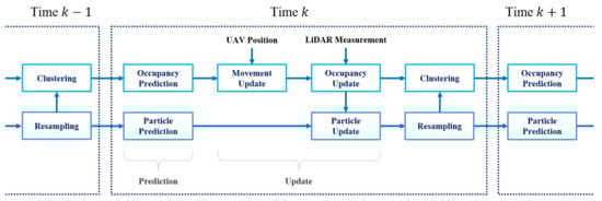
Figure 1.
An overview of the proposed local dynamic map algorithm.
3.1. LDM State Representation
Before explaining each step of the proposed algorithm, we summarize the composition and state of LDM. LDM consists of a 3D voxel grid map representing the local area of the UAV, a set of object clusters and a set of particles freely present in the grid map region. Each voxel of the grid map stores an occupancy probability, which is a probability that the corresponding voxel area is occupied. Object clusters are created for object-level representation of the flight environment and it has position and velocity as the state of each cluster. Particles play a role in estimating the moving velocity of objects in the grid map region. The state of each particle consists of position, velocity and weight.
In LDM, the environment around the UAV is divided into a 3D grid composed of voxels. Each voxel in the form of a cube expresses occupancy and dynamic state by using the occupancy probability and velocity. Occupancy probability is stored as log-odds notation as shown in Equation (1) for computational benefits.
where is log-odds notation of voxel i and is its occupancy probability.
In order to recognize only the local area around the UAV, the grid map region continuously moves based on the location of the UAV. The easiest way to do this is to match the center of the grid map region with the location of the UAV. However, this requires an occupancy probability update process for whole voxels every time the UAV moves. In most cases, the accuracy of occupancy probability may be lost due to overlap between voxels. To prevent this, we update the grid map region so that the UAV is located only inside the center grid voxel of the map. Due to the movement of UAVs, if the UAV located voxel moves , where are multiples of voxel resolution from the previous UAV located voxel (same as the center grid voxel), the grid map region moves by the same distance so that the UAV located voxel becomes the center grid voxel. Moreover, the rotation of the grid map due to the rotation of the UAV is not considered and the orientation of the map is fixed as the orientation of the initial. Therefore, since the grid map region moves only in multiples of the voxel resolution, the overlap between voxels can be blocked. Figure 2 describes this with an example situation.
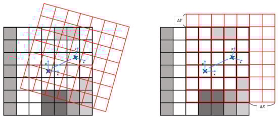
Figure 2.
An example of the update process of the grid map in the proposed LDM. For visualization, we reduce the dimension to 2D. On the left is the example of the overlap situation when the update grid map region depends on UAV position and orientation. The right image is the update process used in our LDM. If the UAV located voxel moves as shown in the right image, the grid map region also moves . LDM prevents overlap issues by using this updated process.
The estimated velocity of each voxel is expressed as a set of particles. The particles have their position and velocity. To represent the reliability of the particle’s position and velocity, each particle has a weight. The representation of the particle state is:
where is the position of particle i and is the velocity of particle i. Obstacles can move randomly; so we have to predict the probability of the movement in all possible directions. Therefore, we use weighted particles as a probability of the obstacle state to recognize the velocity and position of each obstacle.
The particles of the LDM are initialized so that they are evenly distributed over the entire grid map region. So the particle i, is in uniform distribution over the grid map region with being the size of the grid map region. The velocity of particle i, is normal distribution with covariance . The weight of each particle, , is set to the same value.
3.2. Prediction
Because traditional occupancy grid measurement update methods such as [9,11] are based on accumulation of measurements, the reaction of the dynamic obstacles is slow in a dynamic environment. To prevent this, occupancy prediction is applied using the clustering result. Through the clustering to be described in Section 3.5, we collected the clusters with their corresponding voxels and the velocity of clusters. By using this, the current moving position of the clusters are predicted and the corresponding occupancy probability can be predicted as described in Figure 3.
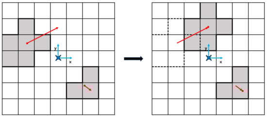
Figure 3.
Example of occupancy prediction. The gray color cells are occupied cells and the part where the border is drawn with a thick line is one cluster. In left image, red dots are the position of each cluster, red arrows are the velocity of each cluster. The end of the arrow is the predicted position of each cluster. In this case the left upper cluster is predicted to the right upper direction and the right lower cluster is predicted to the right lower direction. The occupancy probabilities are moved according to the same direction of clusters.
Particles distributed over the grid map region are predicted using the prediction model from [16].
where is the time difference between time k and time , is the zero mean normal distribution noise with covariance . If the predicted location of the particle is outside the grid map, it is removed and is not used in the subsequent process.
3.3. Update
3.3.1. Movement Update
We use the circular buffer data structure of [11] for our grid map data structure. It is composed of a circular buffer array that stores the occupancy probability of each voxel in 3D grid space and offsets voxel , indicating the grid voxel that corresponds to the first index of the circular buffer array. To update the grid map region, the offset voxel is updated using Equation (6).
with means grid voxel where the UAV located at time k relative to grid voxel coordinate at time and means the offset voxel at time k. In this process, voxels that move out of the grid map region are cleaned and voxels that are included newly to the grid map region are initialized. To do this simply and fast, circular buffer indexes of the moved out voxels are allocated to newly entered voxels and initialized to log-odds notation of unknown probability, as shown in Figure 4. Through this, the grid map update according to the movement of the UAV can be performed with high speed.
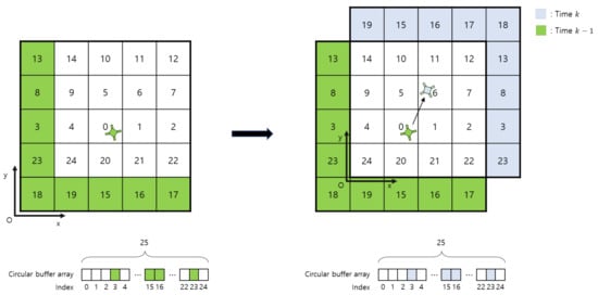
Figure 4.
Movement update process. For visualization, we reduce the dimension to two dimensions. The number of each voxel is the index of the circular buffer array. At time , the voxel with the index of the circular buffer equal to 18 is the origin voxel of the grid voxel coordinate. The offset voxel and where the UAV is located. At time k, after the UAV moved, the voxel where the UAV located relative to the grid voxel coordinate at time . The offset voxel is updated as . Now the voxel with the index of the circular buffer equal to 24 is the origin voxel of the grid voxel coordinate. By update offset and grid voxel coordinate, the voxels in the green zone are now out of the grid map region and voxels in the blue zones have newly entered the grid map region. To reduce the time used by data update, the circular buffer array indexes of green zone voxels such as 3, 15, 16 and 23 are allocated to blue zone voxels with 0 value.
3.3.2. Occupancy Update
We use 3D-LiDAR, which provides point measurements with low noise compared to vision and radar sensors, to recognize the surrounding environment of the UAV. In order to update measurements to the occupancy grid, a measurement flag grid of the same size as the occupancy grid is created to indicate the presence or absence of measurement of each voxel. In the the measurement flag grid, the voxel with the measurement is marked as occupied. We apply the ray-casting algorithm to the occupied voxels and voxels that pass by rays are marked as free.
For each voxel of the occupancy grid, the occupancy probability is updated by using the marking of the measurement flag grid. Since we use log-odds notations, we can simplify update Equations (7) and (8).
where is measurement at time k, is predicted occupancy probability of voxel i at time k, is occupancy probability posterior to voxel i at time k and means measurement probability. The equation is:
where and are constant parameters and it is recommended to set to more than 0.5 and to less than 0.5.
Some voxels may not have any flags due to the influence of sensing field of view or interference from other objects. In a dynamic environment, concerning voxels without sensor information it could not be guaranteed that the previous occupancy probability was reasonable for the present occupancy probability. Therefore, the LDM that we proposed updates these voxels using the survival probability so that the influence of the previous occupancy probability gradually decreases over time. Now we update voxels that do not have any flags by using Equation (10).
where, is survival probability that the state of voxel i can remain. If a lot of time passes without sensor measurement, log-odds notation of occupancy probability of voxel converges to 0, which is the middle of the free and occupied state.
Survival probability is set differently for each voxel in consideration of occupancy grid of time and flag grid of current time. Voxels that do not have any flags are divided into three cases: First, the voxels that are occupied by a static object at time. In this case, it can be said that the occupancy probability of these voxels is the same as before because they are occupied by the same object even after time passes. Therefore, if the velocity of a voxel at time is less than the threshold velocity, it is determined that the voxel is occupied by a static object and the is set to 1.
Except for the above case, voxels can be divided into the case where they are located outside the sensor range and the part of the voxels where they are inside the sensor range but interfered with by other objects. In the former case, the current situation is unknown due to the hardware limitation of the sensor, so all voxels in this case have the same . In the latter case, different is determined according to the distance from the object causing the interference. The distance close to the interfering object is more likely to be occupied by the object due to the effect of the object’s thickness, motion, etc., but this decreases as the distance increases. Therefore, for voxels passing by extending the ray between the voxel occupied by the interference object (same as occupied flag voxel) and the sensor origin to the end of the map, voxels at a certain distance from the occupied flag voxel have high and subsequent voxels are set so that decreases in inverse proportion to the distance.
3.3.3. Particle Update
The reliability of the prediction of the particle is high if the occupancy probability of the voxel that the predicted particle is located is high. Therefore, the weight of the particle is updated using the occupancy probability updated to the current measurement. The particle update equation is:
where is the weight of particle i at time k and j is the index of the voxel where particle i is located.
We can express the state of the voxel using particles. The velocity of each voxel is expressed as the weighted average of particles in each voxel:
where means velocity of voxel j, n is the number of particles in voxel j and is the velocity of particle i. In this process, some occupied voxels may not be properly updated due to the insufficient number of particles. Therefore, to prevent this, add particles to occupied voxels where not enough particles are located. The position of new particles, (, r is voxel resolution) is uniformly distributed within the voxel and the velocity is:
where is zero mean normal distribution noise with covariance . The weight of each particle, is set as where j is the voxel where particle i is located.
The last part of the update process, the weight of the particles are normalized and the equation is:
where is the normalization factor with:
where N is the number of total particles.
3.4. Resampling
The total number of particles has changed due to particle deletion or addition through the prediction and update process. Therefore, to keep the number of particles the same as the initial state, the resampling process is essential. The resampling sequence is as follows. First, a discrete distribution is created based on the weight of particles and a particle is randomly selected using this distribution and added to the new particle array. This is done until the size of the new array becomes , which is the initial number of particles. Through this, particles can be selected in proportion to the weight and therefore more particles can be placed in occupied voxels.
3.5. Voxel Clustering
Objects with different states are clustered using the occupancy probability of the voxels. We consider the connectivity between 26-neighborhood voxels for only voxels with an occupancy probability higher than the threshold. The position of each cluster is expressed as the average value of the voxels included in the cluster. The velocity of each cluster is expressed as the weighted average of particles existing in the cluster,
where is the velocity of cluster j at time k; n is the number of particles in cluster j. From this process, the grid voxels included in each cluster and the velocity of the cluster are obtained.
After clustering, particles located in the clusters additionally adjust the velocity. We can know the velocity of each cluster, grid voxels and particles corresponding to the cluster. Among the resampled particles, they are located in the same cluster, but the velocity can be very different. Therefore, the velocity of these particles is readjusted using the velocity of the cluster. The equation is:
where is the velocity of cluster j where particle i is located.
4. Evaluation
To evaluate the LDM algorithm, we built a testbed in both simulation and outdoor UAV with LiDAR sensor. Occupancy grid and estimated velocity accuracy is evaluated in various scenarios.
4.1. Simulation
4.1.1. Experimental Setup
The simulation constructed a virtual environment using the V-REP simulator. We created a number of static and dynamic objects in a virtual space and constructed a virtual UAV equipped with 3D LiDAR. The LDM algorithm is implemented with a C++ based ROS node. The UAV position, orientation and LiDAR sensor data of the V-REP are communicated to the LDM algorithm node as an ROS topic using the V-REP-ROS communication node. The parameters for the proposed LDM algorithm are initialized before activation of the UAV. , which is the initial number of the particles is set to 200,000, the resolution of voxel is set to and the number of grid voxels is 32,768 (32). and are set in the same manner as in [9,11].
To evaluate the occupancy probability and estimated velocity of LDM, we generated the corresponding ground truth values. For evaluation of the scenarios in which dynamic obstacles exist, a ground truth grid map is created based on the current position of the obstacle for every time. By comparing the occupancy probability with this, we define an evaluation indicator:
where is the number of voxels matched to the same state ({occupied, free}) by comparing ground truth and occupancy grid of LDM, D is the number of voxels at onetime step and t is the value of the time step. We also know the ground truth velocity of each object in the simulation, so we compared this value with the estimated velocity of each cluster.
We created various scenarios with dynamic and static obstacles through simulation and measured the accuracy of the LDM algorithm. The scenarios are:
- : Dynamic obstacles and UAV flying
- : Static obstacles and UAV flying
- : Dynamic and static obstacles and UAV flying
these are describe in Figure 5. In these scenarios, we ignore the ground measurement.
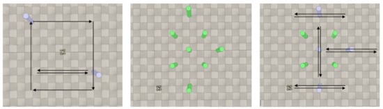
Figure 5.
Simulation scenarios. Left image is scenario 1, middle image is scenario 2 and right image is scenario 3. The blue obstacles are static obstacles and green obstacles are static obstacles. The black arrows are the trajectory of the dynamic obstacles.
4.1.2. Occupancy Grid Accuracy
We evaluate the occupancy grid accuracy of the proposed LDM and the circular buffer based grid map in [11]. We also measure the number of false expressed voxels divided into two cases. Case 1 means that the ground truth is occupied but expressed as free and case 2 means that the ground truth is free but expressed as occupied.
Compared with [11], the proposed LDM predicts the occupancy probability by using the velocity of clusters and Table 1 shows the effect of these approaches. In scenario 1 where there are dynamic obstacles, the number of case 1 and case 2 false voxels of the proposed algorithm is less than that in [11]. This is because the accumulation of the occupancy probabilities continued more rapidly by the prediction of the occupancy probability using the predicted velocity of the dynamic obstacle. Therefore, the proposed algorithm provides a more accurate representation of free space by the decrease in the number of case 1 false voxels and also represents the occupied space better.

Table 1.
Occupancy grid accuracy of each scenario. The number of case1 false voxels means the number of false expressed voxels where the ground truth is occupied but expressed as free. The number of case 2 false voxels means the number of false expressed voxels where the ground truth is free but expressed as occupied.
In scenario 2, which is composed of only static obstacles, the accuracy of the proposed algorithm is slightly lower. The proposed algorithm applies the survival probability to voxels without measurement due to object interference or sensor field of view. On the other hand, reference [11] keeps the previous occupancy probability of the unobserved voxels. Therefore, it can be seen that [11] is more advantageous in a static environment, but it is not appropriate to say that it is advantageous even in general scenarios involving dynamic obstacles such as scenario 3 because the accuracy of the proposed algorithm is slightly higher. The average of the total computation time of the proposed LDM is 98 ms.
4.1.3. Velocity Estimation
To evaluate the estimated velocity from the proposed algorithm, we compared the velocity of dynamic and static obstacles with the ground truth. There are many algorithms that estimate the velocity in the 2D grid, but in the 3D grid there is no velocity estimation with voxels for the local grid map. So we used a method that applied the particle filter based velocity estimation part of our proposed algorithm to the occupancy grid map of [11] as a comparison algorithm of the proposed algorithm and this is expressed as in [11] with the PF (Particle Filter) in this evaluation.
Figure 6 shows the absolute value of the estimated velocity error of a static obstacle. The velocity estimation of the proposed algorithm is more accurate for static obstacles in almost all times compared to [11] with PF. The average velocity error of the proposed algorithm is m/s, while [11] with PF showed an average velocity error of m/s.
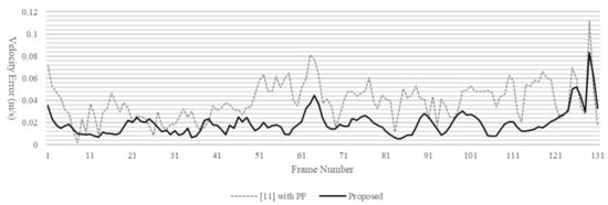
Figure 6.
Estimated velocity error of static obstacle. The dotted line is [11] with PF method and the solid line is the proposed LDM generation algorithm.
Figure 7, Figure 8 and Figure 9 show the result of velocity estimation of a dynamic obstacle. The measured obstacle moved only the x and y directions. The time for the estimated velocity to reach the ground truth velocity of the dynamic obstacle is similar between the proposed LDM and [11] with PF. However, in the case of [11] with PF, the estimated velocity is not constant, whereas in the case of the proposed LDM, the estimated velocity is almost similar to the ground truth velocity and is estimated at a constant. The average velocity error of the proposed LDM is m/s, while [11] with PF shows m/s average velocity error.
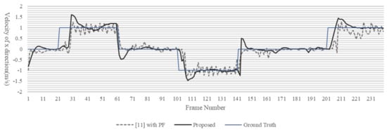
Figure 7.
Estimated x direction velocity and ground truth velocity of the dynamic obstacle. The dotted line is [11] with PF method, the black solid line is the proposed LDM generation algorithm and the blue solid line is the ground truth.
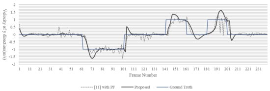
Figure 8.
Estimated y direction velocity and ground truth velocity of the dynamic obstacle. The dotted line is [11] with PF method, the black solid line is the proposed LDM generation algorithm and the blue solid line is the ground truth.
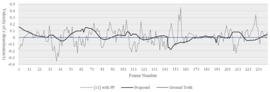
Figure 9.
Estimated z direction velocity and ground truth velocity of the dynamic obstacle. The dotted line is [11] with PF method, the black solid line is proposed LDM generation algorithm and the blue solid line is the ground truth.
4.2. Outdoor UAV Experiment
4.2.1. Experimental Setup
We implement the hardware and software system for outdoor UAV to evaluate the proposed LDM algorithm. as shown in Figure 10. As the body frame, Matrice 100, which includes GPS, IMU and flight controller, is used. Ouster 16-channel 3D LiDAR is used as a sensor to recognize the flying environment. Jetson TX2 board is used to acquire sensor data and run the algorithm and an extra battery is additionally installed to operate the board. The proposed LDM algorithm implementation is the same as the simulation’s one. The evaluation is conducted in two scenarios. Scenario 1 is a scenario consisting of two moving people and one stationary person and scenario 2 is a situation where the UAV and the person move in the same direction as shown in Figure 11.
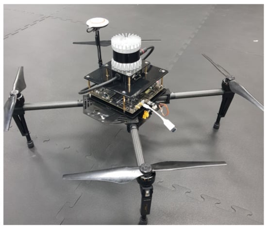
Figure 10.
The structure of the implemented UAV.
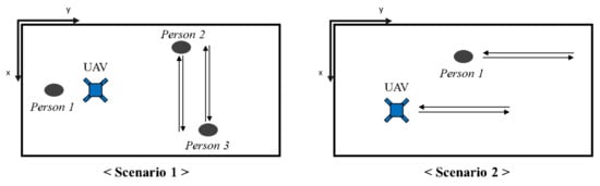
Figure 11.
Scenarios of outdoor UAV experiment. In scenario 1, the UAV is stopped and there are three people. In scenario 2, the UAV and one person move in the same direction.
4.2.2. Experiment Results
The results of the proposed LDM are shown in Figure 12 and Figure 13. In Figure 12, for the experiment, we created an environment with one static obstacle (Person1) and two dynamic obstacles (Person2 and Person3). Among the dynamic obstacles, Person2 moves to Person3 ( direction) and Person3 moves to Person2 ( direction). When each reaches the other’s starting position, they come back to their own starting position. Interference of Person3 by Person2 occurs in image 3 in Figure 12, but the cluster is not lost because of occupancy prediction. It can be seen that the velocity direction is estimated according to the moving direction of the dynamic objects.
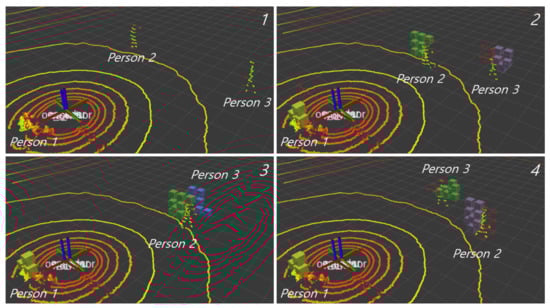
Figure 12.
Subfigures of the proposed LDM for scenario 1 of the outdoor UAV experiment. The number of each subfigure represents the passage of time. Person1 is a static obstacle that does not move, Person2 and Person3 are moved to each other. The colored points represent LiDAR measurements and only occupied voxels among all voxels are visualized. The color of each voxel means the cluster number and the direction of the velocity of each voxel is marked with a red arrow.
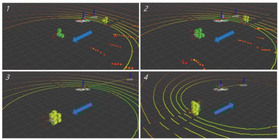
Figure 13.
Subfigures of the proposed LDM for scenario 2 of the outdoor UAV experiment with the dynamic obstacle. The number of each subfigure represents the passage of time. In this scenario, the UAV and the obstacle are moving in the same direction and the big blue arrow is the direction of the UAV and the obstacle. The colored points represent LiDAR measurements and only occupied voxels among all voxels are visualized. The color of each voxel means the cluster number and the direction of the velocity of each voxel is marked with a red arrow.
Figure 14, Figure 15 and Figure 16 show the velocity, estimated by the proposed LDM, of obstacles in the scenario of Figure 12. Figure 14 is the estimated velocity of the static obstacle (Person1). The proposed LDM shows an error of up to 0.05 m/s in all directions for the estimated velocity of a static obstacle. Figure 15 represents the estimated velocity of Person2 and Figure 16 represents the estimated velocity of Person3. From 91 to 181 frames, when Person2 moves in the direction, we can see that Person3 moves in the direction. It can also be seen that after frame 181, these peoples return to their starting points.
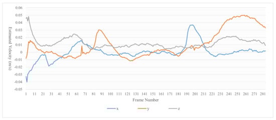
Figure 14.
Estimated velocity of the static obstacle (Person1) in Figure 12.
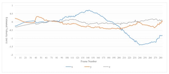
Figure 15.
Estimated velocity of the dynamic obstacle that started at the upper left (Person2) in Figure 12.
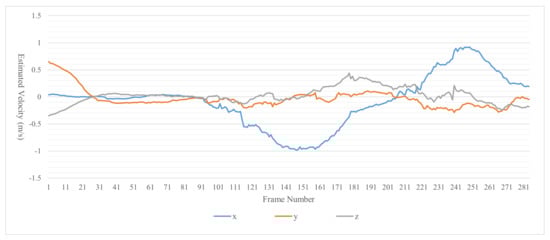
Figure 16.
Estimated velocity of the dynamic obstacle that started at the lower right (Person3) in Figure 12.
Figure 13 shows another scenario testing the proposed LDM and its results. In this scenario, the UAV and an obstacle are moving in the same direction always. In images 1–3 of Figure 13, the UAV is moved to the direction and the obstacle is also moved in the same direction. In image 4 of Figure 13, the UAV is moved to the direction and the obstacle is also moved. We can see that the direction of the obstacle and the direction of the estimated velocity of the obstacle are the same.
5. Conclusions
In this paper, we proposed an LDM generation algorithm that expresses the surrounding environment of the UAV with a 3D occupancy grid and the object clusters in real time. The proposed LDM represents the local area around the UAV as a circular buffer based occupancy grid to reduce computational cost. To extract object-level state information such as velocity and position of object clusters, we use grid voxel clustering and particle filter based velocity estimation. We evaluated the performance of the proposed algorithm through simulations and real world experiments. The results showed that the proposed algorithm can estimate the velocity of an object with less error while exhibiting mapping accuracy similar to that of the grid map in [11]. In addition, object-level expression is also provided through clustering, enabling connection with various planning algorithms. Finally, the proposed algorithm satisfied three considerations for the UAV perception system mentioned in Section 1.
In the future, the algorithm that we proposed will be used together with the planning and control algorithm to form an integrated UAV system capable of collision avoidance flying. Because the computation time of the proposed algorithm may increase when the map size and the number of particles are increased, we plan to address this issue through parallel programming and optimization of the algorithm.
Author Contributions
Conceptualization, J.-W.L. and K.-D.K.; Data curation, W.L.; Formal analysis, J.-W.L. and W.L.; Investigation, J.-W.L.; Methodology, J.-W.L.; Project administration, K.-D.K.; Software, J.-W.L. and W.L.; Supervision, K.-D.K.; Visualization, J.-W.L. and W.L.; Writing—original draft, J.-W.L.; Writing—review & editing, J.-W.L. and K.-D.K. All authors have read and agreed to the published version of the manuscript.
Funding
This work was supported by the DGIST R&D Program of the Ministry of Science and ICT (21-CoE-IT-01).
Institutional Review Board Statement
Not applicable.
Informed Consent Statement
Not applicable.
Conflicts of Interest
The authors declare no conflict of interest.
References
- Alotaibi, E.T.; Alqefari, S.S.; Koubaa, A. Lsar: Multi-uav collaboration for search and rescue missions. IEEE Access 2019, 7, 55817–55832. [Google Scholar] [CrossRef]
- Tisdale, J.; Kim, Z.; Hedrick, J.K. Autonomous UAV path planning and estimation. IEEE Robot. Autom. Mag. 2009, 16, 35–42. [Google Scholar] [CrossRef]
- Pretto, A.; Aravecchia, S.; Burgard, W.; Chebrolu, N.; Dornhege, C.; Falck, T.; Fleckenstein, F.; Fontenla, A.; Imperoli, M.; Khanna, R.; et al. Building an Aerial-Ground Robotics System for Precision Farming: An Adaptable Solution. arXiv 2019, arXiv:1911.03098. [Google Scholar] [CrossRef]
- Brunner, G.; Szebedy, B.; Tanner, S.; Wattenhofer, R. The urban last mile problem: Autonomous drone delivery to your balcony. In Proceedings of the 2019 International Conference on Unmanned Aircraft Systems (Icuas), Atlanta, GA, USA, 11–14 June 2019; pp. 1005–1012. [Google Scholar]
- Condomines, J.P. Nonlinear Kalman Filter for Multi-Sensor Navigation of Unmanned Aerial Vehicles: Application to Guidance and Navigation of Unmanned Aerial Vehicles Flying in a Complex Environment; Elsevier: Amsterdam, The Netherlands, 2018. [Google Scholar]
- Saha, S.; Natraj, A.; Waharte, S. A real-time monocular vision-based frontal obstacle detection and avoidance for low cost UAVs in GPS denied environment. In Proceedings of the 2014 IEEE International Conference on Aerospace Electronics and Remote Sensing Technology, Yogyakarta, Indonesia, 13–14 November 2014; pp. 189–195. [Google Scholar]
- Stegagno, P.; Basile, M.; Bülthoff, H.H.; Franchi, A. A semi-autonomous UAV platform for indoor remote operation with visual and haptic feedback. In Proceedings of the 2014 IEEE International Conference on Robotics and Automation (ICRA), Hong Kong, China, 31 May–7 June 2014; pp. 3862–3869. [Google Scholar]
- Florence, P.R.; Carter, J.; Ware, J.; Tedrake, R. Nanomap: Fast, uncertainty-aware proximity queries with lazy search over local 3d data. In Proceedings of the 2018 IEEE International Conference on Robotics and Automation (ICRA), Brisbane, Australia, 21–25 May 2018; pp. 7631–7638. [Google Scholar]
- Hornung, A.; Wurm, K.M.; Bennewitz, M.; Stachniss, C.; Burgard, W. OctoMap: An efficient probabilistic 3D mapping framework based on octrees. Auton. Robot. 2013, 34, 189–206. [Google Scholar] [CrossRef] [Green Version]
- Ammour, N.; Alhichri, H.; Bazi, Y.; Benjdira, B.; Alajlan, N.; Zuair, M. Deep learning approach for car detection in UAV imagery. Remote Sens. 2017, 9, 312. [Google Scholar] [CrossRef] [Green Version]
- Usenko, V.; Von Stumberg, L.; Pangercic, A.; Cremers, D. Real-time trajectory replanning for MAVs using uniform B-splines and a 3D circular buffer. In Proceedings of the 2017 IEEE/RSJ International Conference on Intelligent Robots and Systems (IROS), Vancouver, BC, Canada, 24–28 September 2017; pp. 215–222. [Google Scholar]
- Rahman, M.M.; Tan, Y.; Xue, J.; Lu, K. Recent advances in 3D object detection in the era of deep neural networks: A survey. IEEE Trans. Image Process. 2019, 29, 2947–2962. [Google Scholar] [CrossRef]
- Fraga-Lamas, P.; Ramos, L.; Mondéjar-Guerra, V.; Fernández-Caramés, T.M. A review on IoT deep learning UAV systems for autonomous obstacle detection and collision avoidance. Remote Sens. 2019, 11, 2144. [Google Scholar] [CrossRef] [Green Version]
- Coué, C.; Pradalier, C.; Laugier, C.; Fraichard, T.; Bessière, P. Bayesian occupancy filtering for multitarget tracking: An automotive application. Int. J. Robot. Res. 2006, 25, 19–30. [Google Scholar] [CrossRef] [Green Version]
- Nuss, D.; Yuan, T.; Krehl, G.; Stuebler, M.; Reuter, S.; Dietmayer, K. Fusion of laser and radar sensor data with a sequential Monte Carlo Bayesian occupancy filter. In Proceedings of the 2015 IEEE Intelligent Vehicles Symposium (IV), Seoul, Korea, 28 June–1 July 2015; pp. 1074–1081. [Google Scholar]
- Nègre, A.; Rummelhard, L.; Laugier, C. Hybrid sampling bayesian occupancy filter. In Proceedings of the 2014 IEEE Intelligent Vehicles Symposium Proceedings, Dearborn, MI, USA, 8–11 June 2014; pp. 1307–1312. [Google Scholar]
- Mekhnacha, K.; Mao, Y.; Raulo, D.; Laugier, C. Bayesian occupancy filter based “fast clustering-tracking” algorithm. In Proceedings of the IROS, Nice, France, 22–26 September 2008. [Google Scholar]
- Oh, S.I.; Kang, H.B. Fast occupancy grid filtering using grid cell clusters from LIDAR and stereo vision sensor data. IEEE Sens. J. 2016, 16, 7258–7266. [Google Scholar] [CrossRef]
- Odelga, M.; Stegagno, P.; Bülthoff, H.H. Obstacle detection, tracking and avoidance for a teleoperated UAV. In Proceedings of the 2016 IEEE international conference on robotics and automation (ICRA), Stockholm, Sweden, 16–21 May 2016; pp. 2984–2990. [Google Scholar]
- Lu, D.V.; Hershberger, D.; Smart, W.D. Layered costmaps for context-sensitive navigation. In Proceedings of the 2014 IEEE/RSJ International Conference on Intelligent Robots and Systems, Chicago, IL, USA, 14–18 September 2014; pp. 709–715. [Google Scholar]
- Kato, S.; Tokunaga, S.; Maruyama, Y.; Maeda, S.; Hirabayashi, M.; Kitsukawa, Y.; Monrroy, A.; Ando, T.; Fujii, Y.; Azumi, T. Autoware on board: Enabling autonomous vehicles with embedded systems. In Proceedings of the 2018 ACM/IEEE 9th International Conference on Cyber-Physical Systems (ICCPS), Porto, Portugal, 11–13 April 2018; pp. 287–296. [Google Scholar]
- Matthies, L.; Elfes, A. Integration of sonar and stereo range data using a grid-based representation. In Proceedings of the 1988 IEEE International Conference on Robotics and Automation, Philadelphia, PA, USA, 24–29 April 1988; pp. 727–733. [Google Scholar]
- Shvets, E.; Shepelev, D.; Nikolaev, D. Occupancy grid mapping with the use of a forward sonar model by gradient descent. J. Commun. Technol. Electron. 2016, 61, 1474–1480. [Google Scholar] [CrossRef]
- Homm, F.; Kaempchen, N.; Ota, J.; Burschka, D. Efficient occupancy grid computation on the GPU with lidar and radar for road boundary detection. In Proceedings of the 2010 IEEE Intelligent Vehicles Symposium, La Jolla, CA, USA, 21–24 June 2010; pp. 1006–1013. [Google Scholar]
- Mittal, M.; Mohan, R.; Burgard, W.; Valada, A. Vision-based autonomous UAV navigation and landing for urban search and rescue. arXiv 2019, arXiv:1906.01304. [Google Scholar]
- Vanegas, F.; Gaston, K.J.; Roberts, J.; Gonzalez, F. A framework for UAV navigation and exploration in GPS-denied environments. In Proceedings of the 2019 IEEE Aerospace Conference, Big Sky, MT, USA, 2–9 March 2019; pp. 1–6. [Google Scholar]
- Oleynikova, H.; Taylor, Z.; Fehr, M.; Siegwart, R.; Nieto, J. Voxblox: Incremental 3d euclidean signed distance fields for on-board mav planning. In Proceedings of the 2017 IEEE/RSJ International Conference on Intelligent Robots and Systems (IROS), Vancouver, BC, Canada, 24–28 September 2017; pp. 1366–1373. [Google Scholar]
- Han, L.; Gao, F.; Zhou, B.; Shen, S. Fiesta: Fast incremental euclidean distance fields for online motion planning of aerial robots. arXiv 2019, arXiv:1903.02144. [Google Scholar]
- Bouzouraa, M.E.; Hofmann, U. Fusion of occupancy grid mapping and model based object tracking for driver assistance systems using laser and radar sensors. In Proceedings of the 2010 IEEE Intelligent Vehicles Symposium, La Jolla, CA, USA, 21–24 June 2010; pp. 294–300. [Google Scholar]
Publisher’s Note: MDPI stays neutral with regard to jurisdictional claims in published maps and institutional affiliations. |
© 2021 by the authors. Licensee MDPI, Basel, Switzerland. This article is an open access article distributed under the terms and conditions of the Creative Commons Attribution (CC BY) license (https://creativecommons.org/licenses/by/4.0/).