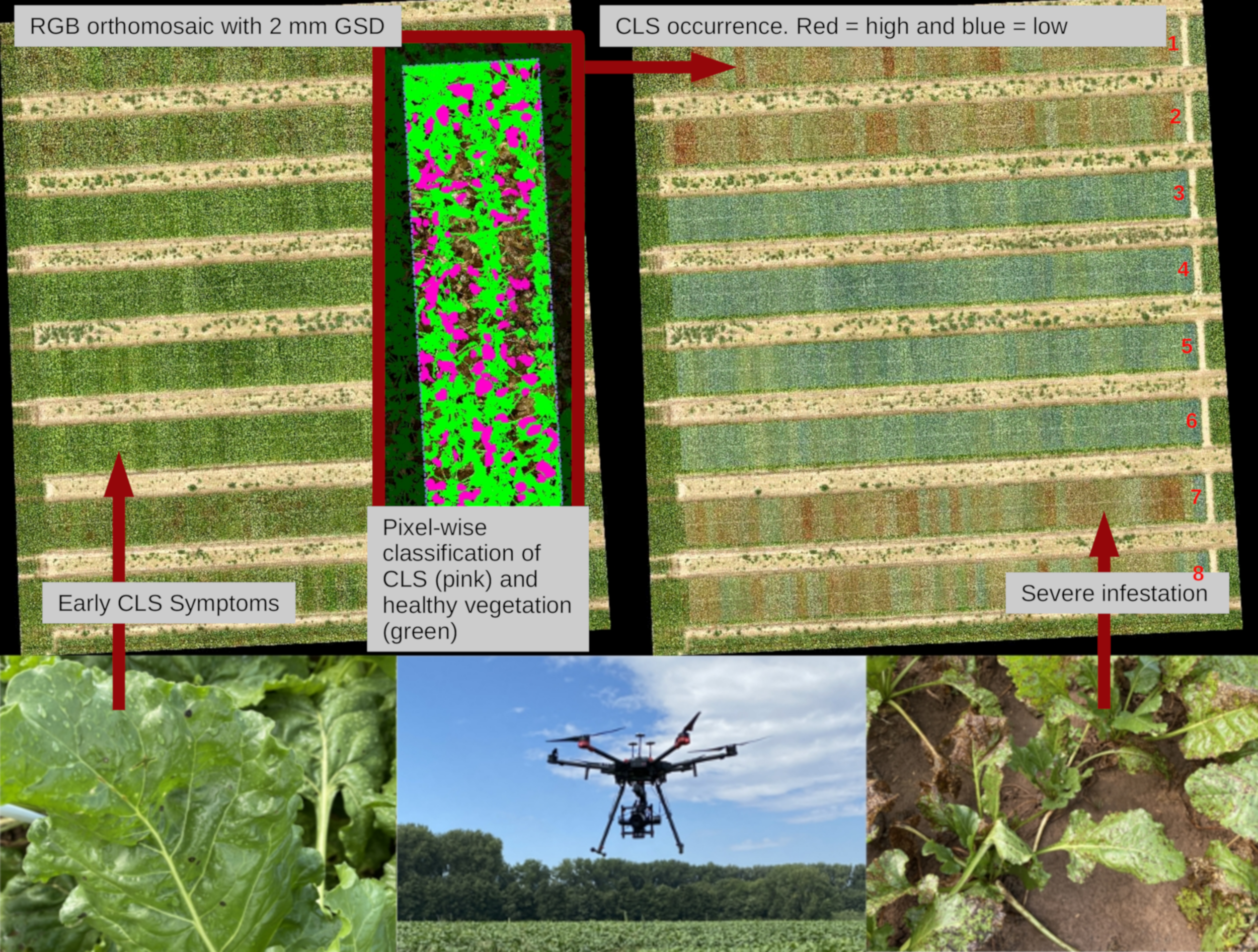
UAV-Based Classification of Cercospora Leaf Spot Using RGB Images

Abstract

Plant diseases can impact crop yield. Thus, the detection of plant diseases using sensors that can be mounted on aerial vehicles is in the interest of farmers to support decision-making in integrated pest management and to breeders for selecting tolerant or resistant genotypes. This paper investigated the detection of Cercospora leaf spot (CLS), caused by Cercospora beticola in sugar beet using RGB imagery. We proposed an approach to tackle the CLS detection problem using fully convolutional neural networks, which operate directly on RGB images captured by a UAV. This efficient approach does not require complex multi- or hyper-spectral sensors, but provides reliable results and high sensitivity. We provided a detection pipeline for pixel-wise semantic segmentation of CLS symptoms, healthy vegetation, and background so that our approach can automatically quantify the grade of infestation. We thoroughly evaluated our system using multiple UAV datasets recorded from different sugar beet trial fields. The dataset consisted of a training and a test dataset and originated from different fields. We used it to evaluate our approach under realistic conditions and analyzed its generalization capabilities to unseen environments. The obtained results correlated to visual estimation by human experts significantly. The presented study underlined the potential of high-resolution RGB imaging and convolutional neural networks for plant disease detection under field conditions. The demonstrated procedure is particularly interesting for applications under practical conditions, as no complex and cost-intensive measuring system is required.

1. Introduction

Our society relies on sustainable crop production for obtaining food, feed, and other resources [1]. Plant diseases can have strong negative effects on the achievable yield, heavily influencing the efficiency of farmlands. To address this problem in the short term, farmers need to detect the occurrence and spread of diseases in time to take adequate countermeasures. This is known as the concept of integrated pest management. To tackle the problem in the long run, plant breeders aim at developing new, more tolerant, or resistant varieties concerning yield-affecting plant diseases. Besides preventing the adverse effects on crop yield, cultivating these innovative crop varieties allows reducing the application of chemical plant protection products, resulting in benefits for the environment. Plant breeding considers the performance of varieties in diverse environments [2]. Therefore, the selection of preferable genotypes is time and cost intensive, often referred to as the so-called phenotyping bottleneck [3].

UAVs have been applied to many fields in recent years, and examples of these are cinematography [4], wind field estimation [5], and remote cameras [6]. Furthermore, UAVs are attractive platforms for monitoring agricultural fields and breeding plots as they allow for flexible image-based monitoring and enable the in-depth analysis of such image data retrospectively [7,8]. Therefore, UAVs represent a valuable tool for farmers and breeders to minimize the effort needed to detect and quantify diseases in crop fields.

An exemplary disease impacting yield in sugar beet is Cercospora leaf spot, caused by the fungal pathogen Cercospora beticola (Sacc.). Causing yield losses approaching 40%, CLS is the most important foliar disease in sugar beet production. The first symptoms caused by the perthotrophic pathogen C. beticola are leaf spots with a reddish-brown margin of typically 2 to 5 mm in diameter [9]; see the bottom left of Figure 1. Later, the disease spreads, and the spots merge into a more extensive symptom distributed across entire leaves, as visible in Figure 1, bottom-right.

Finding new sugar beet varieties with CLS tolerance or resistance poses multiple challenges to the breeder. It requires a time-intensive observation of the breeding plots—a task that offers a great potential for UAV-based monitoring support. For the breeder, it is essential to know when and where outbreaks of the disease occur in the trial sites consisting of hundreds or thousands of trial plots and how each individual genotype is affected by the plant disease regarding several epidemiological parameters. In many cases, the disease starts from a primary inoculum in the soil and afterward spreads radially, generating so-called CLS nests [10]. Therefore, it is important to automize the detection and quantification of CLS among a vast amount of tested genotypes to capture the gradual change of CLS resistance, as well as the detection of nests in breeding trials. Furthermore, early detection and identification in an automated and easy-to-execute way are key for the successful adoption of disease control in agricultural practice.

We addressed the problem of CLS occurrence detection and quantification in a breeding trial by analyzing UAV imagery. UAVs equipped with RGB cameras serve as an excellent platform to obtain fast and spatially detailed information of field environments such as the breeding trials we analyzed. An example is illustrated in Figure 1. We focused on detection at the pixel level to estimate the amount of CLS and provided this information in concise semantic maps to breeders. We aimed at dealing with different environmental conditions and agronomic diversity regarding plant appearances, soil conditions, and light conditions during capturing. Furthermore, our goal was to provide high performance also in unseen conditions, which can occur in unknown field sites and trials. To correlate our method with the approaches currently used for plant disease monitoring, we compared the predictions of our approach to the infection scores estimated by plant experts as the ground truth.

The main scientific contribution of this work was a novel, vision-based classification approach that uses fully convolutional neural networks (FCNs) that operate on RGB images to determine the occurrence of CLS in real fields. We proposed a detection pipeline that performs the pixel-wise classification of the RGB images into the classes CLS, healthy vegetation, and background. The FCN, on which our method was based, uses an encoder-decoder structure for the semantic segmentation of the images. We trained it end-to-end: the input to the network were raw images of the plots, and the loss was computed directly on the semantic maps. It neither relies on a certain pre-segmentation of the vegetation, nor any pre-extraction of handcrafted features. In contrast to Jay et al. [11], who targeted a leaf spot-level evaluation, we aimed at detecting CLS symptoms at the pixel scale to help breeders detect the infection earlier, allowing an improved evaluation of the temporal and spatial dynamics of the spread in breeding trials. Our approach was also intended for growers to quantify CLS at different levels to identify management thresholds in the context of integrated pest management. An exemplary output of our approach is illustrated in the center of Figure 1.

In sum, we make the following three key claims about our work. First, our approach can detect CLS with high-performance results when testing on data captured under similar field conditions, i.e., when trained and tested on images coming from the same agricultural field under similar conditions during a single flight. Second, our approach generalizes to unseen data when trained on datasets captured in different fields and under changing light and environmental field conditions. Third, we show that our proposed classification system’s results correlate well to field experts’ scoring results assessing CLS disease severity visually. This paper used several UAV datasets from diverse experimental field trials to explicitly evaluate our approach under these claims.

2. Related Work

In general, semantic segmentation can be applied in different fields of applications. These are, for instance, autonomous driving [12], medical analysis [13,14], video analysis [15], segmentation of 3D environments [16], joint semantic-instance segmentation [17], and many other domains.

Regarding classification approaches, Lottes et al. [18] proposed an FCN that can determine the localization of plant stems and a pixel-wise semantic map of crops and weeds at the same time. The difference from our approach is that we used UAV imagery instead of ground vehicle-captured images. In addition to this, another proposed network by Lottes et al. [19] sought to improve the previously presented crop and weed segmentation by performing a generalization.

Milioto et al. [20] proposed a CNN, which can classify sugar beet plants, weeds, and background in real time. They used images taken from a ground robot and did not tackle diseases. Another proposed approach by Mortensen et al. [21] aimed to classify several crop species within overloaded data. This task was also performed by semantic segmentation based on FCNs.

Various classification systems have been proposed to detect plant diseases such as CLS on sugar beet in the past. Most of these systems perform the classification task using classical machine learning methods such as clustering [22], spectral indices [23], or support vector machines (SVMs) [24,25,26,27,28]. More recently, the wide adoption of neural networks has led to classification approaches based on convolutional neural networks (CNNs) [11,29,30,31,32,33,34].

Jay et al. [11] proposed an approach focusing on comparing the capability of UGVs and UAVs to determine a CLS scoring, which refers to the infection of a plot by C. beticola. Therefore, spatially high-resolution RGB images for UGV and spatially coarser resolved multi-spectral images for UAV find use. In contrast to our approach, they used multi-spectral images captured by a UAV instead of the RGB imagery. For the assessment, the parameters disease incidence (occurrence of single symptoms on a specific unit) and disease severity are relevant. In Jay et al., both of these were addressed and were represented by the canopy cover (green fraction), as well as the spot density [11]. They found that using high-resolution RGB imagery by UGV capturing led to a good extraction of low and high CLS scoring values. In contrast, the spatially coarser multi-spectral imagery used in UAV capturing is only applicable for high scoring values [11].

Facing the problem of powdery mildew on cucumber leaves, Lin et al. [35] proposed a CNN for semantic segmentation, which enables the pixel-wise segmentation and determination of powdery mildew on leaf images. This related approach differs from ours because we used RGB images, which are not previously segmented as the network’s input. Moreover, we used imagery captured by a UAV instead of images captured from a close point of view. Besides disease detection, also nutrient deficiencies can be identified using RGB data and deep learning as shown by Yi et al. [36]. This information can then be used to provide targeted fertilization and optimize field management.

In contrast to the aforementioned prior work, our network can detect CLS and differentiate symptomatic pixels from healthy sugar beet plants and background with high-performance results. Second, our method generalizes well to unseen data, using RGB images of various field conditions. To the best of our knowledge, we are therefore the first to propose an end-to-end learned semantic segmentation approach determining the occurrence of CLS within breeders’ real fields.

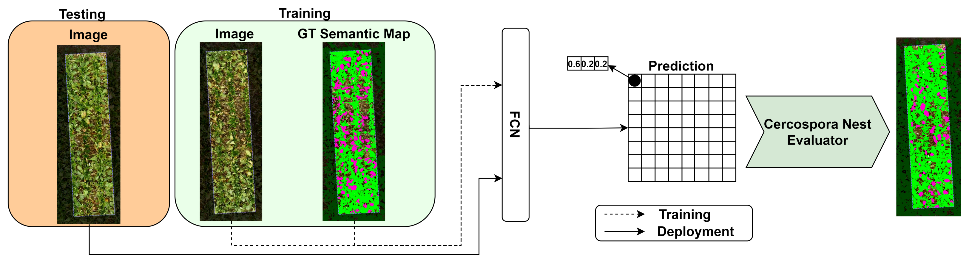
3. Classification System for Plant Disease Detection

The primary objective of our work was to detect and quantify CLS in sugar beet trials robustly. With our approach, we can provide breeders with information about the disease severity within their fields on a plot basis. We developed a semantic segmentation pipeline that explicitly distinguishes between the classes CLS, healthy sugar beet, and background, i.e., mostly soil.

Our approach was designed to process three-channel RGB images as the input. The output is a pixel-wise pseudo probability distribution over the class labels mentioned above. We picked per pixel the class label with the highest probability and obtained the final class map with the same resolution as the original image.

Our fully convolutional network was based on the architecture that we proposed in our previous work [18] for semantic segmentation and stem detection. Fully convolutional DenseNets, proposed by Jégou et al. [37], inspired the architectural design for our semantic segmentation approach. Their FC-DenseNet architecture was based on DenseNet, which was introduced by Huang et al. [38].

In general, the architecture of our approach is structured into three different parts: pre-processing, image encoding, and feature decoding. Figure 2 illustrates our FCN approach’s general processing pipeline.

3.1. Preprocessing

Our pipeline begins with an automatic preprocessing step of the network’s input. By aligning the distributions of the training and test data, preprocessing the network’s inputs can improve the classification system’s generalization capabilities. It includes transforming the pixel values, typically ranging between $[0,255]$, into the range of $[0,1]$. This transformation is carried out by subtracting each channel’s mean value and dividing this result by each channel’s standard deviation, i.e., a standardization. Afterward, we zero centered the data to $[-0.5,0.5]$.

3.2. Encoder Structure

The preprocessing step is followed by the encoder, which serves as a feature extractor. Our encoder incorporates five fully convolutional dense building blocks for the densely compressed feature extraction of the network’s input. The basic building block in our FCN’s encoder structure follows the idea of the so-called fully convolutional DenseNet (FC-DenseNet) [37]. It combines the recently proposed densely connected CNNs, which are organized as dense blocks [38], with fully convolutional networks (FCN) [39]. The dense connectivity pattern iteratively concatenates all computed feature maps of subsequent convolutional layers in a feed-forward fashion. These dense connections encourage deeper layers to reuse features that were produced by earlier layers. Additionally, it supports the gradient flow in the backward pass and thus a stable training. After passing the RGB input images through the encoder, they are transformed into a more compressed and high-level representation.

3.3. Decoder Structure

Our decoder structure closely follows the previously described encoder. It is used to bring the compressed feature representation of the input volume back to the original resolution. The decoder achieves this by applying learned transposed convolutions to the dense feature representations until the resolution of the original input image is matched. Additionally, we included skip connections between the encoder and decoder, supporting the restoration of the spatial information, which might get lost within the encoder structure. Each pixel contains, within the original-sized output, assignment probabilities of belonging to each possible class after passing through a final softmax layer.

The resulting output is a semantic map in which the pixel-wise final class labels are stated. The final class label assignment is based on choosing the class having the highest assignment probability.

4. Experimental Evaluation

Our experiments were designed to show our method’s capabilities and support our key claims, which were: (i) our approach can detect CLS with high performance when testing under similar field conditions; (ii) our approach generalizes well to changing conditions; (iii) the classification system’s results of our proposed approach correlate well to field experts’ scoring results. Hence, our classification system can robustly classify CLS and is a valuable tool for the evaluation of genotypes in the breeding process or plant varieties in registration or recommendation trials.

4.1. Experimental Setup

Data assessment was performed in official breeding trials all over Germany. At each experimental site, several sugar beet genotypes are cultivated in a randomized plot design, and each plot consists of 3 rows. The data set was from different time points during the vegetation period, and all characteristic phases of CLS infection from healthy to severe were observed. Reference ground truth data for calibration in Experiment 3 were assessed at one trial side in North-Rhine-Westphalia in September. We show an illustration for one of these plots in Figure 1.

In the trials that we analyzed, the infection by Cercospora beticola was not inoculated, but appeared naturally as the plants grew on fields that are prone to this disease.

The manually labeled portion of the datasets consisted of around 80 sugar beet plots. Various visual appearances of infested and healthy sugar beets, changing light conditions, and environmental conditions were present in the datasets. In total, we recorded and manually labeled the datasets among 16 different locations across Germany.

The images were captured by a Phase One IMX 100 megapixel RGB camera attached to a M600 drone manufactured by DJI. This drone has a payload of 6 kg, so it can easily carry the employed camera.

4.2. Parameters

In our experiments, we trained all networks from scratch using previously generated random image patches with a resolution of $320\times 320$ pixels. During training, we considered $K=2$ pairs $(\mathit{m}\widehat{\mathit{y}},\mathit{m}\mathit{y})$ within each batch. Hereby, $\mathit{m}\widehat{\mathit{y}}$ denotes the predicted semantic map, and $\mathit{m}\mathit{y}$ represents the ground truth labels of the image patches, each represented as a vector. Moreover, we applied randomized augmentations to the training image patches to reduce overfitting of the model.

We used a positive weighted cross-entropy loss function to evaluate the difference between the predicted semantic map and the ground truth semantic map. It is calculated as follows:

$$\begin{array}{c}\begin{array}{cc}{\mathcal{L}}_{\mathrm{CE}}\left(y,\widehat{y}\right)\hfill & =\frac{1}{K}\sum _{k=1}^K\sum _{c=1}^{C=3}\left(1-y_c^k\right)·{\widehat{y}}_c^k+\hfill \\ & \left(1+\left({\omega }_c-1\right)·y_c^k\right)·\hfill \\ & \left(log\left(1+{exp}^{-\mid {\widehat{y}}_c^k\mid }\right)+max\left(-{\widehat{y}}_c^k,0\right)\right),\hfill \end{array}\hfill \end{array}$$

where k represents the current image. Additionally, ${\omega }_c$ denotes the weight of class c; ${\widehat{y}}_c^k$ is the predicted semantic map of image k; and $y_c^k$ represents the provided ground truth semantic map of image k. The weights ${\omega }_c$ depend on the occurrence of each class within the training dataset. We assigned 10, 1, and 1 for the respective classes of CLS, healthy vegetation, and background.

We trained our network through 150 epochs and chose $0.005$ as the initial learning rate. We also introduced a learning rate schedule that improved convergence by decreasing the learning rate after a predefined number of epochs. To improve generalization, we used a dropout rate of $0.33$. As our parameter initialization values, we sampled a random set from a uniform distribution with a lower boundary of $0.05$ and an upper boundary of $0.15$. For gradient-based parameter optimization, we used the Adam algorithm by Kingma et al. [40].

4.3. Performance under Similar Field Conditions

In this first experiment, we evaluated our network’s performance results in detecting CLS within every single plot when testing on data captured in the same agricultural field (but in a different area) where the training data were acquired. In addition, we ensured that the used images were captured under similar light and environmental field conditions. Therefore, we used a dataset that contained 38 plot images recorded in the same sugar beet field within one flight. Exemplary images used within this experimental setup are visualized in Figure 3.

We captured these plot images in the field shown in Figure 1. We split the total amount of 38 RGB images into a training and test dataset with a ratio of $50/50$. Thus, we used 19 plot images for training and 19 pictures solely for testing. As previously mentioned, these performance results can be seen as the upper boundary of the experimental setup explained in Section 4.4, as the training and test data came from a rather similar distribution.

In

Table 1. Visualization of the resulting output of the CLS classification. In the first image from the left, we show the original RGB image. In the rightmost image, we visualize the agreement between the pixel-wise labels of the predicted semantic map (third image from the left) and the pixel-wise labels of the ground truth semantic map (second image from the left) using green pixels (agreement) and red pixels (disagreement). Within the semantic maps, we represent the class CLS as red pixels and the class healthy vegetation as green pixels, and all remaining pixels belong to the class background.

Image Patch	Ground Truth	Prediction	Agreement

, we show exemplary output results of our first experimental setup.

Visually, the performance results under similar conditions led to rather good classification results for the class CLS. We came to this view because, as depicted in Table 1, almost all pixels labeled as CLS within the ground truth were correctly predicted by our network as CLS. Hence, the class CLS’s recall value should be high, which was confirmed by a corresponding value of around $85\%$. The performance results of this experimental setup are summarized in

Table 2. Class-wise evaluation of the pixel-wise classification performance of the classes CLS, healthy vegetation, and background. Classification performance for the first experiment under similar field conditions. We evaluated using the IoU, precision, recall, and F1 scores. All presented results are given in %.

Class-Wise Evaluation under Similar Field Conditions
Classes	IoU	Precision	Recall	F1 Score
CLS	31.39	33.27	84.75	47.78
healthy vegetation	73.44	96.32	75.57	84.69
background	90.00	98.43	91.31	94.74
⌀	64.94	76.00	83.87	75.74

. As can be seen in Table 2, the high recall of $85\%$ contrasts with a rather low precision value of around $33\%$. The reason for the low precision value is also visible in Table 1. Our network predicted the class CLS at more pixel locations within the prediction map than were actually labeled as infected in the ground truth. This is especially recognizable in the upper left corner of the test image in the last row of Table 1, where there are much more CLS-labeled pixels in the predicted semantic map in comparison to the ground truth. In the table, it can be seen that the network correctly predicted leaves that were totally damaged, while it tended to overestimate the spread of the infection in leaves that were only partially affected.

In general, the classification of the class background worked highly satisfactorily, recognizable by very the high-performance results in terms of the intersection over union (IoU), precision, and recall. This observation was confirmed both visually and with numbers, such as an IoU of $90\%$, a precision of around $98\%$, and a recall of around $91\%$. In contrast, the class vegetation only showed high-performance results when facing a precision value of $96\%$. That means almost all pixels predicted as vegetation were labeled within the ground truth as vegetation as well. The IoU value of $73\%$, as well as the recall of around $76\%$ were not as good as the corresponding values for the class background, but this was because most pixels wrongly classified as CLS actually belonged to the vegetation class. The wrongly assigned pixels resulted in a low IoU and recall for the vegetation class.

4.4. Performance under Changing Conditions

Within the second experiment, we examined whether our trained classification model achieved a good performance in detecting the CLS disease, which developed on a subset of the plants, even under changing light and environmental conditions during the capturing process. Hence, we aimed to reach a certain generalization capability of our network to different environment variables. The symptom development of CLS is dynamic. Early symptoms differ in size, color, and shape from a late symptoms [41]. Furthermore, different leaf stages (young or old leaves) can be diseased preferably. This poses a big challenge to the classifier by itself. Moreover, different lightning and points of view in the analyzed images made the classification problem even harder. Therefore, we used image data captured at 16 different locations at different times of the day to ensure a broad spectrum of environmental conditions during the capturing process. Figure 4 in comparison to Figure 3 shows one exemplary plot image, which illustrates that in differently located sugar beet fields, the light and environmental conditions, as well as plant appearances and soil conditions could vary dramatically.

Within this experiment, we used 38 plot images, captured at 15 different locations, for training. We then used 38 plots from another location as the testing dataset. By this data partitioning, we aimed at providing enough training information from different perspectives to the network. We, therefore, expected our approach to generalize well enough to correctly classify the test set acquired under unseen conditions.

In

Table 3. Visualization of the resulting output of the CLS classification. In the first image from the left, we show the original RGB image. In the rightmost image, we visualize the agreement between the pixel-wise labels of the predicted semantic map (third image from the left) and the pixel-wise labels of the ground truth semantic map (second image from the left) using green pixels (agreement) and red pixels (disagreement). Within the semantic maps, we represent the class CLS as red pixels and the class healthy vegetation as green pixels, and all remaining pixels belong to the class background.

Image Patch	Ground Truth	Prediction	Agreement

, we show exemplary output results of our second experimental setup.

The visual evaluation of these results showed that, generally, the classification of CLS-labeled pixels was characterized by a good performance regarding the recall. This was in line with the previous experiment, and we saw a certain generalization. As is visible in the top and bottom row of Table 3, almost all occurring CLS-labeled pixels were classified correctly by our network. Only a few false-negative pixels classified as CLS were recognizable. This generally happened only when the network predicted a small part of the damaged leaf instead of the entire infected surface. In the bottom row of Table 3, the network extended its CLS prediction to the background in some parts, especially in the upper left corner of the image. We imputed this to very similar colors of the soil and rotten leaves.

We can confirm this observation by considering the performance results regarding the IoU, precision, recall, and F1 score [42]. We show these results in

Table 4. Class-wise evaluation of the pixel-wise classification performance of the classes CLS, healthy vegetation, and background. Classification performance for the second experiment under changing field conditions. We evaluated using the IoU, precision, recall and F1 scores. All presented results are given in %.

Class-Wise Evaluation under Changing Field Conditions
Classes	IoU	Precision	Recall	F1 Score
CLS	28.60	33.37	66.69	44.48
healthy vegetation	78.99	92.58	84.33	88.26
background	88.50	98.47	89.73	93.90
⌀	65.36	74.81	80.25	75.55

. Concerning the class CLS, the pixels labeled with this specific class were recognized with a recall of about $67\%$. However, the precision was $33\%$, as in the first experiment. This was in line with our observations in Table 3, in which the predicted semantic map included most CLS-labeled pixels of the ground truth semantic map, but extended this prediction to certain soil and vegetation areas.

The classes healthy vegetation and background showed high-performance results with respect to the IoU, precision, and recall. Especially the class background with an IoU of around $89\%$, a precision of around $98\%$, and a recall value of around $90\%$ was classified well. Furthermore, the class vegetation showed satisfying results with an IoU of $79\%$, a precision of around $93\%$, and a recall of $84\%$.

In general, the achieved recall for the class CLS of around $67\%$ was acceptable, but compared to the remaining two classes, the performance results were less precise. Considering the fact that the test images were captured under light conditions, as well as plant and soil appearances never seen by the network, the resulting recall value of the class CLS was quite good. This was especially true when considering the upper boundary, which we determined in our first experimental setup in Section 4.3. Regarding the precision, the performance results of the generalized network were identical to the upper bound value.

Regarding the classes healthy vegetation and background, both networks’ resulting performances did not strongly differ from one another. That means the generalization of soil and vegetation did not seem to be challenging for our approach.

In conclusion, the performance results of the first two experimental setups, the classification of CLS, led to quite satisfying performance results regarding the recall. When considering the precision instead, the classification did not perform as well. In this regard, it should be noted that the detection of CLS is a difficult problem also for an expert human operator. Especially in early disease stages, symptoms are hard to detect accurately as they result in an appearance that is only slightly different from a healthy leaf. We, therefore, performed a third experiment, presented in the next section, to show that the performance of our approach led to a quantification of the spread of CLS, which was comparable to the one obtained by experts examining the plants visually on site.

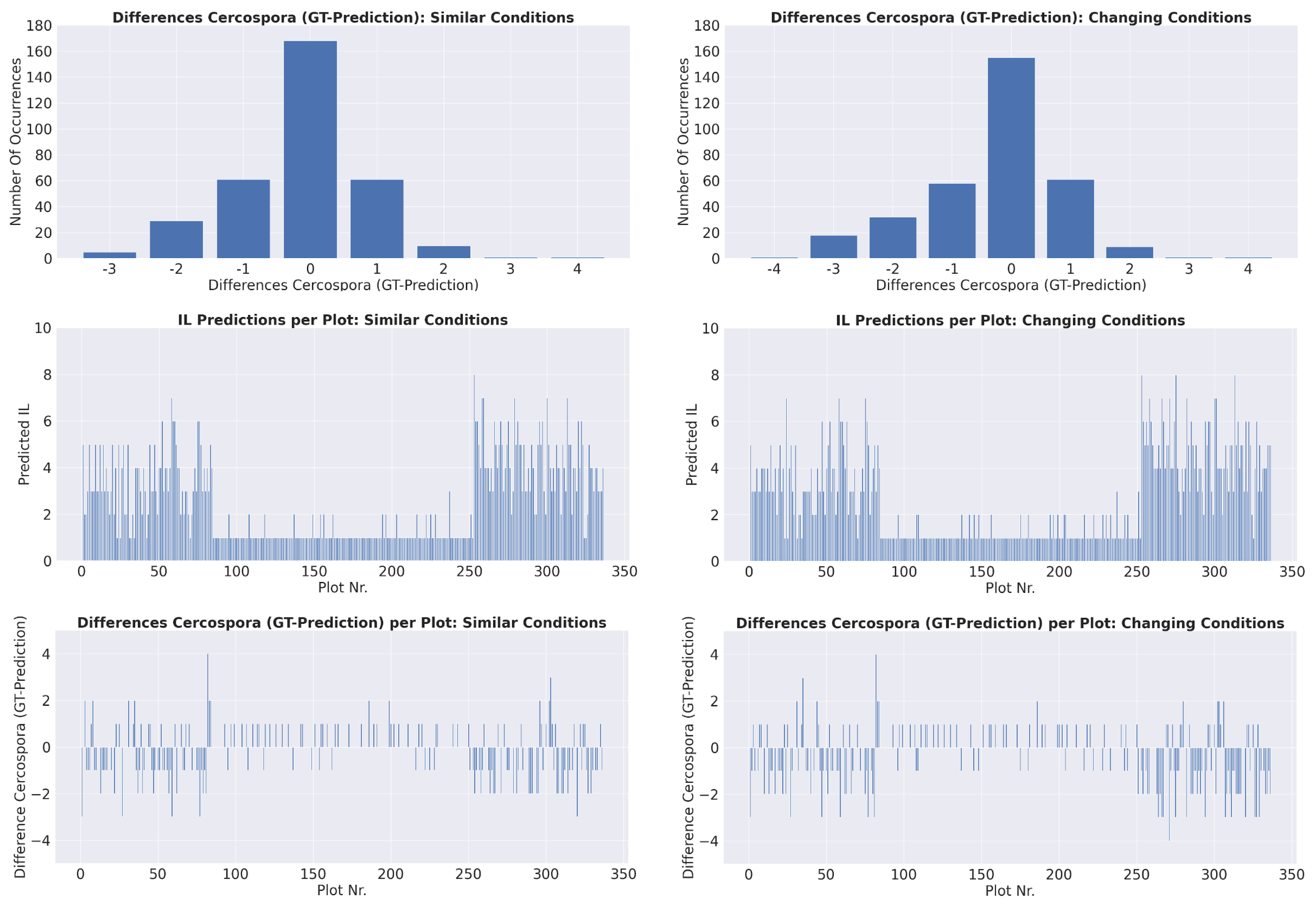
4.5. Comparison of the Estimated Level of Infection and the Experts’ Scoring Results

To correlate our network output with the experts’ scoring results in the third experiment, we needed to derive a value that was comparable to the scoring values used by them. We further refer to these derived values as infection levels. They describe the severity of infection by CLS on sugar beet plants within the individual plots via an ordinal rating scale. For this evaluation, an expert went into the field to determine the infection level of the plots. Therefore, the determination of the infection level is a time-consuming and expensive task for farmers and breeders. Since the fields were organized into plots, each of these single plots was assigned a score. This single number represented the infection level of CLS on the sugar beet plants within this certain plot. The infection level was a number in the range between 1 and 9. No infection or a very small infection was set as 1; 5 meant a mediocre infection; and 9 represented very heavily infested plants [43].

The ground truth data were provided by the breeding company Strube Research and were based on the experts’ scoring of the infection level of CLS for 336 plots. The trial was comprised of 84 entries, which were laid out over 2 strips. The entries of the trial were replicated 4 times. Two of those replicates were treated with fungicide (Strips 3-4 and 5-6), and the other two were not treated with fungicide (Strips 1-2 and 7-8). We expected high infection levels in the strips where no fungicide was applied and lower scores for the other strips. The eight strips with 42 entries each are numbered in Figure 1. The data used in this experiment were collected by two experts with 12 and 25 years of experience, respectively. They used an evaluation scheme developed by Strube and used for 20 years to ensure a consistent interpretation of the symptoms.

In order to compare the classification system’s results, we first needed to derive comparable values. Therefore, we analyzed the classified image pixels’ distribution within the predicted semantic map, which we obtained after applying the previously trained classifier. We focused on the resulting semantic map we obtained using the classifier trained under similar conditions (Section 4.3) and the one obtained under changing conditions (Section 4.4).

In the infection level estimation process, we only considered the pixels that were predicted as CLS, since healthy vegetation and background were not relevant for this task. To convert the number of pixels predicted as CLS into the infection level score, we first defined the lower and upper boundaries. For the first boundary, we calculated the average occurrence of CLS pixels within all plots that were rated as Infection Level 1 in the ground truth defined by the experts. We then defined as 1 the infection level off all plots with a number of pixels classified as infected that was lower than or equal to the calculated average. We used this averaging instead of simply assigning the lowest value to the first score, which was more in line with the expert evaluation. The same procedure was applied by us to find the amount of CLS pixels relative to Infection Level 8, taking into consideration the most infected plots instead. We here used the score of 8 instead of the maximum possible infection level of 9 since the ground truth data contained only infection levels in the range between 1 and 8. This allowed us to actually define the plots with the lowest-rated infection level as 1 instead of interpolating them to a higher score. Based on our predicted infection levels’ lower and upper boundary, we performed linear interpolation to find the occurrence frequencies of CLS corresponding to the different scores. By finding the score corresponding to an occurrence frequency that was closest to the one of a given plot, we could assign this score to the plot. This resulted in an estimated infection level for every single plot. Now, we could compare these predictions with the corresponding expert’s ground truth scoring values.

Figure 5 contains the results obtained from the images of both the classifier trained under similar, as well as the one trained under changing conditions. In the leftmost image in the upper row, we see a histogram showing the difference between the ground truth value and the corresponding predicted infection level. Here, the estimated infection levels were based on the semantic maps predicted using the classifier, which was trained under similar field conditions (Section 4.3). Underneath, in the bottom row’s leftmost figure, we show the histogram of the differences between the ground truth and the prediction based on the semantic maps obtained using the classifier trained under changing field conditions (Section 4.4). In the upper row’s central figure, we present the difference between the ground truth and the predicted infection level for each plot, based on the output of the classifier trained under similar conditions. Below this plot, we show the counterpart based on the classifier trained under changing field conditions. We visualize the predicted infection level of the plots based on the two classifiers on the right-hand side.

As clearly visible within both histograms, the most occurring difference between the ground truth and the prediction was 0, equaling 29.8%. In addition, regarding the differences $\pm 1$ often occurring within the histograms, they could be observed in 51.5% of the plots. This led to the insight that the estimation of the infection levels based on our networks’ semantic maps correlated well to the experts’ scoring values. We came to this conclusion because in practice, the infection level determination is highly subjective and depends on each expert [44,45]. This led to the fact that, sometimes, an expert evaluates an area with a different scoring value than another expert would have done. Therefore, a deviation of $\pm 1$ of the experts’ scores seemed reasonable. The resulting accuracy with a $\pm 1$ tolerance was 81.2%.

The plots on the right-hand side correlate to the ground truth data distribution we explained at the beginning of this section. Both classifiers predicted rather high infection levels for the first two rows of the breeder’s field, small scores for Rows 3 to 6, and high CLS infection in Rows 7 and 8.

5. Conclusions

In this paper, we showed that we could determine Cercospora leaf spot (CLS) with a high recall, but a rather low precision, in the presence of mostly healthy sugar beet plants when using data that were captured under similar field conditions as the testing data. Additionally, we could classify healthy vegetation and background with F1 scores higher than $80\%$. Moreover, we demonstrated that we achieved a certain generalization regarding various light and environmental conditions during the data acquisition while classifying CLS’s occurrence, underlined by a recall of around $66\%$ for the class CLS. This generalization was also observable when considering the F1 score values of the classes healthy vegetation and background, which were higher than $88\%$. Considering the fact that this work was a proof-of-concept, the resulting performance of CLS detection was acceptable and showed that this approach is worth being studied further. Most of the false negatives were classified as healthy vegetation, which in our opinion were derived mostly from the difficulty of visually determining the CLS symptoms, which made it almost impossible to label the data with very high accuracy. Here also the resolution of the images played a big role. We showed that this approach is already valuable by verifying that estimated infection levels derived from the semantic map predicted by our network correlated well with the experts’ scoring values. Still, there is room for improvement by using a bigger dataset, and experts could be involved in the labeling process to obtain a better ground truth. Furthermore, an increased resolution of the RGB images would most likely improve the result, especially regarding the detection of early symptoms.

References

1. Savary, S.; Willocquet, L. Modeling the Impact of Crop Diseases on Global Food Security. Annu. Rev. Phytopathol. 2020, 58, 313–341. [Google Scholar] [CrossRef]
2. Mahlein, A.K.; Kuska, M.T.; Thomas, S.; Wahabzada, M.; Behmann, J.; Rascher, U.; Kersting, K. Quantitative and qualitative phenotyping of disease resistance of crops by hyperspectral sensors: Seamless interlocking of phytopathology, sensors, and machine learning is needed! Curr. Opin. Plant Biol. 2019, 50, 156–162. [Google Scholar] [CrossRef] [PubMed]
3. Furbank, R.T.; Tester, M. Phenomics—Technologies to relieve the phenotyping bottleneck. Trends Plant Sci. 2011, 16, 635–644. [Google Scholar] [CrossRef] [PubMed]
4. Bonatti, R.; Wang, W.; Ho, C.; Ahuja, A.; Gschwindt, M.; Camci, E.; Kayacan, E.; Choudhury, S.; Scherer, S. Autonomous aerial cinematography in unstructured environments with learned artistic decision-making. J. Field Robot. 2020, 37, 606–641. [Google Scholar] [CrossRef] [Green Version]
5. Patrikar, J.; Moon, B.; Scherer, S. Wind and the City: Utilizing UAV-Based In-Situ Measurements for Estimating Urban Wind Fields. In Proceedings of the (IROS) IEEE/RSJ International Conference on Intelligent Robots and Systems, Las Vegas, NV, USA, 25–29 October 2020. [Google Scholar]
6. Pavan Kumar, B.N.; Balasubramanyam, A.; Patil, A.K.; Chethana, B.; Chai, Y.H. GazeGuide: An Eye-Gaze-Guided Active Immersive UAV Camera. Appl. Sci. 2020, 10, 1668. [Google Scholar] [CrossRef] [Green Version]
7. Radoglou-Grammatikis, P.; Sarigiannidis, P.; Lagkas, T.; Moscholios, I. A compilation of UAV applications for precision agriculture. Comput. Netw. 2020, 172, 107148. [Google Scholar] [CrossRef]
8. Christiansen, M.P.; Laursen, M.S.; Jørgensen, R.N.; Skovsen, S.; Gislum, R. Designing and Testing a UAV Mapping System for Agricultural Field Surveying. Sensors 2017, 17, 2703. [Google Scholar] [CrossRef] [Green Version]
9. Weiland, J.; Koch, G. Sugarbeet leaf spot disease (Cercospora beticola Sacc.) dagger. Mol. Plant Pathol. 2004, 5, 157–166. [Google Scholar] [CrossRef]
10. Imbusch, F.; Liebe, S.; Erven, T.; Varrelmann, M. Dynamics of cercospora leaf spot disease determined by aerial spore dispersal in artificially inoculated sugar beet fields. Plant Pathol. 2021, 70, 853–861. [Google Scholar] [CrossRef]
11. Jay, S.; Comar, A.; Benicio, R.; Beauvois, J.; Dutartre, D.; Daubige, G.; Li, W.; Labrosse, J.; Thomas, S.; Henry, N.; et al. Scoring Cercospora Leaf Spot on Sugar Beet: Comparison of UGV and UAV Phenotyping Systems. Plant Phenomics 2020, 1–18. [Google Scholar] [CrossRef]
12. Treml, M.; Arjona-Medina, J.; Unterthiner, T.; Durgesh, R.; Friedmann, F.; Schuberth, P.; Mayr, A.; Heusel, M.; Hofmarcher, M.; Widrich, M.; et al. Speeding up semantic segmentation for autonomous driving. In Proceedings of the MLITS, NIPS Workshop, Barcelona, Spain, 9 December 2016; Volume 2, p. 7. [Google Scholar]
13. Quan, T.M.; Hildebrand, D.G.; Jeong, W.K. Fusionnet: A deep fully residual convolutional neural network for image segmentation in connectomics. arXiv 2016, arXiv:1612.05360. [Google Scholar]
14. Ronneberger, O.; Fischer, P.; Brox, T. U-net: Convolutional networks for biomedical image segmentation. In Proceedings of the International Conference on Medical Image Computing and Computer-Assisted Intervention, Munich, Germany, 5–9 October 2015; pp. 234–241. [Google Scholar]
15. Athar, A.; Mahadevan, S.; Ošep, A.; Leal-Taixé, L.; Leibe, B. STEm-Seg: Spatio-temporal Embeddings for Instance Segmentation in Videos. In Proceedings of the European Conference on Computer Vision (ECCV), Glasgow, UK, 23–28 August 2020. [Google Scholar]
16. Engelmann, F.; Bokeloh, M.; Fathi, A.; Leibe, B.; Nießner, M. 3D-MPA: Multi Proposal Aggregation for 3D Semantic Instance Segmentation. In Proceedings of the IEEE Conference on Computer Vision and Pattern Recognition (CVPR), Seattle, WA, USA, 13–19 June 2020. [Google Scholar]
17. Weber, M.; Luiten, J.; Leibe, B. Single-Shot Panoptic Segmentation. arXiv 2019, arXiv:1911.00764. [Google Scholar]
18. Lottes, P.; Behley, J.; Chebrolu, N.; Milioto, A.; Stachniss, C. Joint Stem Detection and Crop-Weed Classification for Plant-specific Treatment in Precision Farming. In Proceedings of the IEEE/RSJ International Conference on Intelligent Robots and Systems (IROS), Madrid, Spain, 1–5 October 2018. [Google Scholar]
19. Lottes, P.; Behley, J.; Milioto, A.; Stachniss, C. Fully Convolutional Networks with Sequential Information for Robust Crop and Weed Detection in Precision Farming. IEEE Robot. Autom. Lett. RA-L 2018, 3, 3097–3104. [Google Scholar] [CrossRef] [Green Version]
20. Milioto, A.; Lottes, P.; Stachniss, C. Real-time Semantic Segmentation of Crop and Weed for Precision Agriculture Robots Leveraging Background Knowledge in CNNs. In Proceedings of the IEEE International Conference on Robotics & Automation (ICRA), Brisbane, Australia, 21–25 May 2018. [Google Scholar]
21. Mortensen, A.; Dyrmann, M.; Karstoft, H.; Jörgensen, R.N.; Gislum, R. Semantic Segmentation of Mixed Crops using Deep Convolutional Neural Network. In Proceedings of the International Conference of Agricultural Engineering (CIGR), Aarhus, Denmark, 26–29 June 2016. [Google Scholar]
22. Zhang, S.; Wang, H.; Huang, W.; You, Z. Plant diseased leaf segmentation and recognition by fusion of superpixel, K-means and PHOG. Optik 2018, 157, 866–872. [Google Scholar] [CrossRef]
23. Mahlein, A.K.; Rumpf, T.; Welke, P.; Dehne, H.W.; Plümer, L.; Steiner, U.; Oerke, E.C. Development of spectral indices for detecting and identifying plant diseases. Remote Sens. Environ. 2013, 128, 21–30. [Google Scholar] [CrossRef]
24. Bhange, M.; Hingoliwala, H. Smart farming: Pomegranate disease detection using image processing. Procedia Comput. Sci. 2015, 58, 280–288. [Google Scholar] [CrossRef] [Green Version]
25. Padol, P.B.; Yadav, A.A. SVM classifier based grape leaf disease detection. In Proceedings of the 2016 Conference on Advances in Signal Processing (CASP), Pune, India, 9–11 June 2016. [Google Scholar]
26. Kaur, P.; Pannu, H.; Malhi, A. Plant disease recognition using fractional-order Zernike moments and SVM classifier. Neural Comput. Appl. 2019, 31, 8749–8768. [Google Scholar] [CrossRef]
27. Singh, V.; Misra, A.K. Detection of plant leaf diseases using image segmentation and soft computing techniques. Inf. Process. Agric. 2017, 4, 41–49. [Google Scholar] [CrossRef] [Green Version]
28. Zhou, R.; Kaneko, S.; Tanaka, F.; Kayamori, M.; Shimizu, M. Image-based field monitoring of Cercospora leaf spot in sugar beet by robust template matching and pattern recognition. Comput. Electron. Agric. 2015, 116, 65–79. [Google Scholar] [CrossRef]
29. Amara, J.; Bouaziz, B.; Algergawy, A. A Deep Learning-Based Approach for Banana Leaf Diseases Classification. Datenbanksysteme für Business, Technologie und Web (BTW 2017) Workshopband 2017. pp. 79–88. Available online: https://www.semanticscholar.org/paper/A-Deep-Learning-based-Approach-for-Banana-Leaf-Amara-Bouaziz/9fcecc67da35c6af6defd6825875a49954f195e9 (accessed on 21 March 2021).
30. Ferentinos, K.P. Deep learning models for plant disease detection and diagnosis. Comput. Electron. Agric. 2018, 145, 311–318. [Google Scholar] [CrossRef]
31. Mohanty, S.P.; Hughes, D.P.; Salathé, M. Using deep learning for image-based plant disease detection. Front. Plant Sci. 2016, 7, 1419. [Google Scholar] [CrossRef] [PubMed] [Green Version]
32. Ozguven, M.M.; Adem, K. Automatic detection and classification of leaf spot disease in sugar beet using deep learning algorithms. Phys. A Stat. Mech. Its Appl. 2019, 535, 122537. [Google Scholar] [CrossRef]
33. Sladojevic, S.; Arsenovic, M.; Anderla, A.; Culibrk, D.; Stefanovic, D. Deep Neural Networks Based Recognition of Plant Diseases by Leaf Image Classification. Comput. Intell. Neurosci. 2016, 1–11. [Google Scholar] [CrossRef] [PubMed] [Green Version]
34. Wang, G.; Sun, Y.; Wang, J. Automatic image-based plant disease severity estimation using deep learning. Comput. Intell. Neurosci. 2017, 1–8. [Google Scholar] [CrossRef] [PubMed] [Green Version]
35. Lin, K.; Gong, L.; Huang, Y.; Liu, C.; Pan, J. Deep learning-based segmentation and quantification of cucumber Powdery Mildew using convolutional neural network. Front. Plant Sci. 2019, 10, 155. [Google Scholar] [CrossRef] [Green Version]
36. Yi, J.; Krusenbaum, L.; Unger, P.; Hüging, H.; Seidel, S.; Schaaf, G.; Gall, J. Deep Learning for Non-Invasive Diagnosis of Nutrient Deficiencies in Sugar Beet Using RGB Images. Sensors 2020, 20, 5893. [Google Scholar] [CrossRef]
37. Jégou, S.; Drozdzal, M.; Vazquez, D.; Romero, A.; Bengio, Y. The one hundred layers tiramisu: Fully convolutional densenets for semantic segmentation. In Proceedings of the IEEE Conference on Computer Vision and Pattern Recognition Workshops, Honolulu, HI, USA, 21–26 July 2017; pp. 11–19. [Google Scholar]
38. Huang, G.; Liu, Z.; Maaten, L.; Weinberger, K.Q. Densely Connected Convolutional Networks. In Proceedings of the IEEE Conference on Computer Vision and Pattern Recognition (CVPR), Honolulu, HI, USA, 21–26 July 2017. [Google Scholar]
39. Long, J.; Shelhamer, E.; Darrell, T. Fully Convolutional Networks for Semantic Segmentation. In Proceedings of the IEEE Conference on Computer Vision and Pattern Recognition (CVPR), Boston, MA, USA, 7–12 June 2015. [Google Scholar]
40. Kingma, D.P.; Ba, J. Adam: A method for stochastic optimization. arXiv 2014, arXiv:1412.6980. [Google Scholar]
41. Mahlein, A.K.; Steiner, U.; Hillnhütter, C.; Dehne, H.W.; Oerke, E.C. Hyperspectral imaging for small-scale analysis of symptoms caused by different sugar beet disease. Plant Methods 2012, 8, 1–13. [Google Scholar] [CrossRef] [Green Version]
42. Sasaki, Y. The Truth of the F-Measure. Teach Tutor Mater 2007. Available online: https://www.cs.odu.edu/~mukka/cs795sum09dm/Lecturenotes/Day3/F-measure-YS-26Oct07.pdf (accessed on 21 March 2021).
43. Wilbois, K.P.; Schwab, A.; Fischer, H.; Bachinger, J.; Palme, S.; Peters, H.; Dongus, S. Leitfaden für Praxisversuche. Available online: https://orgprints.org/2830/3/2830-02OE606-fibl-wilbois-2004-leitfaden_praxisversuche.pdf (accessed on 25 May 2020).
44. Nutter, F., Jr.; Esker, P.; Netto, R.; Savary, S.; Cooke, B. Disease Assessment Concepts and the Advancements Made in Improving the Accuracy and Precision of Plant Disease Data. Eur. J. Plant Pathol. 2007, 115, 95–103. [Google Scholar] [CrossRef]
45. Bock, C.; Barbedo, J.; Del Ponte, E.; Bohnenkamp, D.; Mahlein, A.K. From visual estimates to fully automated sensor-based measurements of plant disease severity: Status and challenges for improving accuracy. Phytopathol. Res. 2020, 2, 1–30. [Google Scholar] [CrossRef] [Green Version]
Figure 1. We aimed at predicting the occurrence of Cercospora leaf spot (CLS) for the entire field trial. We first separated the RGB orthomosaic into small plots that corresponded to the breeder’s plot structure for variety testing. These plots were divided into eight strips, which are numbered in red. For each plot, we performed a pixel-wise classification into the classes CLS (pink), healthy vegetation (green), and background (no color). Finally, we illustrate the plot-based infection level for the entire field in semantic maps, where a red plot refers to high infection and blue refers to no infection. We flew a DJI M600 equipped with a Phase One IMX 100 megapixel RGB camera.
Drones 05 00034 g001
Figure 2. Overview of the approach, developed with precision farming applications in mind. It briefly illustrates the FCN approach for the classification of CLS based on RGB images only.
Drones 05 00034 g002
Figure 3. A single plots’ RGB and corresponding ground truth information. The pixels labeled as Cercospora leaf spot (CLS) are in pink, whereas healthy vegetation is represented by green pixels. Note that this is a single plot from the field illustrated in Figure 1, but rotated 90 ° .
Drones 05 00034 g003
Figure 4. The images show an exemplary plot at another location in comparison to the breeder’s field visualized in Figure 1 and Table 1. In different sugar beet field locations, the conditions can strongly differ from one another.
Drones 05 00034 g004
Figure 5. Results of the infection level (IL) determination of CLS based on the predicted semantic maps. The upper line contains the results based on the semantic maps we obtained using the classifier trained under similar conditions, whereas the lower line consists of the results based on using the classifier trained under changing conditions.
Drones 05 00034 g005