Article

An Approach for Route Optimization in Applications of Precision Agriculture Using UAVs

by
Kshitij Srivastava
1,
Prem Chandra Pandey
2,* and
Jyoti K. Sharma
2
1
Department of Electrical Engineering, Shiv Nadar University, Greater Noida 201314, India
2
Center for Environmental Sciences & Engineering, Shiv Nadar University, Greater Noida 201314, India
*
Author to whom correspondence should be addressed.
Drones 2020, 4(3), 58; https://doi.org/10.3390/drones4030058
Submission received: 23 July 2020 / Revised: 14 September 2020 / Accepted: 16 September 2020 / Published: 18 September 2020
(This article belongs to the Special Issue Feature Papers of Drones)

Abstract

:
This research paper focuses on providing an algorithm by which (Unmanned Aerial Vehicles) UAVs can be used to provide optimal routes for agricultural applications such as, fertilizers and pesticide spray, in crop fields. To utilize a minimum amount of inputs and complete the task without a revisit, one needs to employ optimized routes and optimal points of delivering the inputs required in precision agriculture (PA). First, stressed regions are identified using VegNet (Vegetative Network) software. Then, methods are applied for obtaining optimal routes and points for the spraying of inputs with an autonomous UAV for PA. This paper reports a unique and innovative technique to calculate the optimum location of spray points required for a particular stressed region. In this technique, the stressed regions are divided into many circular divisions with its center being a spray point of the stressed region. These circular divisions would ensure a more effective dispersion of the spray. Then an optimal path is found out which connects all the stressed regions and their spray points. The paper also describes the use of methods and algorithms including travelling salesman problem (TSP)-based route planning and a Voronoi diagram which allows applying precision agriculture techniques.

1. Introduction

One of the main objectives of the United Nations is to have sustainable agriculture which can enhance agricultural productivity to meet the food supply-demand of the increasing population without overexploiting and wasting natural resources [1]. The estimated population is likely to reach nine billion from seven billion by 2050 [2,3]. Significant pressure is expected on agricultural systems to meet the continuously increasing needs of the population, thus escalating human pressures on the environment [3,4,5,6]. Farming is predominantly done on limited space or regions, which are decreasing day by day due to several factors, such as conversion to other land use categories, e.g., farmland to residential, commercial and industrial buildings [7,8]. With the limited land area available, agriculture will have more pressure for increased crop yield to enhance productivity as well as maintain the food quality to cope up with the increasing population’s demands. Several parameters, such as soil moisture, nutrients, such as nitrogen, phosphorus, and potassium [9], water holding capacity, pH and other variables affect crop productivity and thus require continuous monitoring to prevent crop stress. At present, the identification process of stressed regions and preventive measures are performed manually, while the identification of stressed regions is assessed using visual image interpretation using remote sensing and GIS. Moreover, at most of the places, other agricultural applications, such as spraying of pesticides or fertilizers, are performed manually too. This leads to an increased cost and inefficient use of resources, along with wastage of input resources. To maintain quality and enhance the productivity of crops, precision agriculture (PA) has to be adopted by farmers worldwide [10,11].
In recent decades, there has been an increase in the number of techniques and methods employed in agriculture to enhance crop yield and productivity. Pesticides have been used against insects and pests, while fertilizers are used to improve the fertility of the soil by adding major nutrients to enhance crop productivity [12,13]. Moreover, wastage of these agricultural inputs is more common during steps and processes which, overall, impact the expenses in agriculture. In recent years, there has been a gradual shift towards mechanization in agriculture for harvesting, spraying and drip irrigation which has helped to optimize the amount of water used and reduce the wastage.
In the present era, PA is a new concept that has been introduced in agricultural practices to improve agricultural crop yields and help in decision making using advanced geospatial tools and techniques for analysis [14,15]. This is used worldwide nowadays to reduce labor costs, minimize the time duration and assist in the proper management of fertilizers, pesticides and irrigation activities throughout the field in less time [16]. PA also helps in understanding the soil condition and its parameters over time and aims at addressing this soil spatial variability, but for these tasks, spectral images of the land are required [17]. Therefore, a new concept of PA has been introduced to tackle these problems, such as minimizing wastage of agricultural resources inputs and reducing labor time to increase the productivity of the crops [18]. PA is the science of improving crop yields with assisted management using high technology sensors and analysis tools. Advanced multispectral imaging equipment offers innovations in the practical application of PA techniques. This is useful for the valuation of crop stresses, quality of soils and the vegetative cover, as well as for yield estimation [19,20]. The technique also adopts a concept to minimize the wastages and effective management of fertilizers and pesticides for increased crop yields [18]. The everyday practices of agriculture can be observed by UAVs for soil monitoring, early weed detection, disease and pest control, nutrient assessment and fertilizer applications at different spatial scales [21,22,23]. These innovative technologies have been implemented and are in demand for new opportunities in PA by farmers to provide stressed maps, pest infestation maps, soil condition, disease control and yield maps [22,23,24,25].
The above concepts, when implemented in agricultural practices, undoubtedly result in increased agricultural productivity by protecting crops against pests, insects, disease and any stress. Concepts and methods to provide fertilizers at a particular stressed region effectively at appropriate times are also promoted. To realize this, spectral images and thermal images are obtained from the UAVs, which have a high spatial resolution compared to satellite images and are less susceptible to weather conditions [26,27,28]. These are useful for regional mapping and analysis where limited areas are being considered and are in focus.
Spectral and reflectance images from UAVs are incorporated for analysis and assessment in agricultural research and agricultural tasks, as well as decision making [29,30]. In 2008, Nebikera conceptualized the use of the spectral camera on drones for aerial imaging and analysis [31]. Research has demonstrated the usage of these spectral images to assess stressed regions as well as stressed crops based on different soil parameters, water content and plant chlorophyll contents [32]. This was recently demonstrated in our previous study [33] by the development of VegNet (Vegetative Network) software to assess crop stress in a large field by extracting different vegetative indices, such as NDVI (normalized difference vegetation index) [34], NDRE (normalized red difference index) [35], EVI (enhanced vegetation index) [36]. We also incorporated other reflectance indices, such as NDVI, TCARI/OSAVI (transformed chlorophyll absorption in reflectance index/optimized soil adjusted vegetation index), etc. These indices were derived from spectral images and demonstrated that they have a positive correlation to stress indicators (water or nutrients). Both TCARI/OSAVI are very sensitive to chlorophyll content variations which are useful to assess the stress condition of vegetation [37]. The spectral images were employed for the detection of stressed regions in the agricultural fields using the VegNet software application (please refer to [33]). VegNet is an application that was developed with the aim of providing the necessary tools to detect stressed crop locations using spectral images obtained from UAVs, and providing the stressed crops’ condition and location and the area covered by those stressed crops. It has been shown that VegNet has the flexibility to use any combination of reflectance indices, or even thermal indices, for detection of stressed regions.
In the past, UAVs have been used for monitoring agricultural fields with spectral images and then calculating the above-mentioned indices which indicate deficiencies in the field. Even the usage of UAVs in non-agricultural activities, such as monitoring natural resources, such as land, water and rivers [38,39,40], as well as in disaster management [41], has rapidly increased in the past few years. In 2015, Gao [26] demonstrated the use of UAVs for water stress assessment using thermal indices and canopy conductance measurements. Hence, both thermal imagery and spectral imagery obtained from UAVs providing reflectance indices and thermal indices have shown great potential to determine field stress heterogeneity. In 2019, authors developed an application based on a combination of reflectance indices to detect stressed regions in agricultural fields [33].
The soil parameters and use of spectral indicators for water content extraction, plant chlorophyll content and so on have been demonstrated in past research. This was done by extracting different vegetative indices, such as NDVI, NDRE and EVI. While these findings are very helpful in gaining new insights about a farm, these sophisticated vegetative indicators make little sense for a nonprofessional. Even if farmers get to know about the deficiency of nutrients in their crops and the locations of stressed regions, they will still be taking corrective steps manually, which is inefficient and time-consuming, hence optimized use of machinery is suggested. UAVs are also increasingly being used in PA activities, such as administering inputs, apart from monitoring. Thus, UAVs have been employed in supporting PA mapping to effectively manage and provide optimized inputs to agricultural fields, such as water, fertilizers and pesticides, to increase the quality and yield of crops [42,43]. There is still a lot of progress to be made in the way in which corrective measures are applied, such as spraying water, pesticides or fertilizers. Therefore, a system has to be brought to the forefront that addresses the technological gaps and applies the benefits of PA for increasing farm productivity.
Software and information technology (IT) solutions have been developed by researchers on a variety of aspects of precision farming [44,45,46,47]. Most of them have focused on PA by using it primarily for monitoring and analysis purposes and not focused on IT-based mechanization and automation [48]. One of the research papers has tried focusing on providing integrated UAV-based PA using an aerial farm robot that takes care of all agriculture-related activities, such as cropping, planting and fertilizing [49]. It used UAVs that were attached with detachable instruments for this purpose. In this system, they applied fertilizer to all parts of the field equally without any regard for spatial nutrient differences in the land. However, what was needed was for the fertilizer to be applied only on stressed regions and not to all the parts of the field, so there must be a feedback mechanism for nutrient deficient regions and application of fertilizer [48]. Analysis using spectral indices will help in identifying stressed regions and will help in site-specific input applications.
Recent studies have focused on studying the effects of several UAV design parameters on spraying outcomes. Qin et al. illustrated and discussed the influence of spraying parameters, such as the operation height and operation velocity of the UAV, on droplet deposition [50]. Studies also revealed spray factors, such as the speed and distance of UAVs for droplet size, distribution and distribution uniformity [51]. It studied factors, such as the speed and distance of UAVs for droplet size, distribution and distribution uniformity. Most of these papers have focused on the spraying while in motion. In contrast, the present paper suggests spraying fertilizers while the UAV is flying over the spray position. This method of spraying would reduce some of the factors associated with UAVs.
All the past research works have been done on spraying fertilizers and pesticides from UAVs on farms and stressed regions of particular shapes and sizes. This paper will open up the possibilities of working in farms and stressed regions of irregular shapes and sizes which were not addressed earlier. There are a few algorithms that can work on farms of all shapes and sizes, and our algorithm is one among them. One of the early research papers used multiple drones on a full field where the drones were spraying parallel to one another in various rows of the farm [52]. However, the method proposed was not site-specific and no algorithm was proposed for traversing the field. It required the crops to be planted in rows which are to be fed into the system for spraying. In 2013, a unique approach was given where centroidal Voronoi tessellation was used to spread swarm UAVs to cover an infected region. It claimed that the most effective solution, then, is to attack around the infection and contain the situation before fully eradicating the infection. Voronoi divided the region into many parts and drones started spraying from each Voronoi centroid [53]. It could attend to any stressed region, ensure to limit the amount of spraying over healthy plants and avoid overlapping of pesticide spraying. Nevertheless, this method required many UAVs for attending to a single stressed region, making it very resource-intensive. In 2017, another article looked at using UAVs to find stressed regions and then spraying on the stressed patches using a tractor with many spraying nozzles that could be turned on and off depending upon the patches [54]. However, the authors failed to provide an algorithm for spraying on the stressed regions. In 2019, another study looked into site-specific management during the vineyard spraying process. Here, the authors also used UAVs to find stressed regions. They divided the stressed regions into three different zones indicating different levels of canopy vigor. The application map was divided into small and irregular rectangles. The width of the rectangle was decided such that it corresponded to the working width of the sprayer [55]. However, the problem with this approach is that this division of stressed regions is done in the form of a rectangular shape, which is not the most appropriate approach since the spraying happens over a circular area. Hence, rectangular divisions should be replaced with circular divisions to ensure more effective dispersion. This paper combines all the deficiencies present in earlier research to come out with an algorithm for proper spraying of inputs by drones. It provides continuous feedback to the system to allow for spraying of fertilizers on all shapes of stressed regions. Finally, it brings out an optimized route covering all the stressed regions and spray points.
Nevertheless, so far, these UAVs may not have been following optimum paths and routes to deliver inputs in large agricultural fields, wasting time by visiting the same place repeatedly [42,43]. In the past, researchers have addressed this problem by initiating research on route planning for vehicles delivering resources [56] and also for energy saving schemes in machinery utilized in agricultural systems [57]. Cabreira et al. (2019) and Galceran et al. (2013) reviewed the important path planning algorithms used in UAVs [58,59]. Most of the algorithms, such as back-and-forth coverage path planning algorithms, were suitable for continuous spraying in a region. These algorithms used turning maneuvers which increased the time and energy spent at corners, thus giving irregular spraying at the corners of the regions [59]. Other algorithms used were grid-based algorithms, such as the Wavefront algorithm, which utilized regions made of grids for making paths [59]. But grid-based or rectangular divisions-based algorithms are not efficient for spraying as explained in the previous paragraphs. Therefore, to avoid wastage of resources, such as fertilizers or pesticides, by spraying the same places, the paths of UAV movement need to be controlled. Therefore, an optimal path and route should be devised which will allow UAVs to visit the identified region and spray points only once in their trip, thus reducing time and resources [60,61].
This paper removes all the problems associated with the previous research to come out with an algorithm for proper spraying of inputs by drones. The present study attempts to implement an optimal path and route to ensure the effective spraying of fertilizers and pesticides at the identified stressed regions using the optimal path and route quickly, for effective PA. The UAVs will be carrying the fertilizer spray or pesticide spray as per user needs or requirements with shortest optimum trip length covering all points with only a single visit by the UAVs. This article also demonstrates some practical experiences of a travelling salesman problem (TSP), Euclidean distance metrics and a Voronoi diagram, which have been applied to provide optimal paths, routes and points for spraying, using UAVs to deliver effective inputs to agricultural activities to increase crop yields and save time as well as resources from being wasted.
In the present work, Section 2 describes the study area briefly, while Section 3 deals with the materials and methodology adopted in the present study. The various shortcomings of previous research as well as many novel methods have been suggested which are significant improvements over past research. In Section 3, the paper discusses, in detail, the proposed algorithm used in this paper. In Section 4, the results are discussed, which were obtained with the proposed algorithm. In Section 5, we brief about the challenges faced with the proposed method, and in Section 6, we discuss future improvements that could be possible. At the end, the paper is concluded by recommending some ideas for achieving higher crop productivity.

2. Study Area

The study area chosen for the present study was an agrarian region located around Devagiri village in Haveri Tehsil, Haveri district, located in the state of Karnataka, India. The district has an area of 4851.56 square km and it lies between the latitudinal coordinates of 14.19–15.09° N and longitudinal coordinates of 75.01–75.50° E [33]. Agricultural activities dominate in part of the study area. Maize, paddy, sorghum, and chili are the major crops cultivated in this region. The total land under irrigation in the selected region in Haveri Tehsil is 86.2 km2, including all varieties of horticulture, vegetable, spice and plantation crops. Spectral images were acquired using UAVs covering the test site (with 490 sq. m), spanning across a length of 3 km in multiple drone flights. These images were acquired in the month of October in the year 2018.

3. Materials and Methods

This section provides the specifications of the UAVs and methodology adopted in the present study. Figure 1 illustrates the schematic diagram with the overall methodology adopted in the present study.

3.1. Specifications of UAV

The specifications of the UAV employed for capturing spectral images are discussed in this section and a detailed specification is illustrated in Table 1. A quadcopter UAV (as shown in Figure 2) was used for this study. It has four brushless direct current (BLDC) motors [62] with carbon fiber propellers and is powered by 10,000 mAh lithium-ion batteries. BLDC motors have the ability to deliver precise control, therefore making them suitable for flying drones. The autonomous flight path of the UAV was designed using mission planner software, and the flight parameters, points and paths were configured in such a way to ensure proper capturing of spectral images for the whole field [63]. Therefore, the necessary instructions were fed into the system to configure the autopilot system. The UAV consists of a Pixhawk PX4 flight controller (FC) having components attached, such as a power system, a global positioning system (GPS), an external compass, a radio control system, etc. The flight controller’s function is to generate a control signal for each motor in response to a user’s control input [64,65]. It uses sensors to determine vehicle state, which is needed for stabilization, and to enable autonomous control. The vehicle state includes its position, altitude, direction, speed, airspeed, rates of rotation in different directions and battery level of the UAV. The UAV was controlled using a radio communication (RC) controller [66]. This RC controller transmitted control signals to the receiver on the UAV. A GPS sensor was integrated into this flight controller so that the UAV could know the exact locations [67]. A light detection and ranging (LIDAR) sensor was integrated into the UAV so that it could estimate the height of flight [68].
A multispectral camera was mounted on the UAV for extraction of multi-spectral band imagery of the agricultural fields. The images were captured in sunny and cloud-free conditions at a height of 121 m from the ground level for a flight duration ranging from 27 to 30 min. An overlap triggering mode was used for capturing the images and the overlap percentage was set at 70% between images taken at a speed of 15 m/s and giving a resolution of 8 cm per pixel [69]. The camera had a downwelling light sensor (DLS) which measured the ambient light during flight and exposure settings were automatically optimized for each capture to prevent blurring or over-exposure [70].

3.2. Algorithm

This paper presents an algorithm which has been designed for automated spraying on stressed regions with fertilizers, and pesticides. The steps followed in the methodology are presented briefly here and discussed in the later section.
Spectral images were acquired from UAVs used to assess the stressed region in the agricultural field.
VegNet Software was developed to locate stressed areas in the agricultural field using spectral indices (refer to [33]). These stressed regions may have been affected by water stress, nutrient deficiency, disease or pest damage, and could be assessed using a combination of spectral indices discussed in our previous article [33].
Individual stress regions were separated from each other using the flood filling method, and their centroid was calculated.
Each stressed region’s boundary was delineated using mathematical morphological operations and was then transformed into a convex region using the Graham scan convex hull algorithm.
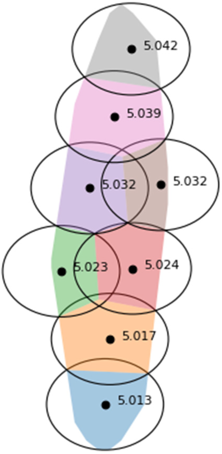
Using the Voronoi diagram and Voronoi iteration process, the optimal spray points were calculated for each stressed region.
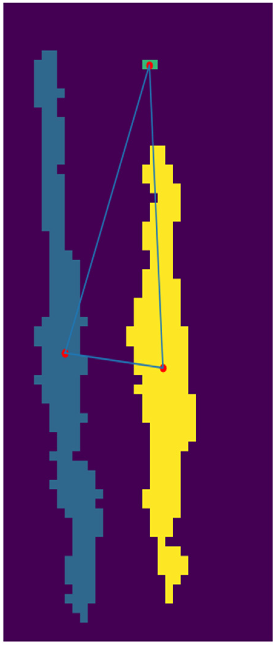
Thereafter, the shortest path from the starting point traversing through each stressed region and its spray points was found using a TSP-based route planning solution.
The next step of the process involved the identification of stressed and unhealthy regions from the spectral images. As discussed in the previous sections, we used the VegNet software to identify the stressed regions [33]. These stressed regions indicated some sort of deficiencies which could be reduced with the help of appropriate fertilizers. The proposed method of spraying with UAVs took into consideration that an equal quantity of spray would be administered irrespective of the degree of deficiency. To decide the equipment to be used for spraying, parameters such as the radius and area to be covered in single spray and the type and quantity of fertilizer to be sprayed were considered.
When the thresholds were identified and applied to the spectral image, the stressed areas were obtained using VegNet software application. These stressed regions were small regions in the farm separated from each other by some distance. These were then extracted to get the individual stressed regions. The flood filling method is one of two popular methods for extraction of individual regions in a binary image. In this method, a region is filled in all directions starting from a single point within the region. This method searches for an unlabeled foreground pixel, labels it and marks it “visited” to all the neighboring pixels in the region [71,72].
In this method, the 8-connected component was used as a metric for the identification of connected image regions. Hence, by employing the flood filling algorithm, each stressed region could be obtained. Therefore, later on, the centroid of each stressed region could be obtained from these stressed regions.
The next procedure involved finding the shortest path from the starting point and traversing through each stressed region’s centroid. Therefore, this method found the shortest path through each stressed region and then, for each stressed region, the shortest path for traversing each spray region was determined. The problem of finding the shortest path through each of these points is called the TSP. The travelling salesman is a classical problem in computer science and operations research. It can be described as a graph with N nodes. All the nodes are connected to each other with an edge that has a corresponding weight and cost attached to it. The cost describes how “difficult” it is to traverse this edge on the graph. The objective of the salesman is to visit all the N cities (nodes) by visiting each node only once, finishing where he started and keeping the traversal costs as low as possible. Since there are N factorial combinations for N nodes, it is impossible to go through all the possible combinations if N is large; therefore, some scientific methods have been formed for solving the problem. Some of the popular ones are the Branch and Bound algorithm [73] and local search algorithms, such as the 2-opt algorithm [74]. In 1975, Chisman used a variation of the travelling salesman problem called the clustered travelling salesman problem [75]. Here, a group of nodes (clusters) must be visited contiguously in an optimal order. There exist several sets of clusters within the problem. This method was developed for optimizing, simultaneously, the ordering of nodes within each cluster and the ordering of clusters. Therefore, in our problem, the stressed regions act as clusters while the spray points inside them are the nodes of each cluster.
In order to find the spray points for each stressed region, their boundary was calculated. This was performed with the help of mathematical morphological operations. The boundaries of the stressed regions inside spectral image A can be calculated as A—(A Θ B) where B is a 3 × 3 square structuring element. Here (A Θ B) denotes erosion of A by B where erosion is another mathematical morphological operation [76,77]. Figure 4 shows the boundary of the stressed region identified in the study site.
The boundary points obtained from each stressed region were used to find a convex hull for the points. A convex hull is the smallest convex set that contains a set of points enclosed within it. Figure 7 shows the boundary as well as the corresponding convex hull of the stressed region. A convex hull is a primary requirement for implementing the algorithm proposed in this paper. The aim of the convex hull is to make the structure of the stressed region into the shape of a polygon that resembles the original shape while containing all the stressed regions inside of it. The convex polygon shape would help in the storage, manipulation and analysis of these stressed regions as opposed to earlier work with images. There are many algorithms called convex hull algorithms that are used to achieve the convex hull. Some of the popular ones are the Graham scan algorithm proposed by [78] and the gift-wrapping algorithm developed by Jarvis [79]. The algorithm given below is the Graham scan algorithm.

3.3. Graham Scan Algorithm

In Algorithm 1, ccw (counterclockwise) is a function which denotes the counterclockwise rotation. ccw > 0 if three points make a counterclockwise turn clockwise if ccw < 0, and collinear if ccw = 0.
The method utilizes the unique approach of covering each region with circles, with the idea borrowed from the covering of convex regions by base stations towers used in telecommunications [80]. This idea was introduced in the context of mobile communication for efficient base station placement problems in a convex region such that each point in the convex region is covered by at least one base station of equal radius. The present research is based on the above idea, with the convex region being the stressed region and the base station being the location where the fertilizer has to be applied, optimizing the base station location for the k points [80].
Algorithm 1. Function GrahamScanAlgorithm(points)
points = list of points
stack = EmptyStack()

P0 = lowest y-coordinate and leftmost point
sort points by polar angle with P0, if several points have the same polar angle then only keep the farthest
for point in points:
  while count stack > 1 and ccw(next_to_top(stack), top(stack), point) < 0:
    stack.pop()
  stack.push(point)
return stack
End
Since finding the number of points for spreading is also a task, this method was applied iteratively and the points were increased one by one till almost all of the convex region was covered and the maximum circumscribing radius was obtained, approximately equal to the radius chosen for the spray. The algorithm initially started with a rough estimate of the number of points needed to cover the convex region, i.e., equal to the total area of the convex region divided by the area of the spray. Then, the number of points was increased iteratively and optimized until most of the stressed area was covered by spray, i.e., 97% of stressed region in our case, and the maximum radius of the enclosed circle was less than or equal to the radius of the spray. We chose 97% in our case because we wanted to find a balance between the minimum number of circles required to cover a region and to cover the maximum amount of area. The number of points, as well as their location, was the answer which was finally obtained. Table 2 shows the number of spray points and area of the stressed region not covered by spray in the selected region after completion of optimization processes. This table shows that eight points were selected, covering more than 97% of the stressed region and had a maximum circumscribing radius equal to the spray radius. Thus, eight points and their optimized locations became the answer for that particular stressed region. These points were further used for route planning, See Algorithm 2.
Algorithm 2. Function find_optimum_points(convex_region, spray_radius)
Number of points (N) = floor(area of convex region/pi* spray_radius * spray_radius)
while True:
Points (P) = Find N random points inside the convex region
Points (P), max_radius = optimum_location_algorithm(convex_region, points, spray_radius)
If ((area_covered_by_points(convex_region, spray_radius) > 97%) and (max_radius =< spray_radius))
return Points (P)
Else:
Number of points (N) = (N) + 1
End

3.4. Voronoi Diagram

The fundamental data structure used in this method is the Voronoi diagram [81] of the point set P, (P is the list of points in the convex region), denoted by VOR(p) for formulating the update mechanism of the members in P to achieve optimum placement. VOR(p) divides the convex region Π into n disjoint convex polygon region such that:
(i)
each region contains a member of P;
(ii)
the region containing point Pi P is denoted by vor(pi);
(iii)
for any arbitrary point q inside a Voronoi region, i.e., q vor(qi), (pi, q) δ(pj, q) <= for all pj ϵ P. Here, δ(p,q) denotes the Euclidean distance of the pair of points.
In this paper, we consider vor(qi) as a closed convex region for each point. So, if a part of the region is outside the convex region then vor(qi)∩Π is used as vor(qi).
The way to optimize the points in the region is to find the positions of all the points P inside the region such that the maximum range required is as quickly as possible. The algorithm is iterative, so it perturbed the points P until it finally attained a local minimum. This algorithm is also called the Voronoi iteration algorithm or Lloyd’s algorithm [82]. At each iteration, a circumscribing circle (Ci) for each vor(pi) was calculated using the algorithm [83]. Ri became the radius of the circumscribing circle (Ci). In order to cover a convex polygon by a spray with a minimal range, the spray should be placed at the center of the circumscribed polygon of the convex region and assigned a range of spray equal to the radius of the circle. As such, the maximum radius was calculated for all the circumscribing circles, which was equal to ρ . This maximum radius was minimized until the circle radius matched the spray radius and the number of iterations did not exceed the limit, i.e., cross the particular value of 40 in our case. We choose 40 in this case because most of the optimizations take place in the first few iterations; after that it converges to another value. The last iterations would lead to a very small decrease in the maximum radius, which is the value that we were optimizing (see Table 3). Therefore, 40 iterations ensured that only major iterations took place in the algorithm and reduced the time for running further optimization processes.
The number of points was increased iteratively until most of the stressed area was covered with a spray, i.e., 97% of stressed region in our case, and the maximum radius of the enclosed circle was less than or approximately equal to the radius of the spray. If these spray point positions covered more than 97% of the area and had a maximum radius which was less than or equal to the spray radius, then these points became the spray points of the stressed region.

3.5. Voronoi Iteration Algorithm or Lloyd’s Algorithm

Lloyd’s algorithm starts with an initial placement of some number k of points. It then repeatedly executes the following relaxation steps:
  • The Voronoi diagram of the k sites is computed.
  • Each cell of the Voronoi diagram is integrated and the centroid is computed.
  • Each site is then moved to the centroid of its Voronoi cell.
This relaxation step terminated when the new set of points met some convergence criteria. Algorithm 3 was very crucial in obtaining the optimum location of these points so that the spray radius would become equal to the maximum circumscribing radius of the region.
Algorithm 3. Function optimum_location_algorithm(convex_region, points, spray_radius)
set of points P   =   { p 1 ,   p 2 ,   ....   p k   }   inside the convex polygon.
iter_count = 0
ρ (maximum radius) = 0
while iter_count < 40 and ρ > spray_radius
  Find the voronoi diagram for the points P
  Compute the circumscribing circle C i   f or each v o r ( p i )
   r i be the radius of C i
  Move p   i to the center of C i and assign range r i   o to it
             ρ   =   =   m a x { r i   ,   i   =   1 ,   2   }
  iter_count += 1
return Points (P), (maximum radius) ρ
End
After finding the locations for the application of fertilizer for a particular stressed region, the TSP-based algorithm was, again, applied to obtain the shortest path traversing all the points. When the drone had traversed all the points in the stressed region, it then moved on to the next stressed region. Figure 9 shows the stressed region along with spray points and spray regions in the stressed region. Figure 11 shows the optimized path through all the stress points in the region.
Most drones today are configured with mission planner software which can be used to create automated missions. This is done by programming the micro-controller manually or programmatically to automated paths using the input of latitude, longitude, altitude and time delays. This automated mission ensures that these drones would not have to be controlled manually thus removing any risk of a crash or manual error. Ardu Pilot’s Mission Planner software has the ability to create automated paths using Python scripts [84].

4. Results and Discussion

This section discusses the outcomes derived from the paper, i.e., finding the optimal points for spraying stressed regions and the optimal path to follow while covering all possible points in the field without re-visiting single points. For assessing the stress regions, a combination of spectral indices or thermal indices were obtained as per user needs and requirements, or the user could employ any techniques or methods to assess the stressed regions. Results will demonstrate the advantages of using TSP-based algorithms using UAVs within agricultural plots to reduce associated costs with labor and fertilizer spraying, thereby realizing the goal of this study for optimal route to visit each stressed point only once, and cover the entire agricultural area in a minimum time interval.
As discussed in previous sections, VegNet software helped in providing the stressed location and regions of stress in the farm holdings (please refer to [33]). Figure 3 illustrates the stressed regions identified in the agricultural regions, highlighted with yellow color, and the blue color represents the non-stressed regions. Figure 3a represents whole agricultural fields while Figure 3b illustrates a very small part of the agricultural holdings. We thus had this small piece of agriculture field to which we applied the algorithm present in this paper. Figure 4 shows the optimum route to be taken to reach each stressed region, which was obtained after applying an algorithm for solving this problem of clustered TSP. Figure 4 demonstrates the application of the (Travelling salesman) TS algorithm on the stressed regions in the agricultural field in order to find the optimum path to each stressed region. Each stressed region is illustrated with a different color and the blue line shows the optimal path to the centroid of each stressed region.
Using flood filling algorithms, we selected stressed regions from the cluster of stressed regions, as shown in Figure 5. Thereafter, the boundary of each stressed region was delineated from the selected region. The delineated boundaries of the stressed regions can be seen in Figure 6. Thereafter comes the role and importance of the convex hull, which uses the delineated boundaries of the stressed regions in order to get a polygon that resembles their original shapes. The convex shape helps in the storage, manipulation and analysis of stressed regions which is a primary requirement for implementing the proposed algorithm. A typical convex hull applied on the delineated boundary of the stressed region can be seen in Figure 7.
The algorithm then estimated the minimum number of circles required for covering the stressed region using the stressed region’s area and the area of spray region. Let this number be N. Then, N random points were found in the stressed region. For these random points, a Voronoi diagram was made and the corresponding circumscribing circles (for each region of the Voronoi diagram) were obtained. Then began the iterative optimization process where the locations of the points kept on updating so that a minimum number of sprays was required to cover a stressed region. The number of points was increased iteratively until most of the stressed area was covered with spray, i.e., 97% of the stressed region, and the maximum radius of the enclosed circle was less than or approximately equal to the radius of the spray. If these spray points positions covered more than 97% of the area and had a maximum radius which was less than or equal to the spray radius, then these points became the spray points of the stressed region.
Table 2 shows the number of spray points and area of the stressed region not covered by spray in the selected region after the optimization process. This table shows that as the number of points was increased, the percentage of stressed region area not covered by the spray region decreased. When eight points were selected, more than 97% of the stressed area was covered and had a maximum radius less than or equal to the spray radius. If the number of points was increased after this, then there was a very marginal decrease in the percentage of stressed region area not covered by the spray region. On the other hand, there would be a large requirement of spray liquid which would lead to overuse of fertilizer and pesticides. Table 3 shows the optimization steps when eight spray points were selected. The maximum circumcircle radius kept on decreasing in each step until there was very little change in the last few steps where the algorithm ended. Figure 8 shows the Voronoi diagram and the corresponding circumscribing circles after optimization, where different regions of Voronoi are shown with different colors. Here, the maximum radius of the circumscribing circle was 5.046 units, i.e., 40.4 cm, which is shown in the last step of optimization in Table 3. The maximum radius of the circumscribing circle, i.e., 40.4 cm, was almost equal to the spray radius from the UAVs, i.e., 40 cm (1 unit = 1 pixel = 8 cm).
This optimization provides optimal points in the stressed regions which uses these points to provide the optimal path and route to deliver services in the fields at appropriate points with accuracy. Thus, optimal points are required to ensure the route of the UAVs to reach at each point without re-visiting the same place in its complete trip. In our study, optimum route was identified using TSP based algorithm and Voronoi Diagram which has been illustrated in Figure 9. Thus, Figure 9 shows the coverage of the stressed crops with a fixed amount of radius i.e., radius of the spray from UAVs. In our case study, the optimal route has been shown in the application of UAVs for spraying the fertilizer at each point and spray radius of fertilizer by UAVs equal to 0.4 m (as shown in Figure 9). Here, all the circles will be of the same radius. We have also provided the different stressed regions in Figure 10a and illustrated how Drone is covering all the three types of stressed regions along with overlap areas. Table 4 provides the information about the overlap regions for these three stressed regions (based on the area covered by stressed regions). Therefore, this optimal points and optimal path route will use the shortest possible route to cover the agricultural fields completely in possibly less time frame. The advantages of this study is that it will provide the coverage of entire field in a minimum period with full coverage without re-visiting. Figure 11 indicates the optimal route through all spray points in the stressed region with a fixed spray radius of 40 cm. Hence, the optimised path is derived through all the spray points generated using TSP based algorithms.
A few important studies can be highlighted here that briefly demonstrated the spraying of fertilizers and pesticides on farms of a particular shape and size, which were easy to maneuver, and design algorithms. In 2013, one article demonstrated the optimization of maneuvering near boundaries and the loading and unloading of inputs of an agricultural machine [85]. The method suggested works only for specific field geometries with all parts of the field being sprayed irrespective of whether an area is stressed or not. Furthermore, previous papers divided the stressed regions into various small rectangles for spraying, but this shape is not the most appropriate one for spraying since the spraying happens over a circular area. Therefore, a circular shape was chosen for dividing the stressed region in this study. In comparison, some authors demonstrated easier methods of maneuvering with the help of UAVs. Similarly, Cabreira et al. [58] discussed coverage path planning to cover every region of interest considering the different area shapes [58]. Some others discussed algorithms, such as back-and-forth coverage path planning algorithms, which are suitable for continuous spraying in a region. These algorithms used turning maneuvers which increased the time and energy spent at corners, thus giving irregular spraying at the corners of the regions. One article discussed the development of a coverage trajectory with a minimal required time for UAVs for better navigation for any specific task [60]. Here, the authors used rectangular grids to divide a stressed region and then used path planning algorithms to find an optimized path. However, it is not the best idea to divide a stressed region which has a very irregular shape into rectangular grids. This is because the grids might contain areas which do not require these inputs which leads to unnecessary spraying. These grid-based spray systems would not be optimal as applying a circular spray motion on a rectangular cell is not preferred. This may lead to missed spraying or over-spraying in some areas.
This paper will help to spray inputs only on the stressed area where it is required and where there is nutrient deficiency. We also suggest spraying inputs while the UAV is flying still over the spray position. This method of spraying would reduce some of the spraying factors associated with UAVs. We have tried to combine all the shortcomings from earlier research to come out with an algorithm for proper spraying of pesticides by drones which provides continuous feedback to the system for allowing spraying of fertilizers on all shapes of stressed regions. Finally, the algorithm outputs an optimized route covering all the stressed regions and spray points. The tasks of administering pesticides and fertilizer, when done by traditional means, take a lot of time and are not efficient processes. However, by using the proposed method, the task of administering fertilizer and pesticide can be completed in a shorter time frame, with optimum resources and with a high level of accuracy.

5. Challenges

This section deals with the challenges and hurdles associated with the UAVs and discusses the future work scope, conclusion and recommendations. There are numerous challenges associated with UAVs which will be the main focus before delivering the application part for the optimal path and route. The first challenge is the usage of drones as they are more difficult to control as they move rapidly in all possible directions, and they can be difficult to control in adverse weather conditions, such as rain or high wind turbulence. However, most drones now come with automated navigation software that enables autonomous flight, requiring no input from the user apart from route instructions. The UAV’s size and weight are also challenges to the user, along with their operational flight time, which depend upon the battery being used. Drones have a limited battery capacity; therefore, they have a short time flight. To compensate for this, larger batteries can be used which makes them more expensive. UAVs also cannot carry a heavy load; therefore, they would need to be refilled with inputs and their batteries recharged before flying again. Therefore, the resupply trips should be incorporated into the route planning, depending on the type of input being administered and size of the field. Drones also require a large memory for storing and processing high resolution spectral images. Drone operations are heavily regulated by most governments and require a license to be operated in certain regions and places due to security and safety issues. Along with challenges in the hardware, there exist some challenges with the software too, despite the presence of a large number of open-source libraries for the implementation of software and availability of affordable graphical processing units (GPUs). Irrespective of the above-mentioned challenges, UAVs are widely used by overcoming these challenges, somehow, either by using a short flight duration, low spectral resolution data (not acquiring hyperspectral data) or by spending money on expensive batteries to operate over large land holdings.

6. Future Work

This section deals with future research directions. In this paper, a simple method of fertilizer and pesticide application by drone has been discussed which automates the process of identification and application of fertilizer automatically, without any need for human decision-making and manual labor. This paper used only one of the many vegetative indexes available in the research literature for finding stressed regions with a deficiency of a particular nutrient. The future work of this paper could be the integration of various kinds of vegetative indices which indicate various kinds of nutrient deficiencies. These deficiencies could be used to predict the overall health of the crop. This paper proposes a method for spraying only one fertilizer at a time, but the method could be developed so that multiple fertilizers and pesticides could be sprayed onto the stressed region, thus improving the process efficiency and reducing the cost. This would result in a reduction in the number of steps which need to be taken to find and rectify each deficient nutrient, while a centralized system could be developed to address all the deficiencies with a single spray of fertilizers/pesticides. As agricultural machines spend a significant part of their time on non-productive operations, with more time spent on turns and repetitions, the technique described will help to reduce these non-productive operations.
This paper focused on administering an equal amount of fertilizer to the stressed region irrespective of the degree of nutrient deficiency. However, ideally, there should be a focus on applying the fertilizer based on the degree of fertilizer and nutrient deficiency. Therefore, a novel method will be much needed in the future which can administer fertilizer based on the degree of deficiency of fertilizers in respect to volume requirement. This method could lead to the development of more sophisticated software, with which farmers can estimate their total revenue and losses due to the stressed regions. This could be done by integrating various kinds of real-time global prices and real-time sensor data with the yield prediction data obtained through the drone. Another future scope is the usage of artificial intelligence which is being used in a wide range of complex tasks, ranging from speech processing to self-driving cars and, more recently, in geospatial applications (remote sensing and geographical information systems). Many artificial intelligence applications are currently being researched and developed to use hyperspectral data for prediction of the yield and health of crops. These data could be used for PA activities and would help in increasing the agricultural crop yields and income. Autonomous UAVs have great potential to exploit agricultural applications to improve and enhance crop yields and productivity, with improved accuracy in spraying route and higher time efficiency, as well proper coverage. This applicability can be applied to other research domains as well, such as forestry, ocean and defense. Another suitable application could be the use of this method for extinguishing forest fires that could be detected by UAVs. This method can help to timely extinguish fires and prevent them from spreading using optimal route calculation and maintaining the route of interest by not deviating from optimum path. With the more advanced development of UAVs which are capable of lifting higher loads, this method can be used for precision irrigation so that the optimum amount of water can be used.

7. Conclusions and Recommendations

The paper discussed the results, challenges and future scopes of the methodology for using UAVs in precision agriculture. The results demonstrated the advantages of using TSP algorithms for UAVs within agricultural plots to reduce associated costs with labor and fertilizer spraying. This paper described a method by which automated UAVs can be used efficiently in providing inputs, such as pesticides and fertilizers, for precision agriculture. The method uses optimal points and route to provide these inputs to the stressed regions of the farm, thus covering the entire agricultural area using optimal amounts of inputs over a minimal distance and in minimum time. These optimal outcomes are generated from TSP-based algorithms and Voronoi diagrams implemented on spectral images acquired through UAVs. The spectral images are employed to locate and assess the stressed regions in large landholdings, using a spectral indices-based application (for details, refer to [33]). A few recommendations for future work using UAVs for PA applications that can be used by farmers to enhance crop yields (prevent crop damage) have also been given. Some of the recommendation points are listed below:
-
Employ a combination of spectral indices or thermal indices to assess the stress regions in terms of soil moisture, nutrient deficiency and disease condition.
-
Employ any techniques or methods to assess the stressed regions which employ accurate methods and applications for the above.
-
Utilize route planning and an optimal path that can be used in any field shape and size.
-
Implement an optimal path and route for other agricultural applications, such as pesticides and insecticides.
-
Implement these techniques while sowing the seeds, effectively and in proper rows.
-
Use advanced techniques of calculating an optimal path and route during harvesting to manage large landholdings to make it cost effective and time-saving.
Implementation of the points outlined above would greatly improve the productivity of large landholdings and farms while decreasing the need for manual labor and repetitive concerns for stressed point location through remote sensing application instead of knowledge-based field visiting information. In this paper, we concluded with a key recommendation to employ UAVs to find an optimized route to completely cover stressed areas efficiently and without wastage of input resources during the spraying process which is tackled with the TSP solving technique. However, there is a need for evolving much more efficient algorithms for a true sense of PA in a sustainable way to meet the future requirements of PA.

Author Contributions

Conceptualization, P.C.P.; Data curation, K.S.; Methodology, K.S.; Project administration, P.C.P.; Resources, K.S. and P.C.P.; Software, K.S.; Supervision, P.C.P. and J.K.S.; Validation, K.S.; Visualization, K.S. and P.C.P.; Writing—original draft, K.S. and P.C.P.; Writing—review and editing, P.C.P. and J.K.S. All authors have read and agreed to the published version of the manuscript.

Funding

This research received OUR Shiv Nadar University funding.

Acknowledgments

The authors are thankful to Shiv Nadar University for providing the research facilities.

Conflicts of Interest

The authors declare no conflict of interest.

References

  1. United Nations. Sustainable Development Website—United Nations. Food Security and Nutrition and Sustainable Agriculture. 2019. Available online: https://sustainabledevelopment.un.org/topics/foodagriculture (accessed on 13 March 2019).
  2. United Nations Population. Global Issues—Population Website—United Nations. 2019. Available online: https://www.un.org/en/sections/issues-depth/population/ (accessed on 13 March 2019).
  3. Bruinsma, J. The resource outlook to 2050: By how much do land, water and crop yields need to increase by 2050. Expert Meet. How Feed World 2009, 2050, 24–26. Available online: http://www.fao.org/3/a-ak971e.pdf (accessed on 20 February 2020).
  4. Millennium Ecosystem Assessment. Ecosystems and Human Well-Being; Island Press: Washington, DC, USA, 2005; Volume 5. [Google Scholar]
  5. Goodland, R. The concept of environmental sustainability. Ann. Rev. Ecol. Syst. 1995, 26, 1–24. [Google Scholar] [CrossRef]
  6. WHO. Ecosystems and Human Well-Being, Health Synthesis. 2005. Available online: http://www.bioquest.org/wp-content/blogs.dir/files/2009/06/ecosystems-and-health.pdf (accessed on 20 August 2019).
  7. Lamine, S.; Petropoulos, G.P.; Brewer, P.A.; Srivastava, P.K.; Bachari, N.E.; Manevski, K.; Kalaitzidis, C.; Macklin, M.G. Heavy Metal Soil Contamination Detection Using Combined Geochemistry and Field Spectroradiometry in the United Kingdom. Sensors 2019, 19, 762. [Google Scholar] [CrossRef] [PubMed] [Green Version]
  8. Sharma, L.; Pandey, P.C.; Nathawat, M. Assessment of land consumption rate with urban dynamics change using geospatial techniques. J. Land Use Sci. 2012, 7, 135–148. [Google Scholar] [CrossRef]
  9. Pandey, P.C.; Mandal, V.; Katiyar, S.; Kumar, P.; Tomar, V.; Patairiya, S.; Ravisankar, N.; Gangwar, B. Geospatial Approach to Assess the Impact of Nutrients on Rice Equivalent Yield Using MODIS Sensors’-Based MOD13Q1-NDVI Data. IEEE Sens. J. 2015, 15, 6108–6115. [Google Scholar] [CrossRef]
  10. Mondal, P.; Basu, M. Adoption of precision agriculture technologies in India and in some developing countries: Scope, present status and strategies. Prog. Nat. Sci. 2009, 19, 659–666. [Google Scholar] [CrossRef]
  11. Tey, Y.S.; Brindal, M. Factors influencing the adoption of precision agricultural technologies: A review for policy implications. Precis. Agric. 2012, 13, 713–730. [Google Scholar] [CrossRef]
  12. Thomas, D.E.; Weyerhaeuser, H.; Saipathong, P.; Onpraphai, T. Negotiated land use patterns to meet local and societal needs. In Proceedings of the Cultures and Biodiversity Congress 2000, Yunnan, China, 20–30 July 2000; Yunnan Science and Technology Press: Yunnan, China, 2000; pp. 414–433. Available online: http://old.worldagroforestry.org/downloads/Publications/PDFS/PP00160.pdf (accessed on 15 March 2020).
  13. Mogili, U.R.; Deepak, B.B.V.L. Review on Application of Drone Systems in Precision Agriculture. Procedia Comput. Sci. 2018, 133, 502–509. [Google Scholar] [CrossRef]
  14. Somayeh Tohidyan, F.; Rezaei-Moghaddam, K. Impacts of the precision agricultural technologies in Iran: An analysis experts’ perception & their determinants. Inf. Process. Agric. 2018, 5, 173–184. [Google Scholar] [CrossRef]
  15. Whelan, B.M.; McBratney, A.B.; Boydell, B.C. The Impact of Precision Agriculture. In Proceedings of the ABARE Outlook Conference, the Future of Cropping in NW NSW, Moree, UK, 15 July 1997; p. 5. [Google Scholar]
  16. Mulla, D.J. Twenty five years of remote sensing in precision agriculture: Key advances and remaining knowledge gaps. Biosyst. Eng. 2013, 114, 358–371. [Google Scholar] [CrossRef]
  17. Schnug, E.; Panten, K.; Haneklaus, S. Sampling and nutrient recommendations—The future. Commun. Soil Sci. Plant Anal. 1998, 29, 1455–1462. [Google Scholar] [CrossRef]
  18. Singh, P.; Pandey, P.C.; Petropoulos, G.P.; Pavlides, A.; Srivastava, P.K.; Koutsias, N.; Kwal Deng, K.A.; Yangson, B. Hyperspectral remote sensing in precision agriculture: Present status, challenges, and future trends. In Hyperspectral Remote Sensing: Theory and Applications; Pandey, P.C., Srivastava, P.K., Baltzer, H., Eds.; Elsevier: Amsterdam, The Netherlands, 2020; Chapter 8; pp. 121–146. [Google Scholar] [CrossRef]
  19. Bagheri, N.; Ahmadi, H.; Alavipanah, S.K.; Omid, M. Multispectral remote sensing for site-specific nitrogen fertilizer management. Pesqui. Agropecu. Bras. 2013, 48, 1394–1401. [Google Scholar] [CrossRef] [Green Version]
  20. Wójtowicz, M.; Wójtowicz, A.; Piekarczyk, J. Application of remote sensing methods in agriculture. Commun. Biometry Crop Sci. 2016, 11, 31–50. [Google Scholar]
  21. Hruska, R.C.; Mitchell, J.J.; Anderson, M.; Glenn, N.F. Radiometric and Geometric Analysis of Hyperspectral Imagery Acquired from an Unmanned Aerial Vehicle. Remote Sens. 2012, 4, 2736–2752. [Google Scholar] [CrossRef] [Green Version]
  22. Uto, K.; Seki, H.; Saito, G.; Kosugi, Y. Characterization of Rice Paddies by a UAV-Mounted Miniature Hyperspectral Sensor System. IEEE J. Sel. Top. Appl. Earth Obs. Remote Sens. 2013, 6, 851–860. [Google Scholar] [CrossRef]
  23. Zarco-Tejada, P.J.; Gonzalez-Dugo, V.; Berni, J.; Jimenez-Berni, J.A. Fluorescence, temperature and narrow-band indices acquired from a UAV platform for water stress detection using a micro-hyperspectral imager and a thermal camera. Remote Sens. Environ. 2012, 117, 322–337. [Google Scholar] [CrossRef]
  24. Stehr, N.J. Drones: The Newest Technology for Precision Agriculture. Nat. Sci. Educ. 2015, 44, 89–91. [Google Scholar] [CrossRef]
  25. Von Bueren, S.K.; Burkart, A.; Hueni, A.; Rascher, U.; Tuohy, M.P.; Yule, I.J. Deploying four optical UAV-based sensors over grassland: Challenges and limitations. Biogeosciences 2015, 12, 163–175. [Google Scholar] [CrossRef] [Green Version]
  26. Gago, J.; Douthe, C.; Coopman, R.; Gallego, P.P.; Ribas-Carbo, M.; Flexas, J.; Escalona, J.; Medrano, H. UAVs challenge to assess water stress for sustainable agriculture. Agric. Water Manag. 2015, 153, 9–19. [Google Scholar] [CrossRef]
  27. Honkavaara, E.; Saari, H.; Kaivosoja, J.; Pölönen, I.; Hakala, T.; Litkey, P.; Mäkynen, J.; Pesonen, L. Processing and Assessment of Spectrometric, Stereoscopic Imagery Collected Using a Lightweight UAV Spectral Camera for Precision Agriculture. Remote Sens. 2013, 5, 5006–5039. [Google Scholar] [CrossRef] [Green Version]
  28. Schmale David, G., III; Dingus, B.R.; Reinholtz, C.; Schmale, D.G. Development and application of an autonomous unmanned aerial vehicle for precise aerobiological sampling above agricultural fields. J. Field Robot. 2008, 25, 133–147. [Google Scholar] [CrossRef]
  29. Cheein, F.A.A.; Carelli, R. Agricultural Robotics: Unmanned Robotic Service Units in Agricultural Tasks. IEEE Ind. Electron. Mag. 2013, 7, 48–58. [Google Scholar] [CrossRef]
  30. Freeman, P.K.; Freeland, R.S. Agricultural UAVs in the U.S.: Potential, policy, and hype. Remote Sens. Appl. Soc. Environ. 2015, 2, 35–43. [Google Scholar] [CrossRef]
  31. Nebiker, S.; Annen, A.; Scherrer, M.; Oesch, D. A light-weight multispectral sensor for micro UAV—Opportunities for very high resolution airborne remote sensing. Int. Arch. Photogramm. Remote Sens. Spat. Inf. Sci. 2008, 37, 1193–1199. [Google Scholar]
  32. Fischer, A. A model for the seasonal variations of vegetation indices in coarse resolution data and its inversion to extract crop parameters. Remote Sens. Environ. 1994, 48, 220–230. [Google Scholar] [CrossRef]
  33. Srivastava, K.; Bhutoria, A.J.; Sharma, J.K.; Sinha, A.; Pandey, P.C. UAVs technology for the development of GUI based application for precision agriculture and environmental research. Remote Sens. Appl. Soc. Environ. 2019, 16, 100258. [Google Scholar] [CrossRef]
  34. Huete, A. A soil-adjusted vegetation index (SAVI). Remote Sens. Environ. 1988, 25, 295–309. [Google Scholar] [CrossRef]
  35. Horler, D.N.H.; Dockray, M.; Barber, J. The red edge of plant leaf reflectance. Int. J. Remote Sens. 1983, 4, 273–288. [Google Scholar] [CrossRef]
  36. Huete, A.R.; Liu, H.Q.; Batchily, K.V.; Van Leeuwen, W. A comparison of vegetation indices over a global set of TM images for EOS-MODIS. Remote Sens. Environ. 1997, 59, 440–451. [Google Scholar] [CrossRef]
  37. Haboudane, D.; Miller, J.R.; Tremblay, N.; Zarco-Tejada, P.J.; Dextraze, L. Integrated narrow-band vegetation indices for prediction of crop chlorophyll content for application to precision agriculture. Remote Sens. Environ. 2002, 81, 416–426. [Google Scholar] [CrossRef]
  38. Gonçalves, J.A.; Henriques, R. UAV photogrammetry for topographic monitoring of coastal areas. ISPRS J. Photogramm. Remote Sens. 2015, 104, 101–111. [Google Scholar] [CrossRef]
  39. Pinto, E.; Santana, P.; Barata, J. On collaborative aerial and surface robots for environmental monitoring of water bodies. In Doctoral Conference on Computing, Electrical and Industrial Systems; Springer: Berlin/Heidelberg, Germany, 2013; pp. 183–191. [Google Scholar]
  40. Watanabe, Y.; Kawahara, Y. UAV Photogrammetry for Monitoring Changes in River Topography and Vegetation. Procedia Eng. 2016, 154, 317–325. [Google Scholar] [CrossRef] [Green Version]
  41. Li, C.-C.; Zhang, G.-S.; Lei, T.-J.; Gong, A.-D. Quick image-processing method of UAV without control points data in earthquake disaster area. Trans. Nonferrous Met. Soc. China 2011, 21, s523–s528. [Google Scholar] [CrossRef]
  42. Matese, A.; Toscano, P.; Di Gennaro, S.F.; Genesio, L.; Vaccari, F.P.; Primicerio, J.; Belli, C.; Zaldei, A.; Bianconi, R.; Gioli, B.; et al. Intercomparison of UAV, Aircraft and Satellite Remote Sensing Platforms for Precision Viticulture. Remote Sens. 2015, 7, 2971–2990. [Google Scholar] [CrossRef] [Green Version]
  43. Muzari, W.; Gatsi, W.; Muvhunzi, S. The Impacts of Technology Adoption on Smallholder Agricultural Productivity in Sub-Saharan Africa: A Review. J. Sustain. Dev. 2012, 5, 69. [Google Scholar] [CrossRef]
  44. Anderson, K.R. A reevaluation of an efficient algorithm for determining the convex hull of a finite planar set. Inf. Process. Lett. 1978, 7, 53–55. [Google Scholar] [CrossRef]
  45. Xuemei, L.; Yuyan, D.; Lixing, D. Study on precision agriculture monitoring framework based on WSN. In Proceedings of the 2008 2nd International Conference on Anti-Counterfeiting, Security and Identification, Guiyang, China, 20–23 August 2008. [Google Scholar]
  46. López-Riquelme, J.; Pavón-Pulido, N.; Navarro-Hellín, H.; Soto-Valles, F.; Torres-Sánchez, R. A software architecture based on FIWARE cloud for Precision Agriculture. Agric. Water Manag. 2017, 183, 123–135. [Google Scholar] [CrossRef]
  47. Nash, E.; Korduan, P.; Bill, R. Applications of open geospatial web services in precision agriculture: A review. Precis. Agric. 2009, 10, 546–560. [Google Scholar] [CrossRef]
  48. Hunt, E.R.; Hively, W.D.; Daughtry, C.S.; McCarty, G.W.; Fujikawa, S.J.; Ng, T.L.; Tranchitella, M.; Linden, D.S.; Yoel, D.W. Remote sensing of crop leaf area index using unmanned airborne vehicles. In Proceedings of the Pecora 17—The Future of Land Imaging, Going Operational, Denver, CO, USA, 18–20 November 2008. [Google Scholar]
  49. Burema, H.; Filin, A. Aerial Farm Robot System for Crop Dusting, Planting, Fertilizing and Other Field Jobs. U.S. Patent No. 9,382,003, 5 July 2016. [Google Scholar]
  50. Qin, W.-C.; Qiu, B.-J.; Xue, X.; Chen, C.; Xu, Z.-F.; Zhou, Q. Droplet deposition and control effect of insecticides sprayed with an unmanned aerial vehicle against plant hoppers. Crop. Prot. 2016, 85, 79–88. [Google Scholar] [CrossRef]
  51. Zhou, L.P.; He, Y. Simulation and optimization of multi spray factors in UAV. In Proceedings of the 2016 ASABE Annual International Meeting, Lake Buena Vista, FL, USA, 17–20 July 2016; American Society of Agricultural and Biological Engineers: Saint Joseph, MI, USA, 2016. [Google Scholar] [CrossRef]
  52. Yao, L.; Jiang, Y.; Zhiyao, Z.; Shuaishuai, Y.; Quan, Q. A pesticide spraying mission assignment performed by multi-quadcopters and its simulation platform establishment. In Proceedings of the 2016 IEEE Chinese Guidance, Navigation and Control Conference (CGNCC), Nanjing, China, 12–14 August 2016. [Google Scholar]
  53. Stark, B.; Rider, S.; Chen, Y. Optimal pest management by networked unmanned cropdusters in precision agriculture: A cyber-physical system approach. IFAC Proc. Vol. 2013, 46, 296–302. [Google Scholar] [CrossRef]
  54. Castaldi, F.; Pelosi, F.; Pascucci, S.; Casa, R. Assessing the potential of images from unmanned aerial vehicles (UAV) to support herbicide patch spraying in maize. Precis. Agric. 2016, 18, 76–94. [Google Scholar] [CrossRef]
  55. Campos, J.; Llop, J.; Gallart, M.; García-Ruiz, F.; Gras, A.; Salcedo, R.; Gil, E. Development of canopy vigour maps using UAV for site-specific management during vineyard spraying process. Precis. Agric. 2019, 20, 1136–1156. [Google Scholar] [CrossRef] [Green Version]
  56. Norbert, D. Route Planning System for Agricultural Work Vehicles. U.S. Patent 6,128,574, 3 October 2000. Available online: https://patentimages.storage.googleapis.com/86/bd/48/076423c308fe7b/US6128574.pdf (accessed on 25 June 2020).
  57. Rodias, E.; Berruto, R.; Busato, P.; Bochtis, D.; Sørensen, C.G.; Zhou, K. Energy Savings from Optimised In-Field Route Planning for Agricultural Machinery. Sustainability 2017, 9, 1956. [Google Scholar] [CrossRef] [Green Version]
  58. Cabreira, T.M.; Brisolara, L.B.; Ferreira, P.R., Jr. Survey on Coverage Path Planning with Unmanned Aerial Vehicles. Drones 2019, 3, 4. [Google Scholar] [CrossRef] [Green Version]
  59. Galceran, E.; Carreras, M. A survey on coverage path planning for robotics. Robot. Auton. Syst. 2013, 61, 1258–1276. [Google Scholar] [CrossRef] [Green Version]
  60. Nam, L.H.; Huang, L.; Li, X.J.; Xu, J.F. An approach for coverage path planning for UAVs. In Proceedings of the 2016 IEEE 14th International Workshop on Advanced Motion Control (AMC), Auckland, New Zealand, 22–24 April 2016; pp. 411–416. [Google Scholar] [CrossRef] [Green Version]
  61. Tokekar, P.; Hook, J.V.; Mulla, D.; Isler, V. Sensor Planning for a Symbiotic UAV and UGV System for Precision Agriculture. IEEE Trans. Robot. 2016, 32, 1498–1511. [Google Scholar] [CrossRef]
  62. Tarot. Tarot 4008 Martin Long Flight Time BLDC Motor Specifications. 2019. Available online: http://www.tarotrc.com/Product/Detail.aspx?Lang¼en&Id¼9fc38c24-b74d-469d-b568-3d5ea644874a (accessed on 17 December 2019).
  63. Planner, Mission. Ardupilot—Mission Planner Documentation. 2019. Available online: http://ardupilot.org/planner/index.html (accessed on 5 December 2018).
  64. Alsalam, B.H.Y.; Morton, K.; Campbell, D.; Gonzalez, F. Autonomous UAV with vision based on-board decision making for remote sensing and precision agriculture. In Proceedings of the 2017 IEEE Aerospace Conference, Big Sky, MT, USA, 4–11 March 2017; pp. 1–12. [Google Scholar]
  65. Pixhawk. Pixhawk-4 User Guide and Documentation-PixHawk. 2019. Available online: https://docs.px4.io/v1.9.0/en/flight_controller/pixhawk4.html (accessed on 23 March 2019).
  66. FlySky. FlySky FS-i6S RC Transmitter with Receiver. 2019. Available online: https://www.flysky-cn.com/fsi6s (accessed on 10 November 2019).
  67. U-Blox. U-Blox Neo-7M GPS Module Specifications and Documentation. 2019. Available online: https://www.u-blox.com/en/product/neo-7-series (accessed on 27 January 2019).
  68. Benewafke. Benewake TF02 LiDAR (Mid-Range Distance Sensor) User Guide and Documentation—Benewake. 2019. Available online: http://en.benewake.com/product/detail/5c345c9de5b3a844c4723299 (accessed on 15 February 2019).
  69. MicaSense. MicaSense RedEdge—MX Spectral Camera Specifications. 2019. Available online: https://www.micasense.com/rededge-mx (accessed on 15 November 2019).
  70. Walsh, O.S.; Shafian, S.; Marshall, J.M.; Jackson, C.; McClintick-Chess, J.R.; Blanscet, S.M.; Swoboda, K.; Thompson, C.; Belmont, K.M.; Walsh, W.L. Assessment of UAV Based Vegetation Indices for Nitrogen Concentration Estimation in Spring Wheat. Adv. Remote Sens. 2018, 7, 71–90. [Google Scholar] [CrossRef] [Green Version]
  71. Pavlidis, T. Filling algorithms for raster graphics. Comput. Graph. Image Process. 1979, 10, 126–141. [Google Scholar] [CrossRef]
  72. James, D.F.; Van Dam, A. Fundamentals of Interactive Computer Graphics; Addison-Wesley Longman Publishing Co., Inc.: Boston, MA, USA, 1982; Volume 2, ISBN 0-201-14468-9. [Google Scholar]
  73. Little, J.D.C.; Murty, K.G.; Sweeney, D.W.; Karel, C. An Algorithm for the Traveling Salesman Problem. Oper. Res. 1963, 11, 972–989. [Google Scholar] [CrossRef]
  74. Croes, G.A. A Method for Solving Traveling-Salesman Problems. Oper. Res. 1958, 6, 791–812. [Google Scholar] [CrossRef]
  75. Chisman, J.A. The clustered traveling salesman problem. Comput. Oper. Res. 1975, 2, 115–119. [Google Scholar] [CrossRef]
  76. Serra, J. Image Analysis and Mathematical Morphology; Academic Press: New York, NY, USA, 1982. [Google Scholar]
  77. Soille, P. Morphological Image Analysis, Principles and Applications; Academic Press, Inc.: Orlando, FL, USA, 1999; ISBN 0126372403. [Google Scholar]
  78. Graham, R.L. An efficient algorith for determining the convex hull of a finite planar set. Inf. Process. Lett. 1972, 1, 132–133. [Google Scholar] [CrossRef]
  79. Jarvis, R. On the identification of the convex hull of a finite set of points in the plane. Inf. Process. Lett. 1973, 2, 18–21. [Google Scholar] [CrossRef]
  80. Das, G.K.; Das, S.; Nandy, S.C.; Sinha, B.P. Efficient algorithm for placing a given number of base stations to cover a convex region. J. Parallel Distrib. Comput. 2006, 66, 1353–1358. [Google Scholar] [CrossRef]
  81. De Berg, M.; Van Kreveld, M.; Overmars, M.; Cheong, O. Computational Geometry; Springer: Berlin/Heidelberg, Germany, 1997; pp. 1–17. [Google Scholar] [CrossRef]
  82. Lloyd, S. Least squares quantization in PCM. IEEE Trans. Inf. Theory 1982, 28, 129–137. [Google Scholar] [CrossRef]
  83. Megiddo, N. Linear-time algorithms for linear programming in R3 and related problems. SIAM J. Comput. 1983, 12, 759–776. Available online: http://theory.stanford.edu/~megiddo/pdf/lp3.pdf (accessed on 5 August 2020). [CrossRef]
  84. Mission Planning. Mission Planning—Copter Documentation. 2019. Available online: www.ardupilot.org/copter/docs/common-mission-planning.html (accessed on 25 June 2019).
  85. Spekken, M.; De Bruin, S. Optimized routing on agricultural fields by minimizing maneuvering and servicing time. Precis. Agric. 2012, 14, 224–244. [Google Scholar] [CrossRef]
Figure 1. Schematic diagram illustrating the overall methodology adopted in the present study.
Drones 04 00058 g001
Figure 2. Illustration of the UAV employed in the study.
Drones 04 00058 g002
Figure 3. (a) Stressed regions in the whole agricultural field and (b) a selection of stressed regions for a small region highlighted in yellow.
Drones 04 00058 g003
Figure 4. Applying travelling salesman (TS) on the stressed region, with different stressed regions highlighted by different colors.
Drones 04 00058 g004
Figure 5. A stressed region selected from the cluster of stressed regions (as shown in Figure 3a,b).
Drones 04 00058 g005
Figure 6. Boundary of the stressed region.
Drones 04 00058 g006
Figure 7. Convex hull on the boundary of stressed region.
Drones 04 00058 g007
Figure 8. Voronoi diagram and the corresponding circumscribing circles for Voronoi regions at an iterative optimization step.
Drones 04 00058 g008
Figure 9. Fertilizer spray with radius of 0.40 m on the spray points in the stressed region (here, all the circles are of the same radius).
Drones 04 00058 g009
Figure 10. (a) Stressed regions in test site with different area marked as region I, II and III (based on the area covered) and (b) Path covered for all the stressed regions and their respective spray points (Total Distance covered = 227.73 × 0.08 m = 18.2984 m).
Drones 04 00058 g010
Figure 11. Optimized path through all the spray points in the stressed region.
Drones 04 00058 g011
Table 1. Specifications of the UAV employed in the present study.
Details/Parts of DroneItemsSpecifications
Drone frameFrameCarbon fiber
TypeQuadcopter
Drone motorTypeBrushless direct current motor (BLDC)
Typical endurance40 to 60 min
Weight85 g
Speed330 KV
Digital spectral cameraCamera makeMicaSense Red Edge™ 3 Multispectral Camera
Spectral bandsBlue, green, red, red edge, near-IR
Megapixel3.6 MP
Capture rate1 capture per second
StorageSD card
BatteryTechnologyLithium-ion batteries
Max battery capacity 10,000 mAh
RC controllerMakeFS-i6S transmitter
No. of channels10
Frequency range2.4055–2.475 GHz
Modulation systemGFSK
2.4G modeAFHDS 2A
Light detection and ranging (LIDAR)MakeTF02-Pro 40m IP65 LiDAR
Operating range0.1–40 m
Weight50 g
Frequency1–1000 Hz
GPSOscillatorCrystal
TechnologyGPS, GLONASS
MemoryROM
Navigation update rateup to 10 Hz
PX4 controllerMain chipSTM32F427
CPU180 MHz ARM® Cortex® M4
RAM256 KB SRAM
Connectivity1× I2C, 1× CAN, 1× ADC, 4× UART
SensorsGyroscope, accelerometer, 3-axis gyroscope, barometer
Table 2. Number of spray points in the selected region and area of stressed region not covered by spray after completing the optimization process.
Number of Spray PointsPercentage of Area of Stressed Region Not Covered by Spray RegionRadius of Maximum Circumcircle of a Voronoi Region at the Last Iteration
524.24%0.48712 m
69.14%0.51512 m
75.92%0.45808 m
80.28%0.40368 m
Table 3. Radius of the maximum circumscribing circle for all the iterative optimization steps when N = 8 points were selected for covering a stressed region.
Optimization StepsRadius (in Meters)Optimization StepsRadius (in Meters)Optimization StepsRadius (in Meters)Optimization StepsRadius (in Meters)
10.5572 110.4521210.4212310.4080
20.49120.4470220.4191325.092 0.4073
30.4636130.4429230.4172330.4066
40.4607140.4394240.4156340.4060
50.4628150.4364250.4140350.4056
60.4591160.4336260.4128360.4052
70.4584170.4309270.4116370.4048
80.4576180.4286280.4105380.4044
90.4564190.4260290.4096390.4041
100.4547200.4234300.4088400.4036
Table 4. Statistics for the overlap and area covered for the test site during the optimal route and field coverage (area for overlap for stressed wise percentage).
RegionPercentage of Area Not CoveredPercentage of Area with Overlap
Region I0.04%25.69%
Region II2.12%12.96%
Region III0%0%

