Article

Determining the Optimal Number of Ground Control Points for Varying Study Sites through Accuracy Evaluation of Unmanned Aerial System-Based 3D Point Clouds and Digital Surface Models

Korea Environment Institute, Bldg. B, 370 Sicheong-daero, Sejong 30147, Korea
*
Author to whom correspondence should be addressed.
Drones 2020, 4(3), 49; https://doi.org/10.3390/drones4030049
Submission received: 21 July 2020 / Revised: 15 August 2020 / Accepted: 20 August 2020 / Published: 27 August 2020
(This article belongs to the Special Issue Feature Papers of Drones)

Abstract

:
The rapid development of drone technologies, such as unmanned aerial systems (UASs) and unmanned aerial vehicles (UAVs), has led to the widespread application of three-dimensional (3D) point clouds and digital surface models (DSMs). Due to the number of UAS technology applications across many fields, studies on the verification of the accuracy of image processing results have increased. In previous studies, the optimal number of ground control points (GCPs) was determined for a specific area of a study site by increasing or decreasing the amount of GCPs. However, these studies were mainly conducted in a single study site, and the results were not compared with those from various study sites. In this study, to determine the optimal number of GCPs for modeling multiple areas, the accuracy of 3D point clouds and DSMs were analyzed in three study sites with different areas according to the number of GCPs. The results showed that the optimal number of GCPs was 12 for small and medium sites (7 and 39 ha) and 18 for the large sites (342 ha) based on the overall accuracy. If these results are used for UAV image processing in the future, accurate modeling will be possible with minimal effort in GCPs.

Graphical Abstract

1. Introduction

Various studies have been conducted to investigate the utility of unmanned aerial systems (UASs) and unmanned aerial vehicles (UAVs) as the technologies have developed and popularized. These studies mainly acquire data through UAVs equipped with optical (RGB), multi-spectral, or infrared sensors [1,2,3], and produce 3D point clouds and digital surface models (DSMs) using image processing programs. Before the popularization of UAV technology, satellites, manned aircrafts, and professional surveillance cameras were the prominent methods of data acquisition for research [4,5].
The 3D point cloud is a set of data in which each point has a 3D coordinate value. The initial 3D point cloud was acquired through an expensive laser scanner [6,7]. However, recently, it could be constructed from images taken with a camera using the Structure from Motion-Multi View Stereo (SfM-MVS) algorithm [8,9,10]. DSM is a 2.5D raster format data generated with stereo images [5,11] and is also produced by interpolating point clouds built using the SfM-MVS algorithm [12,13]. Image processing results, such as 3D point clouds and DSMs built using UAV images, have been applied to various fields, such as geography, environment, administration, and industry [14,15,16,17].
Due to the increase in the number of studies that produce and utilize results of UAV image processing, studies that verify their accuracy are also increasing. Parameters that affect the accuracy of results are flight parameters [18,19,20], such as the front and side overlap and flight altitude, interior orientation parameters of the camera [1,21,22,23], and exterior orientation parameters through ground control points (GCPs) [24,25]. The root-mean-square error (RMSE), which statistically represents the errors between the constructed results and the checkpoints (CPs), mainly evaluates the accuracy [25,26,27,28].
To verify the accuracy of image processing results, studies have been continuously conducted using flight parameters [18,29] or the interior orientation parameters and calibration of the camera as variables [1,22,30]. However, the most actively conducted studies on accuracy verification were focused on using the number of GCPs as the variable. Studies on 3D modeling using UAVs mainly used non-measurement cameras and low-cost UAVs [31,32,33,34], which requires an increasing number of GCPs [34]. Installing GCPs is labor-intensive and time-consuming work [35,36], and human access can be difficult depending on the terrain of the target site (e.g., steep mountain area and rock quarry) and the material of the ground surface (e.g., tidal flat and waste stock). In order to reduce the amount of time and labor required to install the GCPs, a real-time kinematic (RTK) and a post-processing kinematic (PPK) method have been recently introduced [25,27,37]. However, the RTK and PPK methods require expensive devices and need complex technologies that make them difficult to use. Therefore, many studies focus on the number of GCPs installed instead.
Previous studies have suggested the optimal number of GCP. Soo-Bong Lim [38] mentioned that 10–12 GCPs are appropriate per 100 ha. Yong-ho Yoo et al. [39] classified the number of GCPs into 0, 3, and 6. They reported that no significant difference exists in the deviation of the horizontal accuracy, depending on the number of GCPs. In contrast, the deviation of vertical accuracy decreased as the number of GCPs increased. Bu-yeol Yun et al. [40] reported that stable accuracy could be achieved when eight to nine GCPs are used to determine the precise position. Seung-woo Son [29] mentioned that two to three GCPs should be set per 1 ha to obtain a 3D model with high accuracy, although the number may differ depending on the flight altitude.
The accuracy was high when one GCP was used per 2 ha [41], and another study noted that one GCP is required per approximately 1.17 ha. This is because no change occurred when the number of GCP was 15 or higher for the study site (17.64 ha) [42]. A study on the appropriate amount of GCPs, in which more than 100 GCPs were installed in a study site of approximately 12 km2 (1200 ha), reported that sufficiently high accuracy could be achieved when the number of GCPs was three or less per 100 photographs (a total of 2514 photographs) [43]. Patricio Martínez-Carricondo et al. [26] reported that GCPs must be placed at a density of 0.5–1 GCP × ha−1.
These such studies indicate that 9–12 GCPs are generally required per 100 ha (1 km2). As previous studies conducted research only in a single site to determine the optimal number of GCPs, the question is whether the results can be applied to study sites with various areas. In summary, when 9–12 GCPs were assumed to be optimal per 100 ha, examining whether the number of GCPs increases (or decreases) as the area increases (or decreases) is necessary. Additionally, the Public Surveying Regulation Using Unmanned Aerial Vehicle enacted recently in South Korea [44] specifies that nine or more GCPs are required per 1 km2. However, it does not mention the number of GCPs changes according to the increase or decrease in the target site, and no criterion exists for areas less than 100 ha. 3D point clouds and DSMs were frequently constructed using UAVs in sites smaller than 100 ha [45,46,47] due to technical limitations, such as battery shortages [48,49,50], hence the need for research on GCP setting for various target sites.
In this study, the accuracy of 3D point clouds and DSMs were analyzed in three study sites with different areas according to the number of GCPs to determine the optimal number of GCPs, which is required when 3D modeling is performed for target sites with different areas using UAVs.

2. Materials and Methods

2.1. Study Sites

This study aimed to determine the optimal number of GCPs for each area by examining the accuracy of 3D point clouds and DSMs. Three differing sites were selected as study sites. The small site (SS) was an aggregate yard located in Jiphyeon-ri, Sejong city, with 7 ha. The long-direction of the site was N-S with a length of approximately 0.34 km, whereas the short-direction was E-W with a distance of approximately 0.25 km. As SS was excessively small; one mission of a rotary-wing UAV could cover the entire area. The medium site (MS) was the Pado-ri coast located in Taean-gun, Chungcheongnam-do, with 39 ha. The long-direction of the site was N-S with a length of approximately 1.2 km, whereas the short-direction was E-W with a distance of approximately 0.3 km. The MS required four missions of a rotary-wing UAV. The large site (LS) was the Daedeok industrial complex in Daejeon metropolitan city, with an area of 342 ha. The long-direction of the site was NW-SE with a length of approximately 2.4 km, whereas the short-direction was NE-SW with a distance of approximately 1.7 km. As LS covers an extensive coverage even for a fixed-wing, which performs a longer flight time than the rotary-wing, three flight missions were performed using the fixed-wing UAV. The flight sites and their positions within the Korean peninsula are summarized in Figure 1.
In the SS, no vegetation growth was observed on the ground surface because aggregate was continuously carried in and out. The MS was composed of tidal flats, where flood and ebb tides were repeated, with artificial structures behind them; thus, no vegetation was in the tidal flats. The LS was also covered with buildings, pavements, and sidewalk blocks; therefore, there was no vegetation except street trees.

2.2. Data Collection and Photogrammetry Process

The target sites were classified as SS, MS, and LS; then, 3, 6, 9, 12, 15 (14 in the case of the SS, where the increase in the number of GCPs was halted owing to space restrictions), and 18 GCPs were placed in each target site to investigate the effects of the number of GCPs on the accuracy of 3D point clouds and DSMs for these sites. The 3D point clouds and DSMs were produced using each GCP as an exterior orientation parameter in SfM-based image processing. The accuracy of the generated results was analyzed through CPs.
The research method can be divided into in situ operations, including UAV flights, image acquisition, and land survey; the photogrammetry process, where results are produced according to the number of GCPs; and accuracy analysis (Figure 2).

2.2.1. In Situ Operations

The field survey was divided into UAV flight, image acquisition, and land survey using a global navigation satellite system (GNSS). A field survey for the SS was conducted on 10 October 2018. In the SS, the Inspire 1 Pro model was used, and images were captured using a Zenmuse X5 camera. As the area of the SS was small, imaging could be completed during a single flight.
A field survey for the MS was conducted on 2 December 2016. In the MS, the Phantom 3 Advanced model was used, and the camera mounted on the UAV (FC300S) was used. As the area of the MS exceeded the one-time flight coverage of the rotary-wing UAV, four missions were executed.
A field survey for the LS was conducted on 13 April 2017. In the LS, the QuestUAV DataHawk, a fixed-wing UAV, and ILCE-QX1 imaging camera were used. As the area of the LS exceeded the coverage of the fixed-wing UAV, which had a longer flight time than the rotary-wing UAV, three flight missions of the fixed-wing UAV were executed.
For land surveys, the Trimble R8s model was used for the SS and LS, and the Huace X90 model was used for the MS. This is summarized in Table 1.
Automatic path flight measurements for uniform image acquisition, SfM-based image processing, accuracy analysis, and mapping were processed using the same software for each site. Pix4d Capture was used for automatic path flight measurements. Agisoft Metashape (v. 1.5.3) was used for SfM-based image processing, CloudCompare (v. 2.10.2) for accuracy analysis, and ArcMap (v. 10.1) for mapping, as summarized in Table 2.
The coordinate system used for both flight and imaging was WGS 84 (EPSG: 4326), and the TM Korea 2000 or Central Belt 2010 (EPSG: 5186) coordinate system was used for GCP measurement. Although different coordinate systems for flight and measurement were used, absolute orientation was performed following the land survey performance during the image processing process.

2.2.2. Construction of 3D Point Clouds and DSMs and Their Accuracy Evaluation

SfM is a technology for reconstructing the camera’s position and direction from multi-shot two-dimensional (2D) images and restoring the subject and scene in 3D. This technology, based on computer vision, was developed in the 1990s and became widely used in the 2000s [31,51].
In this study, imaging (acquisition of 2D images) was performed in each study site using the UAVs. Based on this, 3D point clouds and DSMs were constructed as final results using Metashape, a software program based on the SfM algorithm. Metashape goes through the following: Camera calibration-align–absolute orientation–camera align optimization–3D point cloud generation–DSM generation (to produce the final results from 2D images).
This imaging process is a minimal procedure required to produce a 3D point cloud and DSM. As this study aims to identify the accuracy of 3D point clouds and DSMs according to the area of each study site and the number of GCPs, image processing was performed by applying multiple GCP sets for each study site.
The accuracy of the produced 3D point clouds and DSMs can be evaluated using various methods. In this study, the accuracy of x, y, z, xy, and xyz was evaluated for verification using the errors and RMSE between the constructed results and the measured CPs. The errors represent individual errors between the created point clouds and CPs. RMSE indicates the overall accuracy of the results by combining individual errors and is one of the generally used criteria for position accuracy [28,52].
The error between the 3D point cloud and the CP was calculated using the “Cloud/Cloud distance” tool in CloudCompare. Similarly, the error between the DSM and the CP was calculated using the “Extract Values to Point” tool in ArcMap. The mean distance and standard deviation were calculated using the calculated error with the programs, and finally RMSE x, y, and z were produced (Equations (1)–(5)):
( R M S E ) x = i = 1 n Δ x i 2 n ,
where ∆xi is the difference between the CP coordinates and coordinates determined from the 3D point cloud and DSM, and n is the number of points. The same equation applies to RMSEY and RMSEZ mutatis mutandis:
( R M S E ) y = i = 1 n Δ y i 2 n ,
( R M S E ) x y = ( R M S E ) x 2 + ( R M S E ) y 2 ,
where ( R M S E ) x represents the x-direction error in the plane between the CPs and the produced 3D point cloud (Equation (1)) and ( R M S E ) y represents the y-direction error in the plane between the CPs and the generated 3D point cloud (Equation (2)). The individual x- and y-direction error is calculated as ( R M S E ) x y , a radius error, which corresponds to the horizontal error of the 3D point cloud (Equation (3)):
( R M S E ) z = i = 1 n Δ z i 2 n ,
( R M S E ) x y z = ( R M S E ) x 2 + ( R M S E ) y 2 + ( R M S E ) z 2 .
Further, ( R M S E ) z represents the z-direction (vertical) error. For vertical accuracy testing, different methods are used in non-vegetated terrain (where errors typically follow a normal distribution suitable for RMSE statistical analyses) and vegetated terrain (where errors do not necessarily follow a normal distribution) [28]. In this study, ( R M S E ) z was applied for the evaluation of the vertical accuracy because all of the study sites were non-vegetated terrains (Equation (4)). ( R M S E ) x y z represents the error of the 3D point cloud in the overall direction (easting, northing, and elevation) (Equation (5)).

3. Results

3.1. In Situ Operation

In the SS, a total of 52 aerial images were acquired through a flight at an altitude of 120 m. The front and side overlap were 85% and 65%, respectively. In the MS, imaging was performed at an altitude of 70 m, and both the front and side overlap were 80%. As the site exceeded the flight radius of the rotary-wing UAV, four flights were performed, and a total of 1022 aerial images were acquired. In the LS, imaging was performed at an altitude of 150 m, and both the front and side overlap were 80%. As the site exceeded the flight radius of the fixed-wing UAV, three flights were performed, and 1163 aerial images obtained. The result of UAV and field survey is summarized in Table 3.
The arrangement adopted for the placement and the number of the GCPs is as follows: The number of GCPs was increased by a multiple of 3, starting with the minimum number of GCPs required to obtain an absolute orientation in Metashape. The GCPs were arranged to form a central polygon that covered the study area while keeping the gaps between the GCPs as uniform as possible.
Although the SS area was small, there was a difference in altitude between the aggregate stacked at the center of the site and the surroundings. Considering this, GCPs were evenly placed at the top of the aggregate and in the surrounding areas. A total of 14 GCPs were placed. Among them, 3, 6, 9, 12, and 14 GCPs were present in the absolute orientation process of image processing. The MS was long in the N-S direction due to the coastal area’s nature, and GCPs were placed accordingly. A total of 18 GCPs were placed, and divided into six cases (3, 6, 9, 12, 15, and 18 GCPs). In the LS, there were 18 GCPs as in the MS.
At least 20 CPs are required to evaluate the accuracy of the produced image processing results [28]. Surveying CPs across the study area can ensure higher reliability. However, the limitations of time and labor restrict the number of CPs surveyed. Therefore, only the CPs that were around the main targets, such as aggregate mounds, sand beaches, and main streets in each study area, were measured. In the SS, 311 points were acquired in the upper and surrounding areas of the aggregate yard; the MS, 79 points were acquired by setting two survey lines across the sand beach; and in the LS, 436 points were acquired by planning one survey line in the long direction of the site and two lateral lines in the short direction, as shown in Figure 3.

3.2. Photogrammetry Process

Constructing 3D Point Clouds and DSMs

The SS had five GCP sets generating five 3D point clouds and DSMs. For the MS and LS, they produced six 3D point clouds and DSMs because they had six GCP sets (Figure 4). There was a small difference in the number of points, point density, DSM, and orthomosaic of each 3D point cloud depending on the number of GCPs. Since the average number of points in a 3D point cloud is proportional to the area, a large difference in the average number of points is seen corresponding to the study area. Table 4 shows the average values of the produced results.
There were differences in the resolutions of DSM and orthomosaic because 3D point cloud processing was set to “Medium” in Metashape. “Medium” downscales the original scale at a ratio of 1:4. When a 3D point cloud and DSM are produced at the original scale in Metashape, the average resolution of the DSM (shown in Table 4) shows a 4-time increase, thereby increasing the value of the average resolution of DSM to become the same as the resolution of orthomosaic. The average point density and the average number of points also show an increase by 4 times. The image processing results were not produced on the original scale due to their capacity. The restriction on capacity is less for the SS and MS because the area is not large. In the case of the LS, however, the area is excessively large, and capacity can also become excessive if 3D point clouds and DSMs are produced in a 1:1 scale, making the post-processing of the results difficult.

3.3. Accuracy Analysis According to the Number of GCPs

3.3.1. Analysis of the Accuracy of 3D Point Clouds

The accuracy of 3D point clouds was evaluated using the horizontal (xy), vertical (z), and total (xyz) errors between the 3D point clouds and CPs. Figure 5 shows the average horizontal error between the 3D point cloud and CPs according to the number of GCPs. Figure 5a shows the average horizontal error distribution of the SS, and the error ranged from 0.046 to 0.050 m. Figure 5b shows the average horizontal error distribution of the MS. The average horizontal error was 0.103 m when the number of GCPs was three. This error ranged from 0.041 to 0.045 m when the number was six or larger. Figure 5c shows the average horizontal error distribution of the LS. The average horizontal error was 0.453 m when the number of GCPs was three, with a range of 0.061 to 0.063 m for other cases.
Figure 6 shows the average vertical errors between the 3D point clouds and CPs in each site and Figure 6a the vertical error distribution of the SS, and the error ranges from −0.004 to −0.063 m. Figure 6b shows the average vertical error distribution of the MS. The average vertical error was −0.916 m for three GCPs, ranging from −0.018 to −0.046 m. Figure 6c shows the average vertical error distribution of the LS. The average vertical error was 3.81 m for three GCPs, and it ranged from −0.004 to 0.114 m.
Figure 7 shows the average total errors between the 3D point clouds and CPs in each site. Figure 7a shows the average total error distribution of the SS, and the error ranged from 0.063 to 0.111 m. The average total error of the MS was 0.972 m for three GCPs, as shown in Figure 7b, and it ranged from 0.055 to 0.07 m. Figure 7c shows the total error distribution of the LS. The average total error was 3.951 m for three GCPs, and it ranged from 0.088 to 0.174 m in other cases.
The 3D point clouds produced for each GCP set were analyzed by using the average error range. In the case of the SS area, there was no significant difference observed in the average horizontal error corresponding to the increase or decrease in the GCP number. However, in the cases of the MS and LS areas, the average horizontal error showed a decrease when the number of GCPs was increased. Additionally, the average vertical error decreased significantly when six GCPs were used. The average total error showed a similar pattern to the average vertical error; however, when more than 12 GCPs were used, there was no significant decrease observed in the average total error.

3.3.2. Analysis of the Accuracy of DSMs

DSMs are produced by interpolating 3D point clouds. Their vertical errors were analyzed as the elevation of the surface is considered important. Figure 8 shows the average vertical errors between the DSMs, produced by varying the number of GCPs and CPs in each site.
Figure 8a shows the average vertical error distribution of the SS, which ranged from −0.011 to 0.074 m. Figure 8b shows the average vertical error distribution of the MS. The average error was −0.939 m for three GCPs, with a −0.019 to −0.061 m range in other cases. Figure 8c shows the average vertical error distribution of the LS. The average error was 3.986 m when three GCPs were used, and it ranged from −0.01 to 0.11 m in other cases. The vertical error observed in the DSMs was similar to the average vertical error observed in the 3D point clouds.

3.3.3. Comprehensive Comparison

The errors between the constructed results and CPs were analyzed in the above sections to verify the 3D point clouds and DSMs constructed for each site. RMSE by region and the number of GCPs were analyzed to evaluate the overall accuracy of the constructed results (Figure 9; Table 5).
The SS’s horizontal RMSEs were 0.054 m (largest) for three GCPs and 0.050 m for 14 GCPs. The smallest RMSE of 0.050 m was observed when using 6 and 14 GCPs. The MS’s horizontal RMSEs were 0.117 m (largest) for three GCPs and 0.048 m for 18 GCPs. The smallest RMSE of 0.044 m was observed when nine GCPs were used. The LS’s horizontal RMSEs were 0.907 m (largest) for three GCPs and 0.065 m (smallest) for 18 GCPs.
The vertical RMSEs of the SS were 0.114 m (largest) for three GCPs and 0.044 m (smallest) for 14 GCPs. The vertical RMSEs of the MS were 1.148 m (largest) for three GCPs and 0.036 m for 18 GCPs. The smallest vertical RMSE of the MS was 0.036 m when 15 and 18 GCPs were used, and the vertical RMSEs of the LS were 4.101 m (largest) for three GCPs and 0.067 m for 18 GCPs. The smallest vertical RMSE was observed when the number of GCPs was largest.
The total RMSEs of the SS was 0.126 m (largest) for three GCPs and 0.067 m for 14 GCPs. The total RMSEs of the MS was 1.154 m (largest) for three GCPs and 0.060 m for 18 GCPs. The LS’s total RMSEs were 4.200 m (largest) for three GCPs and 0.093 m for 18 GCPs.
The vertical RMSEs of DSMs for each site are as follows. Vertical RMSEs of the SS were 0.117 m (largest) for three GCPs and 0.039 m (smallest) for 14 GCPs. The MS had vertical RMSEs of 1.173 m (largest) for three GCPs and 0.037 m (smallest) for 18 GCPs. Finally, the LS’s vertical RMSEs were 4.248 m (largest) for three GCPs and 0.069 m (smallest) for 18 GCPs, as in the previous case.
The RMSE analysis showed similarity to the error analysis. Excluding the case of the SS area, the RMSE showed a significant increase when 6 GCPs were used. The total RMSE seemed to be optimized when the 12 GCPs were used, although there were differences depending on the area of the study area.

4. Discussion

As mentioned in the introduction, the number of GCPs used in the study is important for performing absolute orientation in UAV surveys [24,53] because installing GCPs is not only labor intensive but also time consuming [35,36]. In addition, a large number of GCPs may increase the time required to mark drone images during image processing. Therefore, determining the optimal number of GCPs to construct 3D point clouds and DSMs is significant as it enables time-efficient work without wasting labor.
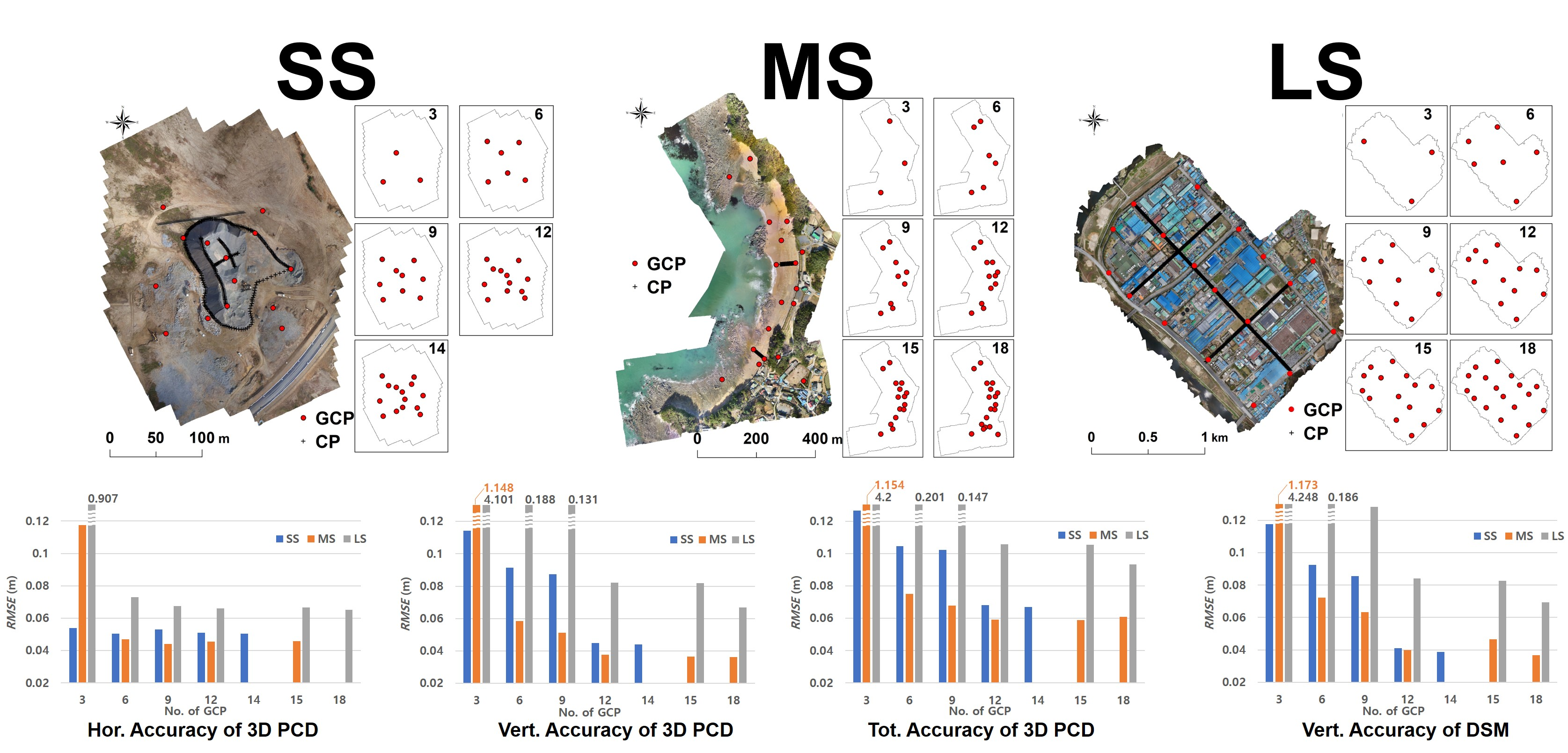
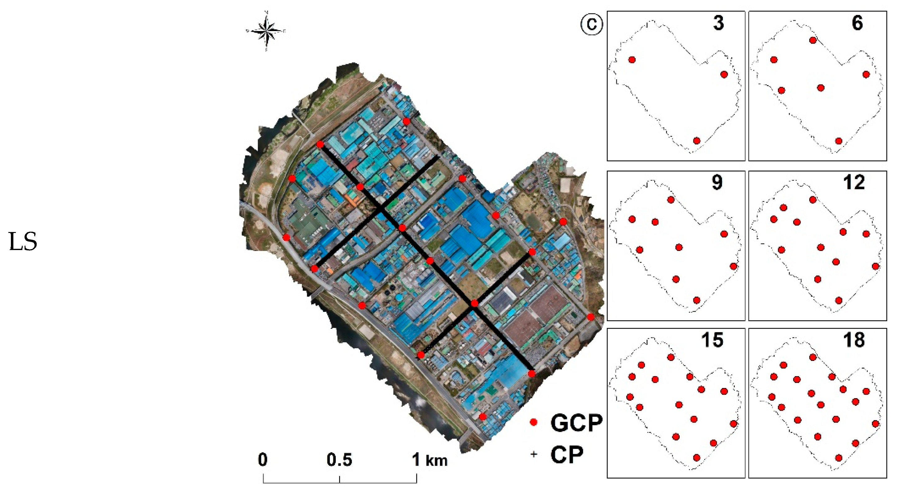
To find the optimal number of GCPs according to each target sites area, the accuracy of the 3D point clouds and DSMs was calculated according to the number of GCPs. GCPs were evenly distributed in each target site so that the GCP network could form a central point polygon capable of covering the site [26,43,54].
Drone modeling has various end-users, and each end-user requires different types of accuracy (vertical, horizontal, or total accuracy) depending on their needs. Therefore, the horizontal, vertical, and total accuracy were calculated individually. Whether this accuracy met the horizontal/vertical accuracy criteria of the American Society for Photogrammetry and Remote Sensing (ASPRS) was assessed [25]. In the Accuracy Quality criteria of ASPRS, the ground sample distance (GSD) of the original image becomes the judgment criterion of accuracy for horizontal accuracy, but the vertical accuracy only distinguishes the absolute accuracy. However, all of the three study sites were non-vegetated terrains. Therefore, non-vegetated in the vertical accuracy class was considered for the judgment of the accuracy (Table 6).

4.1. Horizontal Errors and RMSEs of 3D Point Clouds

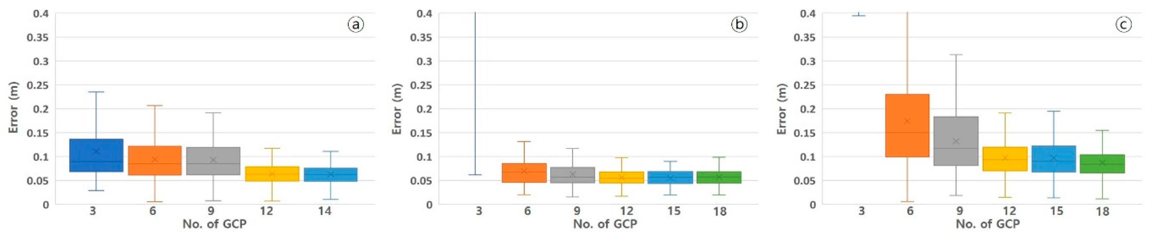
In the SS, the average horizontal errors were 0.05 m for three GCPs and 0.047 m for 14 GCPs. The smallest average horizontal error was 0.046 m when using six GCPs. The standard deviation ranged from 0.019 to 0.020 m, indicating no significant difference between whether the number of GCPs was the largest and the smallest. RMSE also ranged from 0.050 to 0.054 m, corresponding to the range of less than 2 * GSD (5.94 cm) in all cases. In summary, using only three GCPs in the small area of the SS met the horizontal position accuracy criterion of ASPRS. Therefore, using only three GCPs is sufficient when only considering the horizontal accuracy.
The average horizontal error of the MS exceeded 0.1 m when the number of GCPs was three and became smaller when it was six. The error was the smallest (0.041 m) when the number of GCPs was nine. The standard deviation was 0.055 m for three GCPs and sharply decreased from six GCPs with a range of 0.014 to 0.016 m when the number of GCPs was between 6 and 18. RMSE was also inaccurate (approximately 5 * GSD) when three GCPs were used but exhibited an accuracy of less than 2 * GSD (5.38 cm) from six GCPs. As the horizontal accuracy criterion of ASPRS could be met when the number of GCPs was six or larger for the area of the MS, it is necessary to secure at least six GCPs when only the horizontal accuracy is considered.
The accuracy trend of the LS, according to the number of GCPs was very similar to that of the MS. When the number of GCPs was three, the average horizontal error was 0.453 m. However, the error sharply decreased and ranged from 0.061 to 0.067 m when the number of GCPs was between 6 and 18. The standard deviation also decreased from 0.78 m to 0.023–0.028 m when the number of GCPs increased from three. RMSE was also excessively large (close to 1 m) when the number of GCPs was three but decreased to less than 2 * GSD with six GCPs. This indicates that using at least six GCPs can meet the horizontal accuracy criterion of ASPRS for sites whose area is similar to or larger than that of the MS.

4.2. Vertical Errors and RMSEs of 3D Point Clouds

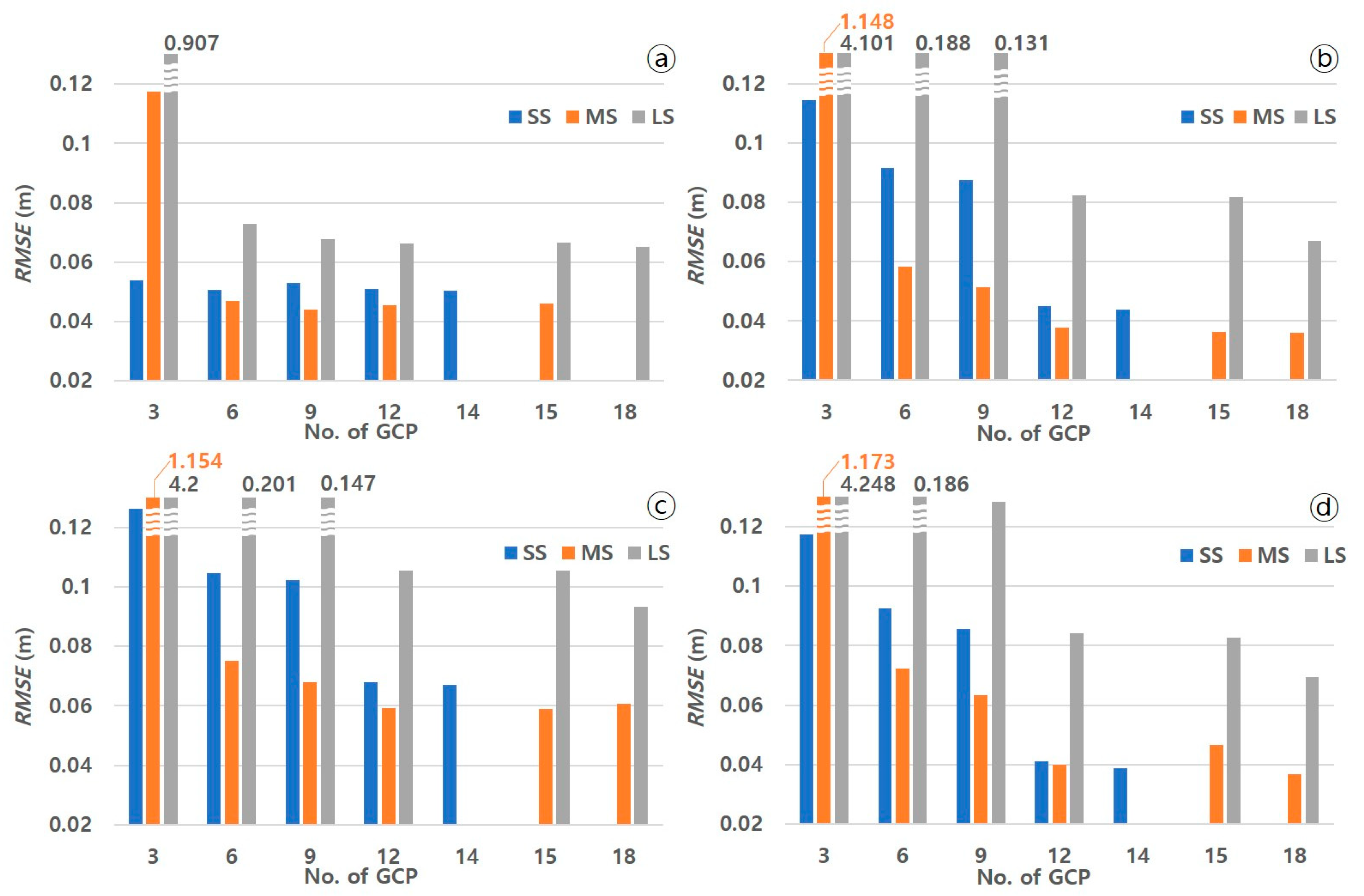
In the SS, the average vertical error was the largest (−0.063 m) when the number of GCPs was three. As the number increased, the error slowly decreased and showed a tendency to converge to zero. The difference between the two cases was only 1 mm when using 12 and 14 GCPs. The standard deviation was also the largest for three GCPs. However, it slowly decreased and there was a small difference when 12 and 14 GCPs were used. RMSE also exceeded 0.1 m for three GCPs but was less than 0.1 m for six and nine GCPs. It was close to 0.04 m from 12 GCPs. These results indicate that at least six GCPs must be installed in small areas, such as SS, considering the vertical accuracy and that at least 12 GCPs must be used to achieve the 5 cm class of ASPRS.
The average vertical error of the MS was very inaccurate (approximately −0.9 m) with three GCPs. As the number increased from 6 to 12, the average vertical error tended to decrease, reaching −0.027 m when it was 12. The error was −0.018 m when 15 and 18 GCPs were used. The standard deviation amounted to 0.7 m when the number of GCPs was three. It was 0.036 m for six GCPs and approximately 0.03 m from nine GCPs. RMSE was 1.148 m for three GCPs and slightly exceeded 0.005 m for six and nine GCPs. It was close to 0.03 m from 12 GCPs. In summary, excellent accuracy could be secured for MS with six GCPs as in SS when considering the vertical position accuracy, the accuracy within 5 cm class was observed when 12 or more GCPs were used.
In the LS, the error was close to 3.8 m with three GCPs, and it exceeded 0.1 m even when the number increased to six. The error was 0.06 m for nine GCPs, and it recorded a stable error range only when the number of GCPs reached 12. The standard deviation also recorded a vast difference when the number of GCPs increased from three to nine but became less than 0.08 m when 12 GCPs were used. The RMSE of the LS became less than 0.1 m from 12 GCPs, unlike the SS and MS, which exhibited excellent accuracy from six GCPs, and the LS exhibiting the highest accuracy using 18 GCPs. In the LS with a large area, the accuracy showed a tendency to improve as the number of GCPs increased. Therefore, higher accuracy could have been achieved through the use of more GCPs. In many cases, however, UAV modeling is not performed in large areas, such as in LS [45].

4.3. Total Errors and RMSEs of 3D Point Clouds

While the horizontal and vertical errors represent xy- and z-direction errors, the total error determines the 3D error in the xyz direction. The mean total errors of the SS were approximately 1 m with three, six, and nine GCPs were used. They significantly decreased to 0.064 and 0.063 m when 12 and 14 GCPs were used. The standard deviation also exhibited the smallest difference when 12 or more GCPs were used. RMSE exceeded 0.1 m for three and six GCPs and presented the best results (0.068 and 0.067 m) when 12 and 14 GCPs were used. Therefore, for the area of the SS, 12 or more GCPs must be used to obtain high accuracy when considering the total accuracy.
In the case of the MS, the average error slightly changed by millimeters from 12 GCPs, which is also true of the standard deviation and RMSE. As RMSE converged to less than 0.06 m from 12 GCPs, it is necessary to install 12 or more GCPs to obtain high accuracy.
In the LS, the average error, standard deviation, and RMSE were significantly reduced when 12 or more GCPs were used as in MS. RMSE was approximately 0.08 m from 12 GCPs. However, the difference in the MS is that the error and standard deviation were somewhat reduced when 18 GCPs were used compared to 12 and 15 GCPs. Thus, 12 or more GCPs must be used to secure high accuracy in large areas, such as LS. If more than 18 GCPs are used, this may increase the accuracy slightly.

4.4. Vertical Errors and RMSEs of DSMs

As DSMs are produced by interpolating 3D point clouds, their accuracy is similar to that of 3D point clouds. In the SS, the average vertical error of DSM was the largest when the number of GCPs was three. It decreased as the number of GCPs increased, and there was almost no difference when 12 and 14 GCPs were used. The standard deviation was also the smallest when using 12 and 14 GCPs similarly to 3D point clouds. Further, RMSE was approximately 0.04 m from 12 GCPs.
In both MS and LS, there was a small difference from the vertical errors of the corresponding 3D point clouds. In summary, in the case of DSM, at least 12 GCPs must be secured to ensure the accuracy of the result in a situation where vertical errors are considered.

4.5. Comprehensive Discussion

For each study site, the number of GCPs to be used to derive highly accurate horizontal, vertical, and total accuracy was different (Table 7). In this table, “minimum” represents the minimum number of GCPs to achieve the accuracy of approximately 0.1 m, which is “excellent” accuracy. Whereas, “optimal” is the number of GCPs required to meet the accuracy of ASPRS. The criteria for vertical and total errors are relative.
This study’s results showed that using only three GCPs could result in the optimal accuracy when considering the horizontal accuracy in a small area. Regarding the vertical and total accuracy in typical drone survey areas, such as SS and MS, 6 GCPs are required for excellent accuracy and 12 GCPs for optimal accuracy. Therefore, installing more than 12 GCPs in an area of approximately 39 ha or less is inefficient.
In the LS, the optimal accuracy was observed from six GCPs when considering the horizontal accuracy. The vertical and total accuracy shown excellent results when at least 12 GCPs were used, and the optimal accuracy was observed using 18 GCPs. In previous studies, the accuracy improved as the number of GCPs increased for very large areas, but the accuracy improvement alongside the increase in the number of GCPs was unknown [19,24,26,43]. In this study, the degree of improvement was not evident, either.
Thus, in typical areas (such as SS and MS), using 12 GCPs will be able to produce highly accurate 3D point clouds and DSMs. In larger areas, the installation of more than 12 GCPs will be required depending on the needs. These results indicate that using too many GCPs may not be effective compared to the labor and cost [55,56], even if the area of the target site is diverse, unlike calculating the optimal number of GCPs per area in previous studies [26,29,41,43].
In order to find methods that can improve UAV modeling accuracy, research has been conducted on solutions, such as camera angle, altitude, overlap, interior orientation parameters of the camera, and calibration, rather than on exterior orientation parameters, such as GCPs. In addition, the need for GCP installation was significantly reduced through the RTK and PPK techniques [25,27,37]. Therefore, with the development of technology, the dependence on the number of GCPs is expected to decrease gradually. Nevertheless, discussion on the number of GCPs will continue, as the method of using GCPs is the most widely used UAV modeling method and the most accurate method.
There are extremely diverse target sites for UAV modeling, as almost all the surface of the earth can be targeted [57,58,59,60,61]. Thus, the elevation and roughness of the ground surface are different. In our study, the three study areas were similar because there was little or no vegetation. However, the main study areas showed variation as follows: (i) Aggregation and bare land (SS), (ii) sand and gravels of beach (MS), and (iii) artificial/man-made areas (LS). In addition, the study on the number of GCPs mentioned in the introduction [38,39,40,41,42,43] also had a difference in elevation of less than 100 m in the study area except for the study of Enoc Sanz-Ablanedo et al. [43]. Generally, the distance between GCPs is referred to as the plane distance, but if the height difference in the study area is large, the height of the study area should be considered because the slant distance increases in proportion to the height difference. If the characteristics of the ground surface are considered in future studies, this may produce interesting results.
Herein, different UAVs and cameras were used for the three study sites. Various models and cameras were used as research materials because UAVs from hobby-type UAVs to industrial UAVs are routinely considered in UAV modeling. Therefore, it will be possible to apply the results of this study more universally. However, in future research, it will be essential to conduct research by reinforcing variable control and changing only the relative area for the same UAV, camera, and site.
Up to 18 GCPs were used for each site. LS exhibited the smallest RMSE with 18 GCPs. In future research, if the set interval for the number of GCPs is reduced to less than 3 and 18 GCPs or more are used, the results can be used to reinforce the results of this study.

5. Conclusions

In this study, the accuracy of 3D point clouds and DSMs were analyzed in three study sites with different areas according to the number of GCPs to propose the optimal number of GCPs for the 3D UAV modeling of various areas.
When the horizontal accuracy was considered, three or more GCPs had to be used in the SS, while six or more GCPs had to be used in the MS and LS. In terms of the vertical accuracy, using only 12 GCPs reached the optimal accuracy in SS and MS, and 18 GCPs in the LS. When considering the total accuracy that covers both the horizontal and vertical accuracy, using only 12 GCPs exhibited the optimal accuracy in SS and MS, and again 18 GCPs in the LS as with the vertical accuracy.
When 3D point clouds, DSMs, and orthomosaics are produced using UAVS, the installation of GCPs requires a lot of time and labor, both indoors and outdoors. Most of the previous studies discussed the number of GCPs in only one study area. On the other hand, our study selected various UAV modelling sites (encompassing natural environment, large industrial complexes, and environmental monitoring areas) based on different areas. We expect that if the results of this study are applied to actual UAV modeling, it may be possible to reduce the time and labor required for GCP installation.

Author Contributions

Conceptualization, J.J.Y.; methodology, J.J.Y.; land survey and UAV operation, J.J.Y., D.W.K.; validation, J.J.Y., S.W.S.; formal analysis, J.J.Y.; investigation, J.J.Y.; resources, S.W.S.; data curation, J.J.Y.; writing—original draft preparation, S.W.S.; writing—review and editing, J.J.Y., E.J.L. and S.W.S.; visualization, J.J.Y., D.W.K.; supervision, J.J.Y., D.W.K., E.J.L. and S.W.S.; project administration, J.J.Y.; funding acquisition, J.J.Y. All authors have read and agreed to the published version of the manuscript.

Funding

This research was funded by Environmental Assessment Monitoring Project (GP-2020-05) of the Korea Environment Institute, and Broadcasting and Communication Development Fund of the Ministry of Science and ICT.

Conflicts of Interest

The authors declare no conflict of interest.

References

  1. Yu, J.J.; Son, S.W.; Park, H.S.; Jeon, H.J.; Yoon, J.H. Evaluation of DSM Accuracy Based on UAS with Respect to Camera Calibration Methods and Application of Interior Orientation Parameters. Korean J. Remote Sens. 2017, 33, 787–798. [Google Scholar]
  2. Kim, D.; Yu, J.J.; Yoon, J.H.; Son, S.W. Analysis of urban surface temperature change during heat wave using UAV thermal infrared camera. J.A.K.G. 2019, 8, 47–60. [Google Scholar]
  3. Burke, C.; Wich, S.; Kusin, K.; McAree, O.; Harrison, M.E.; Ripoll, B.; Ermiasi, Y.; Mulero-Pázmány, M.; Longmore, S. Thermal-Drones as a Safe and Reliable Method for Detecting Subterranean Peat Fires. Drones 2019, 33, 23. [Google Scholar] [CrossRef] [Green Version]
  4. Baltsavias, E.P. Digital ortho-images—A powerful tool for the extraction of spatial-and geo-information. ISPRS J. Photogramm. Remote Sens. 1996, 51, 63–77. [Google Scholar] [CrossRef]
  5. Zhang, L.; Gruen, A. Multi-image matching for DSM generation from IKONOS imagery. ISPRS J. Photogramm Remote Sens. 2006, 60, 195–211. [Google Scholar] [CrossRef]
  6. Quinn, J.D.; Rosser, N.J.; Murphy, W.; Lawrence, J.A. Identifying the behavioural characteristics of clay cliffs using intensive monitoring and geotechnical numerical modelling. Geomorphology 2010, 120, 107–122. [Google Scholar] [CrossRef]
  7. Kasperski, J.; Delacourt, C.; Allemand, P.; Potherat, P.; Jaud, M.; Varrel, E. Application of a terrestrial laser scanner (TLS) to the study of the Séchilienne Landslide (Isère, France). Remote Sens. 2010, 2, 2785–2802. [Google Scholar] [CrossRef] [Green Version]
  8. Fleming, Z.; Pavlis, T. An orientation based correction method for SfM-MVS point clouds—Implications for field geology. J. Struct. Geol. 2018, 113, 76–89. [Google Scholar] [CrossRef]
  9. Mali, V.K.; Kuiry, S.N. Assessing the accuracy of high-resolution topographic data generated using freely available packages based on SfM-MVS approach. Meas. J. Int. Meas. Confed. 2018, 124, 338–350. [Google Scholar] [CrossRef]
  10. Meinen, B.U.; Robinson, D.T. Mapping erosion and deposition in an agricultural landscape: Optimization of UAV image acquisition schemes for SfM-MVS. Remote Sens. Environ. 2020, 239, 111666. [Google Scholar] [CrossRef]
  11. Toutin, T. DSM generation and evaluation from QuickBird stereo imagery with 3D physical modelling. Int. J. Remote Sens. 2004, 25, 5181–5192. [Google Scholar] [CrossRef]
  12. Ishiguro, S.; Yamano, H.; Oguma, H. Evaluation of DSMs generated from multi-temporal aerial photographs using emerging structure from motion–multi-view stereo technology. Geomorphology 2016, 268, 64–71. [Google Scholar] [CrossRef]
  13. Dall’Asta, E.; Forlani, G.; Roncella, R.; Santise, M.; Diotri, F.; Cella, U.d. Unmanned aerial systems and DSM matching for rock glacier monitoring. ISPRS J. Photogramm. Remote Sens. 2017, 127, 102–114. [Google Scholar] [CrossRef]
  14. Yu, J.J.; Kim, D.W.; Yoon, J.H.; Son, S.W. A Study on the Short-term Morphological Beach Changes of Pado-ri Using UAS-based DEM: Focusing on before and after Typhoon Soulik. JAKG 2018, 7, 303–317. [Google Scholar] [CrossRef]
  15. Cardenal, J.; Fernández, T.; Pérez-García, J.L.; Gómez-López, J.M. Measurement of road surface deformation using images captured from UAVs. Remote Sens. 2019, 11, 1507. [Google Scholar] [CrossRef] [Green Version]
  16. Drešček, U.; Kosmatin Fras, M.; Tekavec, J.; Lisec, A. Spatial ETL for 3D Building Modelling Based on Unmanned Aerial Vehicle Data in Semi-Urban Areas. Remote Sens. 2020, 12, 1972. [Google Scholar] [CrossRef]
  17. Son, S.W.; Kim, D.W.; Sung, W.G.; Yu, J.J. Integrating UAV and TLS approaches for environmental management: A case study of a waste stockpile area. Remote Sens. 2020, 12, 1615. [Google Scholar] [CrossRef]
  18. Udin, W.S.; Ahmad, A. Assessment of photogrammetric mapping accuracy based on variation flying altitude using unmanned aerial vehicle. IOP Conf. Ser. Earth Environ. Sci. 2014, 18, 12–27. [Google Scholar] [CrossRef]
  19. Mesas-Carrascosa, F.J.; García, M.D.N.; de Larriva, J.E.M.; García-Ferrer, A. An analysis of the influence of flight parameters in the generation of unmanned aerial vehicle (UAV) orthomosaicks to survey archaeological areas. Sensors 2016, 16, 1838. [Google Scholar] [CrossRef] [Green Version]
  20. Seifert, E.; Seifert, S.; Vogt, H.; Drew, D.; van Aardt, J.; Kunneke, A.; Seifert, T. Influence of drone altitude, image overlap, and optical sensor resolution on multi-view reconstruction of forest images. Remote Sens. 2019, 11, 1252. [Google Scholar] [CrossRef] [Green Version]
  21. Shahbazi, M.; Sohn, G.; Theau, J.; Menard, P. Development and evaluation of a UAV-photo-grammetry system for precise 3D environmental modeling. Sensors 2015, 15, 27493–27524. [Google Scholar] [CrossRef] [PubMed] [Green Version]
  22. Cucci, D.A.; Rehak, M.; Skaloud, J. Bundle adjustment with raw inertial observations in UAV applications. J. Photogramm. 2017, 130, 1–12. [Google Scholar] [CrossRef]
  23. Lee, C.-N.; Oh, J.-H. A study on efficient self-calibration of a non-metric camera for closerange photogrammetry. J. KSGPC 2012, 30, 511–518. [Google Scholar]
  24. James, M.R.; Robson, S.; d’Oleire-Oltmanns, S.; Niethammer, U. Optimising UAV topographic surveys processed with structure-from-motion: Ground control quality, quantity and bundle adjustment. Geomorphology 2017, 280, 51–66. [Google Scholar] [CrossRef] [Green Version]
  25. Kalacska, M.; Lucanus, O.; Arroyo-Mora, J.P.; Laliberté, É.; Elmer, K.; Leblanc, G.; Groves, A. Accuracy of 3D landscape reconstruction without ground control points using different UAS platforms. Drones 2020, 4, 13. [Google Scholar] [CrossRef] [Green Version]
  26. Martínez-Carricondo, P.; Agüera-Vega, F.; Carvajal-Ramírez, F.; Mesas-Carrascosa, F.J.; García-Ferrer, A.; Pérez-Porras, F.J. Assessment of UAV-photogrammetric mapping accuracy based on variation of ground control points. Int. J. Appl. Earth Obs. Geoinf. 2018, 72, 1–10. [Google Scholar] [CrossRef]
  27. Taddia, Y.; Stecchi, F.; Pellegrinelli, A. Coastal mapping using DJI Phantom 4 RTK in post-processing kinematic mode. Drones 2020, 4, 9. [Google Scholar] [CrossRef] [Green Version]
  28. American Society for Photogrammetry and Remote Sensing (ASPRS). ASPRS Positional Accuracy Standards for Digital Geospatial Data (2014); ASPRS: Bethesda, MD, USA, 2015; pp. A1–A26. [Google Scholar]
  29. Son, S.W.; Yoon, J.H.; Jeon, H.J.; Kim, D.W.; Yu, J.J. Optimal flight parameters for unmanned aerial vehicles collecting spatial information for estimating large-scale waste generation. Int. J. Remote Sens. 2019, 40, 8010–8030. [Google Scholar] [CrossRef]
  30. Han, S.-H.; Park, J.-H.; Lee, W.-H. On-site vs. laboratorial implementation of camera self-calibration for UAV photogrammetry. J. KSGPC 2016, 34, 349–356. [Google Scholar] [CrossRef]
  31. Westoby, M.J.; Brasington, J.; Glasser, N.F.; Hambrey, M.J.; Reynolds, J.M. ‘Structure-from-Motion’ photogrammetry: A low-cost, effective tool for geoscience applications. Geomorphology 2012, 179, 300–314. [Google Scholar] [CrossRef] [Green Version]
  32. Anderson, K.; Gaston, K.G. Lightweight unmanned aerial vehicles will revolutionize spatial ecology. Front. Ecol. Environ. 2013, 11, 138–146. [Google Scholar] [CrossRef] [Green Version]
  33. Kršák, B.; Blišťan, P.; Pauliková, A.; Puškárová, P.; Kovanič, Ľ.; Palková, J.; Zelizňaková, V. Use of low-cost UAV photogrammetry to analyze the accuracy of a digital elevation model in a case study. Measurement 2016, 91, 276–287. [Google Scholar] [CrossRef]
  34. Leica Geosystems. Leica Photogrammetry Suite OrthoBASE & OrthoBASE Pro User’s Guide, GIS & Mapping; Leica Geosystems: Atlanta, Georgia, 2003. [Google Scholar]
  35. Turner, I.L.; Harley, M.D.; Drummond, C.D. UAVs for coastal surveying. Coast. Eng. 2016, 114, 19–24. [Google Scholar] [CrossRef]
  36. Forlani, G.; Dall’Asta, E.; Diotri, F.; di Cella, U.M.; Roncella, R.; Santise, M. Quality assessment of DSMs poroduced from UAV flights georeferenced with on-board RTK positioning. Remote Sens. 2018, 10, 311. [Google Scholar] [CrossRef] [Green Version]
  37. Rabaha, M.; Basiouny, M.; Ghanem, E.; Elhadary, A. Using RTK and VRS in direct geo-referencing of the UAV imagery. Nriag. J. Astron. Geophys. 2018, 7, 220–226. [Google Scholar] [CrossRef] [Green Version]
  38. Lim, S.B. Geospatial Information Data Generation Using Unmanned Aerial Photogrammetry and Accuracy Assessment. Ph.D. Thesis, Chungnam National University, DaeJeon, Korea, 2016. [Google Scholar]
  39. Yoo, Y.H.; Choi, J.W.; Choi, S.K.; Jung, S.H. Quality evaluation of orthoimage and DSM based on fixed-wing UAV corresponding to overlap and GCPs. J. Korean Soc. GIS 2016, 24, 3–9. [Google Scholar]
  40. Yun, B.Y.; Sung, S.M. Location accuracy of unmanned aerial photogrammetry results according to change of number of ground control points. J. Korean Assoc. Geogr. Inf. Stud. 2018, 21, 24–33. [Google Scholar]
  41. Coveney, S.; Roberts, K. Lightweight UAV digital elevation models and orthoimagery for environmental applications: Data accuracy evaluation and potential for river flood risk modelling. Int. J. Remote Sens. 2017, 38, 3159–3180. [Google Scholar] [CrossRef] [Green Version]
  42. Agüera-Vega, F.; Carvajal-Ramírez, F.; Martínez-Carricondo, P. Assessment of photogrammetric mapping accuracy based on variation ground control points number using unmanned aerial vehicle. Measurement 2017, 98, 221–227. [Google Scholar] [CrossRef]
  43. Sanz-Ablanedo, E.; Chandler, J.H.; Rodríguez-Pérez, J.R.; Ordóñez, C. Accuracy of unmanned aerial vehicle (UAV) and SfM photogrammetry survey as a function of the number and location of ground control points used. Remote Sens. 2018, 10, 1606. [Google Scholar] [CrossRef] [Green Version]
  44. National Geographic Information Institute (NGII). Public Surveying Regulation Using Unmanned Aerial Vehicles; NGII: Suwon, Korea, 2018.
  45. Manfreda, S.; Dvorak, P.; Mullerova, J.; Herban, S.; Vuono, P.; Justel, J.J.A.; Perks, M. Assessing the accuracy of digital surface models derived from optical imagery acquired with unmanned aerial systems. Drones 2019, 3, 15. [Google Scholar] [CrossRef] [Green Version]
  46. Gaey, C.; Bhardwaj, A. Applications of unmanned aerial vehicles in cryosphere: Latest advances and prospects. Remote Sens. 2020, 12, 948. [Google Scholar]
  47. Rusnák, M.; Sládek, J.; Kidová, A.; Lehotský, M. Template for high-resolution river landscape mapping using UAV technology. Measurement 2018, 115, 139–151. [Google Scholar] [CrossRef]
  48. Shima, T.; Rasmussen, S. UAV Cooperative Decision and Control Challenges and Practical Approaches, 1st ed.; SIAM: Philadelphia, PA, USA, 2008; pp. 15–35. [Google Scholar]
  49. Avellar, G.S.C.; Pereira, G.A.S.; Pimenta, L.C.A.; Iscold, P. Multi-UAV routing for area coverage and remote sensing with minimum time. Sensors 2015, 15, 27783–27803. [Google Scholar] [CrossRef] [PubMed] [Green Version]
  50. Zheng, X.; Wang, F.; Li, Z. A multi-UAV cooperative route planning methodology for 3D fine-resolution building model reconstruction. ISPRS J. Photogramm. Remote Sens. 2018, 146, 483–494. [Google Scholar] [CrossRef]
  51. Snavely, N.; Seitz, S.M.; Szeliski, R. Modeling the world from Internet photo collections. Int. J. Comput. Vis. 2008, 80, 189–210. [Google Scholar] [CrossRef] [Green Version]
  52. Julián, T.; Martin, M.; Šimon, S.; Františrek, C.; Daniel, T. Accuracy of photogrammetric UAV-based point clouds under conditions of partially-open forest canopy. Forest 2017, 8, 151. [Google Scholar]
  53. Gindraux, S.; Boesch, R.; Farinotti, D. Accuracy assessment of digital surface models from unmanned aerial vehicles’ imagery on glaciers. Remote Sens. 2017, 9, 186. [Google Scholar] [CrossRef] [Green Version]
  54. Kim, Y.D.; Park, B.W.; Lee, H.S. Accuracy analysis according to GCP layout type and flying height in orthoimage generation using low-cost UAV. J. Korean Soc. GIS 2018, 26, 31–39. [Google Scholar]
  55. Yang, H.; Li, H.; Gong, Z.; Dai, W.; Lu, S. Relations between the Number of GCPs and Accuracy of UAV Photogrammetry in the Foreshore of the Sandy Beach. J. Coast. Res. 2020, 95, 1372–1376. [Google Scholar] [CrossRef]
  56. Zimmerman, T.; Jansen, K.; Miller, J. Analysis of UAS Flight Altitude and Ground Control Point Parameters on DEM Accuracy along a Complex, Developed Coastline. Remote Sens. 2020, 12, 2305. [Google Scholar] [CrossRef]
  57. Yu, J.J.; Park, H.S.; Yang, Y.J.; Jang, D.H. Assessing the applicability of UAS for detecting geomorphological changes in coastal areas: A case study in the Baramarae Beach in Anmyeon-do. J. Korean Geomorphol. Assoc. 2016, 23, 113–126. [Google Scholar] [CrossRef]
  58. Dąbskia, M.; Zmarz, A.; Pabjanek, P.; Korczak-Abshire, M.; Karsznia, I.; Chwedorzewska, K.J. UAV-based detection and spatial analyses of periglacial landforms on Demay Point (King George Island, South Shetland Islands, Antarctica). Geomorphology 2017, 290, 29–38. [Google Scholar]
  59. De Beni, E.; Cantarero, M.; Messina, A. UAVs for volcano monitoring: A new approach applied on an active lava flow on Mt. Etna (Italy), during the 27 February–02 March 2017 eruption. J. Volcanol. Geotherm. Res. 2019, 369, 250–262. [Google Scholar] [CrossRef]
  60. Nobajas, A.; Waller, R.I.; Robinson, Z.P.; Sangonzalo, R. Too much of a good thing? The role of detailed UAV imagery in characterizing large-scale badland drainage characteristics in South-Eastern Spain. Int. J. Remote Sens. 2017, 38, 2844–2860. [Google Scholar] [CrossRef]
  61. Alexander, C.; Korstjens, A.H.; Hankinson, E.; Usher, G.; Harrison, N.; Nowak, M.G.; Abdullah, A.; Wich, S.A.; Hill, R.A. Locating emergent trees in a tropical rainforest using data from an Unmanned Aerial Vehicle UAV. Int. J. Appl. Earth Obs. 2018, 72, 86–90. [Google Scholar] [CrossRef]
Figure 1. From left to right, a map of the Korean peninsula showing the locations of the three different study sites for (a) the small site, (b) medium site, and (c) large site, aerial orthomosaics of the three labeled study sites, next to images captured of the study sites from UAV.
Drones 04 00049 g001
Figure 2. Flow of research, from in situ operations to the photogrammetry process, for each of the SS, MS, and LS.
Drones 04 00049 g002
Figure 3. Deployment of GCPs (red dots) and CPs (black crosses) for the (a) small site, (b) medium site), and (c) large site.
Drones 04 00049 g003aDrones 04 00049 g003b
Figure 4. 3D point clouds (a) and DSMs (b) of the study sites.
Drones 04 00049 g004
Figure 5. 3D point cloud horizontal error of the study areas: (a) SS, (b) MS, and (c) LS.
Drones 04 00049 g005
Figure 6. 3D point cloud vertical error of the study areas: (a) SS, (b) MS, and (c) LS.
Drones 04 00049 g006
Figure 7. 3D point cloud total error of the study areas: (a) SS, (b) MS, and (c) LS.
Drones 04 00049 g007
Figure 8. Vertical DSM accuracy of the study areas: (a) SS, (b) MS, and (c) LS.
Drones 04 00049 g008
Figure 9. Comprehensive comparison of the RMSE results for the different study sites: (a) horizontal RMSEs of 3D point clouds, (b) vertical RMSEs of 3D point clouds, (c) total RMSEs of 3D point clouds, and (d) vertical RMSEs of DSMs.
Drones 04 00049 g009
Table 1. Summary of study sites, hardware, and specifications used in the research.
Study SiteUAVCameraLand Survey
Small Site, SS: Jiphyeon-ri, Sejong city Area: 7 ha (0.07 km2)Aircraft: DJI Inspire 1 Pro Max speed: 18 m/s Weight: 3.4 kg Flight time: approximately 15 minCamera: DJI X5(FC550) Image size: 4608 * 3456/px Max-Pixels: 16.0M Diagonal FOV: 72 degree Sensor Size: 17.3 × 13.0 mm GNSS: Trimble R8s VRS H: 8 mm + 0.5 ppm RMS VRS V: 15 mm + 0.5 ppm RMS
Medium Site, MS: Pado-ri, Taean-gun Area: 39 ha (0.39 km2)Aircraft: DJI Inspire 1 Pro Max speed: 16 m/s Weight: 1.28 kg Flight time: approximately 23 minCamera: DJI FC300S Image size: 4000 * 3000/px Max-Pixels: 12.76M Diagonal FOV: 94 degree Sensor Size: 6.16 × 4.62 mmGNSS: Huace X90 VRS H: 5 mm + 1 ppm RMS VRS V: 10 mm + 2 ppm RMS
Large Site, LS: Daedeok industrial complex, Daejeon metropolitan city Area: 342 ha (3.42 km2)Aircraft: QuestUAV DataHawk (Fixed wing) Max speed: 25 m/s Weight: 2 kg Flight time: approximately 45 minCamera: SONY ILCE-QX1 Image size: 5456 * 3632/px Max-Pixels: 20M Diagonal FOV: 73.7 degree Sensor Size: 23.2 × 15.4 mmGNSS: Trimble R8s VRS H: 8 mm + 0.5 ppm RMS VRS V: 15 mm + 0.5 ppm RMS
Table 2. Software used in the research.
Automatic Mission Flight3D Modeling ProcessAccuracy Analysis and Mapping
Pix4d CaptureAgisoft Metashape (v.1.5.3)CloudCompare (v.2.10.2) and ArcMap (v.10.1)
Table 3. Results of UAV flight and field survey.
Study SiteFlight Plan and ParametersGNSS Survey
SSFlight time: 10 m Flight mission: 1 Flight altitude: 120 mImages: 52 Front overlap: 85% Side overlap: 65%No. of GCPs: 14 (5 cases: 3, 6, 9, 12, 14) No. of CPs: 311
MSFlight time: 15 m/mission Flight missions: 4 Flight altitude: 70 mImages: 1022 Front overlap: 80% Side overlap: 80%No. of GCPs: 18 (6 cases: 3, 6, 9, 12, 15, 18) No. of CPs: 79
LSFlight time: 40 m/mission Flight missions: 3 Flight altitude: 150 mImages: 1163 Front overlap: 80% Side overlap: 80%No. of GCPs: 18 (6 cases: 3, 6, 9, 12, 15, 18) No. of CPs: 436
Table 4. Results of the field survey, summarizing the average number of points, density, and resolution of the 3–18 GCP results.
Study SiteAvg. Number of PointsAvg. Point Density (points/m2)Avg. Resolution of DSM (cm/px)Avg. Resolution of Orthomosaic (cm/px)
SS5,525,04770.711.92.97
MS53,859,77386.410.82.69
LS207,286,23542.515.33.84
Table 5. RMSEs of the 3D point clouds (in meters).
RMSESiteNo. of GCPs
36912141518
3D point cloudHorizontalSS0.0540.0500.0530.0510.050n/an/a
MS0.1170.0460.0440.045n/a0.0450.048
LS0.9070.0720.0680.066n/a0.0670.065
VerticalSS0.1140.0920.0870.0450.044n/an/a
MS1.1480.0580.0510.038n/a0.0360.036
LS4.1010.1880.1310.082n/a0.0820.067
TotalSS0.1260.1040.1020.0680.067n/an/a
MS1.1540.0750.0670.059n/a0.0580.060
LS4.2000.2010.1470.105n/a0.1050.093
DSMVerticalSS0.1170.0920.0850.0410.039n/an/a
MS1.1730.0720.0630.040n/a0.0460.037
LS4.2480.1860.1280.084n/a0.0830.069
Table 6. Horizontal accuracy quality examples for high-accuracy digital planimetric data and vertical accuracy quality examples for digital elevation data.
Horizontal Accuracy Class RMSEx, and RMSEy (cm)RMSExy (cm)Approximate GSD of Source Imagery (cm) Vertical Accuracy Class (cm) Absolute Accuracy: RMSEz Non-Vegetated (cm)
0.630.90.31–0.631 cm1.0
1.251.80.63–1.252.5 cm2.5
2.53.51.25–2.55 cm5.0
5.07.12.5–5.010 cm10.0
Table 7. Minimum and optimal number of GCPs for each area and accuracy (horizontal, vertical, and total).
HorizontalVerticalTotal
3D Point Cloud3D Point CloudDSM3D Point Cloud
MinimumOptimalMinimumOptimalMinimumOptimalMinimumOptimal
SS (7 ha)3>36>126>126>12
MS (39 ha)6>66>126>126>12
LS (342 ha)6>612>1812>1812>18

