On the Self-Calibration of Aerodynamic Coefficients in Vehicle Dynamic Model-Based Navigation

Abstract

The performance of vehicle dynamic model (VDM)-based navigation largely depends on the accurate determination of aerodynamic coefficients that are unknown a priori. Among different techniques, such as model simulations or experimental analysis in a wind tunnel, the method of self-calibration via state-space augmentation benefiting Global Navigation Satellite System (GNSS) positioning represents an interesting and economical alternative. We study this technique under simulation with the goal of determining the impact of aircraft maneuvers on the precision and (de)-correlation of the aerodynamic coefficients among themselves and with respect to other error-states. A combination of different maneuvers indicates to be essential for obtaining satisfactory aerodynamic coefficients estimation and reduce their uncertainty.

The expansion of applications utilizing small unmanned aerial vehicles (UAVs) in the last few years is unprecedented. No aviation sector has experienced such rapid technological evolution in both hardware and software. However, most light-weight UAVs made for large zone inspections and mapping rely on GNSS positioning as the main element that assures the drone navigation along a pre-programmed path and, thus, its safety. As the average satellite signal power at reception is very weak, −125 dbm [1] (−75 dbm for WiFi [2]), its reception can be relatively easily perturbed either unintentionally (due to an interference) or intentionally (via jamming or spoofing). In the absence of GNSS signal, the UAV executes a safe-fail procedure that generally relies on autonomous sensors. Over a time interval longer than a minute, its performance is usually sufficient only for controlling vehicle attitude and altitude.

In this context, a certain form of vehicle dynamic model (VDM)-based navigation [3,4] has shown a considerably better performance in comparison to the traditional inertial-based counterpart in GNSS-denied environment for fixed-wing UAV [5]. This technique is potentially promising also for improving the accuracy of sensor orientation for mapping within the nominal scenario with GNSS signal reception [6]. However, in contract to INS/GNSS integration, the VDM-based navigation is a vehicle-dependent technique. In other words, its implementation requires to determine the a-prior unknown aerodynamic coefficients reflecting the physical properties of a particular aircraft. Only with “reasonably” correct coefficients, the dynamic process model will represent the realistic flight behavior of the platform so the navigation filter works correctly, otherwise it may become unstable and diverge [7].

The determination of some model parameters is straightforwards as the aircraft weight or the wing surface. Wind tunnel tests or Computational Fluid Dynamic (CDF) simulations can be conducted to accurately determine some other VDM parameters. However, a more practical option is to determine their values directly in-flight when GNSS signals are present [3].

In either case, it is difficult to estimate the parameter individually because of their implicit correlation with each other [3]. The limitations of in-flight estimation of VDM parameters during normal dynamics advocate investigating a dedicated calibration procedure that lower the uncertainty of their estimation as compared to nominal mission dynamic while reducing the remaining correlations.

This study investigates this option by simulating VDM parameter calibration through different aircraft maneuvers with sensory and external perturbations in a Monte-Carlo manner. The rest of the paper is organized, as follows: Section 1 synthesizes the principle of VDM-based navigation, Section 2 provides details of different simulation steps and considered scenarios, Section 3 analyses the simulation outcomes, and Section 4 summarizes the findings.

1. Vehicle Dynamic Model

While the essentials of VDM-based navigation system is presented here shortly, more technicalities of the derivations can be found in [3] and details on the employed dynamic model can be found in [8].

1.1. Frames Definition

Within the context of navigation, the following five reference frames are considered: the inertial (i)-frame is an Earth Centered Inertial (ECI) frame, the Earth (i)-frame is an Earth Centered Earth Fixed (ECEF) frame, the local-level (l)-frame is oriented in north, east, and down directions with respect to the tangent plane on a reference ellipsoid [9]. Definitions of body (b)-frame and wind (w)-frame with respect to l-frame can be perceived from Figure 1.

The wind frame has its first axis in direction of airspeed $\mathbf{V}$, and is defined by two angles with respect to body frame, angle of attack $\alpha$ and sideslip angle $\beta$. The velocity of airflow that is due to UAV’s velocity with respect to ground $\mathbf{v}$ and wind velocity $\mathbf{w}$ is denoted by airspeed vector $\mathbf{V}$ as

$$\mathbf{V}=\mathbf{v}-\mathbf{w}.$$

(1)

The rotation matrix ${\mathbf{C}}_b^w$ from body frame to wind frame is defined as a function of angle of attack $\alpha$ and sideslip angle $\beta$ as

$${\mathbf{C}}_b^w={\mathbf{R}}_3\left(\beta \right){\mathbf{R}}_2\left(\alpha \right),$$

(2)

where ${\mathbf{R}}_i$ denotes the elementary rotation matrix around the i-th axis.

1.2. Motion States

We consider modeling rigid body in arbitrary three-dimensional (3D) space affected by Earth gravity via specific forces $\mathit{f}$, and moments $\mathit{M}$, as in [5]. This is described via a set of first-order differential Equations (4)–(7) considering Earth rotation, curvature, and normal gravity, the resolution of which provides the “navigation states”

$${\mathit{X}}_n={\left[{{\mathit{r}}_e^l}^T,{{\mathit{v}}_e^l}^T,{{\mathit{q}}_b^l}^T,{{\mathit{\omega }}_{ib}^b}^T\right]}^T$$

(3)

where the position vector ${\mathit{r}}_e^l={[\varphi ,\lambda ,h]}^T$ represents position of platform (represented by the origin of body frame) in Earth frame and in ellipsoidal coordinates, the velocity vector ${\mathit{v}}_e^l={[v_N,v_E,v_D]}^T$ represents velocity of platform, as observed in Earth frame and expressed in local (NED) frame, the quaternion ${\mathit{q}}_b^l={[q_0,q_1,q_2,q_3]}^T$ represents orientation of body frame (platform) with respect to local frame and the angular velocity vector ${\mathit{\omega }}_{ib}^b={[{\omega }_x,{\omega }_y,{\omega }_z]}^T$ represents angular velocity (rotation rate) of body frame with respect to inertial frame, expressed in body frame. The ⊗ operator defines quaternion cross-products, as defined in [10].

This set of equations can be expressed as

$$\begin{array}{cc}\hfill & {\dot{\mathit{r}}}_e^l=D^{-1}{\mathit{v}}_e^l\hfill \end{array}$$

(4)

$$\begin{array}{cc}\hfill & {\dot{\mathit{v}}}_e^l=C_b^l{\mathit{f}}^b+{\mathit{g}}^l-({\mathsf{\Omega }}_{el}^l+2{\mathsf{\Omega }}_{ie}^l){\mathit{v}}_e^l\hfill \end{array}$$

(5)

$$\begin{array}{cc}\hfill & {\dot{\mathit{q}}}_b^l=\frac{1}{2}{\mathit{q}}_b^l\otimes {\left[{\mathit{\omega }}_{lb}^b\right]}_q\hfill \end{array}$$

(6)

$$\begin{array}{cc}\hfill & {\dot{\mathit{\omega }}}_{ib}^b={\left(I^b\right)}^{-1}\left[{\mathit{M}}^b-{\mathsf{\Omega }}_{ib}^b\left(I^b{\mathit{\omega }}_{ib}^b\right)\right],\hfill \end{array}$$

(7)

where any ${\mathbf{\Omega }}_{pq}^r$ is a skew-symmetric matrix representation of associated vector.

In Equation (4), $D^{-1}$ matrix is a function of ellipsoid curvatures, height and longitude. In Equation (5), the rotation matrix $C_b^l$ can be expressed as a known function of the quaternion ${\mathit{q}}_b^l$. In (6), ${\mathit{\omega }}_{lb}^b$ is calculated as

$${\mathit{\omega }}_{lb}^b={\mathit{\omega }}_{ib}^b-{\left(C_b^l\right)}^T\left({\mathit{\omega }}_{ie}^l+{\mathit{\omega }}_{el}^l\right),$$

(8)

1.3. Dynamic Model

The dynamic model for a particular vehicle, a fixed-wing UAV for example, describes how $\mathit{f}$ and $\mathit{M}$ are specified following an aerodynamic model. This model takes motion states, wind velocity, actuators, and physical parameters of the platform as inputs. The models vary for different UAV types. A fixed-wing platform is considered here, as described in [3]. As depicted schematically in Figure 1, this UAV has a single propeller, with aileron, elevator, and rudder control surfaces. The models for aerodynamic forces and moments for this UAV are borrowed from [8].

Four components of aerodynamic forces and three components of aerodynamic moments are recognizable in this model: thrust, drag, lateral, and lift forces ($F_T$, $F_x^w$, $F_y^w$, and $F_z^w$, respectively), as well as roll, pitch, and yaw moments ($M_x^b$, $M_y^b$, and $M_z^b$, respectively). All moment components and thrust force (along $x_b$-axis) are expressed in body frame, while lift, lateral, and drag forces are expressed in wind frame, as follows:

$$\begin{array}{cc}\hfill F_T& =\rho n^2{D}^4\left(C_{F_{T}1}+C_{F_{T}2}J+C_{F_{T}3}{J}^2\right)\hfill \end{array}$$

(9)

$$\begin{array}{cc}\hfill F_x^w& =\overline{q}S\left(C_{F_{x}1}+C_{F_x\alpha }\alpha +C_{F_x\alpha 2}{\alpha }^2+C_{F_x\beta 2}{\beta }^2\right)\hfill \end{array}$$

(10)

$$\begin{array}{cc}\hfill F_y^w& =\overline{q}S\left(C_{F_{y}1}\beta \right)\hfill \end{array}$$

(11)

$$\begin{array}{cc}\hfill F_z^w& =\overline{q}S\left(C_{F_{z}1}+C_{F_z\alpha }\alpha \right)\hfill \end{array}$$

(12)

$$\begin{array}{cc}\hfill M_x^b& =\overline{q}Sb\left(C_{M_{x}a}{\delta }_a+C_{M_x\beta }\beta +C_{M_x{\tilde{\omega }}_x}{\tilde{\omega }}_x+C_{M_x{\tilde{\omega }}_z}{\tilde{\omega }}_z\right)\hfill \end{array}$$

(13)

$$\begin{array}{cc}\hfill M_y^b& =\overline{q}S\overline{c}\left(C_{M_{y}1}+C_{M_{y}e}{\delta }_e+C_{M_y{\tilde{\omega }}_y}{\tilde{\omega }}_y+C_{M_y\alpha }\alpha \right)\hfill \end{array}$$

(14)

$$\begin{array}{cc}\hfill M_z^b& =\overline{q}Sb\left(C_{M_z{\delta }_r}{\delta }_r+C_{M_z{\tilde{\omega }}_z}{\tilde{\omega }}_z+C_{M_z\beta }\beta \right)\hfill \end{array}$$

(15)

where $\rho$ is air density, n is propeller speed, D is propeller diameter, $\overline{q}$ is dynamic pressure defined as $\frac{\rho V^2}{2}$, S is wing surface, b is wingspan, $\overline{c}$ is mean aerodynamic chord, $J=V/\left(D\pi n\right)$, ${\tilde{\omega }}_x=b{\omega }_x/\left(2V\right)$, ${\tilde{\omega }}_y=\overline{c}{\omega }_y/\left(2V\right)$, ${\tilde{\omega }}_z=b{\omega }_z/\left(2V\right)$, and $C_{\dots }$’s are aerodynamic coefficients for the particular UAV at hand. Deflections of aileron, elevator, and rudder are denoted by ${\delta }_a$, ${\delta }_e$, and ${\delta }_r$, respectively.

The specific force vector

$$\begin{array}{c}\hfill {\mathit{f}}^{\mathit{b}}=\frac{1}{m}\left(\begin{array}{c}{\left[\begin{array}{ccc}{F}_T& 0& 0\end{array}\right]}^T+C_w^b{\left[\begin{array}{ccc}{F}_x^w& F_y^w& F_z^w\end{array}\right]}^T\end{array}\right)\end{array}$$

(16)

is composed of these four components divided by the mass of the UAV, and the moments vector

$$\begin{array}{c}\hfill {\mathit{M}}^{\mathit{b}}={\left[\begin{array}{ccc}{M}_x^b& M_y^b& M_z^b\end{array}\right]}^T\end{array}$$

(17)

is composed of these three components. Equations (4)–(7), together with (9)–(17) form the VDM for the sample fixed-wing UAV.

1.4. Estimation Scheme

The navigation system utilizes VDM as main process model within a differential filter, along with other necessary models for augmented states. An Extended Kalman filter (EKF) [11] is chosen to estimate corrections to the states ($\delta \mathit{X}$) and associated covariance matrix (P). Other types of filters/estimators, such as unscented Kalman filter (UKF), could also be used. EKF utilizes a linearized version of process model (via $F=\partial \dot{\mathit{X}}/\partial \mathit{X}$, with $\mathit{X}$ being the state vector) and a linearized version of observation model (via $H=\partial \mathit{Z}/\partial \mathit{X}$, with $\mathit{Z}$ being the observation vector) to perform prediction on covariance matrix P and update on both state vector $\mathit{X}$ and covariance matrix. Prediction on states is done via a nonlinear process model, i.e., via Equations (4)–(17).

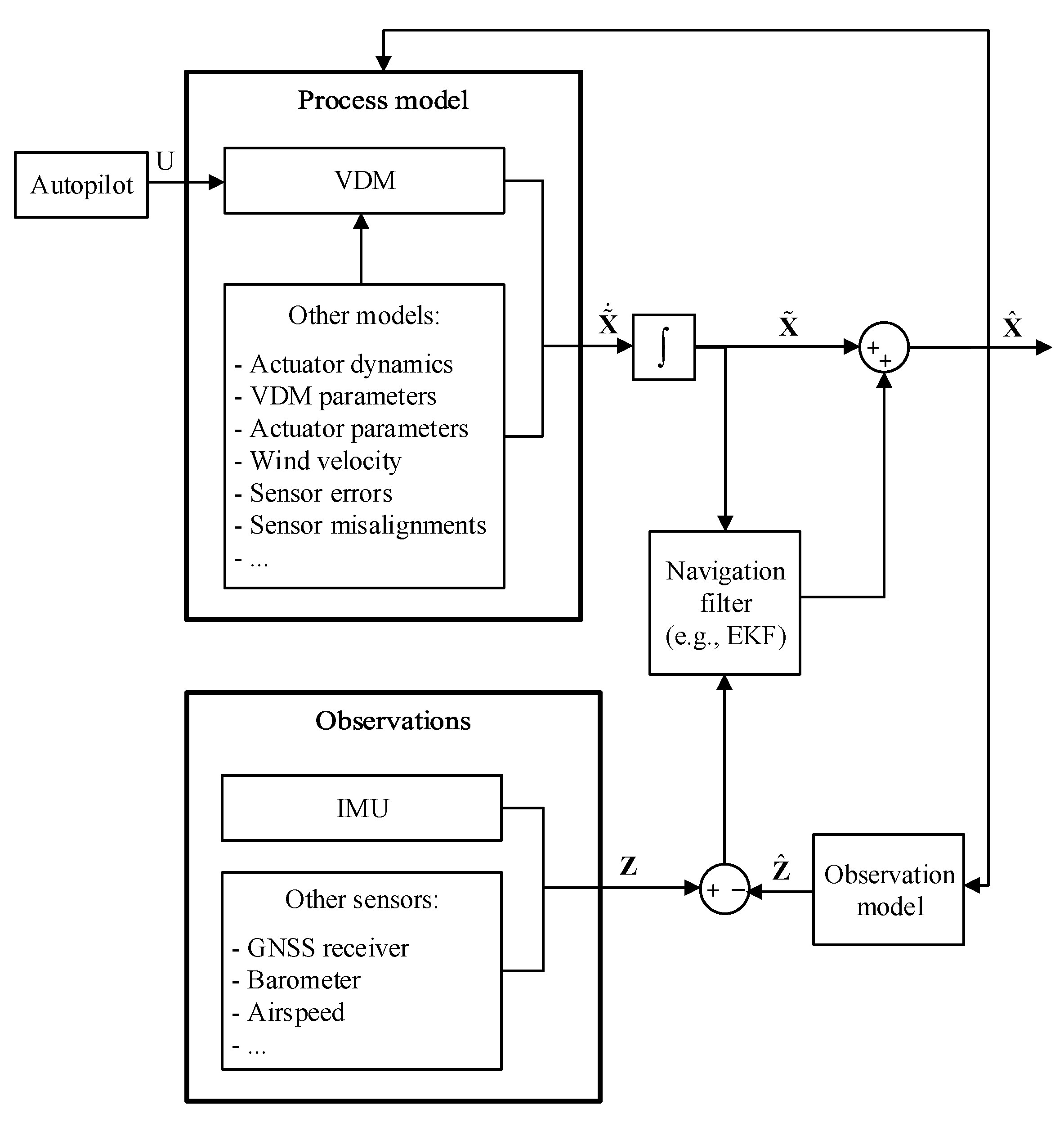
As depicted in Figure 2, VDM provides the navigation solution (${\mathit{X}}_n$, not shown in Figure 2), as part of the augmented states vector ($\mathit{X}$), which is updated by the filter based on available observations. Hence, IMU data are treated as observations, just the way data from other sensors such as GNSS receiver, barometer, and airspeed sensor are when available. It is important to note that IMU observations are related to system states via the VDM. Any other available sensor, such as optic flow sensor and magnetometer, can also be integrated within the navigation system as additional observation sources. Nevertheless, only GNSS and IMU data are used for the simulated scenarios in this study and they are part of the observations vector $\mathit{Z}$ in Figure 2.

The VDM needs to be fed with actuator states. If internal dynamics of the actuators is ignored, actuator states will be equivalent to the control input ($\mathit{U}$). Otherwise, the control input is fed to associated models for actuator dynamics, which provide actuator states to the VDM. The parameters of actuator dynamics model may also be part of the augmented state that is estimated within the filter. Another needed input for the VDM is the wind velocity (${\mathit{X}}_w$, “Other models” block, not shown in Figure 2), which is estimated within the navigation system with or without the aid of airspeed sensor(s). Reliable airspeed data is expected to improve the redundancy and possibly the accuracy of wind estimation.

Finally, the parameters of VDM, which represents the physical properties of the UAV, are required. Pre-calibration of these parameters and their application as fixed-known values is an option. However, to increase the flexibility and accuracy of the proposed approach while minimizing the effort in calibration (e.g., in a wind tunnel), in-flight estimation/refinement of VDM parameters (${\mathit{X}}_p$) is proposed as an augmented state ${\mathit{X}}_p={\left[\begin{array}{c}S,\overline{c},b,D,C_{F_i},C_{M_j},{\tau }_n\end{array}\right]}^T$, where i = 1:10 and j = 1:11 correspond to the coefficients, in order of appearance, related to forces and moment in Equations (9)–(12) and Equations (13)–(15), respectively.

Last but not least, time-correlated IMU errors (${\mathit{X}}_e$) are also modeled and estimated within the navigation system. For this implementation, the states (${\mathit{X}}_e$) will only be composed with accelerometer and gyroscope bias for each axis:

$${\mathit{X}}_e={\left[b_{A_x},b_{A_y},b_{A_z},b_{G_x},b_{G_y},b_{G_z}\right]}^T$$

(18)

For this work, the system states vector is therefore:

$$\mathit{X}={\left[{\mathit{X}}_n,{\mathit{X}}_p,{\mathit{X}}_e,{\mathit{X}}_w\right]}^T$$

(19)

The continuous states derived by the models $\dot{\tilde{\mathit{X}}}$ are integrated to obtain the system state further used in an estimator, here an EKF. The predicated state $\tilde{\mathit{X}}$ is combined with observations from the different sensors $\mathit{Z}$ to update and obtain the state $\widehat{\mathit{X}}$ depicted in Figure 2. The different observation models $\widehat{\mathit{Z}}$ can thus correct the sensor measurements thanks to additional models (“Other models”).

2. Simulation Setup

In the following parts, we first present the methodology of the calibration procedure. Afterwards, we assess the quality of the VDM parameter determination with respect to (a) parameter error, (b) its predicted incertitude, and (c) correlation to other parameters. Finally, we discuss a combination of maneuvers for an “optimal” in-flight calibration procedure.

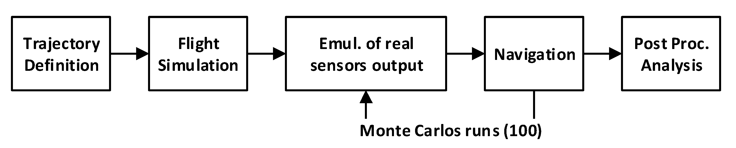
Figure 3 depicts the steps of the calibration methodology. As the condition of calibration can be chosen we assume that GNSS observations are available and we suppose the wind to be zero or negligible. Thus, the wind is not estimated in the navigation solution. The reasoning is to isolate the influence of the trajectory dynamic into the coefficients determination without adding extra parameters (Wind, three components) to be estimated.

2.1. Trajectory Definition

Some aspects considered in the trajectory definition are execution time, the feasibility of maneuvers for the autopilot, and/or the drone operator and continuity of GNSS signal tracking. Therefore, the designed trajectories last less than five minutes and avoid steep turns and attitude changes that could lead to a loss of GNSS signal reception.

Seven trajectory-segments are defined and separated into three categories. These are: straight line, circular orbit (loiter), and “figure-eight” or “infinite” loop. The last trajectory is a combination of different maneuvers. A straight line is characterized by two waypoints defining its start and end. The actual path is not a straight line per-say because the autopilot tries to reach the waypoints by compensations of different actuators. The resulting behavior depends on a particular control parameters, but generally resembles some oscillations around the straight segment, as presented on the first raw in

Table 1. Categorization of considered trajectories (and combinations) into seven types.

Straight Line	Level		Level Descending		Level Ascending
Orbit	Controlled			Auto pilot
Infinity Loop	Level			Descending/Ascending

.

Two categories of orbit/loiters are considered, as shown in the second raw in Table 1: manual and autopilot controlled. The former is performed by setting the control surfaces to a constant value, while the latter is executed by autopilot guidance following waypoints distributed along a circle. The infinity loop concatenates two complete orbits controlled with the autopilot in the opposite direction, with or without forced changes in altitude. These two segments are presented at the bottom of Table 1. The last trajectory type is a concatenation of the above-mentioned segments with the addition of velocity changes. The user defined waypoints are represented in pink crosses on the different figures and the axes ($xE$, $xN$, and $xU$) belong to a local-level frame in East-North-Up orientation (ENU).

2.2. Flight Simulation

Once the trajectory shape is defined, the corresponding dynamics follows from the guidance and control acting on a particular platform. The implementation here is inspired from the model that is presented in [8] while considering small fixed-wing aircraft described in [5].

The VDM-based navigation stemming from aerodynamic model can only be performed during in-flight conditions, i.e., after takeoff and prior touch-down. Practically, this can be achieved by transferring the navigation states from inertial-based navigation after take-off. Within the simulation, the platform is initialized airborne with chosen heading and velocity at the first waypoint. The guidance uses waypoints coordinates expressed in a local-level frame relative to the first waypoint together with a desired velocity and attitude of the platform at each of them.

The waypoints are considered to be reached (cleared) when the platform is within a radius of 15 m, then the next waypoint is activated. The guidance dictates the action of actuators to be taken directing the plane to the next waypoint. The controller generates the actuator states (i.e, the elevator, aileron and ruder angles, and propeller speed) and together with ideal VDM parameters, they define the nominal forces and moments following the model described in Section 1. The ideal-reference trajectory follows from rigid-body motion. Simultaneously, the ideal sensors output is generated at a desired frequency, i.e., in Equations (16) and (17) for the IMU and from the derived states ${\mathit{r}}_e^l$ as presented in Equation (3) for GNSS. parentheses The ideal trajectory is saved as a reference, whereas the generated sensors and actuator commands are used in the following step. The generated control commands are delay-free, implying the absence of time stamping errors in the data or delay of actuators when reaching the desired state. The influence of time-delay errors has been investigated in [12].

2.3. Sensor and VDM Parameter Errors

At this stage, the software possesses all of the information to simulate the behavior of a platform following a defined trajectory and, most importantly, the sensors and actuator outputs at each discrete step. The ideal sensors readings (accelerometers, gyroscopes) are first corrupted with errors such as random bias, 1st order Gauss–Markov process and white noise. The considered error characteristics are summarized in

Table 2. Noise errors added to the sensor data.

Error Type	Notation	Value	[Units]
Gyro. bias	$b_G$	720	[deg/h]
Gyro. correlated noise	${\sigma }_{G_{GM1}^{PSD}}$	0.0028	[deg/s/$\sqrt{Hz}$]
	$1/{\beta }_G$	200	[s]
Gyro. white noise	${\sigma }_{G_{WN}^{PSD}}$	0.18	[deg/$\sqrt{Hz}$]
Acc. bias	$b_A$	8	[mg]
Acc. correlated noise	${\sigma }_{A_{GM1}^{PSD}}$	0.05	[mg]
	$1/{\beta }_A$	200	[s]
Acc. white noise	${\sigma }_{A_{WN}^{PSD}}$	50	[mg/$\sqrt{Hz}$]
GNSS white noise (each direction)	${\sigma }_{GNSS}$	1	[m]

. Their values correspond to a small MEMS-IMU [13] that was employed in an experimental scenario [5] with noise characteristics analyzed in [14]. The considered GNSS observations corresponds to single-point-positioning.

In the simulation environment, no residual imperfections are considered to be related to the knowledge of sensor position and alignment with respect to body frame.

The initial uncertainties for the VDM parameters ${\mathit{X}}_p$ are fixed to 20 percent of their reference values (1$\sigma$). Such uncertainty is reflected in the initial covariance matrix, while 100 runs of Monte-Carlo are simulated for each trajectory to diversify the initial error in parameter values. Similarly, the realization of stochastic processes in the simulated sensors (IMU, GNSS) is part of Monte-Carlo simulations. The choice for 100 runs was revealed to be sufficient to qualitatively capture the stochastic distribution among the different runs. This number could be increased to have a better quantitative perception about the errors. The initial uncertainties for the navigation states ${\mathit{X}}_n$ correspond to the simulated sensor quality and are summarized in

Table 3. Initial navigation state uncertainties.

Navigation States		Values	Units
Position	- all axis	1	[m]
Velocity	- horizontal	1	[m]
	- vertical	0.5	[m]
Attitude	- roll/pitch	3	[deg]
	- yaw	5	[deg]
Angular rate	- all axis	1	[deg/s]

.

In the simulation environment, the guidance and control is considered to be independent from the navigation. In other-words, the guidance is based on “error-free” sensors and VDM-parameters, reason for which the realized trajectory for each simulation may differ more from the ideal-desired trajectory. However, this fact is less important to examine the parameter estimation evolution with respect to real model values.

3. Analysis and Discussion

The main subject of these investigations is to observe how flight dynamic influences the estimation quality of VDM-parameters (aerodynamic coefficients). Such quality can be analyzed in terms of (i) the remaining parameter errors and the reduction of the estimated parameter uncertainty and (ii) the residual correlations among the parameters among themselves and with respect to other states. The outcome of such analysis is presented in the following sections.

3.1. Parameter Estimation

As already mentioned, a higher dynamic helps the estimation of the VDM parameters. It excites different groups of parameters and improve their estimation by (i) decreasing the variance and (ii) by decreasing their dependence on auxiliary states.

Table 4. Group of VDM parameter error per trajectory [in %] at the end of a maneuver.

Trajectory	per VDM Category (Lowest to Largest)			Total
Descend. Straight L.	$F_y:$ 15.3%	$<M_y<M_z<F_T<F_x<F_z<$	$M_x:$ 26.4%	18.4%
Straight line	$M_y:$ 10.0%	$<F_y<F_T<F_z<M_x<M_z<$	$F_x:$ 17.6%	13.8%
Climbing Straight L.	$M_y:$ 9.1%	$<F_y<F_T<F_z<M_x<M_z<$	$F_x:$ 17.4%	13.7%
Controlled Orbit	$M_y:$ 11.2%	$<F_y<M_z<M_x<F_z<F_x<$	$F_T:$ 20.0%	13.5%
Orbit w. AutoPilot	$M_y:$ 10.8%	$<F_y<M_x<M_z<F_z<F_x<$	$F_T:$ 17.9%	13.2%
8 Loop w. Alt. fix	$M_z:$ 8.3%	$<M_x<F_y<M_y<F_z<F_x<$	$F_T:$ 17.5%	11.1%
8 Loop w. Alt. var.	$M_z:$ 8.3%	$<M_x<M_y<F_y<F_z<F_x<$	$F_T:$ 16.8%	10.9%

accentuates this fact by showing the % of remaining error in groups of VDM parameters after different type of maneuvers.

The different groups are: thrust force $F_T$, forces along x, y, and z body axis given by $F_x$, $F_y$, and $F_z$, respectively, and the three moments $M_x$, $M_y$, and $M_x$ around the three body axis. These have been defined from Equations (9)–(15).

It is easily identifiable that better estimation is achieved with more complex trajectories, but that each maneuver-type influences different (groups of) coefficients. Hence, a sequence of maneuvers is needed for in-flight parameter calibration. Additionally, the lack of velocity changes in the suggested trajectories explains the relatively poor estimation of the thrust force group ($F_T$). Therefore, velocity variations should be considered during each maneuver.

3.2. Parameter Correlation

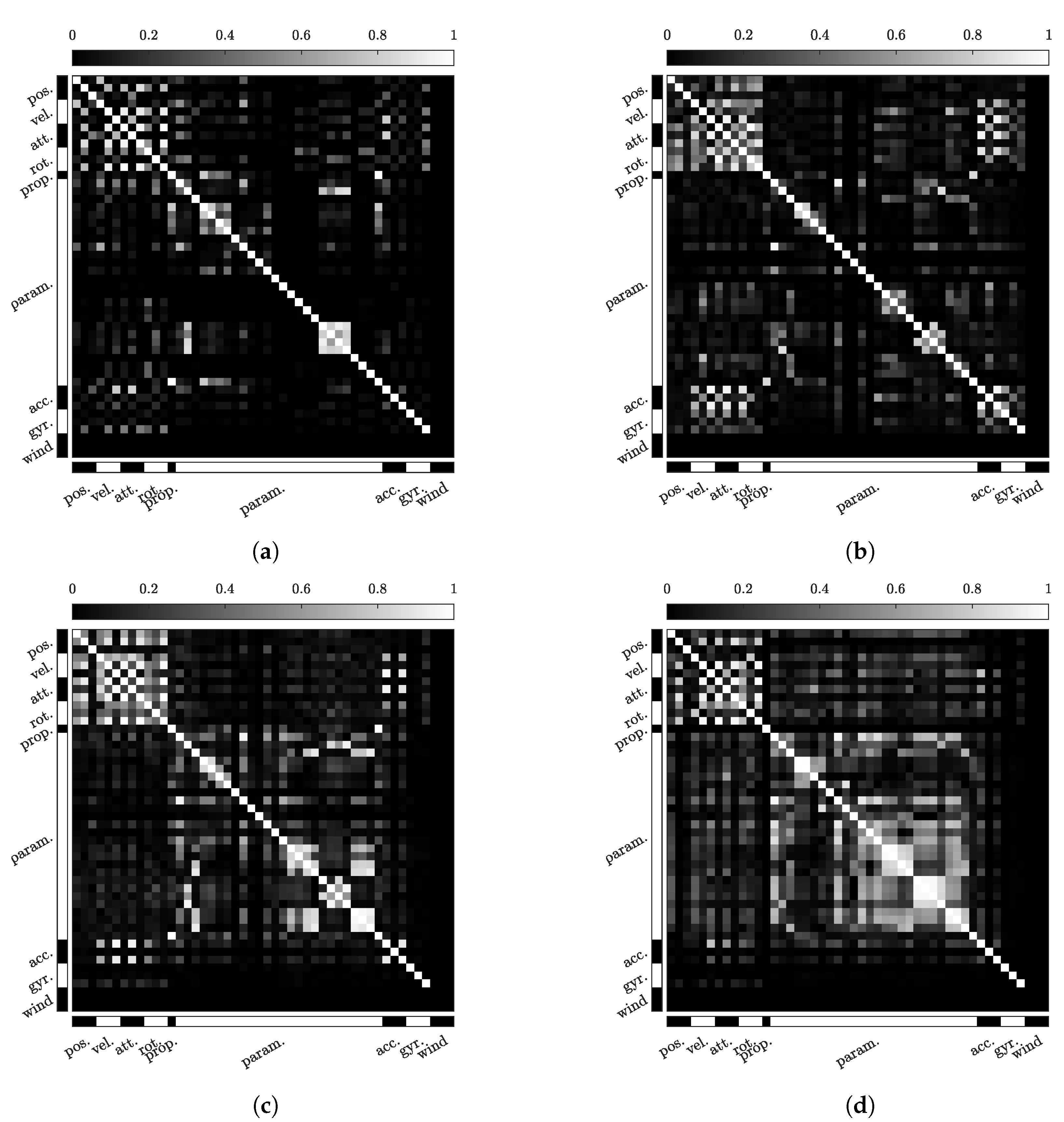
For a subset of trajectories, the correlation between all estimated states is shown in a grey scale of correlation matrix on Figure 4 at the end of the simulated trajectory.

In these figures, the diagonal elements represent the normalized variances of the estimated parameters, i.e., these have always value 1 and white color. The correlation coefficients (i.e., off-diagonal elements) are depicted by the varying grey scale from 0 to 1. As presented in Section 1 the state-vector $\mathit{X}$ is categorized in different groups, namely: navigation error states ${\mathit{X}}_n$, the VDM parameters ${\mathit{X}}_p$, the sensor errors ${\mathit{X}}_e$ and the wind states ${\mathit{X}}_w$. The first thirteen elements consist of navigation (position, velocity, attitude and angular rate) along with the estimated propeller speed n. The next 26 states correspond to the VDM parameters ${\mathit{X}}_p$. The next six states ${\mathit{X}}_e$ are the accelerometer and gyroscope biases estimated for each axis (The estimation of time-correlated errors only is the dominant part, even though other types of noise are added to the observations). The last three states are the wind components ${\mathit{X}}_w$, equal to zero as no wind condition is assumed. The distinguishable main square of 26 × 26 elements in the middle of the correlation matrix corresponds to the VDM parameter cross-correlation elements.

The correlation matrices show that trajectory directional dynamics increase the correlation among VDM parameters themselves and with the navigation states, which is initially set to zero. This is important, as VDM parameters become observable through such correlation when corrections to navigation states are made during GNSS update. At the same time, however, certain dynamics decrease the correlation of VDM parameters w.r.t. auxiliary states (i.e., other states than VDM coefficients). In other words, the group of VDM parameters stays correlated among them-self (the correlation among them is related to model definition. In this particular case the chosen polynomials are non-orthogonal, therefore their terms remain correlated implicitly), but become less dependent to auxiliary quantities (e.g., sensor errors) in the state-vector. This is important pre-requisite for their employment outside the calibration scheme.

Table 5. Highly correlated VDM parameter pairs for particular trajectories.

Level Flight				Asc. Straight Flight				‘8 loops’ with alt. Changes				Combination
$C_{M_{y}1}$	-	$C_{M_y\alpha }$	93.6%	$C_{M_{y}1}$	-	$C_{M_{y}e}$	90.4%	$C_{M_{y}e}$	-	$C_{M_y\alpha }$	90.2%	$C_{F_z\alpha }$	-	$C_{F_x\alpha 2}$	90.9%
				$\overline{c}$	-	$C_{M_y{\tilde{\omega }}_y}$	96.7%	D	-	$C_{F_{T}1}$	90.6%	$C_{M_x{\tilde{\omega }}_x}$	-	$C_{M_x{\tilde{\omega }}_z}$	90.9%
				$C_{M_{y}1}$	-	$C_{M_y\alpha }$	97.8%	$C_{M_{y}1}$	-	$C_{M_y\alpha }$	92.2%	$C_{M_z{\delta }_r}$	-	$C_{M_z\beta }$	95.2%
								$C_{M_z{\delta }_r}$	-	$C_{M_z\beta }$	95.4%	S	-	$C_{F_z\alpha }$	97.1%
								$\overline{c}$	-	$C_{M_y{\tilde{\omega }}_y}$	96.1%	$C_{M_{y}1}$	-	$C_{M_y\alpha }$	97.5%
								S	-	$C_{F_z\alpha }$	96.4%	$C_{M_{y}e}$	-	$C_{M_y\alpha }$	97.5%
								$C_{M_{y}e}$	-	$C_{M_y{\tilde{\omega }}_y}$	96.7%	$C_{M_{y}1}$	-	$C_{M_{y}e}$	97.9%
												$C_{M_x\alpha }$	-	$C_{M_x\beta }$	98.2%
												D	-	$C_{F_{T}1}$	99.4%

presents the VDM parameter pairs highly correlated (>90%) for a subset of trajectories.

For a particular trajectory, some VDM parameter pairs highly correlate, but not necessarily for another trajectory with different dynamic, i.e., the pair $\overline{c}-C_{M_y{\tilde{\omega }}_y}$, which converges with a correlation higher than 90% for a ascending straight line and “infinity loop” with altitude changes trajectory but its correlation decreases for a more complex one. Or, the pair $C_{M_{y}1}-C_{M_{y}e}$, which is well correlated for both the climbing line and the combination of trajectories, is not for the level and “infinity loop” ones. With these pairs, the highly correlated VDM parameters are good candidates to be re-unified within the Kalman filter into a common state. Such “parameter lumping” may prevent potential singularities and save processing power by reducing the states vector size and related matrices. Also, it may better to eliminate the geometrical parameters $\overline{c},S$ from unknowns and obtain their values from CAD models or other measurements.

3.3. Initial VDM Parameter Uncertainty

The state estimator, here an EKF, requires that the process model (described via VDM) fits adequately the physical behavior of the aircraft, otherwise it becomes unstable and can diverge [7]. Hence, the initial approximation of the VDM parameters (${\mathit{X}}_p$) need to be at some separation to the true, while in real scenarios, the true is unknown. The previous results have been conducted with randomly distributed initial uncertainty among the VDM parameters of 20 percent ($1\sigma$). Now, we alter such percentage with different values that range from 10 to 100. Subsequently, we count the number of Monte-Carlo simulations converging for all performed trajectories. The stability criteria is based on the navigation completion along the defined trajectory (reaching the last waypoint). This provides a sketchy idea on the required quality of initial coefficients (values and covariance).

Although 100 Monte-Carlos runs is a rather small number to generalize the findings, a trend can be observed from

Table 6. Number of successful navigation runs per initial error in VDM parameters per trajectories (Monte-Carlo 100 runs).

	Initial VDM Parameter Error $1\mathit{\sigma }$
Trajectory	10%	20%	30%	40%	50%	75%	100%
Descend. Straight L.	100	92	74	59	55	36	28
Straight line	100	98	71	56	53	36	26
Climbing Straight L.	100	98	87	70	60	40	31
Controlled Orbit	100	100	100	95	83	61	40
Orbit w. AutoPilot	100	99	95	79	57	31	19
8 Loop w. Alt. fix	100	100	99	86	73	43	31
8 Loop w. Alt. var.	100	100	98	79	66	41	21
Combinations	100	91	74	56	43	22	13

. Already from 20 percent of initial error ($1\sigma$), the filter stability can not be always guaranteed. The "controlled orbit" maneuver seems to be the more robust to initial error and is presented in light green. An explanation is that during this maneuver, the control inputs (actuators) are fixed and thus avoid instability due to a ‘contradiction’ between flight control inputs and the current (potentially ‘incorrect’) states.

A conclusion from Section 3.1 was, the higher the maneuver dynamic, the better the coefficients estimation. However, if the initial VDM parameter values are too far from the true ones, "higher-dynamic" maneuvers have higher non-linear impact on the divergence. This is particularly true for the combination of maneuvers, which possesses the lowest number of successful runs for almost all different scenarios. The smallest number of successful runs for the different trajectories for each initial error are presented in red in Table 6.

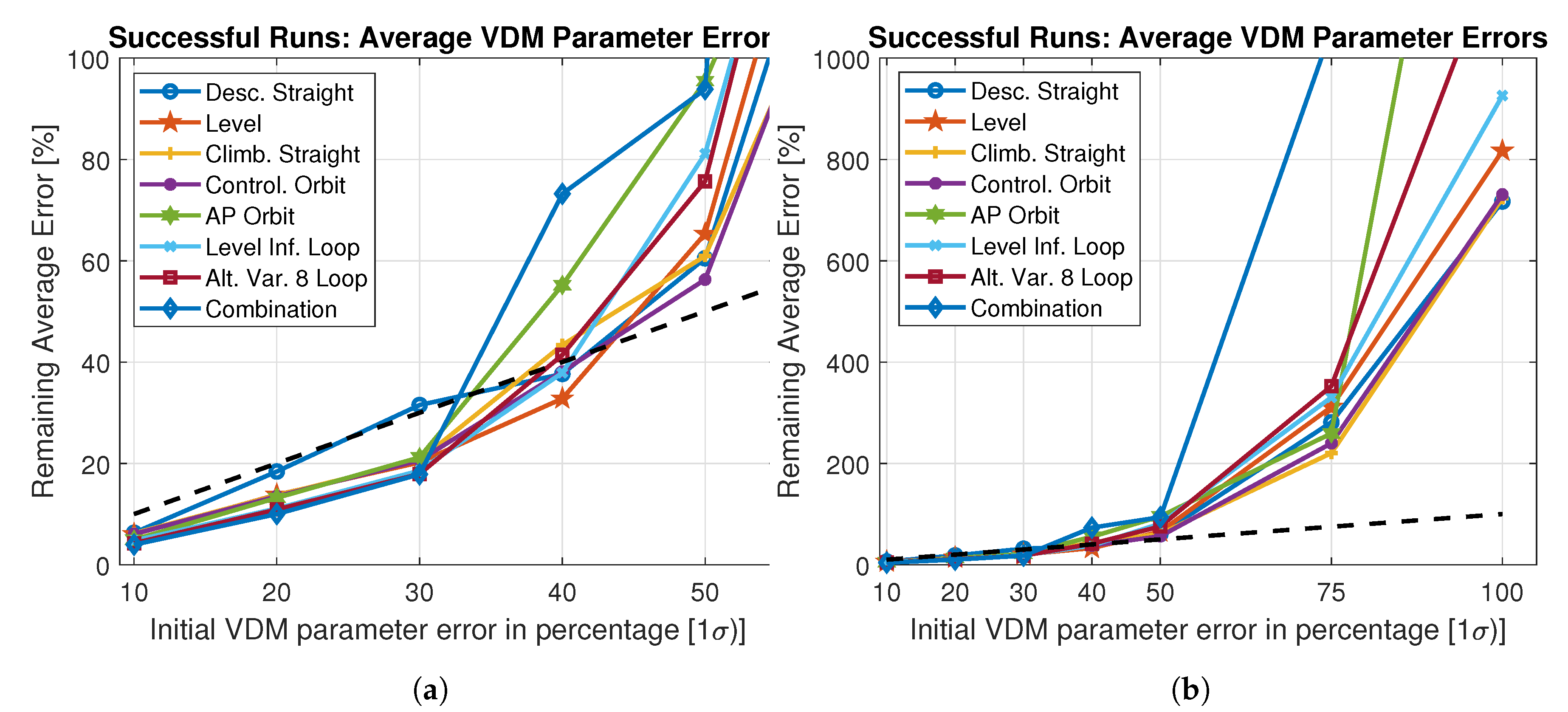
The remaining average VDM parameter error at the end of accumulated successful runs for different trajectories are depicted in Figure 5 and the filter divergence based on successful runs can be observed as a function of initial errors.

The black dashed-lines represent the initial VDM parameter error ($1\sigma$) applied randomly to the true values. Until 20 percent of initial error, as seen in Figure 5a, all trajectories converge to an average error bellow the initial value. Above about 35 percent, the remaining inaccuracy starts to be larger than their initial quantity. From 50 percent, the successful runs possess an average error above the initial values for all trajectories, suggesting the instability is reached (see Figure 5b). As a qualitative summary, in order to guarantee the filter stability and adequate navigation results, the initial uncertainties and errors in the VDM parameters should remain bellow 30 percent. Obviously, the better prior knowledge of the VDM parameters, the better for the filter stability and navigation performance. However, for real case scenarios, where the aerodynamic coefficients of an aircraft are not known or roughly approximated, this becomes a complex estimation challenge.

3.4. Sequence of Maneuvers

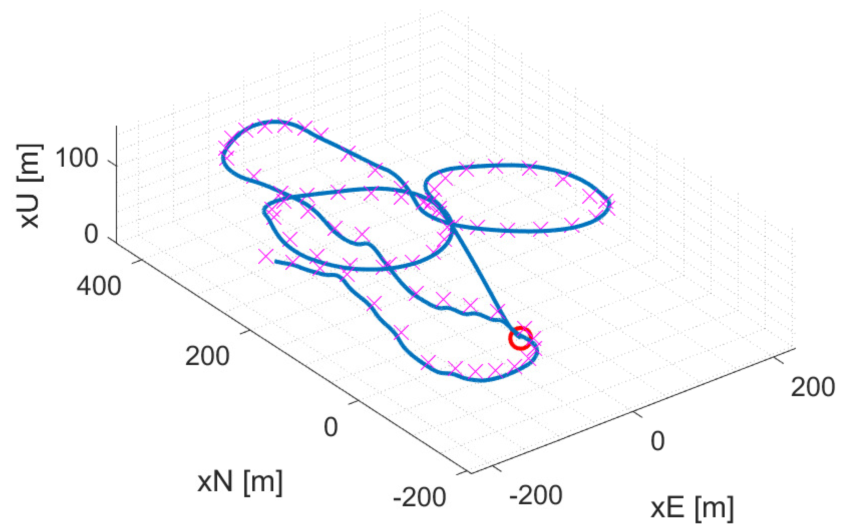
The previous analysis pointed out how different maneuvers contribute to the improved estimation of sub-groups of the VDM parameters. Therefore, the idea is to combine the segments of different shape into a "global" calibration maneuver. The proposed trajectory possesses a combination of the aforementioned trajectories with accelerations and de-accelerations, as well as upward and downward sections. The trajectory is depicted in Figure 6. The beginning of the trajectory, denoted with a red circle, starts with a climbing straight line, and the total flight time lasts around 3 min.

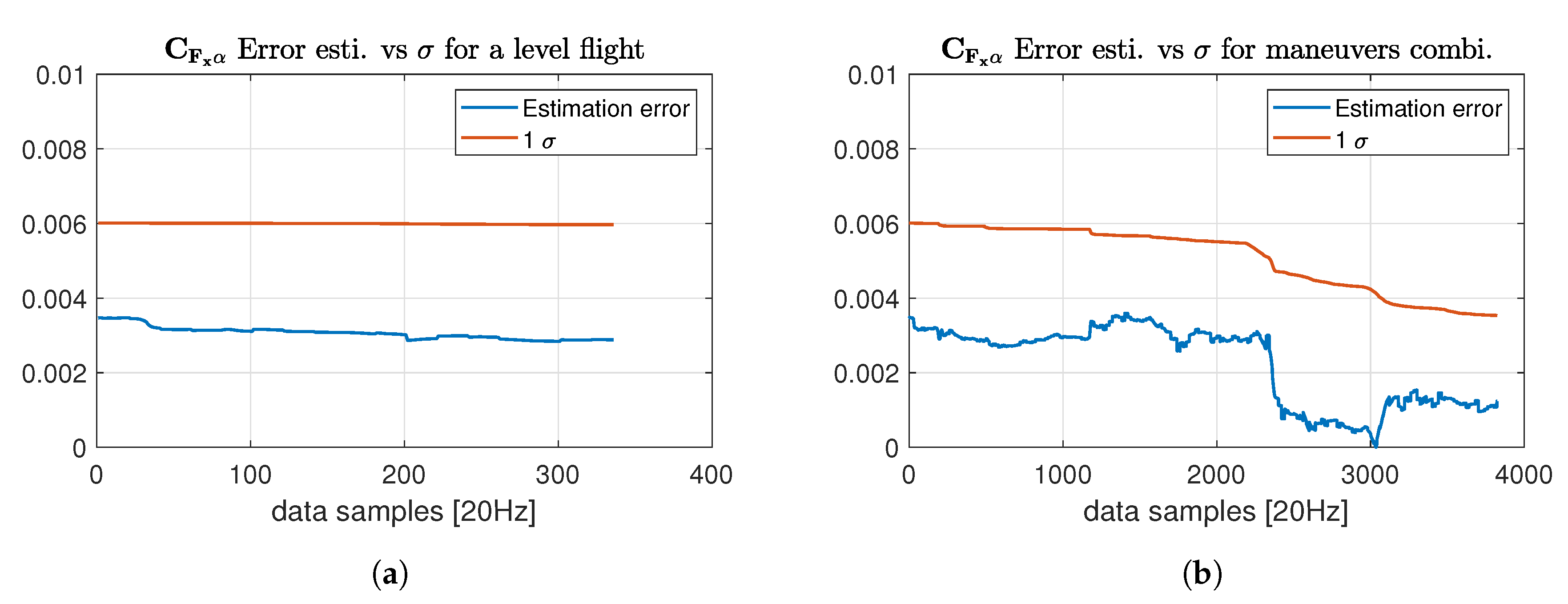
The effects of such a compound maneuver on the estimation of the VDM parameter $C_{F_x\alpha }$ is shown in Figure 7b with respect to a simple level flight, as seen in Figure 7a.

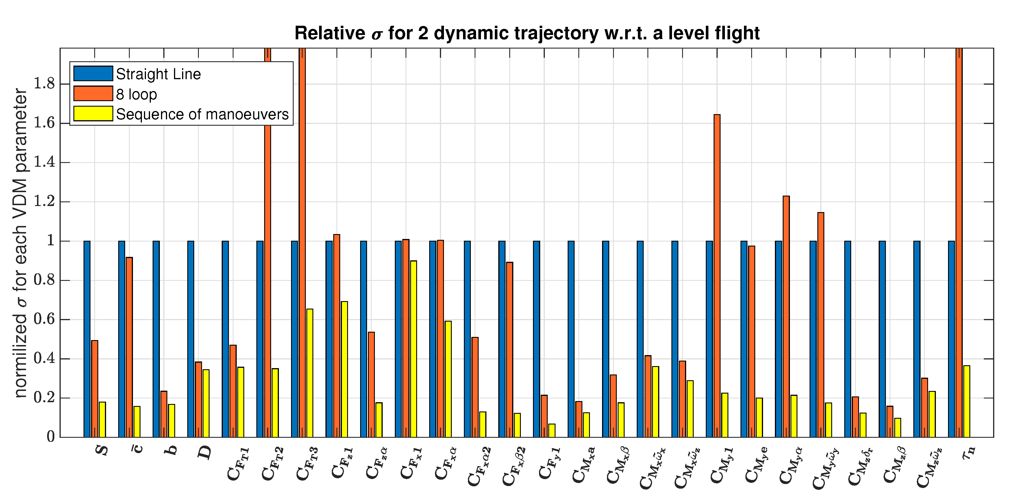
The uncertainty of this parameter represented by the estimated standard deviation (upper curve on both plots) is unchanged in the straight line, while reduced to 40% after maneuver sequencing. The latter case also removes approximately 50% of the parameter error (lower line), while the improvement of the former remains marginal. These investigations are generalized for every VDM parameter in Figure 8.

On this plot, the error for each VDM parameter is compared with the calibration result after a level flight in a constant direction for two types of sequences: an "infinity loop" at constant altitude and the previously described global calibration maneuver. The latter decreases the uncertainties in all VDM coefficients.

Although the (self-)imposed limitations on calibration duration (less than 5 min., Section 2.1) can be extended, it is observed that the absolute flight duration influences the obtained accuracy of the VDM parameters only marginally.

3.5. Brief Discussion on the Observability of VDM Parameters

A dynamic system is observable if its states can be uniquely established from the available sequence of observations. In the VDM-based navigation implementation, the state-vector is relatively large (>50) and its observability can be a concern.

We base the following discussion on the analysis of the obtained covariance matrices, residual state errors, and uncertainties.

The system is not completely observable at any time t. This is an unambiguous interpretation of the covariance matrix at the end of the level trajectory (Figure 4a). The lack of correlation among groups of coefficient reveals the lack of observability in the system for the considered case. Nevertheless, from Figure 8, we witness a relative reduction of the VDM parameter errors as the dynamic of the trajectory increases. This, in turn, suggests that the VDM parameters become observable (or their sub-groups) over a certain time interval with sufficient dynamic. This is equally applicable to the uncertainty reduction (standard deviation, $1\sigma$), as observed in Figure 7 for the coefficient $C_{F_x\alpha }$. Here, the time influence is perceptible and the same tendency is pertinent to all coefficients.

The correlation/decorrelation behavior of groups of coefficients depend on the trajectory shape as presented in Table 4. This fact is further supported by the covariance matrices (Figure 4) that shows different maneuvers with velocity changes need to be performed to observe all VDM parameters ${\mathit{X}}_{\mathit{p}}$.

The referred figures represent an average among the Monte-Carlo runs, but the stochastic aspects that are discussed above are also identical for each run.

4. Conclusions

We investigated the influence of maneuvers on the ability of self-calibrating model parameters in VDM-based navigation. We described the scenario of Monte-Carlo simulation while considering seven of typical flying scheme. The trajectory elements and necessary actuator states were generated while using simple guidance and control. From these, ideal sensor (INS/GNSS) outputs were obtained. Actuator and sensor readings were later corrupted by noise with different levels of correlation. The resulting data were processed by the VDM-based integration scheme, employing an Extended Kalman Filter as the principal estimator.

The analysis revealed that complex maneuvers alleviate the formation of correlation within groups of VDM parameters while accentuating their relations with navigation error states. Both facts improve the convergence to their true values. Indeed, a trajectory that combines different maneuvers emphasizes the dynamic changes during a calibration procedure that helps to fine-estimate the aerodynamic coefficients of a small UAV. The remaining highly correlated coefficients could be lumped into a common parameters. This would reduce the size of the state vector, which will, in turn, speed up filter execution—a fact to consider in real-time implementation. The removal of geometrical parameters ($S,b,\overline{c}$) is also possible when their values are obtained from direct measurements with sufficient accuracy.