Tightly-Coupled Joint User Self-Calibration of Accelerometers, Gyroscopes, and Magnetometers

Abstract

Inertial measurement units (IMUs) are fundamental for attitude control of drones. With the advancements in micro-electro-mechanical systems (MEMS) fabrication processes, size, power consumption, and price of these sensors have reduced significantly and attracted many new applications. However, this came at the expense of sensors requiring frequent recalibration, as they are highly contaminated with systematic errors. This paper presents a novel method to jointly calibrate the accelerometer, gyroscope, and magnetometer triad in a MEMS IMU without additional equipment. Opportunistic zero change in velocity and position updates, and inclination updates were used in conjunction with relative orientation updates from magnetometers in a robust batch least-squares adjustment. Solutions from the proposed self-calibration were compared to existing calibration methods. Empirical results suggest that the new method is robust against magnetic distortions and can achieve performance similar to a specialized calibration that uses a more accurate (and expensive) IMU as reference. The jointly estimated accelerometer and gyroscope calibration parameters can deliver a more accurate dead-reckoning solution than the popular multi-position calibration method (i.e., 54% improvement in orientation accuracy) by recovering the gyroscope scale error and other systematic errors. In addition, it can improve parameter observability as well as reduce calibration time by incorporating dynamic data with static orientations. The proposed calibration was also applied on-site pre-mission by simply waving the sensor by hand and was able to improve the orientation tracking accuracy by 73%.

1. Introduction

The market and applications for drones have skyrocketed. There are many manufacturers such as DJI, 3D Robotics, Yuneec, and Parrot SA each selling their own unique designs. Depending on the application, the drone may be equipped with extra sensors, such as laser scanners and cameras. Regardless of the manufacturer or application, modern day drones are all dependent on the inertial measurement unit (IMU) for assisting its attitude control. Conventional IMUs are composed of a triad of accelerometers and a triad of gyroscopes. Together they can autonomously determine accurate changes in position, velocity, and orientation of quadcopters and fixed wing unmanned aerial vehicles (UAVs) at high frequencies through strap-down integration. Although they can provide valuable navigation information, their long-term usefulness as a solo navigation device is jeopardized by the accumulation of errors over time. Even over a relatively short time interval, the sensor’s systematic errors are magnified by the integration process and will provide erroneous navigation parameters that can be deemed unusable. Therefore, it is extremely important that these systematic effects be minimized. In addition, popular onboard navaids deployed to aid IMUs (e.g., magnetometers) are only advantageous if they are properly calibrated for the platform they are mounted on. The necessity for manufacturers to perform precise and reliable laboratory calibration has become a significant portion of the production cost. Furthermore, unavoidable “wear and tear” from the usage of the sensor may lead to demands for recalibration. For lower cost systems, stress induced on the printed circuit board (e.g., soldering) can introduce parasitic effects on the accelerometer and gyroscope. Brodie et al., 2008 [1] recalibrated the accelerometer and gyroscope of a micro-electro-mechanical systems (MEMS) IMU and reported absolute static orientation errors of 5.2 degrees before user-calibration and 1 degree after; in addition, they claimed that their user-calibration parameters are valid for at least 22 days before another user-calibration is necessary. This paper presents a new robust low-cost quality assurance technique that users can perform without specialized tools or taking apart the drone.

2. Related Work

Traditionally, expensive external systems with accuracy better than the IMU under consideration are used to generate a series of reference signals. The IMU signals are forced to conform to this reference through solving for the systematic parameters [2], which may include:

• Accelerometer—biases, scale factors, and non-orthogonalities.
• Gyroscope—biases, scale factors, non-orthogonalities, axes misalignments, and g-sensitivities.
• Magnetometer—biases, scale factors, non-orthogonalities, axes misalignments, soft-iron effects, and hard-iron effects.

Typical calibration methods belonging to this category use actuated mechanical systems to position the IMU in known orientations and rotate at known and/or constant rotation rates [3,4,5,6]. Kim and Golnaraghi, 2004 [7] used the LED marker-based optical tracking system Optotrak to calculate the ground truth acceleration and angular rate of the IMU and calibrated the biases, scale errors, and non-orthogonality for the accelerometer and gyroscope in a disjoint nonlinear least-squares routine. Existing infrastructure such as GNSS can also be used but will be restricted to outdoor environments [8,9]. Well-known methods in this category of inertial calibration include the local level frame method, six-position static test, and rate test [10]. Special boxes/mounts/platforms where the IMU can be mounted and rotated or positioned accurately in a deterministic fashion can also be used [11,12]. For magnetometer calibration, a 3D Helmholtz coil can be used to generate a known magnetic field in various directions [13]. These methods all require infrastructure and/or apparatus that may not be readily available to the end-user.

Another, perhaps more suitable, stream of self-contained user calibration methods focused on exploiting reference signals found in nature and has no demand for specialized equipment except for the sensors on-board. For example, Panahandeh et al., 2010 [14] implemented a gravity constraint in the local-level frame to calibrate a triad of accelerometers. The calibration of other sensors necessary to obtain the full navigation solution was not studied, and the presented approach requires solving the nuisance inclination angles for every orientation besides the 9 accelerometer calibration parameters. Yang et al., 2012 [15] performed a similar 2-step optimization procedure for the calibration parameters and then the inclination but also solved for the non-linear scale errors. Wu et al., 2002 [16] and Lötters et al., 1998 [17] avoided the need to determine the orientation angles during calibration by constraining the norm of acceleration under static or quasi-static periods to equal gravity.

The magnetometer can be calibrated by using the same concept of constraining the norm to a constant value (e.g., the magnitude of the Earth’s magnetic field obtained from a geomagnetic model) [18]. Instead of negligible or zero motion, a constant and uniform ambient magnetic field is required for the calibration [19]. This approach is comparable to performing a geometric sphere-fit to 3D points [20]. When used as an orientation update, the strength of the field has no impact, so the magnitude can arbitrarily be constrained to unity [21]. Any motion that can generate sufficient samples to cover the entire surface of the sphere can be used to determine the hard and soft iron effects reliably, although Ali, 2013 [22] tested several movement patterns (i.e., random, figure-eight, and orthogonal excitations) and concluded that coordinated rotation works best.

When the sensor is stationary, the gyroscopes should only sense the rotation rate of the Earth and the magnitude of the observed angular rate can be compared to this reference using the same norm constraint previously described [23].

These methods can calibrate a particular module (e.g., triad of magnetometers or accelerometer) of a 9-DoF IMU or they can be combined to calibrate multiple modules (albeit independently). Camps et al., 2009 [24] used the aforementioned norm constraint approach to calibrate a triad of accelerometers and magnetometers. In the popular multi-position (or perhaps, “multi-orientation”) calibration approach the accelerometer and gyroscope were calibrated at the same time using the magnitude constraint [23]. These methods can be combined to calibrate a 9-DoF system, although in the case of magnetometers, the static requirement is unnecessary. This combined approach independently calibrates the accelerometer, gyroscope, and magnetometer even though data from the same trial can be used. It was reported that ~19% performance improvement can be expected for tactical-grade IMUs [25], but the gyroscope scale error and axes non-orthogonality for both the accelerometer and gyroscope are difficult to estimate using this method [26]. Rather than requiring strict-static periods, automatically detectable quasi-static periods can be used for convenience (with minor compromises in accuracy) for pedestrian tracking applications [27,28]. Most improvements made to this method involve adding a turn-table to generate a stronger reference signal for the gyroscope [29,30,31]. Undeniably this is advantageous, but reduces the ease-of-use factor by returning to the reliance on additional equipment. It took Zhang et al., 2010 [30] almost 2.5 h of data capture to perform their modified multi-position calibration.

Another stream of inertial sensor calibration exploits the correlation between the sensor’s accelerometer, gyroscope, and/or magnetometer to perform the calibration. In such cases the calibration of the IMU components are no longer decoupled and often the inter-triad misalignment needs to be known or estimated in addition to tracking the orientation states. Examples of this type of calibration include Kok et al., 2012 [32] and Kok and Schön, 2014 [33]. In Kok et al., 2012 [32], the authors calibrated the magnetometers using sphere-fitting and the dip angle constraint along with the inclination (estimated by running a Kalman filter on the inertial data) to derive the axes misalignments. Since the inclination was estimated independent from the magnetometer calibration, the magnetometer readings were not used to update the inclination and calibrate the inertial sensor. In Kok and Schön, 2014 [33], they used a grey-box system identification approach to estimate the 12 magnetometer calibration parameters as well as the gyroscope bias and variance-covariance matrices of the accelerometer, gyroscope, and magnetometer. In both cases systematic errors of the accelerometers were ignored and small accelerations were expected, otherwise the estimated vertical direction could be erroneous.

Cheuk et al., 2012 [34] hierarchically calibrated a 9-DoF IMU by first constraining the accelerometer and magnetometers to fit on two separate spheres and then comparing changes in orientation from integrating the gyroscope signal with the orientation determined by the accelerometer and magnetometer combined. They only used the magnetometer and accelerometer when the sensor was static (dynamic portions of the data were simply ignored).

Renaudin and Combettes, 2014 [35], used a pre-calibrated magnetometer to help estimate the accelerometer and gyroscope biases in a Kalman filter. Their magnetic angular rate model and acceleration gradient model are comparable to the magnetometer and levelling updates used in this paper, which are suitable attitude updates (AUPT) for indoor urban environments. However, they focused on the tracking solution and did not account for the scale errors and non-orthogonalities of the triads. More recently, Li et al., 2015 [36] improved upon this approach by using a pre-calibrated magnetometer to also estimate the accelerometer and gyroscope scale errors. Measurement updates include approximate position updates, low-pass acceleration updates, quasi-static orientation updates, and relative change in magnetic field update when periods of constant magnetic field is identified by a detector. However, besides assuming that a calibrated magnetometer is available, not all systematic errors were estimated by the filtering approach.

So far, none of the presented calibration routines can simultaneously calibrate for the accelerometer, gyroscope, and magnetometer sensors along with their inter-triad misalignments optimally without specialized tools; both Zhang et al., 2014 [37] and Ammann et al., 2015 [38] stressed the importance of determining the inter-triad misalignments but neglected some dependencies between the sensors by not calibrating them simultaneously. The abovementioned shortcomings can be mitigated using the proposed methodology.

3. Proposed Method

The proposed self-calibration method was performed offline using a robust batch optimization technique. Compared to a filtering approach, this allows information from the past, present, and future to be incorporated optimally for identifying the systematic errors. By following the implicit least-squares adjustment framework, all navigation states (i.e., orientation, velocity, and position) can be marginalized away from the beginning of the adjustment, eliminating the need to determine good initial approximations for the non-linear optimizer and making the size of the Hessian and Jacobian time-invariant. To the authors’ best knowledge, this is the first total-system user self-calibration method designed for MEMS IMU with a magnetometer that can simultaneously model all first order systematic errors. Forty-two parameters are considered in this paper: accelerometer—3 biases, 3 scale errors, 3 non-orthogonality angles; gyroscope—3 biases, 3 scale errors, 3 non-orthogonality angles, 9 g-sensitivity coefficients, 3 angles for axes misalignment relative to the accelerometer; magnetometer—9 elements for the soft-iron effects and 3 elements for the hard-iron effects. In addition, both static and dynamic data from all three sensor triads are used; there is no restriction on how the sensor needs to be moved apart from having occasional periods of stillness (as in the typical multi-position calibration). The novelty of the presented 9-degrees-of-freedom (DoF) IMU calibration method is the combination of the following:

• Tightly-coupled joint calibration (rather than sequential independent hierarchical calibration) of accelerometers, gyroscopes, and magnetometers.
• Number of optimization variables is time invariant and only contains the calibration parameters; this eliminates efforts in rotation parameterization, datum definition, and deriving initial approximation for the navigation states.
• Assumes only piecewise local homogenous magnetic field rather than a single global homogenous field, which is more suitable for indoor applications.
• Automatic outlier detection for abrupt magnetic disturbances during optimization.
• Opportunistic zero change in velocity, inclination, and loop-closure position updates when deemed suitable for calibrating the MEMS IMU indoors.
• Calibration is self-contained and easy to perform by the end-user. By combining both static and dynamic signals a total of 42 systematic error parameters can be recovered without using expensive equipment.

3.1. Sensor Models

The following sensor models describe the relationship between the observed signals (e.g., sensed angular velocity and acceleration) and the true signal by accounting for the systematic and random errors. In the following equations, uppercase letters represent 3 by 3 matrices and lowercase letters represent 3 by 1 vectors. Furthermore, S is a diagonal matrix and N is a lower-triangular non-orthogonality matrix, where both are composed of three independent unknown parameters [30]. Although the effect of scale error and axes non-orthogonalities can be merged into a single matrix, they are treated separately for the accelerometers and gyroscopes to be consistent with the notation in some literature (e.g., [23,29]).

3.1.1. Accelerometers

$${}^{s}y_a=S_a{N}_a{}^{s}a+b_a+{\epsilon }_a$$

(1)

where,

• ^sy_a is the measured acceleration in sensor frame.
• S_a is the linear accelerometer scale factor.
• N_a is the accelerometer axes non-orthogonality.
• ^sa is the true acceleration in sensor frame.
• b_a is the accelerometer bias.
• ε_a is the accelerometer noise.

3.1.2. Gyroscopes

$$y_{\omega }=S_{\omega }{N}_{\omega }{R}_{\omega }{}^s\omega +b_{\omega }+G_{\omega }{}^{s}a+{\epsilon }_{\omega }$$

(2)

where,

• y_ω is the measured angular rate in gyroscope frame.
• S_ω is the gyroscope scale factor.
• N_ω is the gyroscope axes non-orthogonality.
• R_ω is the inter-triad misalignments between the accelerometers and gyroscopes.
• ^sω is the true angular rate in sensor frame.
• b_ω is the gyroscope bias.
• G_ω is the g-sensitivity.
• ε_ω is the gyroscope noise.

3.1.3. Magnetometers

$$y_m=D_m{}^{s}m+o_m+{\epsilon }_m*$$

(3)

where,

• y_m is the measured magnetic field in magnetometer frame.
• D_m is the soft-iron effects.
• ^sm is the true magnetic field in sensor frame.
• o_m is the hard-iron effects.
• ε_m is the magnetometer noise.

* Note that D_m and o_m also convey the effect of magnetometer biases, scale factors, axes non-orthogonality, and inter-triad misalignments.

3.2. Constraints and/or Measurement Updates

Conventional IMU mechanization found in a Kalman filter requires the 3D pose (i.e., 7 parameters when using quaternions) and velocity (i.e., 3 parameters) to be estimated at every epoch (Equation (4)). Often IMU biases (i.e., 3 gyroscope biases and 3 accelerometer biases) are treated as time-varying unknowns (e.g., random walk process) and are included in the filter, resulting in 16 unknowns at every time step. These equations can pose a challenge when implementing in a batch least-squares adjustment; for example, the number of unknown parameters for a 100 Hz IMU can reach 96k in a minute (assuming orientations are parametrized using quaternions, represented by q in the equations). If all 42 calibration parameters are being considered this increases to 312k unknowns per minute. Furthermore, navigation states of an uncalibrated IMU will have to be initialized using some approximate methods before the nonlinear least-squares estimations.

$$\begin{gathered} {}^{L}p_{t+T}={}^{L}p_t+{}^{L}v_{t}T+\frac{1}{2}\left({}^{L}q_{t+T}·d{v}_{t,t+T}·{}^{L}q_{t+T}^c+{}^{L}g{T}^2\right) \\ {}^{L}v_{t+T}={}^{L}v_t+{}^{L}q_{t+T}·{}^{L}d{v}_{t,t+T}T·{}^{L}q_{t+T}^c+{}^{L}gT \\ {}^{L}q_{t+T}={}^{L}q_t\otimes \exp \left(\frac{1}{2}d{q}_{t,t+T}T\right) \end{gathered}$$

(4)

where,

• ^Lp, ^Lv, and ^Lq are the unknown navigation states (position, velocity, and orientation using quaternion parametrization, respectively) in local frame at time t and t + T.
• dq_t,t+T and dv_t,t+T are the change in orientation and velocity (defined in Equations (8) and (11), respectively).
• ^Lg is the local gravity vector.
• T is the time interval.

Please note: superscript c indicates the quaternion conjugate.

Instead, the constraints and measurement updates in this section are written in implicit form (i.e., f(X,Y) = 0, where X and Y are the unknowns and observations, respectively). This was chosen by design in order to use an implicit least-squares solver [39] to eliminate the necessity to explicitly solve for the navigation states, which grows with time. The constraints and updates described below may happen at different times (i.e., opportunistically), and only the magnetometer updates are being applied at regular intervals. 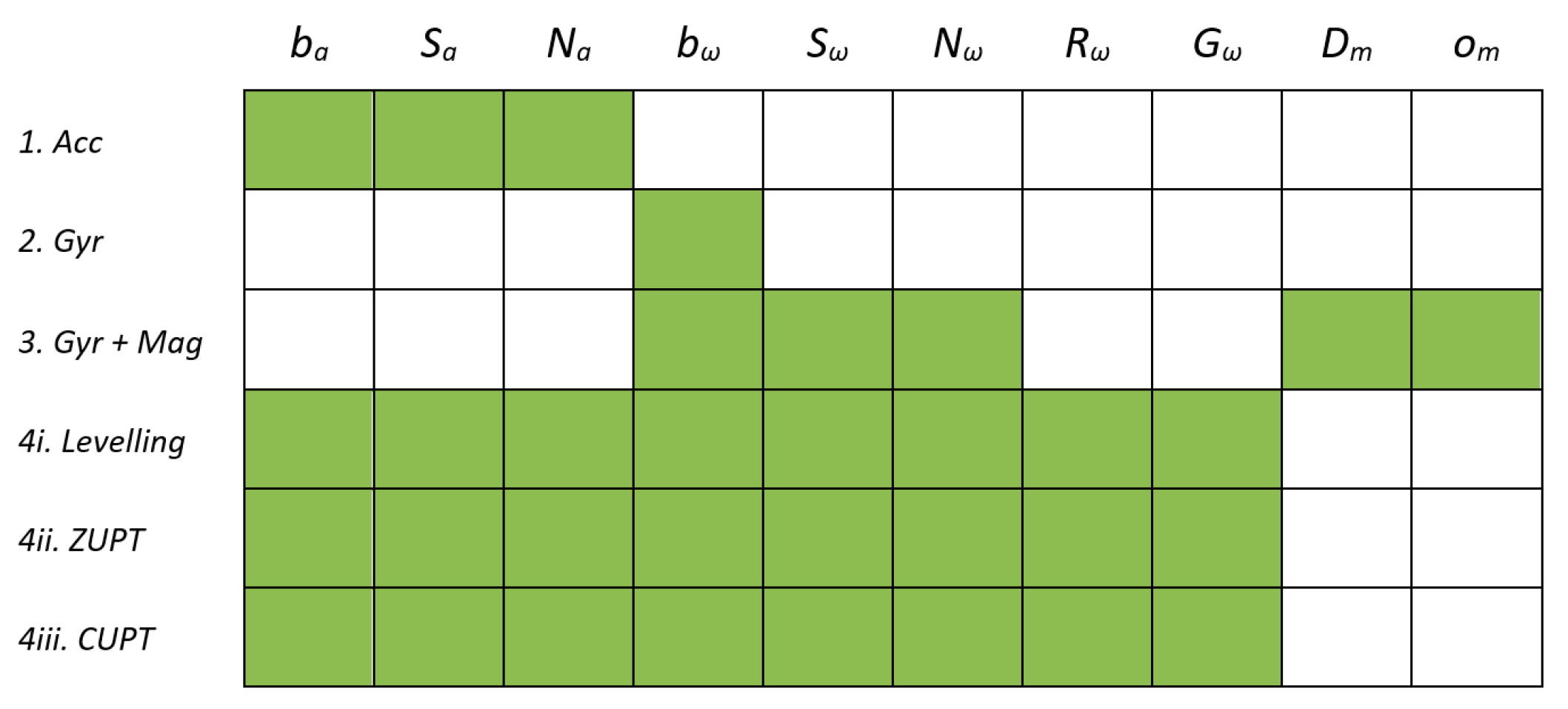The different constraints/updates are influenced by different systematic sensor errors and therefore provide different information to the self-calibration in terms of their recovery (Figure 1). Their combined effect makes all the systematic errors observable in the total-system user self-calibration and some redundancy between observability improves the reliability of the estimates. More details about each individual update or constraint are given in the following subsections.

3.2.1. Accelerometers

When static or quasi-static periods in the IMU data are detected (e.g., by considering a window of inertial data and checking the variance against some threshold [9]), the magnitude of the measured acceleration in sensor frame (s) should equal the local gravity (^Lg). This update can help define the scale for the accelerometer.

$${\Vert {}^{s}a\Vert }_2^2-{}^{L}g^2={}^{s}a_x^2+{}^{s}a_y^2+{}^{s}a_z^2-{}^{L}g^2=0$$

(5)

where, ^sa_x, ^sa_y, and ^sa_z are the individual components of the corrected acceleration in sensor frame.

3.2.2. Gyroscopes

When static or quasi-static periods in the IMU data are detected, the magnitude of the measured angular rate should equal the rotation rate of the Earth. However, for MEMS IMUs the noise typically masks such a weak signal. Instead the three components (x, y, and z channel) can be conditioned to zero (a.k.a. zero rotation update). Any non-zero mean value will indicate a bias.

$${}^s\omega _x={}^s\omega _y={}^s\omega _z=0$$

(6)

where, ^sω_x, ^sω_y, and ^sω_z are the individual components of the corrected angular rate in sensor frame.

3.2.3. Gyroscopes + Magnetometer

Regardless of the motion, the gyroscope signals and magnetometer signals can be compared to each other in both static and dynamic situations. Instead of requiring the sensor to be static, the local magnetic field should be constant and homogenous. If this assumption is satisfied, the magnetometer can act as a low-pass filter that smooths out the sensed angular rate, while the gyroscope captures the high-frequency dynamics missed by the magnetometers. Although such an assumption may be satisfied in outdoor applications, in indoor urban environments the homogenous magnetic field assumption is often violated. Instead, the assumption can be relaxed to assume only piece-wise constant magnetic fields at the expense of losing the absolute heading reference (i.e., magnetic north) and experiencing the possibility of heading drift. However, since the calibration parameters are defined in sensor frame, they are independent of the absolute reference.

Assuming a longer duration of homogeneous magnetic field reduces heading drift and induces more smoothing; however, it is more likely to be violated due to magnetic disturbances. On the contrary, by assuming a shorter duration, the update has a higher probability of being valid but the heading will drift more rapidly. It has also been perceived that a longer duration assumption is more robust to magnetic disturbances because, with a larger rotation interval, the outliers become more detectable. To combine the benefits of both approaches, the magnetometer updates can be performed at two frequencies simultaneously (e.g., 10 Hz and 100 Hz as in this paper). The magnetic field measurements at different times can be related through a 3D rotation (Equation (7)) determined by performing strap-down integration on the gyroscope signal (Equation (8)).

$$d{q}_{t,t+T}·{}^{s}m_{t+T}·d{q}_{t,t+T}^c-{}^{s}m_t=0$$

(7)

$$d{q}_{t,t+T}=\frac{1}{2}{\displaystyle \underset{\tau =t}{\overset{T}{\int }}d{q}_{t,\tau }·}{}^s\omega _{\tau }d\tau$$

(8)

where,

• dq_t,t+T is the relative change in orientation from time t to time t + T expressed using quaternions (with the superscript c representing the conjugate).
• ^sω_τ is the vector of corrected angular rates at time τ expressed in sensor frame.
• ^sm_t is the vector of corrected magnetic samples at time t expressed in sensor frame.

3.2.4. Accelerometer + Gyroscopes

Several updates based on the accelerometer and gyroscope can be enforced depending on the user’s motion for calibrating both sensors, namely levelling update, zero-velocity update (ZUPT), and coordinate update (CUPT).

i. Levelling Update

When the sensor is static the accelerometers can define the tilt angles relative to the local-level frame by measuring gravity. This can be used to update the inclination determined from integrating the gyroscope readings and give the orientations an absolute vertical reference.

$$d{q}_{t_1,t_i}·{}^{s}a_{t_i}·d{q}_{t_1,t_i}^c-{}^{s}a_{t_1}=0$$

(9)

ii. Zero-Velocity Update (ZUPT)

Between two static (or quasi-static) periods the total change in velocity is zero. Instead of directly applying the update to the velocity, which would involve solving for all the nuisance intermediate velocity and orientation parameters, this update can be applied directly to the accelerometer and gyroscope signals using Equation (10) and strap-down integration for change in velocity (Equation (11)).

$${}^{s}g_{t_1}·\left(t_i-t_1\right)+d{v}_{t_1,t_i}=0$$

(10)

$$d{v}_{t_1,t_i}={\displaystyle \underset{\tau =t_1}{\overset{t_i}{\int }}d{q}_{t_1,\tau }·{}^{s}a_{\tau }·d{q}_{t_1,\tau }^{c}d\tau }$$

(11)

where,

• $d{v}_{t_1,t_i}$ is the change in velocity from time t₁ (first epoch) to time t_i expressed in the sensor frame at t₁.
• ${}^{s}g_{t_1}$ is the gravity vector at time t₁ expressed in sensor frame.

iii. Coordinate Update (CUPT)

If the user is rotating the sensor while standing or sitting at the same location, and/or the sensor was returned approximately to the same position after a period of time, an approximate zero change in position update can be applied. In the former case, this update can be applied at regular intervals, and in the latter it can be applied sporadically even if the sensor is not static. Following the strap-down integration approach described above and assuming the sensor started at rest, the CUPT can be implemented without explicitly solving for the navigation states using Equations (12) and (13). The detection of loop-closure (e.g., based on magnetic signature or RSS fingerprint) was not studied in this research, similar position updates were detected manually based on the data acquisition procedure described in Section 4.

$$\frac{1}{2}·{}^{s}g_{t_1}·{\left(t_j-t_1\right)}^2+d{p}_{t_1,t_j}=0$$

(12)

$$d{p}_{t_1,t_j}={\displaystyle \underset{\tau =t_1}{\overset{t_j}{\int }}{\displaystyle \underset{\xi =0}{\overset{\tau }{\int }}d{q}_{t_1,\xi }·{}^{s}a_{\xi }·d{q}_{t_1,\xi }^{c}d\xi d\tau }}$$

(13)

where, $d{p}_{t_1,t_j}$ is the change in position from time t₁ to time t_j expressed in the sensor frame at t₁.

3.3. M-Estimator

The calibration parameters for the accelerometer, gyroscope, and magnetometers are treated as time-invariant and can be solved simultaneously offline using the standard iterative Gauss-Helmert least-squares adjustment [39] (as in the multi-position calibration approach [29]). The nuisance parameters (i.e., states) were marginalized away by design from the beginning (i.e., by writing the functional models in implicit form), which constrain the dimensions of the Hessian matrix. The unknowns vector contains the 42 calibration parameters only (i.e., X = [b_a, S_a, N_a, b_ω, S_ω, N_ω, G_ω, R_ω, D_m, o_m]^T) and the observations are the accelerometer, gyroscope, and magnetometer readings (i.e., Y = [y_a, y_ω, y_m]^T), along with the pseudo-measurements for the approximate CUPT. During the batch optimization the sum of weighted residuals squared is minimized (Equation (14)) subject to Equation (15). For more information about applying this implicit least-squares formulation to IMU data, please refer to Shin and El-Sheimy, 2002 [23] and Shin, 2001 [26]. Through marginalization the Hessian loses its sparse structure, however the size of the resulting dense Hessian matrix will never exceed 42 by 42 regardless of the amount of data captured. This is a favorable property and offers the potential for this method to be scaled to larger datasets.

$${\widehat{r}}^T{C}_l^{-1}\widehat{r}=\min$$

(14)

$$A\widehat{\delta }+B\widehat{r}+w=0$$

(15)

where,

• $\widehat{\delta }$ is the correction to the unknown parameters, X.
• $\widehat{r}$ is the correction to the observations, Y.
• w is the misclosure vector.
• A is the first design matrix.
• B is the second design matrix.
• C_l is the observations variance-covariance matrix.

The measurement noise of the sensors can be obtained from the manufacturer’s specification sheets or from studying the Allan Variance. The noise introduced for the approximate CUPT depends on the application and is the only parameter that requires tuning (it was set to σ = 10 cm in this paper). All other measurement updates were assumed to be exact. To improve the robustness of the estimator, the Huber and Tukey weight functions [40] were adopted to iteratively reweight the accelerometer and magnetometer observations, respectively. This approach is suitable for dampening the effects of abrupt magnetic disturbances and false-detection of static periods that can significantly affect the calibration, for example.

4. Experimentation

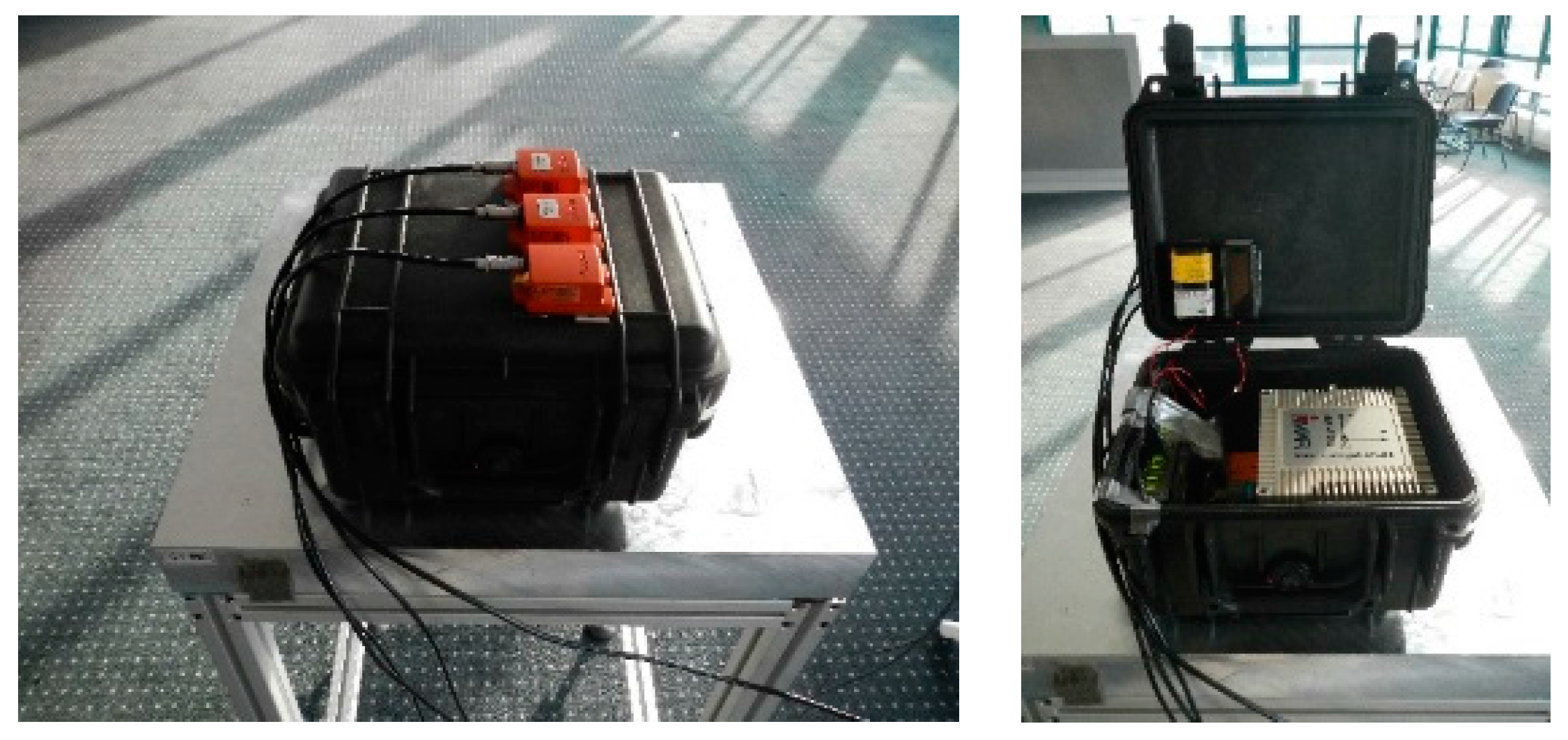
Two MEMS-based IMUs from Xsens Technologies, MTi-300 and MTi-G-700 (both with built-in accelerometers, gyroscopes, and magnetometers), were used for testing the algorithm. All data were logged at 100 Hz (note: the raw inertial data was captured at 2 kHz and then down-sampled to 100 Hz via strap-down integration [41]). For quality control, a fiber optic gyroscope (FOG)-based tactical grade IMU (i.e., IMU-FSAS from iMAR GmbH, St. Ingbert, Germany) capturing at 200 Hz was rigidly attached to the MEMS IMU to provide a reference solution (Figure 2). The two IMUs were software time synchronized for each experiment, while their rotational and translational offsets (i.e., boresight and lever-arm) were predetermined using the calibrated accelerometer and gyroscope signal. All reported error measures were computed by differencing the MEMS IMU solution with the tactical-grade IMU solution.

4.1. Case 1: In-Laboratory User Self-Calibration

In the first case, data was acquired by placing the MTi-G-700 in various static orientations (i.e., 15) similar to the conventional multi-position IMU calibration scheme. This calibration was performed in a controlled environment with the objective of estimating the static portion of the systematic errors (e.g., axes non-orthogonality). The repeatability and robustness of the calibration was tested by carrying out ten consecutive calibrations with the MTi-300. The first five trials were acquired while mitigating magnetic disturbances (i.e., rotating the sensor with minimal translations in an open space) and for the remaining five trials the sensor was rotated and translated in the presence of various magnetic disturbances (e.g., computers, tables, chairs, etc.). The latter heterogeneous magnetic field case can represent some unexpected magnetic field changes during laboratory calibration. In addition, it illustrates the potential of extending this method in an uncontrolled environment when significant excitations are provided.

4.2. Case 2: On-Site User Self-Calibration

The second experiment was designed to reduce the time and effort of the multi-position calibration (i.e., less stillness periods), which despite being easy to perform, may not always be a viable option on-site. The MTi-G-700 begins in a static or quasi-static position, followed by a sequence of hand-held rotations (~30 s) to ensure all axes are excited, and finishes in a static position near the starting position. This type of calibration is suitable for estimating the static systematic errors that may change from operation to operation such as turn-on biases and the soft and hard-iron effects immediately prior to data acquisition for example. A special case where no periods of stillness exist in the MTi-300 data is also presented to show the performance of the method as a gyroscope and magnetometer duo calibration method. This accelerometer-free calibration places no restriction on the motion (e.g., slow movements or quasi-stillness) and is suitable for applications with unpredictable extreme dynamics.

5. Results and Analyses

5.1. Case 1: In-Laboratory User Self-Calibration

Although the data acquisition procedure is almost identical to the popular multi-position self-calibration approach, the data processing of the proposed method is rather different. The conventional method ignores all dynamic data and the mutual information that can be shared between the sensors. The proposed method can achieve similar or better accuracy in less time by exploiting both static and dynamic portions of the trial in the optimization.

The multi-position calibration (without turn-tables) has difficulties estimating the gyroscope scale errors (and possibly the accelerometer and gyroscope axes non-orthogonality). Through the inclusion of accelerometer, gyroscope, and magnetometer signals under motion (Equations (6), (8), (9) and (11)), the accelerometer and gyroscope biases, scale errors, non-orthogonality, and inter-triad misalignments can be recovered simultaneously with the hard and soft-iron effects for the magnetometer. The estimated calibration parameters along with their standard deviations are reported in

Table 1. Estimated residual systematic errors for the Xsens MTi-G-700 using the proposed method in-lab.

Component	Accelerometer			Gyroscope						Magnetometer
	Ba (m/s2)	Sa (unitless)	Na (deg)	Bω (deg/s)	Sω (unitless)		Nω (deg)		Rω (deg)	om (a.u.)
X	−0.0639	0.0007	−0.0135	−0.0759	0.0003		0.0241		0.0060	−0.0216
Y	−0.0028	0.0006	0.0292	−0.0003	0.0000		−0.0053		−0.0114	0.0147
Z	0.0446	0.0002	0.0012	−0.2532	0.0002		−0.0451		0.0779	−0.0139
	σ			σ						σ
X	1.45 × 10−4	1.71 × 10−5	3.72 × 10−3	7.31 × 10−4	5.27 × 10−5		4.14 × 10−3		4.82 × 10−3	4.23 × 10−5
Y	2.41 × 10−4	1.99 × 10−5	4.69 × 10−3	7.45 × 10−4	5.98 × 10−5		4.15 × 10−3		4.43 × 10−3	4.00 × 10−5
Z	1.11 × 10−4	1.23 × 10−5	1.93 × 10−3	8.78 × 10−4	5.73 × 10−5		4.11 × 10−3		5.52 × 10−3	3.81 × 10−5
				Gω (rad∙s/m)						Dm (unitless)
Matrix				0.0000		0.0000		0.0000		−0.0358	−0.0093	−0.0173
				0.0000		0.0000		0.0000		−0.0003	−0.0194	−0.0507
				0.0000		0.0000		0.0000		−0.0142	−0.0134	0.0552
				σ						σ
Matrix				2.80 × 10−6		2.41 × 10−6		2.52 × 10−6		5.44 × 10−5	9.03 × 10−5	9.20 × 10−5
				2.95 × 10−6		3.51 × 10−6		2.82 × 10−6		1.02 × 10−4	6.07 × 10−5	1.04 × 10−4
				1.82 × 10−6		1.71 × 10−6		2.16 × 10−6		9.57 × 10−5	9.63 × 10−5	5.71 × 10−5

. The sensor under consideration appears to be well calibrated, with the most pronounced systematic errors being the accelerometer and gyroscope biases, and the magnetic distortions induced by the mounting platform.

All the recovered systematic errors are statistically significant based on the t-test at a 95% confidence interval, except for a few terms in the g-sensitivity matrix, the non-orthogonality between the accelerometer’s y- and z-axis, the non-orthogonality between the gyroscope’s x- and z-axis, and the misalignment rotation between the accelerometer and gyroscope about the x-axis. After removing the statistically insignificant calibration parameters, the least-squares regression was repeated to estimate the final sensor error model parameters.

Table 2. In-sample RMSE of the input signals and estimated navigation quantities before self-calibration (i.e., factory calibration), after conventional multi-position calibration, and after in-lab user self-calibration.

	Before 1	Multi-Position (15 Orientations)	% Improv	Proposed Method (6 Orientations)	% Improv.	Proposed Method (15 Orientations)	% Improv.
Acceleration (m/s2)	0.17	0.16	2.95	0.16	2.90	0.16	2.98
Angular Rate (deg/s)	0.32	0.28	12.66	0.28	11.61	0.28	10.99
Integrated Acceleration (m/s)	8.46	1.36	83.88	0.95	88.74	1.05	87.60
Orientation (deg)	4.30	0.24	94.36	0.24	94.45	0.15	96.49
Velocity @ 10s (m/s)	1.93	0.07	96.52	0.06	97.13	0.05	97.22
Position @ 10s (m)	6.48	0.34	94.69	0.23	96.40	0.04	99.31

¹ In the Results and Analyses section, the term factory calibration is used synonymously with before user self-calibration.

and

Table 3. Out-of-sample RMSE of the input signals and estimated navigation quantities before self-calibration (i.e., factory calibration), after conventional multi-position calibration, and after in-lab user self-calibration.

	Before	Multi-Position (15 Orientations)	% Improv.	Proposed Method (6 Orientations)	% Improv.	Proposed Method (15 Orientations)	% Improv.
Acceleration (m/s2)	0.21	0.21	1.48	0.21	1.36	0.21	1.52
Angular Rate (deg/s)	0.41	0.38	7.47	0.38	7.33	0.38	7.64
Integrated Acceleration (m/s)	11.95	3.68	69.22	4.02	66.38	3.27	72.67
Orientation (deg)	13.43	0.94	93.03	0.49	96.35	0.43	96.76
Velocity @ 10s (m/s)	1.07	0.07	93.41	0.02	97.94	0.01	98.61
Position @ 10s (m)	3.07	0.33	89.32	0.13	95.66	0.14	95.45

show the inertial error for both the in-sample trial (trial used for calibration) and out-of-sample trial (another independent trial captured in a similar way as the multi-position calibration hours later and after turning on and off the sensor several times). The RMSE in the acceleration and angular rate signals showed only minor improvements after performing multi-position and the proposed user self-calibration, which can be misleading. Therefore, the integrated gyroscope (i.e., orientation) and integrated (un-rotated) accelerometer signals were also reported to show the accumulated error over the four-minute duration of the trial. According to Mautz, 2012 [42] who surveyed various modern indoor positioning technologies (e.g., cameras and infrared) the lowest positioning update frequency is 0.1 Hz, therefore the velocity and positioning error after 10 s of dead-reckoning is also reported to indicate the upper error limit.

Based on the in-sample error, both the multi-position and proposed self-calibration method were able to significantly reduce the discrepancies between the accelerometer and gyroscope signals of the MEMS IMU and reference IMU by modelling for the systematic error parameters. Compared to the factory calibration results, the new set of calibration parameters improved the accuracy of the inertial signals by more than 80%. The RMSE also indicated that the proposed calibration can yield similar or better results than the multi-position method by modelling additional statistically significant compensation parameters (e.g., gyroscope scale errors).

During the out-of-sample validation, the orientations and integrated accelerations using the proposed method were 54% and 11% more accurate than the multi-position method, respectively. By utilizing the dynamic data between static segments of the trial more systematic errors became observable and modelling them improved the data quality. Even when using just the first 1.4 min of data (six static orientations with each axis pointing approximately up and down) the calibrated accelerometer and gyroscope signals are comparable to the conventional multi-position method. Although the integrated acceleration error is higher than the multi-position results, this was more than compensated by achieving nearly 50% lower orientation errors, and overall the IMU dead-reckoning performance both in-sample and out-of-sample is improved (with the out-of-sample improvement being particularly pronounced).

This suggests that using the proposed user self-calibration method has the merit of improving the MEMS IMU accuracy and can potentially reduce the number of static orientations required (hence reduce data acquisition time) in a multi-position calibration scheme.

The given zero change in velocity and position math models (Equations (10) and (12)) use the first epoch as a reference in order to maintain consistent trajectory estimation when it is desired. However, in the case of in-lab or on-site calibration, the objective is usually only to obtain a set of consistent calibration parameters, therefore it can be performed as a relative update rather than an absolute update. This is justifiable because the calibration parameters are expressed in sensor frame and are independent of the absolute reference in the navigation frame. This is beneficial because performing a relative zero change in velocity update (with respect to the previous stillness period) instead of an absolute zero change in velocity update (with respect to the first stillness period) means a shorter history of trajectory needs to be memorized. This results in a more efficient algorithm while delivering statistically identical calibration parameters (as found in this research).

Consistency and Robustness of the Self-Calibration Method

Any calibration method that estimates parameters dedicated to a particular IMU should consistently improve the sensor’s navigation accuracy when compared to using some typical average calibration parameters. In addition, the self-calibration should be insensitive to magnetic disruptions and deliver results comparable to the more expensive manual calibration (MEMS inertial signals directly compared to a more accurate reference such as the iMAR).

In order to check for the consistencies of this method under both homogeneous and heterogeneous magnetic fields, the out-of-sample validation errors for ten consecutive calibrations of the MTi-300 is presented in

Table 4. Out-of-sample RMSE of the input signals and estimated navigation quantities based on some nominal values, after factory calibration, after manual calibration, and after in-lab user self-calibration under both homogeneous and heterogeneous magnetic field environments.

	Nominal	Factory	Manual	Homogeneous Magnetic Field					Heterogeneous Magnetic Field
				Self 1	Self 2	Self 3	Self 4	Self 5	Self 1	Self 2	Self 3	Self 4	Self 5
Acceleration (m/s2)	0.67	0.12	0.05	0.05	0.05	0.05	0.05	0.05	0.05	0.05	0.05	0.05	0.05
Angular Rate (deg/s)	1.86	0.17	0.15	0.16	0.16	0.17	0.15	0.16	0.15	0.16	0.17	0.16	0.17
Integrated Acceleration (m/s)	41.21	4.76	0.54	0.63	0.58	0.51	0.53	0.52	0.54	0.50	0.51	0.45	0.44
Orientation (deg)	30.83	1.01	0.42	0.34	0.30	0.28	0.24	0.27	0.25	0.30	0.37	0.35	0.45

. This is compared to the errors obtained when using nominal calibration parameters (average component specs) of the sensor. Besides reporting the reduction in errors after applying the proposed self-calibration method, errors obtained from applying the manufacturer’s one-time-only factory calibration, and errors after performing a conventional manual calibration are shown.

It can be perceived that both the manual calibration and all cases of self-calibration improved the sensor’s overall accuracy. Their improvements are even greater than relying on the factory calibration, likely because the manufacturer’s calibration was done over a year ago and is outdated. For the ten self-calibration results, only six static orientations were captured in each case. The errors in the integrated acceleration and angular rate are comparable or lower than the manual calibration for majority of the cases. No significant deterioration in the signal quality can be observed when applying the calibration parameters obtained under a non-homogeneous magnetic field to the validation trial.

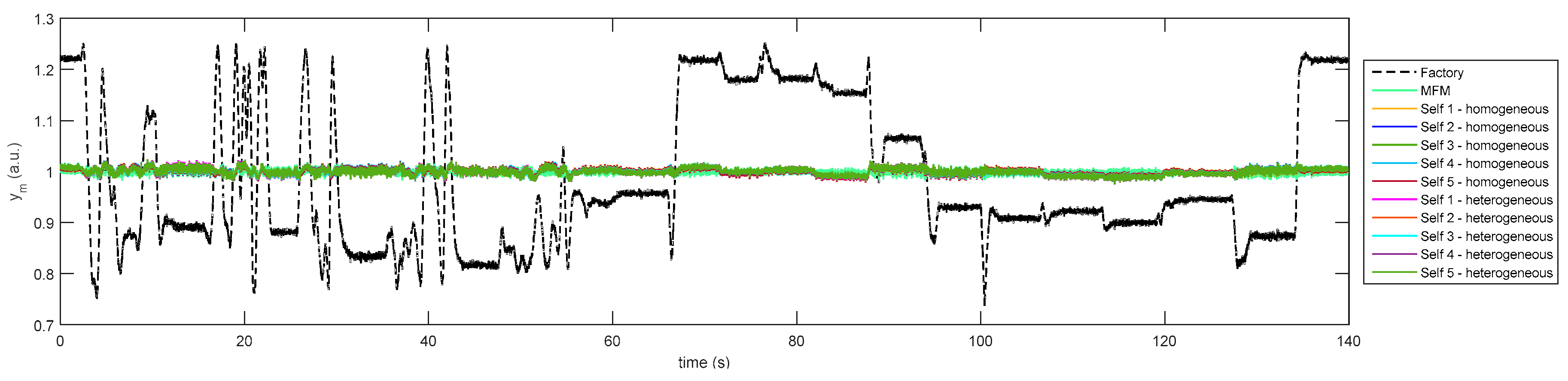
To further assess the quality of the magnetometer calibration, the magnitude of the calibrated magnetometer signal measured while rotating under a homogenous magnetic field is plotted in Figure 3. The factory calibration is not valid because the MTi-300 was mounted close to other magnetic objects during testing. The self-calibration results are consistent and show performance similar to Xsens’ Magnetic Field Mapper (MFM), which calibrates the magnetometer using the sphere-fitting approach [43]. 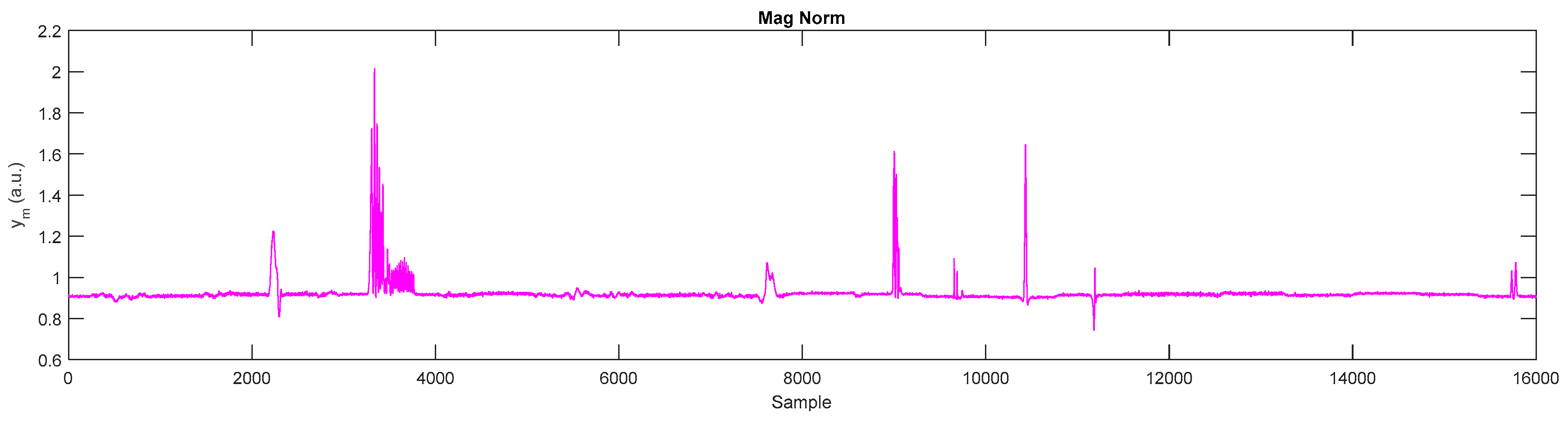Figure 4 shows the magnitude of the calibrated magnetic field measurements used in self-calibration from one of the heterogeneous magnetic field trials and demonstrate the method’s robustness to unexpected disturbances. These magnetic outliers were detected and rejected by the self-calibration method automatically and did not impact the calibration significantly. Based on the authors’ experience, the proposed gyroscope and magnetometer update, which only assumes a local constant homogenous magnetic field, has shown to yield the same calibration results as assuming a global constant homogenous magnetic field. The benefit of the proposed approach is that, under magnetic disturbances, separate clusters of local magnetic homogeneity can be automatically detected in the optimizer and can contribute to the self-calibration. Under the global homogenous field assumption, some local homogenous magnetic fields (that happen to be different from the global field) may be rejected by the outlier detector.

5.2. Case 2: On-Site User Self-Calibration

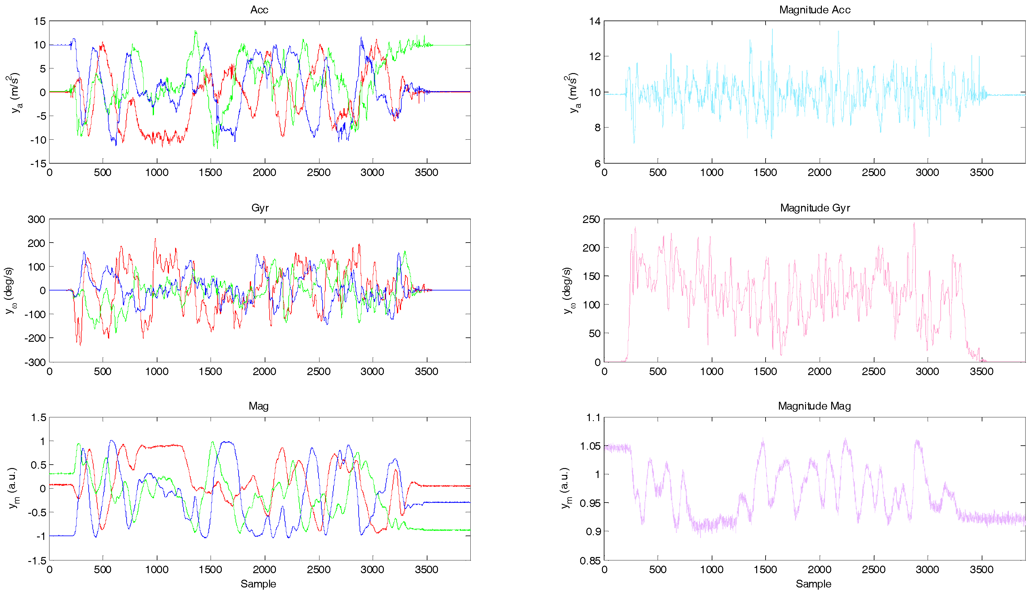
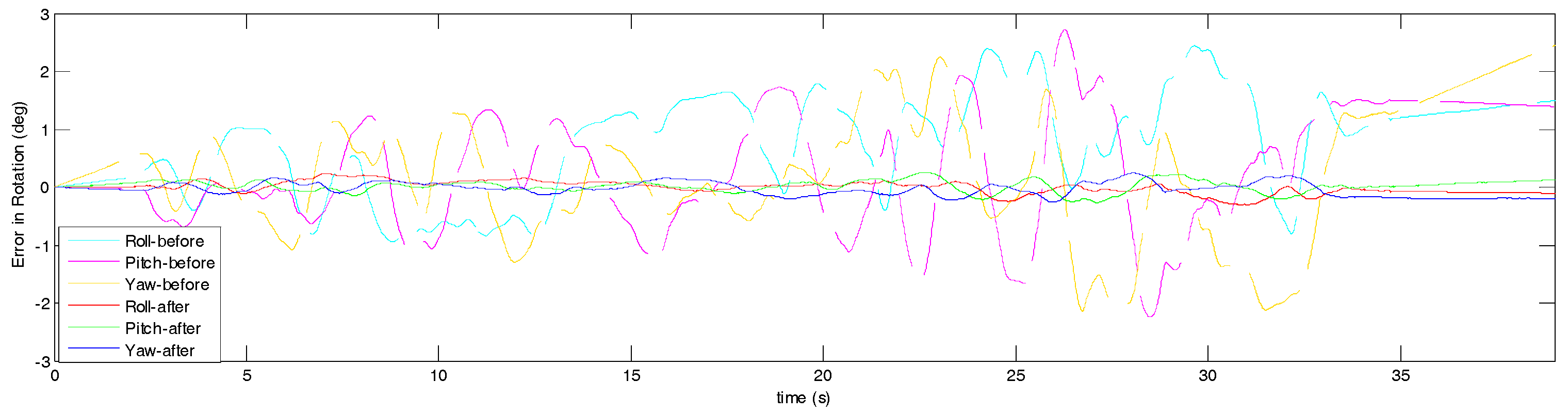
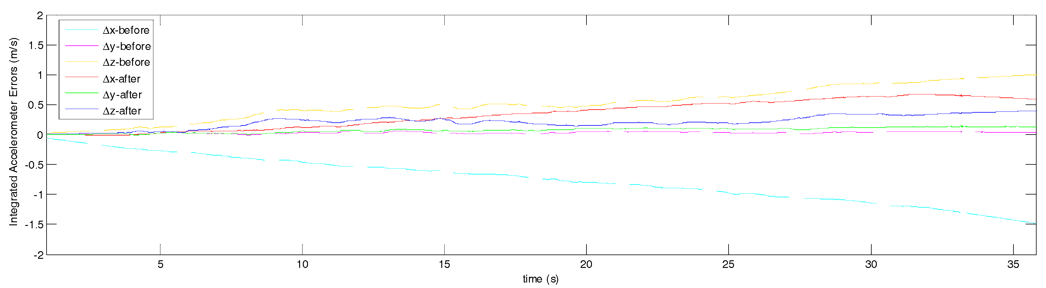
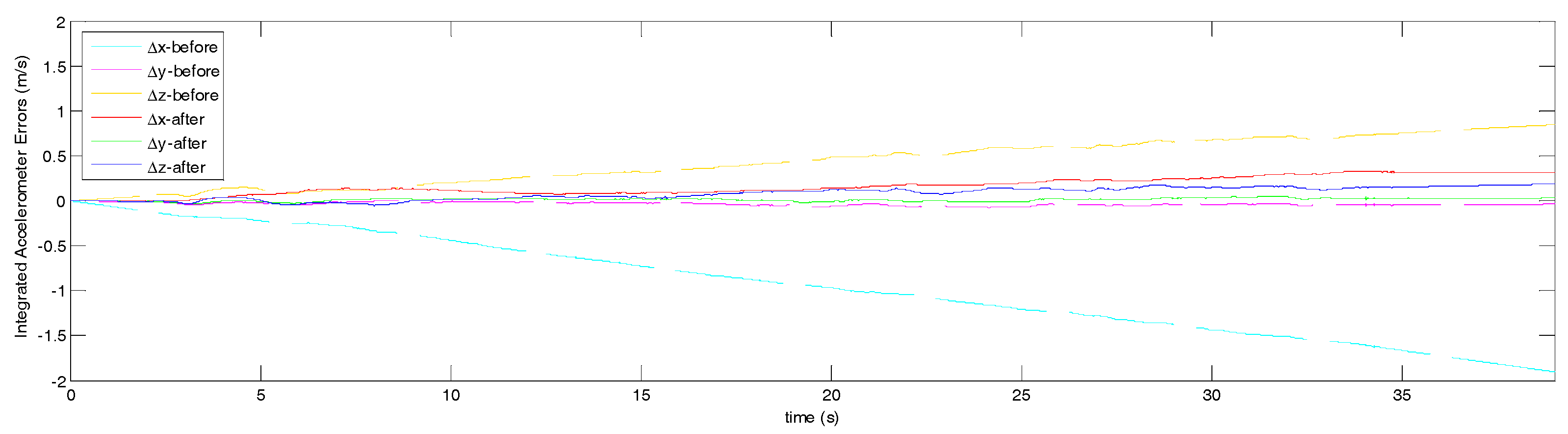
The measured accelerometer, gyroscope, and magnetometer signal from the MTi-G-700 before self-calibration is shown in Figure 5. The integrated accelerometer and gyroscope errors before and after applying the self-calibration parameters in-sample are shown in Figure 6 and Figure 7, respectively; please note that dashed lines in the cyan-magenta-yellow (CMY) color palette indicate x, y, and z errors before user self-calibration and their complementary colors in the red-green-blue (RGB) color palette with solid lines represent x, y, and z errors after user self-calibration, respectively. Noticeable reduction in errors can be perceived even after a few seconds of integration. Instead of reaching absolute errors of 2 m/s and 1.9 deg when integrating the factory calibrated inertial signals, errors well below 0.4 m/s and 0.2 deg were achieved using the new set of calibration parameters.

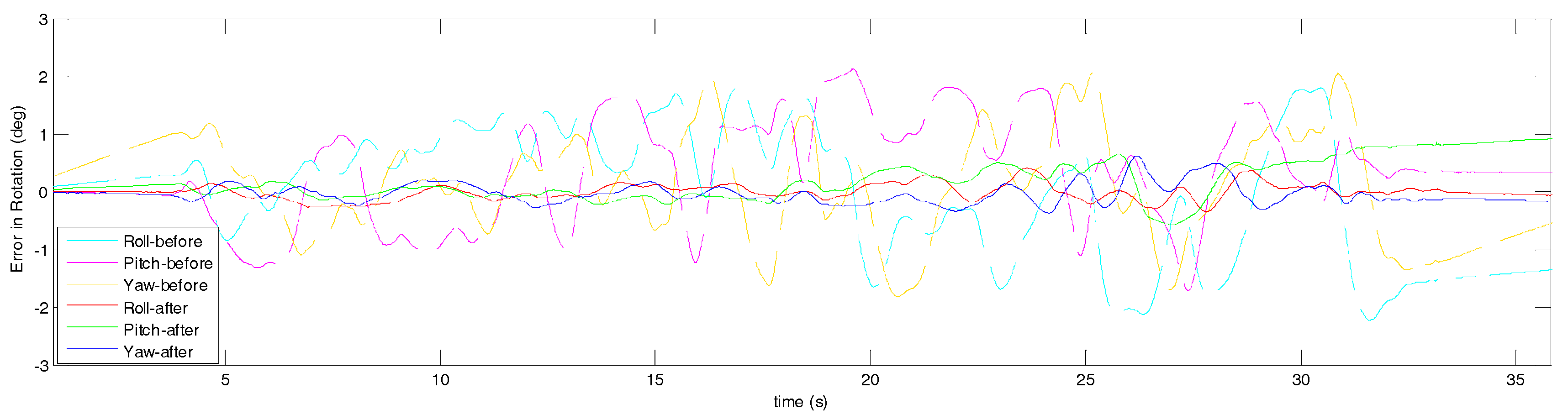
Immediately after performing the calibration, another trial was captured where the sensor was rotated freely and the navigation states were determined using the previously determined calibration parameters. The accumulated change in velocity and orientation errors of this trial (out-of-sample) are shown in Figure 8 and Figure 9. It can be perceived from the figures that after performing user self-calibration the navigation solution out-of-sample were improved.

Table 5. In-sample and out-of-sample RMSE of the input signals and estimated navigation quantities before and after on-site user self-calibration.

	In-Sample Error			Out-of-Sample Error
	Before	After	% Improv.	Before	After	% Improv.
Acceleration (m/s2)	0.09	0.09	5.33	0.09	0.08	5.34
Angular Rate (deg/s)	0.21	0.14	35.38	0.21	0.15	28.11
Integrated Acceleration (m/s)	1.19	0.22	81.62	1.26	0.52	58.47
Orientation (deg)	1.11	0.11	90.18	0.98	0.26	73.46
Velocity @ 10s (m/s)	0.76	0.20	73.33	1.96	0.15	92.13
Position @ 10s (m)	2.88	0.90	68.70	7.38	0.25	96.61

quantifies the errors for both trials before and after applying the user self-calibration parameters. On-site self-calibration was capable of improving the accuracy of the accelerometer and gyroscope signal by approximately 5% and 30%, respectively. This results in decimeter-level positioning accuracy after 10 s of dead-reckoning, and sub-degree RMSE in orientation overall. More data could have yielded a better calibration for the MTi-G-700 but there is trade-off with convenience.

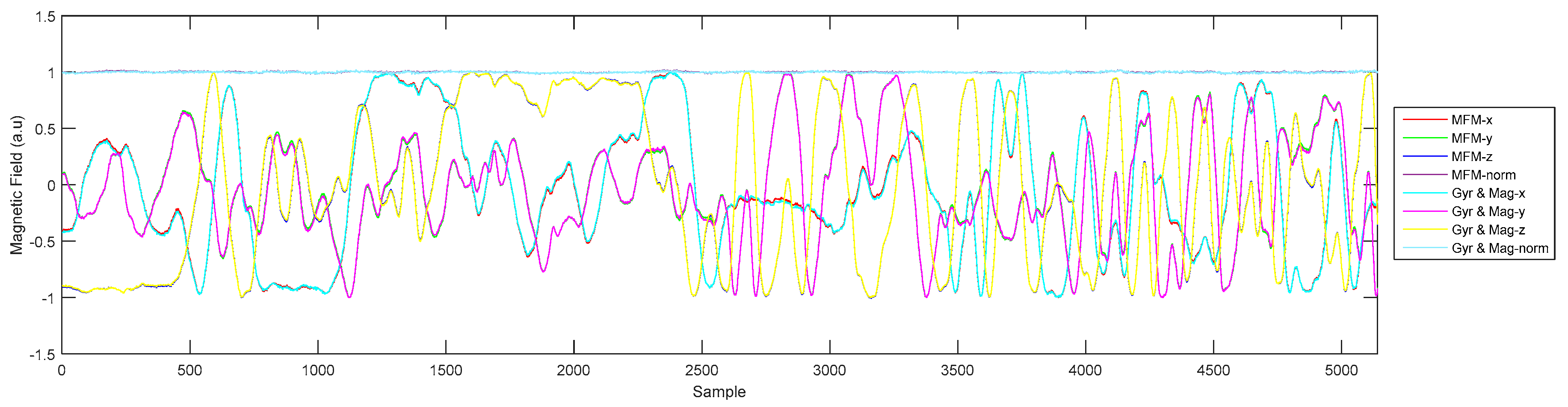
Gyroscope and Magnetometer Calibration (Accelerometer-Free Calibration)

In situations where the IMU does not stop moving or moves erratically (e.g., continuous high-dynamic movements), the gravity signal cannot be separated from the acceleration signal, therefore it becomes difficult to incorporate acceleration information into the self-calibration. However, the gyroscope and magnetometer can still be calibrated jointly using the proposed method in the absence of stillness (only Equations (6) and (7) will be active). A comparison between the manufacturer’s MFM calibration and the proposed calibration for on-site application is presented in Figure 10. The RMSE between the two signals is 0.01 a.u. for the individual x, y, and z channels. For most practical applications, the two sets of magnetometer results can be considered comparable. The main advantage of the proposed method compared to MFM are the freedom to accelerate (i.e., rotate quickly during data capture) because acceleration is not used for resolving the vertical direction and the gyroscope is calibrated simultaneously, therefore the gyroscope dead-reckoning solution can also be improved during this process. The out-of-sample rotation errors observed when using the factory calibration, manual calibration, and gyroscope and magnetometer self-calibration parameters are summarized in

Table 6. Out-of-sample RMSE for gyroscope signal and integrated angular rate in on-site self-calibration using only the gyroscope and magnetometer.

	Factory Calibration	Manual Calibration	Self-Calibration
ωx (deg/s)	0.41	0.37	0.37
ωy (deg/s)	0.23	0.19	0.21
ωz (deg/s)	0.19	0.18	0.19
Roll (deg)	2.87	0.55	0.54
Pitch (deg)	2.57	0.63	0.91
Yaw (deg)	1.81	0.42	0.81

. The proposed calibration appeared to be slightly worse than the manual calibration, but is nevertheless a significant improvement over the factory calibration results in all three principal directions and can be performed without additional equipment.

6. Conclusions

The utilization and variety of UAVs for both commercial and consumer applications are rising. Although there is a lot of diversity in the architecture of the UAVs they all use an IMU for attitude feedback control. Most of the time because of the cost, payload, and power restrictions a MEMS-based IMU is adopted. Sensor calibration can add tremendous value to MEMS IMUs but it is a time-consuming and expensive quality assurance procedure that may need to be updated frequently. This paper presented a new total-system user self-calibration routine for a 9-DoF MEMS IMU. In contrast to calibrating the individual components separately, all sensors were jointly estimated to take advantage of their correlations. It encompasses static and dynamic inertial and magnetic information and applies AUPT, CUPT, and ZUPT without external equipment to estimate the calibration parameters in post-processing. The method can enhance the quality of laboratory calibration and/or reduce this laborious process. Unlike the popular multi-position calibration method, it can recover up to 42 systematic errors simultaneously (including gyroscope scale errors, which was previously unobservable). This self-calibration method was designed to be robust against inhomogeneity in the ambient magnetic field. Results have shown that the calibration quality does not deteriorate significantly in the presence of magnetic disturbances. It is a suitable method for on-site self-calibration—for example it can be performed in tens of seconds prior to data acquisition and results have shown that dead-reckoning orientation error of 0.26 degrees over about half a minute is achievable. In the absence of useful accelerometer information, the gyroscope and magnetometer can still be calibrated simultaneously using the proposed method. This is a significant improvement over the manufacturer’s current on-site magnetometer self-calibration approach (i.e., Xsens’ MFM) because the sensor does not need to be moved slowly (simplifies data acquisition) and accuracy of the gyroscope model can also be improved, which means the strap-down integration error can be reduced. Future work will focus on a near real-time implementation of this self-calibration method for in-use applications.