Effects of Key Properties of Rainfall Series on Hydrologic Design of Sustainable Urban Drainage Systems (SUDS) ^†

Abstract

The aims of this study are to quantify the effects of key properties of rainfall time series on the hydrologic design of sustainable urban drainage systems (SUDS) to test a method for their estimation from daily time series and to quantify their uncertainty. Several typologies of SUDS infrastructures are designed to achieve a target treatment capacity. This target capacity is usually defined according to two methods: treating a percentage of the total volume of rainfall (50, 80, 90, 95, 99%) or treating a percentage of the total number of rainfall events (50, 80, 90, 95, 99%). We considered the city of Madrid as the case study, compiling 58 years of observed data (10-minutetime step) and aggregating to daily time series. We obtained the design parameters from the full resolution dataset and for different storm thresholds (0, 1 and 2 mm). Second, we determined the design parameters from the aggregated daily time series by applying a temporal stochastic rainfall generator model (RainSimV3). Finally, we estimated the model parameters from daily data and generated 100 series of 58 years at 10-minute time step, then compared the results. Results showed a good agreement compared to the 10-minute time step rainfall series. The different thresholds selected do not affect in a relevant way the calculation by percentage of the total volume; in the case of calculation by events, the threshold can vary the design volume for up to 30%. Further research includes the analysis of different climate locations.

1. Introduction

Currently, more than half of the world population lives in urban areas and growth is expected [1]. Human activity on the basins induced changes on the hydrological characteristics and higher costs for the construction and maintenance of conventional drainage systems [2,3]. The design and implementation of sustainable urban drainage systems (SUDS) could contribute to mitigating this problem by reducing the runoff volume, peak flow, and outlet contaminants [4,5,6].

The design of urban drainage systems has traditionally been carried out from historical data or through design storms [7]. However, the small size of the urban watersheds and short response time make it necessary to consider the rainfall series at a sub-hourly time-step [8,9]. From a global perspective, daily time-step rainfall data is the most common available information. Different downscaling methodologies have been widely studied for urban applications [10,11], but their application to SUDS design was not fully developed [12,13,14,15,16].

In this study, the temporal disaggregation was analyzed from daily data to 10-minute resolutions based on the Neyman-Scott Rectangular Pulse Method in a single-site and by using the RainSim V.3 model [16]. The aims of this study are to quantify the effects of key properties of rainfall time series on the hydrologic design of sustainable urban drainage systems (SUDS) to test a method for their estimation from daily time series and to quantify their uncertainty.

2. Materials and Methods

We analyzed the effect of rainfall design on two types of parameters commonly used to design SUDS: (1) those that treat a percentage of the total volume of accumulated rainfall series (50,80, 90, 95, 99%, and named as V50, V80, V90, V95, V99), and (2) those that treat a percentage of the total number of rainfall events (50, 80, 90, 95, 99%, and named as N50, N80, N90, N95, N99) during the analyzed rainfall series. The methodology applied was based on the stochastic generation of 10-minute time-step rainfall series (using the RainSimV3 model). First, we obtained the SUDS design parameters from the observed 10-minute rainfall series (58 years) and from aggregated daily rainfall time series. We estimated the parameters of the RainSimV3 model from the observed daily timeseries. Third, we generated 100 series of 58 years at 10-minute time step. Fourth, we validated the Rain Sim V3 model by comparing the intensity-duration-frequency curves (IDF) and rainfall frequency curves obtained from observed and simulated time series. Fifth, we calculated the SUDS parameters. Finally, we compared and analyzed the results.

2.1. Case Study

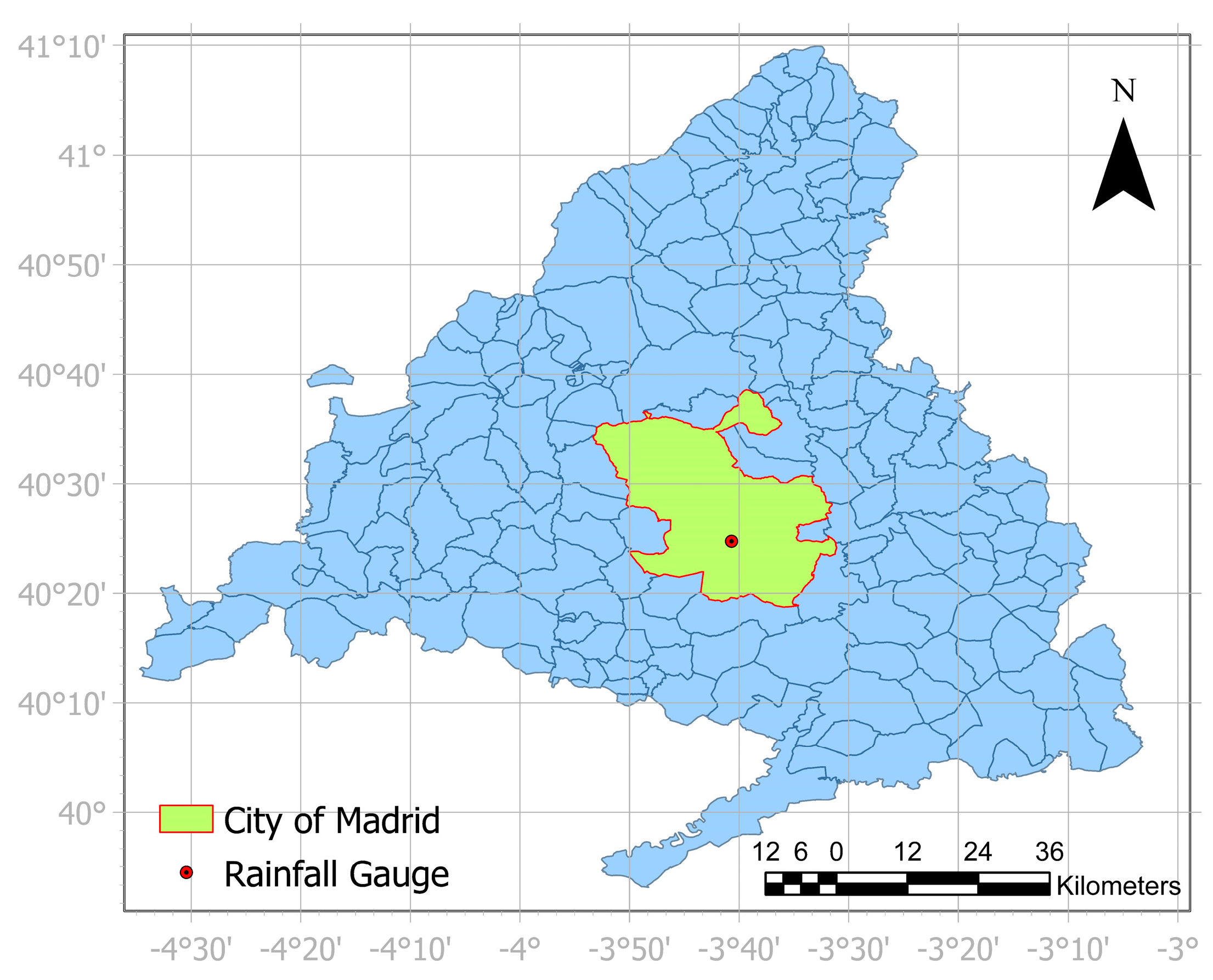
We considered the city of Madrid as the case study. We compiled 58 years of observed data (10-minute time step, from 1941 to 1998) from the Madrid Retiro gauge station (id station: 3195). Figure 1 shows the gauge location, centered on the city and located at an altitude of 667 m.a.s.l. (referred to the Alicante sea level). Madrid has a semi-arid climate with an average annual precipitation of 441 mm. The pluviography measurement series has a minimum appreciation of 0.2 mm. By aggregation, the daily data was been obtained.

2.2. Stochastic Rainfall Generation

The methodology applied was based on the stochastic generation of 10-minute time-step rainfall series by using the RainSimV3 model. First, we estimated the parameters of the RainSimV3 model from the observed daily time series. Second, we generated 100 series of 58 years at 10-minute timestep. Third, we validated the model by comparing (a) the intensity-duration-frequency curves (IDF) obtained by the model and from observed data and from previous studies [17,18,19,20,21], and (b) the rainfall frequency curves obtained from observed and simulated time series and by accounting for different storm durations (10 min, 1 h and 24 h.)

2.3. Estimation of Design Parameters (SUDS)

To estimate the SUDS parameters, we first identified the storms from the rainfall series. As usually the available rainfall series are daily time-step, and the minimum inter-storm period considered is a day [22], we assumed independent storms with a minimum inter-storm period of 24 h. We obtained the SUDS design parameters from the observed 10-minute rainfall series (58 years) and from the aggregated daily rainfall time series. We calculated the design parameters for different storm thresholds (0, 1, and 2 mm); that is, by considering all identified storms (threshold = 0 mm), by considering the storms with a total depth higher than 1 mm and 2 mm, respectively. For each storm threshold, we generated 100 series of 58 years at 10-minute time step and calculated the SUDS parameters. Finally, we compared and analyzed the results.

3. Results and Discussion

3.1. Stochastic Rainfall Validation

Table 1. Comparison of IDF curves according to different sources of data and the methods applied. Dur correspond to the storm duration in minutes and Tr the return period in years. Values are presented in mm/h.

	Observed IDF Curve				Simulated IDF Curve				AEMET (2003)				Casas-Castillo et al. (2016)				5.2-IC RETIRO (MAXPLU)
Dur/Tr	2	5	10	15	2	5	10	15	2	5	10	15	2	5	10	15	2	5	10	15
10	35.6	49.8	59.6	65.5	37.8	55.2	67.8	74.4	34.0	52.0	65.0	71.3	38.6	55.5	68.3	75.7	35.7	47.6	55.2	59.6
20	23.7	37.0	45.1	49.3	27.3	40.5	50.7	56.4	26.0	38.0	48.0	52.3	25.5	36.6	45.0	49.9	25.2	33.6	38.9	42.0
30	19.1	27.7	37.3	38.2	20.6	30.0	37.2	41.8	20.0	30.0	38.0	41.7	19.6	28.1	34.6	38.4	20.3	27.1	31.4	33.8
60	11.6	17.7	20.3	22.0	12.6	17.8	21.5	23.9	12.5	18.0	22.2	24.1	12.2	17.5	21.6	23.9	13.8	18.3	21.3	22.9
120	7.5	10.7	12.8	16.1	7.1	10.0	12.2	13.5	7.9	10.9	13.0	14.0	7.5	10.8	13.2	14.7	9.1	12.1	14.0	15.1
360	3.8	4.8	5.3	6.0	3.3	4.4	5.1	5.5	3.8	5.0	5.9	6.3	3.4	4.9	6.0	6.7	4.4	5.8	6.8	7.3
720	2.3	3.0	3.3	3.5	2.2	2.8	3.3	3.6	2.4	3.1	3.6	3.8	2.1	3.0	3.6	4.0	2.7	3.5	4.1	4.4
1440	1.4	1.8	2.2	2.3	1.4	1.8	2.1	2.3	1.5	1.9	2.2	2.3	1.2	1.8	2.2	2.4	1.6	2.1	2.4	2.6
10	Comparative Value[%] $100·\frac{(Comp..-Observed)}{Observed}$				6.1	10.9	13.7	13.5	−4.6	4.5	9.0	8.8	8.3	11.5	14.5	15.5	0.2	−4.4	−7.4	−9.1
20					15.3	9.4	12.3	14.3	9.8	2.7	6.3	6.0	7.7	−1.1	−0.3	1.1	6.4	−9.2	−13.8	−14.9
30					8.0	8.4	−0.4	9.3	4.9	8.4	1.7	9.0	2.8	1.6	−7.4	0.4	6.5	−2.0	−15.9	−11.6
60					8.9	0.6	5.9	8.4	8.0	1.8	9.3	9.3	5.4	−1.1	6.4	8.4	19.3	3.5	4.9	3.9
120					−4.9	−6.5	−4.4	−16.7	5.8	2.0	1.9	−13.3	0.5	1.0	3.4	−8.9	21.9	13.2	9.7	−6.4
360					−12.6	−9.7	−3.1	−8.8	−0.3	3.3	12.1	4.5	−10.8	1.3	14.0	11.1	15.4	19.9	29.2	21.0
720					−4.8	−5.6	−0.6	2.3	4.7	3.3	7.6	8.0	−8.4	0.0	7.6	13.6	17.8	16.6	22.5	25.0
1440					0.0	0.0	−4.2	0.0	7.1	5.6	0.6	0.0	−14.3	0.0	2.2	4.3	14.3	16.7	9.7	13.0

shows the values of the IDF curves obtained from the observed 10-minute time-series, the simulated series, and previous studies. Casas-Castillo et al. [17] used 5-minute rainfall series from1940 to 2012. AEMET [18] obtained the IDF curves by fitting the observed data (10-minute series from1942 to 2002) to a SQRT-ETmax. Distribution function [23]. Finally, results from the application of the national 5.2IC [19] are shown (rainfall values were extracted from the MAXPLU study [20]. Results show that the median values from the stochastic simulations (with parameters adjusted using observed daily data) have a good agreement compared with the results from the 10-minute data, with differences smaller than 10% for most of the analyzed storm durations and return periods. Moreover, the differences are within the 95% confidence interval estimated by the stochastic simulations.

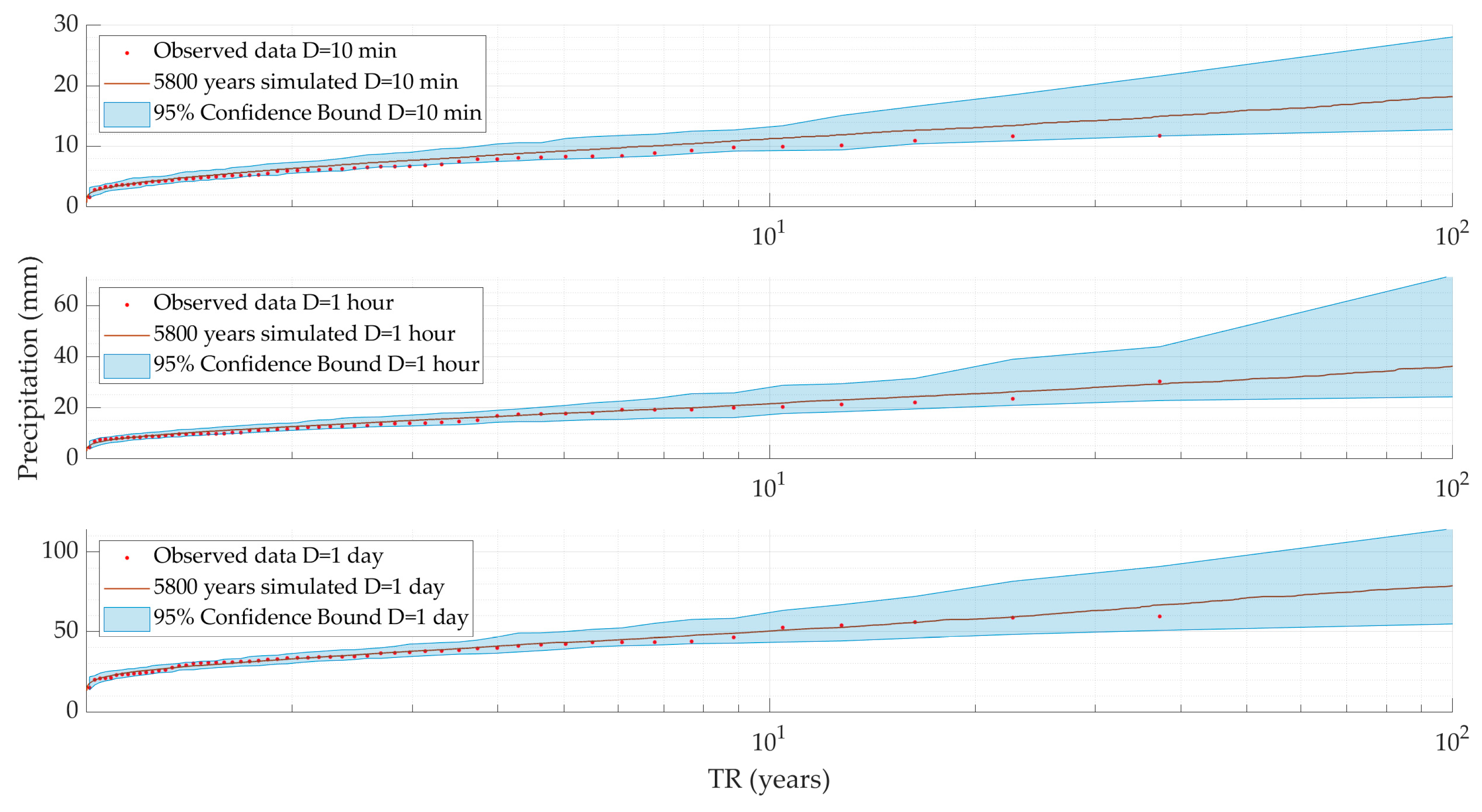
Figure 2 shows the rainfall frequency curves (RFC) corresponding to rainfall durations of 10 min, 1 h and 24 h respectively. Simulated RFC curves for 1 h and 24 h show an excellent agreement compared with their correspondent observed RFC curves (calculated from 10-minute time series). It should be noted that the simulated RFC curves were generated with parameters estimated from daily data. Thus, the proposed stochastic procedure has a good predictive capacity for extreme value estimation.

3.2. Design Parameters Analysis (SUDS)

3.2.1. Parameters Based on Rainfall Volume

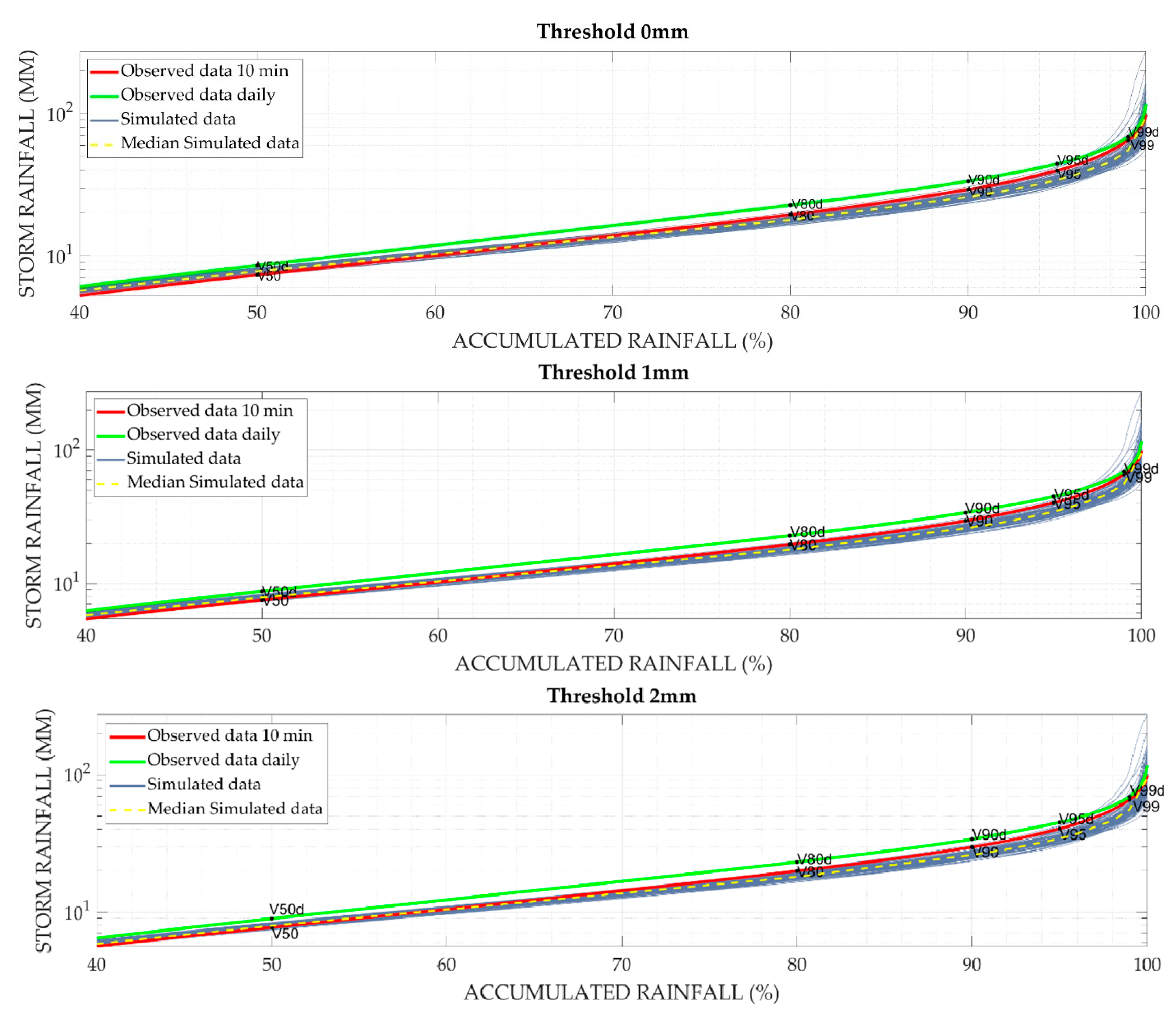
Figure 3 and

Table 2. Comparison of the SUDS design values (V50, V80, V90, V95 and V99) in mm. by using the10-minute observed data, daily observed data and stochastic generated data, and by considering different storm thresholds (0, 1 and 2 mm).

	Observed 10 min	Observed Daily	Simulated		Error Daily	Error Simulated
			Min	Max	Median	%	%
Threshold 0 mm
V50	7.35	8.57	7.23	8.25	7.8	17%	6%
V80	19.53	22.89	16.4	20.3	18	17%	−8%
V90	29.39	33.64	23.4	30.8	26.15	14%	−11%
V95	40.17	44.81	30	42.9	34.5	12%	−14%
V99	65.38	69.94	44.7	112.5	57.25	7%	−12%
Threshold 1 mm
V50	7.49	8.72	7.29	8.32	7.85	16%	5%
V80	19.78	22.96	16.5	20.4	18	16%	−9%
V90	29.6	33.93	23.5	30.9	26.2	15%	−11%
V95	40.15	44.8	30.4	42.9	34.6	12%	−14%
V99	67.55	69.93	44.7	112.5	57.25	4%	−15%
Threshold 2 mm
V50	7.75	8.95	7.41	8.41	7.96	15%	3%
V80	20	23.3	16.6	20.5	18.2	17%	−9%
V90	29.9	34.21	23.6	31.2	26.25	14%	−12%
V95	40.82	45	30.4	42.9	34.65	10%	−15%
V99	67.55	69.94	44.7	112.5	57.25	4%	−15%

shows, for the different storm thresholds considered, the values and uncertainty of the V50, V80, V80, V90, V90, V95, and V99 derived from the 100 analyzed series. In addition, values obtained from the observed 10-minute and daily time series are also plotted. Although results show better performance of the stochastic series assuming a threshold value of 2 mm compared with 1 mm and considering all events, the SUDS design parameters, for this case study, did not present high sensitivity. For V50, V80, and V90, better results were obtained for the stochastic approach than for daily data. Thus, starting from observed daily data, the stochastic approach could obtain similar SUDS design values than using observed daily data, but also estimated a 10-minute time-step series, very useful for SUDS design. For example, for a better estimation of storm characteristics as temporal distribution of storms, time among events, and maximum and mean rainfall intensities, among others. Finally, results from observed 10-minute time step are within the 95% confidence bound of the stochastic simulation.

3.2.2. Design Parameters Based on Number of Events

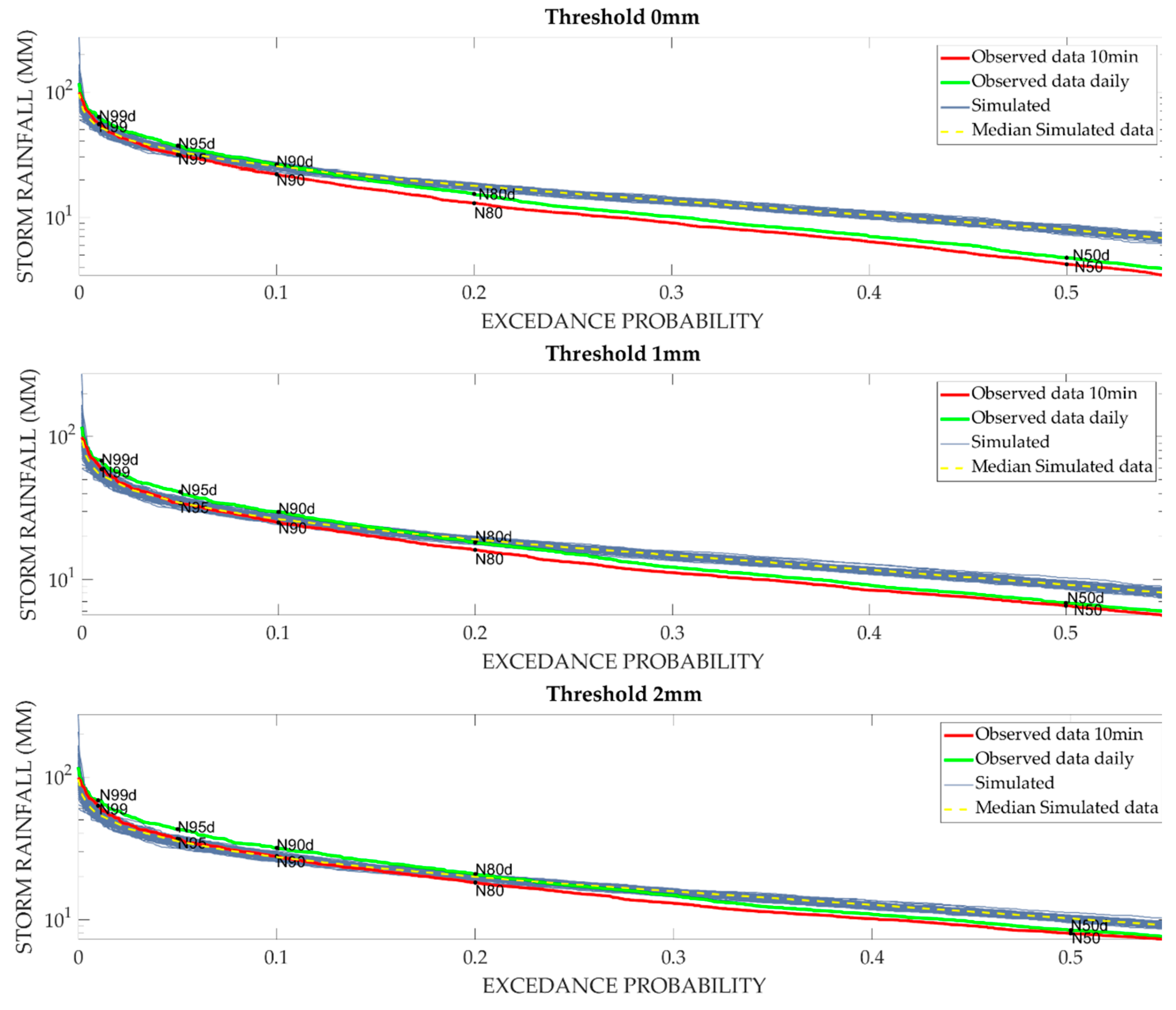
Figure 4 and

Table 3. Comparison of the SUDS design values (N50, N80, N90, N95 and N99) in mm. by using the10-minute observed data, daily observed data and stochastic generated data, and by considering different storm thresholds (0, 1 and 2 mm).

	Observed 10 min	Observed Daily	Simulated			Error Daily %	Error Simulated %
			Min	Max	Median
Threshold 0 mm
N50	4.2	4.75	7.2	8.8	8	13%	90%
N80	13.03	15.42	16.4	19	17.9	18%	37%
N90	22.15	26.1	23.13	27.32	25.35	18%	14%
N95	31.29	37	29.9	36.48	33.11	18%	6%
N99	55.02	62.83	46.19	63.19	52.4	14%	−5%
Threshold 1 mm
N50	6.54	6.85	8.5	10.3	9.2	5%	41%
N80	16.09	18.15	17.5	20.02	19.07	13%	19%
N90	25.07	29.63	24.13	28.88	26.4	18%	5%
N95	34.12	40.9	30.55	38.07	34.3	20%	1%
N99	59.015	67.67	47.91	66.029	53.6	15%	−9%
Threshold 2 mm
N50	8	8.42	9.5	11.2	10.2	5%	28%
N80	18.18	20.84	18.5	21	20	15%	10%
N90	27.82	31.77	25.3	30.3	27.45	14%	−1%
N95	36.8	43.05	31.5	39.2	35.45	17%	−4%
N99	62.84	68.6	48.3	69.95	57.76	9%	−8%

show, for the different storm thresholds considered, the values and uncertainty of the N50, N80, N90, N95, and N99 derived from the 100 analyzed series. In addition, values obtained from the observed 10-minute and daily time series are also presented. Results show a good performance of the simulated N80, N90, N95, and N99 by considering a storm threshold of 2 mm. For design parameters based on the number of identified events, both the storm threshold considered and the criteria adopted to identify independent storms affect results significantly. For N80, N90, N95, and N99, better results were obtained for the stochastic approach than for daily data (storm threshold = 2 mm).

4. Conclusions

The use of a stochastic approach for the generation of 10-minute time step rainfall series from daily observed data showed a good agreement compared to the 10-minute time step rainfall series. The proposed approach allows the estimation of very useful rainfall characteristics for SUDS design as the temporal distribution of storms, time among events, maximum, and mean storm rainfall intensities, among others. For the case study analyzed, the stochastic approach generated 10-minute rainfall series with IDF curves, and rainfall frequency curves similar to observed data. Parameters to design SUDS based on the number of storms identified have more dependence on the criteria, adopted to define independent storms or the minimum value of rainfall to consider a storm. However, the parameters to design SUDS based on the volume of the storm events are not sensible to the mentioned criteria. This approach allows us to quantify the associated uncertainty of the values adopted to the design of SUDS. It should be noted that we applied this methodology to one location. This might limit the generalization of the results obtained. Further research will be focused on the application of this approach on locations with different climate characteristics.

References

- United Nations. World Urbanization Prospects: The 2011 Revision; United Nations Department of Economic and Social Affairs (Population Division): New York, NY, USA, 2011. [Google Scholar]
- Hair, L.; Clements, J.; Pratt, J. Insights on the Economics of Green Infrastructure: A Case Study Approach. In Proceedings of the Water Environment Federatio. WEFTEC 2014: Session 310 through Session 317, New Orleans, LA, USA, 27 September–1 October 2014; pp. 5556–5585. [Google Scholar] [CrossRef]
- Sordo-Ward, A.; Bianucci, P.; Garrote, L.; Granados, A. How safe is hydrologic infrastructure design? Analysis of factors affecting extreme flood estimation. J. Hydrol. Eng. 2014, 19, 04014028. [Google Scholar] [CrossRef]
- Arora, A.S.; Reddy, A.S. Multivariate analysis for assessing the quality of stormwater from different urban surfaces of the Patiala City, Punjab (India). Urban Water J. 2013, 10, 422–433. [Google Scholar] [CrossRef]
- Hatt, B.E.; Fletcher, T.D.; Walsh, C.J.; Taylor, S.L. The influence of urban density and drainage infrastructure on the concentrations and loads of pollutants in small streams. Environ. Manag. 2004, 34, 112–124. [Google Scholar] [CrossRef] [PubMed]
- Woods-Ballard, B.; Wilson, S.; Udale-Clarke, H.; Illman, S.; Scott, T.; Ashley, R.; Kellagher, R. The SUDS Manual, C753; Ciria: London, UK, 2015. [Google Scholar]
- Mikkelsen, P.S.; Madsen, H.K.; Arnbjerg-Nielsen, K.; Jørgensen, H.K.; Rosbjerg, D.; Harremoës, P. A rationale for using local and regional point rainfall data for design and analysis of urban storm drainage systems. Water Sci. Technol. 1998, 37, 7–14. [Google Scholar] [CrossRef]
- Bennett, N.D.; Croke, B.F.W.; Guariso, G.; Guillaume, J.H.A.; Hamilton, S.H.; Jakeman, A.J.; Marsili-Libelli, S.; Newham, L.T.H.; Norton, J.P.; Perrin, C.; et al. Characterising performance of environmental models. Environ. Model. Softw. 2013, 40, 1–20. [Google Scholar] [CrossRef]
- Cowpertwait, P.S. A spatial-temporal point process model of rainfall for the Thames catchment, UK. J. Hydrol. 2006, 330, 586–595. [Google Scholar] [CrossRef]
- Rodriguez-iturbe, I.; Depower, B.F.; Valdes, J.B. Rectangular pulses point process models for rainfall: Analysis of empirical data. J. Geophys. Res. Atmos. 1987, 92, 9645–9656. [Google Scholar] [CrossRef]
- Entekhabi, D.; Rodriguez-Iturbe, I.; Eagleson, P.S. Probabilistic representation of the temporal rainfall process by a modified Neyman-Scott rectangular pulses model—Parameter-estimation and validation. Water Resour. Res. 1989, 25, 295–302. [Google Scholar] [CrossRef]
- Paschalis, A.; Fatichi, S.; Molnar, P.; Rimkus, S.; Burlando, P. On the effects of small scale space-time variability of rainfall on basin flood response. J. Hydrol. 2014, 514, 313–327. [Google Scholar] [CrossRef]
- Kaczmarska, J.; Isham, V.; Onof, C. Point process models for fine-resolution rainfall. Hydrol. Sci. J. 2014, 59, 1972–1991. [Google Scholar] [CrossRef]
- Khaliq, M.N.; Cunnane, C. Modelling point rainfall occurrences with the Modified Bartlett-Lewis Rectangular Pulses Model. J. Hydrol. 1996, 180, 109–138. [Google Scholar] [CrossRef]
- Burton, A.; Kilsby, C.G.; Fowler, H.J.; Cowpertwait, P.S.P.; O’Connell, P.E. RainSim: A spatial-temporal stochastic rainfall modelling system. Environ. Model. Softw. 2008, 23, 1356–1369. [Google Scholar] [CrossRef]
- Cowpertwait, P.S.P. A spatial-temporal point process model with a continuous distribution of storm types. Water Resour. Res. 2010, 46, W12507. [Google Scholar] [CrossRef]
- Casas-Castillo, M.C.; Rodriguez-Sola, R.; Navarro, X.; Russo, B.; Lastra, A.; Gonzalez, P.; Redano, A. On the consideration of scaling properties of extreme rainfall in Madrid (Spain) for developing a generalized intensity-duration-frequency equation and assessing probable maximum precipitation estimates. Theor. Appl. Climatol. 2018, 131, 573–580. [Google Scholar] [CrossRef]
- INM (AEMET). Curvas de Intensidad–Duración–Frecuencia. [CD, Recurso Electrónico]; Ministerio de Medio Ambiente: Madrid, Spain, 2003. [Google Scholar]
- Ministerio de Fomento. Instrucción de Carreteras 5.2-IC Drenaje Superficial; Dirección General de Carreteras; Ministerio de Fomento: Madrid, Spain, 2016. (In Spanish) [Google Scholar]
- Ministerio de Fomento. Máximas Lluvias Diarias en la España Peninsular; Dirección General de Carreteras; Ministerio de Fomento: Madrid, Spain, 1999. (In Spanish) [Google Scholar]
- Sordo-Ward, A.; Bianucci, P.; Garrote, L.; Granados, A. The influence of the annual number of storms on the derivation of the flood frequency curve through event-based simulation. Water 2016, 8, 335. [Google Scholar] [CrossRef]
- Stormwater Management Manual. City of Portland. 2016. Available online: https://www.portlandoregon.gov/bes/64040 (accessed on 15 August 2018).
- Etoh, T.; Murota, A.; Nakanishi, M. SQRT-Exponential Type Distribution of Maximum. In Proceedings of the International Symposium on Flood Frequency and Risk Analyses, Louisiana State University, Baton Rouge, LA, USA, 14–17 May 1986; Shing, V.P., Ed.; Reidel Publishing Company: Boston, MA, USA, 1987; pp. 253–264. [Google Scholar]
Figure 1.
Location of the study case. Red dot indicates the rainfall gauge location.
Figure 2.
Comparison of the estimated rainfall frequency curves corresponding to 10-minute storm duration (D, red dots), 1 h and 1 day, their corresponding stochastic simulation (red line), and 95% confidence bound (cyan area).
Figure 3.
Comparison of the SUDS parameters based on rainfall event volumes. Red line represents the event rainfall volume value that ensure a treatment of the 50, 80, 90, 95, and 99% of the accumulated rainfall depth within the analyzed period (58 years) at 10-minute time step. Green line corresponds to daily time step, blue lines correspond to the stochastic simulations at 10-minute timestep, and yellow dotted line represent the median values of the stochastic simulation.
Figure 4.
Comparison of the SUDS parameters based on the number of rainfall events. Red line represents the event rainfall volume value that ensure a treatment of the 50, 80, 90, 95 and 99% of the total storm events within the analyzed period (58 years) at 10-minute time step. Green line corresponds to daily time step, blue lines correspond to the stochastic simulations at 10-minute timestep and yellow dotted line represent the median values of the stochastic simulation.