Integral Sliding Mode Backstepping Control of an Asymmetric Electro-Hydrostatic Actuator Based on Extended State Observer ^†

Abstract

To provide high output force and to reduce the installation space, the electro-hydrostatic actuator (EHA) usually adopts asymmetric cylinder. However, comprehensive effects produced by its asymmetric flow, parameter uncertainties and unknown disturbance make it difficult to achieve high-accuracy position control. This paper proposed an integral sliding mode backstepping control (ISMBC) based on extended state observer for the asymmetric EHA. Firstly, the principle of the EHA was analyzed and an EHA model was built. Furthermore, the state space equation of the EHA was established based on flow distribution analysis. Two extended state observers (ESO) were designed to achieve real-time estimation of the unmeasured system states, unmatched and matched disturbances. The backstepping method was used to compensate the matched and unmatched disturbance, and an integrated sliding mode controller was developed to eliminate the static error and to improve the response ability. Theoretical analysis indicates that the controller can guarantee the desired tracking performance for the actuator under time-varying unmatched disturbances, and can make the tracking error asymptotically converge to zero under constant matched disturbances. Finally, simulations were performed with the designed controller, backstepping controller and proportional–integral–derivative (PID) controller, respectively. Thereafter, detailed comparisons of the control performances were provided. The results show that the proposed controller can achieve better position tracking and stronger robustness in parameter changing compared with the backstepping controller and PID controller.

1. Introduction

Electro-hydrostatic actuators (EHAs) are widely used in aviation, shipbuilding, automobile and other industrial fields due to their small size, light weight, high efficiency and great reliability [1,2,3]. The EHA is a highly integrated direct driven hydraulic system that integrates an electric motor, a pump, an actuator, a tank, etc. [1,4]. It achieves variable power transmission of actuators by changing the rotation speed or the displacement of the pump [5]. Compared with the traditional valve-controlled system, the EHA eliminates the throttling loss caused by the multi-way valve and the overflow loss caused by the centralized oil supplies, which significantly improves the system efficiency [6,7].

Over the past 20 years, EHAs have been applied in high-precision industries such as aviation and submarines [8,9], but only adopting actuators with symmetrical structures. However, industrial applications usually require asymmetric hydraulic actuators, having the advantages of smaller volume and larger output force [10]. The unbalanced flow in asymmetric EHAs, caused by the unequal effective cross-section areas in two chambers, seriously affects the control accuracy and dynamic response [11,12].

To solve this problem, many novel methods were proposed such as the development of asymmetric flow distribution pumps [13], the research of pump-valve-coordinated system [14] and the use of dual-pumps control system [15], and on the other hand, advanced control algorithms such as robust adaptive control [16,17,18], backstepping control and sliding mode control.

In addition, EHA has the characteristics of nonlinearities, parametric uncertainties and external disturbances [19,20,21]. These nonlinearities include fluid compressibility, nonlinear friction, internal and external leakage [22]. Parametric uncertainties are mainly caused by model inaccuracy and system parameters variation. The external disturbances mainly consist of the variation of external load force and unmodeled load force. The nonlinear friction reduces the response speed by affecting the transient characteristics of the EHA and leads to viscous and crawling phenomena in low-speed operation. Leakage in the EHA decreases steady-state accuracy. Parametric uncertainties normally require a high gain to improve the robustness of the system, which easily lead to over-design. External disturbances reduce system stability by influencing system output [23].

To solve these problems of nonlinearities, uncertainties and external disturbances, a lot of research has been conducted. Lin [24] regarded the nonlinear friction force as norm-bounded uncertainties, and developed a robust discrete-time sliding-mode control (DT-SMC) for an EHA system. Fu [25] applied neural networks to identify uncertainties online, combined RBF neural networks with fast terminal sliding mode controller, which not only solved the problem of sliding mode control depending on system parameters but also suppressed oscillation to some extent. Alemu [26] applied the extended state observer (ESO) to estimate the system states, uncertainties and external disturbances, used the friction model to compensate the friction force, and designed a sliding mode controller for the system, which improved the robustness while ensuring the tracking performance. Sun [27] developed a nonlinear robust motion controller based on the extended disturbance observer to compensate the estimation error of the outer position tracking loop, while the inner pressure control loop adopted a backstepping method to achieve accurate force control. Wang [28] introduced a feedback backstepping control algorithm based on the backstepping control theory for the high-order model of the EHA system to convert the complex nonlinear system into a linear system. Yang [29] introduced a filtered error function, and integrated a novel expected compensation adaptive control framework into the controller to reduce environmental noise. Shen [30] decomposed the 5th-order EHA dynamic model into four subsystems, and designed adaptive control laws, respectively, to solve the controller design problem of the high-order system. Yang [31] designed a linear state observer and a nonlinear disturbance observer to estimate the matched and unmatched disturbances in the system, and employed a continuously differentiable friction model to compensate the friction force.

The above research shows that combining the observer with advanced control theory is an effective method to solve the problems of nonlinearities, uncertainties and disturbances in hydraulic systems. Most scholars focus on improving the control performance of symmetric EHAs and valve-controlled systems. Therefore, this paper proposed a novel control strategy to solve the uncertainty problem of an asymmetric EHA. The electric motor speed control system was regarded as a separate module, and PI controller was adopted. The state equation of the asymmetric EHA system was established considering nonlinear friction, parameter uncertainty and external disturbance. The Stribeck static friction force model was used to identify the friction force; the unmodeled friction force was regarded as an external disturbance. The state equation was used to judge whether the disturbance and the control law were on the same channel. The disturbances were divided into matched disturbance and unmatched disturbance, two ESOs were established for estimation. The integral sliding mode algorithm was added in the first step of the backstepping design to reduce the steady-state error and to improve the robustness of the EHA. Based on the Lyapunov theory, the stability and effectiveness of this control method were proven. The simulation results show that the controller has good steady-state characteristics and high control accuracy.

The remainder of this paper is organized as follows. Section 2 presents the principal analysis and model building of an asymmetric EHA. In Section 3, two ESOs are designed to deal with the disturbances and its convergence is verified. In Section 4, the integral sliding mode backstepping control (ISMBC) controller is proposed, and its stability is proven. Section 5 gives comparative simulation results. Finally, the conclusion is given in Section 6.

2. Principal Analysis and Modelling

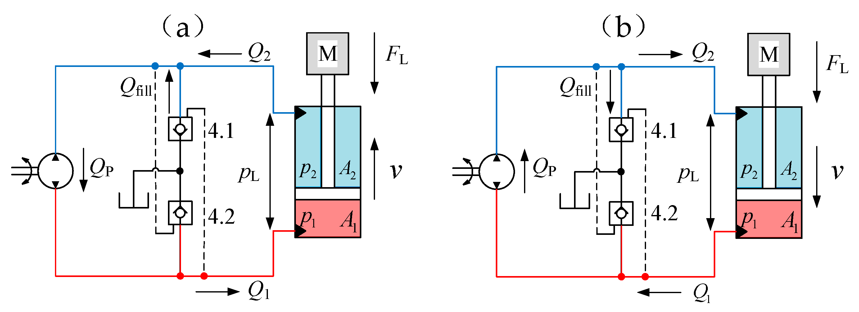
2.1. Load Force Analysis of a Micro Crane

In this case study, the research object is the micro crane, as shown in Figure 1. The dimensions of the micro-crane were measured, and its 3D model was created in Solidworks. After that, the dynamic model of the crane was built by exporting a CAD assembly from Solidworks and importing into Matlab/Simulink. The output force of the EHA system installed on the crane mainly depends on the torque, angular acceleration.

According to Newton’s second law, the torque balance equation of the boom can be written as:

$$\sum M_{\mathsf{\Theta }}=J\frac{d^2\theta }{{\mathit{dt}}^2},$$

(1)

where (d²θ)⁄dt² is the angular acceleration; J is the rotational inertia of boom.

Decomposed Equation (1) to obtain the output force equation of the hydraulic cylinder [15]

$$F_{\mathrm{Cyl}}=[J\frac{d^2\theta }{{\mathit{dt}}^2}+\mathit{mg}·r_m\sin ({\theta }_m)+m_{l}g·r_l\sin ({\theta }_l)]/d_1\sin (\alpha ),$$

(2)

where F_Cyl is the output force of cylinder; m is the mass of boom; r_m is the distance between the centre of mass and the joint; θ_m is the angle between the centre of mass and the reference coordinate vertical axis; g is gravitational acceleration; the load is connected to the crane by a hook and chain, and therefore, the load force is always perpendicular to the ground, such that m_l can be defined as load mass including the mass of load, hook and the chain; r_l is the distance from the load acting on the arm to the joint; θ_l is the angle between the connection about the joint and load with the reference coordinate vertical axis; d₁ is the distance between the cylinder base and the joint; α is the angle between the cylinder and the joint.

Next, the working principle of asymmetric EHA was analyzed, and the state-space equation was established for the EHA.

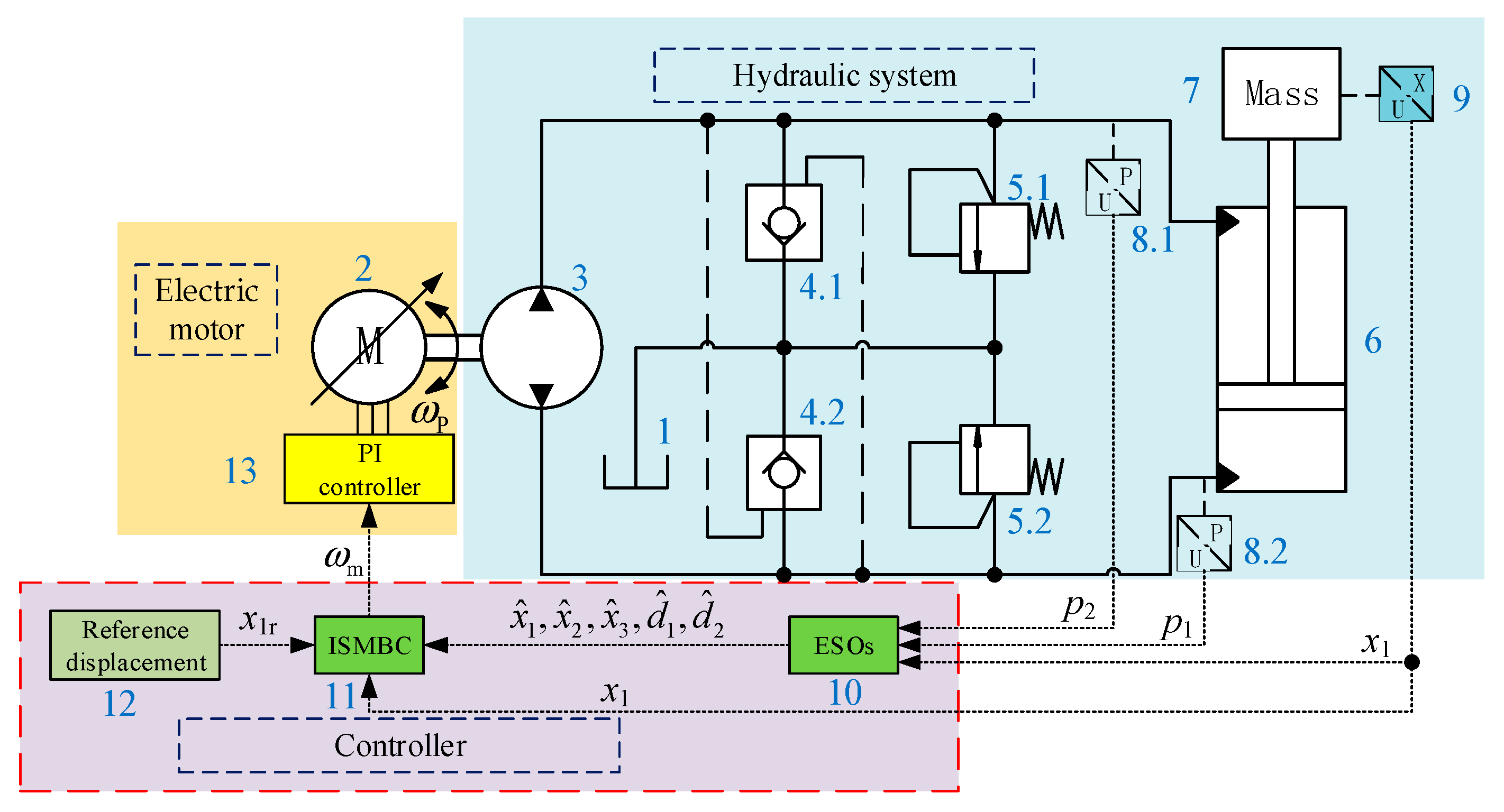
2.2. Principle Analysis of EHA

The schematic of the EHA control system is shown in Figure 2. The system includes the hydraulic system, the electric motor and the controller. The variable speed electric motor is controlled by PI controller, which drives a bidirectional fixed pump. Two pilot-operated check valves are used to balance the flow of the asymmetric cylinder. Two relief valves are used for safety purposes.

The EHA, installed on the micro-crane as shown in Figure 1, runs in two operating conditions including extending and retracting with positive load, as shown in Figure 3. Therefore, the load pressure p_L is always greater than zero; this was given by

p_L = p₁ − ap₂

(3)

where p₁ and p₂ are the pressures of the piston chamber and the rod chamber of the cylinder, respectively; a is the area ratio of cylinder, a = A₂/A₁; A₁ and A₂ are the areas of the piston chamber and the rod chamber of the cylinder, m².

Due to the different effective areas of the asymmetric cylinder, EHA requires unequal oil flow rate during moving. To prevent cavitation, hydraulic oil is replenished from the oil tank through the pilot-operated check valve 4.1, as shown in Figure 3a. During retracting, the excess oil flow from the piston chamber backs to the oil tank through the pilot-operated check valve 4.1, as shown in Figure 3b.

2.3. Modelling

2.3.1. Model of the Electric Motor

Permanent magnet synchronous motors (PMSMs) are widely used in industrial equipment because of high power density, high efficiency and high reliability. Hence, in this paper, a PMSM was selected to drive the EHA. The electromagnetic torque equation of PMSM in d-q reference frame can be expressed as

T_{E =} 1.5p_nψ_mi_sq,

(4)

where T_E is the electromagnetic torque; p_n is the number of pole pairs; ψ_m is the rotor magnet flux linkage; i_sq is the q-axis stator currents.

Assuming the PMSM rotates at a constant speed, the torque balance equation between the PMSM and the pump can be written as

$${\dot{\omega }}_{\mathrm{m}}=\frac{1}{J}(1.5p_{\mathrm{n}}{\psi }_{\mathrm{m}}{i}_{\mathrm{sq}}-B{\omega }_{\mathrm{m}}-T_{\mathrm{L}}),$$

(5)

where $J$ is the moment of inertia; $B$ is the viscous friction coefficient; $T_{\mathrm{L}}$ is the load torque from the pump; ${\omega }_m$ is the angular speed of the rotor.

In the Laplace transformation of Equation (5), ignoring the effects of the pump torque, the transfer function of the motor can be given as

$$\frac{{\omega }_{\mathrm{m}}\left(s\right)}{I_{\mathrm{sq}}\left(s\right)}=\frac{K}{\tau s-1}.$$

(6)

where $K$ is the electric motor gain,$K=1.5p_{\mathrm{n}}{\mathsf{\psi }}_{\mathrm{m}}/B$; $\tau$ is the time constant, $\tau =J/B$.

The PMSM mainly adopts $i_{\mathrm{sd}}=0$ vector control; the outer loop speed control provides a reference signal for the inner current loop. This paper focuses on designing high-precision EHA system controller, so the proportional-integral (PI) was used as a speed loop controller for the electric motor.

2.3.2. Model of the Hydraulic System

The output flow of the pump can expressed by

$$Q_{\mathrm{P}}=\frac{D_{\mathrm{P}}}{2\pi }{\omega }_{\mathrm{P}}-c_{\mathrm{i}}\Delta p,$$

(7)

where $Q_{\mathrm{P}}$ is the output flow of pump, m³/s; $D_{\mathrm{P}}$ is the pump displacement, m³/r; ${\omega }_{\mathrm{P}}$ is the pump angular speed,${\omega }_{\mathrm{P}}={\omega }_{\mathrm{m}}$, rad/s; $c_{\mathrm{i}}$ is the internal leakage coefficient, (m/s)/Pa; $\Delta p$ is the differential pressure,$\Delta p=p_1-p_2$.

Due to the pressure $p_2$ close to zero, for simplification, assuming $\Delta p\approx p_{\mathrm{L}}$, Equation (7) can be rewritten as

$$Q_{\mathrm{P}}=\frac{D_{\mathrm{P}}}{2\pi }{\omega }_{\mathrm{P}}-c_{\mathrm{i}}{p}_{\mathrm{L}}.$$

(8)

The flow-pressure equation of cylinder can be expressed as

$$\{\begin{array}{c}{Q}_{\mathrm{P}}=Q_1=A_1{\dot{x}}_{\mathrm{P}}+V_1{\dot{p}}_1/{\beta }_{\mathrm{e}} \\ -a{Q}_{\mathrm{P}}=Q_2=A_2{\dot{x}}_{\mathrm{P}}+V_2{\dot{p}}_2/{\beta }_{\mathrm{e}}\end{array},$$

(9)

where $Q_1$ and $Q_2$ are flowrates of the piston chamber and the rod chamber of the cylinder, m³/s; ${\beta }_{\mathrm{e}}$ is the effective bulk modulus, Pa; $V_1$ and $V_2$ are the current volumes of the cylinder, m³, $V_1=V_{01}+A_1{x}_{\mathrm{P}}$, $V_2=V_{02}-A_2\left(s-x_{\mathrm{P}}\right)$; $V_{01}$ and $V_{02}$ are the initial volumes of two-chambers of the cylinder; $s$ is the piston stroke, m.

Assuming that the piston is moving around the centre position, the following approximation can be given [32]:

$$\frac{V_1}{{\beta }_{\mathrm{e}}}\approx \frac{V_2}{{\beta }_{\mathrm{e}}}\approx \frac{V_{01}+V_{02}}{2{\beta }_{\mathrm{e}}}=\frac{V_{\mathrm{t}}}{2{\beta }_{\mathrm{e}}},$$

(10)

where $V_{\mathrm{t}}$ defines the total volume of the hydraulic cylinder, m³.

Combining Equations (7)–(10), the following equation can be obtained:

$$\frac{V_{\mathrm{t}}}{2{\beta }_{\mathrm{e}}}{\dot{p}}_{\mathrm{L}}=\frac{\kappa D_{\mathrm{P}}}{2\pi }{\omega }_{\mathrm{P}}-\kappa c_{\mathrm{i}}{p}_{\mathrm{L}}-\kappa A_1{\dot{x}}_{\mathrm{P}},$$

(11)

where $\kappa =1+a^2$.

The force balance equation of the hydraulic cylinder can be written as:

$$m{\ddot{x}}_{\mathrm{P}}=A_1{p}_{\mathrm{L}}-F_f\left({\dot{x}}_{\mathrm{P}}\right)-F_{\mathrm{L}}-d_{\mathrm{t}},$$

(12)

where $m$ is the total load mass of the crane; $F_{\mathrm{L}}$ is the load force; $d_{\mathrm{t}}$ represents unmodeled friction, load force and external disturbance; $F_f\left({\dot{x}}_{\mathrm{P}}\right)$ denotes the Stribeck friction force and its model can be given by:

$$F_{\mathrm{f}}\left({\dot{x}}_{\mathrm{P}}\right)=\left(F_{\mathrm{C}}+\left(F_{\mathrm{brk}}-F_{\mathrm{C}}\right)·e^{\left(-c_{\mathrm{v}}|v|\right)}\right)sgn\left(v\right)+fv,|v|\ge v_{\mathrm{th}},$$

$$F_{\mathrm{f}}\left({\dot{x}}_P\right)=v\frac{\left(f{v}_{\mathrm{th}}+\left(F_{\mathrm{C}}+\left(F_{\mathrm{brk}}-F_{\mathrm{C}}\right)·e^{\left(-c_{\mathrm{v}}|v|\right)}\right)\right)}{v_{\mathrm{th}}},|v|<v_{\mathrm{th}},$$

(13)

where $F_{\mathrm{C}}$ and $F_{\mathrm{brk}}$ are the coulomb friction and breakaway friction; $c_{\mathrm{v}}$ is the speed coefficient; $v$ is the speed of the piston, $v={\dot{x}}_{\mathrm{P}}$; $f$ is the viscous friction coefficient; $v_{\mathrm{th}}$ is the critical speed.

Combining Equations (11) and (12), defining state variables $x=\left[x_1,x_2,x_3\right]=\left[x_{\mathrm{P}},{\dot{x}}_{\mathrm{P}},p_{\mathrm{L}}\right]$, the state-space equation of the EHA can be written as:

$$\{\begin{array}{l}{\dot{x}}_1=x_2\hfill \\ {\dot{x}}_2={\theta }_1{x}_3-{\theta }_2{F}_{\mathrm{f}}\left(x_2\right)-{\theta }_2{F}_{\mathrm{L}}-{\theta }_2{d}_{\mathrm{t}}\hfill \\ \begin{array}{l}{\dot{x}}_3=b{u}_{\omega }-{\theta }_3{x}_2-{\theta }_4{x}_3\hfill \\ y=x_1\hfill \end{array}\hfill \end{array},$$

(14)

For simplification, the parameters set can be denoted as ${\theta }_1=\frac{A_1}{m}$, ${\theta }_2=\frac{1}{m}$, ${\theta }_3=\frac{2\kappa {\beta }_{\mathrm{e}}{A}_1}{V_{\mathrm{t}}}$, ${\theta }_4=\frac{2\kappa {\beta }_{\mathrm{e}}{c}_{\mathrm{i}}}{V_{\mathrm{t}}}$, $b=\frac{\kappa {\beta }_{\mathrm{e}}{D}_{\mathrm{P}}}{\pi V_{\mathrm{t}}}$. Since the external load force and external disturbance cannot be directly measured, two ESOs are designed to estimate them later. To facilitate the design of the observer, the load force and external disturbance are combined into one item, $d_1\left(t\right)=-{\theta }_2{F}_{\mathrm{L}}-{\theta }_2{d}_{\mathrm{t}}$. Due to the wear, the change of temperature and pressure in the hydraulic system, parameters${\beta }_{\mathrm{e}}$, $f$, $c_{\mathrm{i}}$, $V_{\mathrm{t}}$, etc., become uncertain, which will cause internal disturbance, $d_2\left(t\right)=\Delta b{u}_{\mathsf{\omega }}-\Delta {\theta }_3{x}_2-\Delta {\theta }_4{x}_3$. Therefore, Equation (14) can be rewritten as:

$$\{\begin{array}{l}{\dot{x}}_1=x_2\hfill \\ {\dot{x}}_2={\theta }_1{x}_3-{\theta }_2{F}_{\mathrm{f}}\left(x_2\right)+d_1\left(t\right)\hfill \\ \begin{array}{l}{\dot{x}}_3=b{u}_{\omega }-{\theta }_3{x}_2-{\theta }_4{x}_3+d_2\left(t\right)\hfill \\ y=x_1\hfill \end{array}\hfill \end{array}.$$

(15)

Usually, $d_1\left(t\right)$ is regarded as the unmatched disturbance, while $d_2\left(t\right)$ is considered as the matched disturbance. Because $d_2\left(t\right)$ and the control law $u_{\mathsf{\omega }}$ are in the same channel, but $d_1\left(t\right)$ is in another channel, it cannot be eliminated directly by the control law.

Next, the integral sliding mode backstepping controller is designed to compensate for the matched disturbances and unmatched disturbances, to guarantee the cylinder actuator following smooth trajectory $y_{\mathrm{d}}=x_{1\mathrm{d}}$.

The following assumptions are necessary for the controller design.

Assumption 1.

The second-order time derivatives of tracking trajectory  $x_{1d}$, and ${\dot{x}}_{1d}$, ${\ddot{x}}_{1d}$ are all bounded.

Assumption 2.

The first-order time derivatives of disturbances $d_1\left(t\right)$ and $d_2\left(t\right)$, are all bounded by $|{\dot{d}}_1\left(t\right)|\le {\xi }_1$, $|{\dot{d}}_2\left(t\right)|\le {\xi }_2$. The positive constants ${\xi }_1$ and ${\xi }_2$ are all satisfied by ${\xi }_1,{\xi }_2>0$.

Assumption 3.

The nonlinear term $F_f\left(x_2\right)$ is globally Lipschitz with respect to $x_2$, where $|{\tilde{F}}_f\left(x_2\right)|=|F_f\left(x_2\right)-F_f\left({\widehat{x}}_2\right)|\le \tau |x_2-{\widehat{x}}_2|$, $\tau$ is the positive Lipschitz constant [33].

3. Design and Analysis of ESOs

3.1. Design of ESOs

The traditional state observer can only be used to observe unknown state variables in the system, such as position $x_{\mathrm{P}}$, velocity ${\dot{x}}_{\mathrm{P}}$ and load pressure $p_{\mathrm{L}}$. However, the unmatched disturbance and the matched disturbance cannot be effectively estimated. In this paper, the system model (15) of the EHA was divided into a position–velocity subsystem and a pressure subsystem. The disturbances $d_1\left(t\right)$ and $d_2\left(t\right)$ were extended, respectively. Two ESOs were designed to estimate the unmatched disturbance and the matched disturbance in real-time, respectively. The position–velocity subsystem is expressed as:

$$\{\begin{array}{l}{\dot{x}}_1=x_2\hfill \\ {\dot{x}}_2={\theta }_1{x}_3-{\theta }_2{F}_{\mathrm{f}}\left(x_2\right)+x_{\mathrm{e}1}\hfill \\ \begin{array}{l}{\dot{x}}_{\mathrm{e}1}=w_1\hfill \\ y_1=x_1\hfill \end{array}\hfill \end{array},$$

(16)

where $y_1$ is the output of the position–velocity subsystem, $x_{\mathrm{e}1}=d_1\left(t\right)$, ${\dot{x}}_{\mathrm{e}1}={\dot{d}}_1\left(t\right)=w_1$.

The pressure subsystem can be expressed as:

$$\{\begin{array}{l}{\dot{x}}_3=b{u}_{\omega }-{\theta }_3{x}_2-{\theta }_4{x}_3+x_{\mathrm{e}2}\hfill \\ {\dot{x}}_{\mathrm{e}2}=w_2\hfill \\ y_2=x_3\hfill \end{array},$$

(17)

where $y_1$ is the output of the pressure subsystem, $x_{\mathrm{e}2}=d_2\left(t\right)$,${\dot{x}}_{\mathrm{e}2}={\dot{d}}_2\left(t\right)=w_2$.

Two ESOs for two subsystems are given as:

$$\{\begin{array}{l}{\dot{\widehat{x}}}_1={\widehat{x}}_2+l_1\left(x_1-{\widehat{x}}_1\right)\hfill \\ {\dot{\widehat{x}}}_2={\theta }_1{\widehat{x}}_3-{\theta }_2{F}_{\mathrm{f}}\left({\widehat{x}}_2\right)+{\widehat{x}}_{\mathrm{e}1}+l_2\left(x_1-{\widehat{x}}_1\right)\hfill \\ {\dot{\widehat{x}}}_{\mathrm{e}1}=l_3\left(x_1-{\widehat{x}}_1\right)\hfill \end{array},$$

(18)

$$\{\begin{array}{l}{\dot{\widehat{x}}}_3=b{u}_{\omega }-{\theta }_3{\widehat{x}}_2-{\theta }_4{\widehat{x}}_3+{\widehat{x}}_{\mathrm{e}2}+h_1\left(x_3-{\widehat{x}}_3\right)\hfill \\ {\dot{\widehat{x}}}_{\mathrm{e}2}=h_2\left(x_3-{\widehat{x}}_3\right)\hfill \end{array},$$

(19)

where $\widehat{\ast }$ represents the estimation value of $\ast$; the observer gains $L=\left[l_1,l_2,l_3\right]=\left[3w_{\mathrm{o}},3w_{\mathrm{o}}^2,w_{\mathrm{o}}^3\right]$, $H=\left[h_1,h_2\right]=\left[2w_{\mathrm{c}},w_{\mathrm{c}}^2\right]$. Furthermore, the estimation error is defined as $\tilde{\ast }=\ast -\widehat{\ast }$ and is represented as:

$$\{\begin{array}{l}{\dot{\tilde{x}}}_1=-3w_{\mathrm{o}}{\tilde{x}}_1+{\tilde{x}}_2\hfill \\ {\dot{\tilde{x}}}_2=-3w_{\mathrm{o}}^2{\tilde{x}}_1+{\theta }_1{\tilde{x}}_3-{\theta }_2{\tilde{F}}_{\mathrm{f}}+{\widehat{x}}_{\mathrm{e}1}\hfill \\ {\dot{\tilde{x}}}_{\mathrm{e}1}=-w_{\mathrm{o}}^3{\tilde{x}}_1+w_1\hfill \end{array},$$

(20)

$$\{\begin{array}{l}{\dot{\tilde{x}}}_3=-2w_{\mathrm{c}}^2{\tilde{x}}_3-{\theta }_3{\tilde{x}}_2-{\theta }_4{\tilde{x}}_3+{\tilde{x}}_{\mathrm{e}2}\hfill \\ {\dot{\tilde{x}}}_{\mathrm{e}2}=-w_{\mathrm{c}}^2{\tilde{x}}_3+w_2\hfill \end{array},$$

(21)

Remark 1.

The model $F_f\left({\widehat{x}}_2\right)$ represents the estimation of the nonlinear friction force, which can be obtained by substituting the observation value ${\widehat{x}}_2$ into $F_f\left(x_2\right)$. ${\tilde{F}}_f$ is defined as the estimation error of the friction force, ${\tilde{F}}_f=F_f\left(x_2\right)-F_f\left({\widehat{x}}_2\right)$.

Then, the scaled estimation errors are defined as $\epsilon =\left[{\epsilon }_1,{\epsilon }_2,{\epsilon }_3\right]=\left[{\tilde{x}}_1,{\tilde{x}}_2/w_{\mathrm{o}},{\tilde{x}}_{\mathrm{e}1}/w_{\mathrm{o}}^2\right]$ in the position–velocity subsystem and $ϵ=\left[{ϵ}_1,{ϵ}_2\right]=\left[{\tilde{x}}_3,{\tilde{x}}_{\mathrm{e}2}/w_{\mathrm{c}}\right]$ in the pressure subsystem. Therefore, the dynamics of the scaled estimation errors can be described as:

$$\dot{\epsilon }=w_o{A}_{\mathsf{\epsilon }}\epsilon +B_{\mathsf{\epsilon }1}\frac{{\theta }_1{\tilde{x}}_3-{\theta }_2{\tilde{F}}_{\mathrm{f}}}{w_{\mathrm{o}}}+B_{\mathsf{\epsilon }2}\frac{w_1}{w_{\mathrm{o}}^2},$$

(22)

$$\dot{ϵ}=w_{\mathrm{c}}{A}_{ϵ}ϵ+B_{ϵ1}\frac{-{\theta }_3{\tilde{x}}_2}{w_{\mathrm{c}}}+B_{ϵ2}\frac{w_2}{w_{\mathrm{c}}},$$

(23)

where $A_{\mathsf{\epsilon }}=\left[\begin{array}{ccc}-3& 1& 0\\ -3& 0& 1\\ -1& 0& 0\end{array}\right]$, $B_{\mathsf{\epsilon }1}=\left[\begin{array}{c}0\\ 1\\ 0\end{array}\right]$, $B_{\mathsf{\epsilon }2}=\left[\begin{array}{c}0\\ 0\\ 1\end{array}\right]$, $A_{ϵ}=\left[\begin{array}{cc}-2-{\theta }_4& 1\\ -1& 0\end{array}\right]$, $B_{ϵ1}=\left[\begin{array}{c}1\\ 0\end{array}\right]$, $B_{ϵ2}=\left[\begin{array}{c}0\\ 1\end{array}\right]$.

As the matrix $A_{\mathsf{\epsilon }}$ and $A_{ϵ}$ is Hurwitz, two positive definite matrixs $P_{\mathsf{\epsilon }}$ and $P_{ϵ}$ hold the following matrix equality:

$$A_{\mathsf{\epsilon }}^T{P}_{\mathsf{\epsilon }}+P_{\mathsf{\epsilon }}{A}_{\mathsf{\epsilon }}=-I_1,$$

(24)

$$A_{ϵ}^T{P}_{ϵ}+P_{ϵ}{A}_{ϵ}=-I_2.$$

(25)

3.2. Lyapunov Analysis of ESOs

Based on Assumption 1 and Assumption 2, The ESO1 was designed to observe the unmatched disturbance and the velocity of the position–velocity subsystem, and the ESO2 was used to observe the matched disturbance, respectively. Next, in view of the Lyapunov method, the stability of the designed ESOs was analyzed. The analysis method was divided into two parts, corresponding to two ESOs.

Part 1: Stability analysis of the ESO1 that includes unknown state and unmatched disturbance.

Define the Lyapunov function $V_1$

$$V_1={\epsilon }^T{P}_{\epsilon }\epsilon ,$$

(26)

Combine Equations (22) and (24) and take the derivative of Equation (26), obtain:

$$\begin{array}{c}{\dot{V}}_1={\dot{\epsilon }}^T{P}_{\epsilon }\epsilon +{\epsilon }^T{P}_{\epsilon }\dot{\epsilon }\hfill \\ ={\epsilon }^T(A_{\epsilon }^T{P}_{\epsilon }+P_{\epsilon }{A}_{\epsilon })\epsilon +2{\epsilon }^T{P}_{\epsilon }{B}_{\epsilon 1}({\theta }_1{\tilde{x}}_3-{\theta }_2{\tilde{F}}_f)/w_o+2{\epsilon }^T{P}_{\epsilon }{B}_{\epsilon 2}{w}_1/w_o^2\hfill \\ =-{\epsilon }^T{I}_1\epsilon +2{\epsilon }^T{P}_{\epsilon }{B}_{\epsilon 1}\left({\theta }_1{\tilde{x}}_3-{\theta }_2{\tilde{F}}_f\right)/w_o+2{\epsilon }^T{P}_{\epsilon }{B}_{\epsilon 2}{w}_1/w_o^2\hfill \\ \le -\parallel \epsilon \parallel \left({\lambda }_{\min }\left(I_1\right)\parallel \epsilon \parallel -2\left(\parallel P_{\epsilon }{B}_{\epsilon 1}\parallel \left({\theta }_1{\mu }_3-{\theta }_2\tau {\mu }_2\right)/w_o+\parallel P_{\epsilon }{B}_{\epsilon 2}\parallel {\xi }_1/w_o^2\right)\right)\hfill \\ =-\parallel \epsilon \parallel \left({\lambda }_{\min }\left(I_1\right)\parallel \epsilon \parallel -2{\vartheta }_1\right)\hfill \end{array}$$

(27)

where ${\vartheta }_1=2(||P_{\mathsf{\epsilon }}{B}_{\mathsf{\epsilon }1}||\frac{{\theta }_1{\mu }_3-{\theta }_2\tau {\mu }_2}{w_{\mathrm{o}}}+||P_{\mathsf{\epsilon }}{B}_{\mathsf{\epsilon }2}||\frac{{\xi }_1}{w_{\mathrm{o}}^2})$

To guarantee the convergence of the designed ESO1, the derivative of $V_1$ must satisfy ${\dot{V}}_1\le 0$, in the way $||\epsilon ||\ge \frac{{\vartheta }_1}{{\lambda }_{\min }\left(I\right)}$. Additionally, considering $||\epsilon ||$ is ultimately bounded by $||\epsilon ||\le \frac{{\vartheta }_1}{{\lambda }_{\min }\left(I\right)}$. Then, this means that ${\tilde{x}}_1$, ${\tilde{x}}_2$, ${\tilde{x}}_3$,${\tilde{x}}_{\mathrm{e}1}$ all exist boundaries. Thus, there must be a set of known positive constants ${\mu }_1$,${\mu }_2$,${\mu }_3$ and ${\mu }_4$ that satisfy $|{\tilde{x}}_1|\le {\mu }_1$, $|{\tilde{x}}_2|\le {\mu }_2$, $|{\tilde{x}}_3|\le {\mu }_3$ and $|{\tilde{x}}_{\mathrm{e}1}|\le {\mu }_4$.

Part 2: Stability analysis of the ESO2 that contains matched disturbance.

Define the Lyapunov function $V_2$

$$V_2={ϵ}^T{P}_{ϵ}ϵ.$$

(28)

Combine Equation (23) with (25) and take the derivative of Equation (28), obtain:

$$\begin{array}{c}{\dot{V}}_2={\dot{ϵ}}^T{P}_{ϵ}ϵ+{ϵ}^T{P}_{ϵ}\dot{ϵ}\hfill \\ ={ϵ}^T\left(A_{ϵ}^T{P}_{ϵ}+P_{ϵ}{A}_{ϵ}\right)ϵ-2{\theta }_3{ϵ}^T{P}_{ϵ}{B}_{ϵ1}{\tilde{x}}_2/w_c+2{ϵ}^T{P}_{ϵ}{B}_{ϵ2}{w}_2/w_c\hfill \\ =-{ϵ}^T{I}_2ϵ-2{\theta }_3{ϵ}^T{P}_{ϵ}{B}_{ϵ1}{\tilde{x}}_2/w_c+2{ϵ}^T{P}_{ϵ}{B}_{ϵ2}{w}_2/w_c\hfill \\ \le -{\lambda }_{\min }\left(I_2\right)\parallel ϵ{\parallel }^2+2\parallel ϵ\parallel \parallel P_{ϵ}{B}_{ϵ1}\parallel {\theta }_3{\mu }_2/w_c+2\parallel ϵ\parallel \parallel P_{ϵ}{B}_{ϵ2}\parallel {\mu }_5/w_c\hfill \\ =-\parallel ϵ\parallel \left({\lambda }_{\min }\left(I_2\right)\parallel ϵ\parallel -{\vartheta }_2\right)\hfill \end{array}$$

(29)

where ${\vartheta }_2=2||P_{ϵ}{B}_{ϵ1}||{\theta }_3{\mu }_2/w_{\mathrm{c}}+2||P_{ϵ}{B}_{ϵ2}||{\mu }_5/w_{\mathrm{c}}$.

To ensure the convergence of the designed ESO2, the derivative of $V_1$ must satisfy ${\dot{V}}_1\le 0$, in the way $||ϵ||\ge \frac{{\vartheta }_2}{{\lambda }_{\min }\left(I_2\right)}$. Always, consider that $||\epsilon ||$ is ultimately bounded by $||ϵ||\le \frac{{\vartheta }_2}{{\lambda }_{\min }\left(I_2\right)}$. Then, it means that ${\tilde{x}}_{\mathrm{e}1}$ exists a boundary. There must be a known positive constant ${\mu }_5$ that satisfies $|{\tilde{x}}_{\mathrm{e}2}|\le {\mu }_5$.

4. Design and Analysis of ISMBC Controller

4.1. Design of the Controller

In this paper, the backstepping design was applied to compensate for the disturbances of matched items and unmatched items in the EHA. In order to further reduce the tracking error and suppress the oscillation of the EHA, an integral sliding mode control algorithm is introduced into the position control term.

According to the system (15), it can be known that the system feedback output $y$ is the state $x_1$, and the tracking trajectory is defined as $y_{\mathrm{d}}=x_{1\mathrm{d}}$. Hence, the position tracking error $e_1$ of the EHA can be represented as

$$e_1=x_1-x_{1d}.$$

(30)

Using the system (15), the derivative equation of the tracking error $e_1$ can be expressed as:

$${\dot{e}}_1=x_2-{\dot{x}}_{1d}.$$

(31)

Here, the sliding mode surface $s$ is designed to ensure position tracking accuracy; an integral item is introduced to suppress the switching oscillation

$$s=e_1+k_0\zeta ,$$

(32)

where $\zeta$ is the integral item, $\zeta ={\int }_0^t{e}_{1}dt$; $k_0$ the integral gain that is a positive constant.

The derivative of the sliding surface $s$ can be defined as:

$$\dot{s}=x_2-{\dot{x}}_{1d}+k_0{e}_1.$$

(33)

Select constant velocity approach law as the control law of integral sliding mode control

$$\dot{s}=-\rho sgn\left(s\right),$$

(34)

where $\rho$ is the switching gain.

For the first equation of the system (15), in which the input is the state $x_2$. Due to that fact that $x_2$ cannot be obtained directly, a virtual control law $a_1$ is designed for $x_2$. The error function $e_2$ is defined as:

$$e_2=x_2-a_1,$$

(35)

Using Equation (33), the virtual control law $a_1$ can be designed as:

$$a_1={\dot{x}}_{1d}-k_{1}s-k_0{e}_1,$$

(36)

Combining Equations (33) and (36), the dynamic of the sliding surface $s$ can be further expressed as:

$$\dot{s}=-k_{1}s-\rho sgn\left(s\right)+e_2.$$

(37)

Therefore, the dynamic of the virtual control law $a_1$ can be represented as:

$${\dot{a}}_1={\ddot{x}}_{1d}+k_1\left(k_1+k_0\right)s-\left(k_1+k_0\right)e_2+k_0^2{e}_1.$$

(38)

According to Equation (35), the error $e_2$ is unknown, since the state variable $x_2$ cannot be measured directly. Therefore, its estimated value ${\widehat{x}}_2$ is introduced from the ESO1 (18); the virtual error $e_2$ can be split into two parts, including the computable part $e_{2\mathrm{c}}$ and the non-computable part $e_{2\mathrm{u}}$

$$e_2=e_{2c}+e_{2u}, e_{2c}={\widehat{x}}_2-a_1, e_{2u}=x_2-{\widehat{x}}_2={\tilde{x}}_2.$$

(39)

Usually the computable part $e_{2\mathrm{c}}$ is used in the controller design. Based on Equations (15) and (35), the derivative of the virtual error $e_2$ can be written as:

$${\dot{e}}_2={\theta }_1{x}_3-{\theta }_2{F}_f\left(x_2\right)+d_1-{\dot{a}}_1,$$

(40)

In this step, the state variable $x_3$ is used as the virtual control input. Then, a virtual control law $a_2$ is designed for it to improve tracking performance and to afford feed forward compensation for unmatched disturbances. Define virtual control input error $e_3$ as:

$$e_3=x_3-a_2.$$

(41)

The virtual control law $a_2$ can be designed as:

$$a_2=\frac{1}{{\theta }_1}\left({\theta }_2{F}_f\left({\widehat{x}}_2\right)-{\widehat{d}}_1-s+{\dot{a}}_1-k_2{e}_2\right).$$

(42)

Combining Equations (40) with (42), the dynamic of the virtual error $e_2$ can be rewritten as:

$${\dot{e}}_2={\theta }_1{e}_3-k_2{e}_2-{\theta }_2{\tilde{F}}_f\left(x_2\right)+{\tilde{d}}_1-s,$$

(43)

For the third equation of system (15), in which the input is $u_{\mathsf{\omega }}$, $u_{\mathsf{\omega }}$ is also the control input of the EHA. According to the definition of $a_2$ and $x_3$, the virtual control error $e_3$ can be divided into a computable part $e_{3\mathrm{c}}$ and a non-computable part $e_{3u}$:

$$e_3=e_{3c}+e_{3u}, e_{3c}={\widehat{x}}_3-a_2, e_{3u}=x_3-{\widehat{x}}_3={\tilde{x}}_3.$$

(44)

Based on Equations (15) and (44), the derivative of the virtual error $e_3$ can be written as:

$${\dot{e}}_3=b{u}_{\omega }-{\theta }_3{x}_2-{\theta }_4{x}_3+d_2-{\dot{a}}_2,$$

(45)

where ${\dot{a}}_2$ is defined as the dynamic of the virtual control law $a_2$, which can be calculated by:

$$\begin{gathered} {\dot{a}}_2=\frac{1}{{\theta }_1}\left({\theta }_2{\dot{F}}_{\mathrm{f}}\left({\widehat{x}}_2\right)-{\dot{\widehat{d}}}_1-\dot{s}+{\ddot{a}}_1-k_2{\dot{e}}_2\right), \\ {\ddot{a}}_1={\stackrel{⃛}{x}}_{1d}+k_1\left(k_1+k_0\right)\dot{s}-\left(k_1+k_0\right){\dot{e}}_2+k_0^2{\dot{e}}_1, \end{gathered}$$

(46)

where ${\dot{F}}_{\mathrm{f}}\left({\widehat{x}}_2\right)$ is the dynamic of the estimate of friction, which can be obtained by a filter $\frac{Ns}{s+N}$, and $N$ is the filter gain. ${\dot{\widehat{d}}}_1$ is the dynamic of the estimate of unmatched disturbance, which can be obtained in the same way.

In view of the ${\dot{e}}_3$ approaching 0, the resulting control law $u_{\mathsf{\omega }}$ is designed as

$$u_{\omega }=\frac{1}{b}\left({\theta }_3{\widehat{x}}_2+{\theta }_4{\widehat{x}}_3-{\widehat{d}}_2+{\dot{a}}_2-{\theta }_1{e}_2-k_2{e}_{3c}\right),$$

(47)

Substituting the control law (47) into Equation (46), it follows that

$${\dot{e}}_3=-k_3{e}_3-{\theta }_1{e}_2-{\theta }_3{\tilde{x}}_2-{\theta }_4{\tilde{x}}_3+{\tilde{d}}_2.$$

(48)

4.2. Stability Analysis of the Controller

To prove the stability of the proposed ISMBC controller, the Lyapunov function of the controller is defined as $V_3$

$$V_3=\frac{1}{2}{s}^2+\frac{1}{2}{e}_2^2+\frac{1}{2}{e}_3^2.$$

(49)

Consider the Lyapunov function of the total system as

$$V=V_1+V_2+V_3,$$

(50)

From Equation (27), one obtains

$$\begin{array}{l}{\dot{V}}_1=-{\epsilon }^T{I}_1\epsilon +2{\epsilon }^T{P}_{\epsilon }{B}_{\epsilon 1}\left({\theta }_1{\tilde{x}}_3-{\theta }_2{\tilde{F}}_f\right)/w_o+2{\epsilon }^T{P}_{\epsilon }{B}_{\epsilon 2}{w}_1/w_o^2\hfill \\ \le -\left({\lambda }_{min}\left(I_1\right)-4\right){||\epsilon ||}^2+{\Psi }_1^2{\xi }_1^2+{\Psi }_2^2{||ϵ||}^2\hfill \end{array},$$

(51)

where ${\mathsf{\Psi }}_1=\frac{1}{w_{\mathrm{o}}^2}||P_{\mathsf{\epsilon }}{B}_{\mathsf{\epsilon }2}||$, ${\mathsf{\Psi }}_2=\frac{{\theta }_1}{{\omega }_o}||P_{\mathsf{\epsilon }}{B}_{\mathsf{\epsilon }1}||$.

From Equation (29), one obtains

$$\begin{array}{l}{\dot{V}}_2=-{ϵ}^T{I}_2ϵ-2{\theta }_3{ϵ}^T{P}_{ϵ}{B}_{ϵ1}{\tilde{x}}_2/w_c+2{ϵ}^T{P}_{ϵ}{B}_{ϵ2}{w}_2/w_c\hfill \\ \le -\left({\lambda }_{min}\left(I_2\right)-2\right){||ϵ||}^2+{\Psi }_3^2{\xi }_2^2+{\Psi }_4^2{||\epsilon ||}^2\hfill \end{array},$$

(52)

where ${\mathsf{\Psi }}_3=\frac{1}{w_{\mathrm{c}}^2}||P_{ϵ}{B}_{ϵ2}||$, ${\mathsf{\Psi }}_4=\frac{{\theta }_3}{w_{\mathrm{c}}}||P_{ϵ}{B}_{ϵ1}||$.

Differentiating $V_3$ and combining Equations (37), (43) and (48), one obtains

$$\begin{array}{c}{\dot{V}}_3=ss+e_2{\dot{e}}_2+e_3{\dot{e}}_3\hfill \\ =s\left(-k_{1}s-\rho sgn(s)+e_2\right)+e_2\left({\theta }_1{e}_3-k_2{e}_2-{\theta }_2{\tilde{F}}_f\left(x_2\right)+{\tilde{d}}_1-s\right)+e_3\left(-k_3{e}_3-{\theta }_3{\tilde{x}}_2-{\theta }_4{\tilde{x}}_3+{\tilde{d}}_2\right)\hfill \\ =-k_1{s}^2-k_2{e}_2^2-k_3{e}_3^2-\rho \left|s\right|-{\theta }_2{e}_2{\tilde{F}}_f\left(x_2\right)+e_2{\tilde{d}}_1-{\theta }_3{e}_3{\tilde{x}}_2-{\theta }_4{e}_3{\tilde{x}}_3+e_3{\tilde{d}}_2\hfill \\ \le -k_1{s}^2-\left(k_2+\frac{1}{2}{\theta }_2\tau -\frac{1}{2}\right)e_2^2-\left(k_3+\frac{1}{2}{\theta }_3+\frac{1}{2}{\theta }_4-\frac{1}{2}\right)e_3^2-\rho \left|s\right|+{\text{Ψ}}_5\parallel \epsilon {\parallel }^2+{\text{Ψ}}_6\parallel ϵ{\parallel }^2\hfill \end{array}$$

(53)

where ${\mathsf{\Psi }}_5=\frac{1}{2}\min \left\{-{\theta }_2\tau -{\theta }_3,1\right\}$, ${\mathsf{\Psi }}_6=\frac{1}{2}\min \left\{{\theta }_4,1\right\}$.

Combining Equations (51), (52) and (53), the derivative of the Lyapunov function V is written as

$$\begin{array}{l}\dot{V}={\dot{V}}_1+{\dot{V}}_2+{\dot{V}}_3\hfill \\ \le -{\varsigma }_1{||\epsilon ||}^2-{\varsigma }_2{||ϵ||}^2-{\varsigma }_3{s}^2-{\varsigma }_4{e}_2^2-{\varsigma }_5{e}_3^2-{\varsigma }_6|s|+\sigma \hfill \end{array},$$

(54)

where ${\varsigma }_1={\lambda }_{\min }\left(I_1\right)-4-{\mathsf{\Psi }}_4^2-{\mathsf{\Psi }}_5$, ${\varsigma }_2={\lambda }_{\min }\left(I_2\right)-2-{\mathsf{\Psi }}_2^2-{\mathsf{\Psi }}_6$, ${\varsigma }_3=k_1$, ${\varsigma }_4=k_2+\frac{1}{2}{\theta }_2\mathsf{\tau }-\frac{1}{2}$, ${\varsigma }_5=k_3+\frac{1}{2}{\theta }_3+\frac{1}{2}{\theta }_4-\frac{1}{2}$, ${\varsigma }_6=\rho$, $\sigma =-\rho |s|+{\mathsf{\Psi }}_1^2{\xi }_1^2+{\mathsf{\Psi }}_3^2{\xi }_2^2$.

The necessary and sufficient conditions for the stability of the control system should satisfy

$$\dot{V}\le 0$$

(55)

From Equation (54), if condition (55) is satisfied, the following inequality holds by seleceting control parameters:

$$\begin{array}{c}{\varsigma }_i\ge 0,i=1,2,\cdots ,6\\ {\varsigma }_1{||\epsilon ||}^2+{\varsigma }_2{||ϵ||}^2+{\varsigma }_3{s}^2+{\varsigma }_4{e}_2^2+{\varsigma }_5{e}_3^2+{\varsigma }_6|s|\ge \sigma \end{array}.$$

(56)

According to inequality (56) and omitting integral term $s$ and sliding mode term $\rho |s|$, greater controller gain is required to achieve the control system stability. Therefore, it can be concluded that the introduction of integral sliding mode control into the backstepping design can achieve higher stability and better robustness.

5. Simulation Analysis

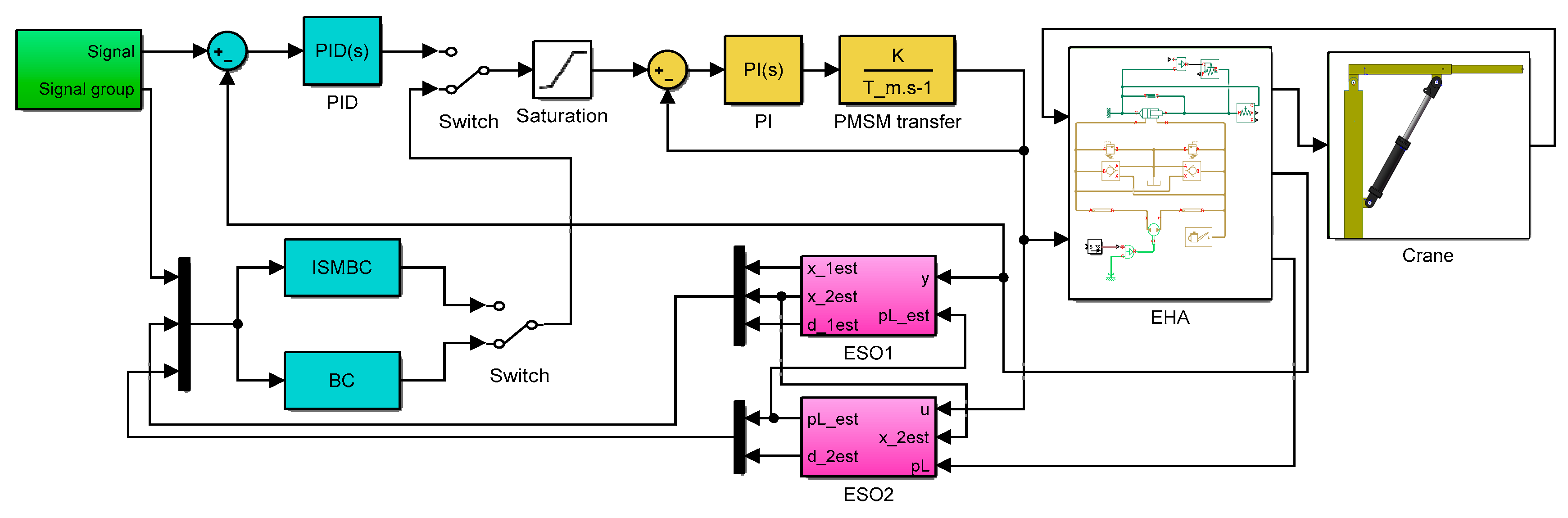
5.1. Simulation Model

To verify the control performance of the proposed controller, a multi-domain model was established in Matlab/Simulink, as shown in Figure 4. The simulation model considers the dynamic response of the motor, the uncertain factors in the hydraulic model including matched disturbance and unmatched disturbance. The parameters of the EHA are shown in

Table 1. Parameters of the EHA.

Parameter (unit)	Symbol	Value	Parameter (unit)	Symbol	Value
mass of boom (kg)	m	30	pump displacement (m3/r)	Dp	13..3 × 10−6
load mass (kg)	ml	0–300	big chamber area (m2)	A1	12.6 × 10−4
gravitational acceleration (m/s2)	g	9.81	small chamber area (m2)	A2	6.4 × 10−4
motor gain (rad/(sA))	K	8.95	total volume (m3)	Vt	4.4 × 10−4
motor time constant (s)	τ	7 × 104	cylinder stroke (m)	s	0.35
effective bulk modulus (Pa)	βe	1.4 × 109	pump leakage coefficient ((m/s)/Pa)	ci	2.93 × 109
critical speed (m/s)	vth	10−4	coulomb friction (N)	FC	50
breakaway friction (N)	Fbrk	100	viscous friction coefficient	f	2000
speed coefficient	cv	10

. To prove the superiority of the designed ISMBC controller, the following three control methods were used for comparison.

(1) Integral sliding mode backstepping control (ISMBC): this is the proposed control scheme in this paper, and the design is described in Section 4. The controller parameters were tuned by hand, k₁ = 4500; k₂ = 100; k₃ = 3; k₀ = 30; w_o = 1000; w_c = 5000; $\mathsf{\rho }=0.5$.

(2) Backstepping control (BC): the control scheme is the same as the ISMBC controller but without integral sliding mode term. To verify the effectiveness of the integral sliding mode control method in the paper, let c₀=0 and $\mathsf{\rho }=0$. Other parameters are the same as those in the ISMBC controller.

(3) Proportional–integral–derivative control (PID): this is a classic control algorithm, which is widely used in industrial fields. This controller realizes the trajectory tracking by tuning the three parameters, including proportional gain k_p, integral gain k_i and derivative gain k_d. Properly increasing these gain parameters can improve the control accuracy, but the excessive gain would also cause oscillation and reduce system stability. Finally, through trial and error, parameters were set as: k_p = 28500; k_i = 1000; k_d = 0.

5.2. Results Analysis

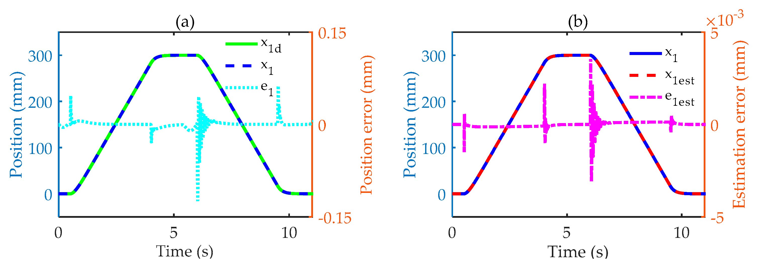
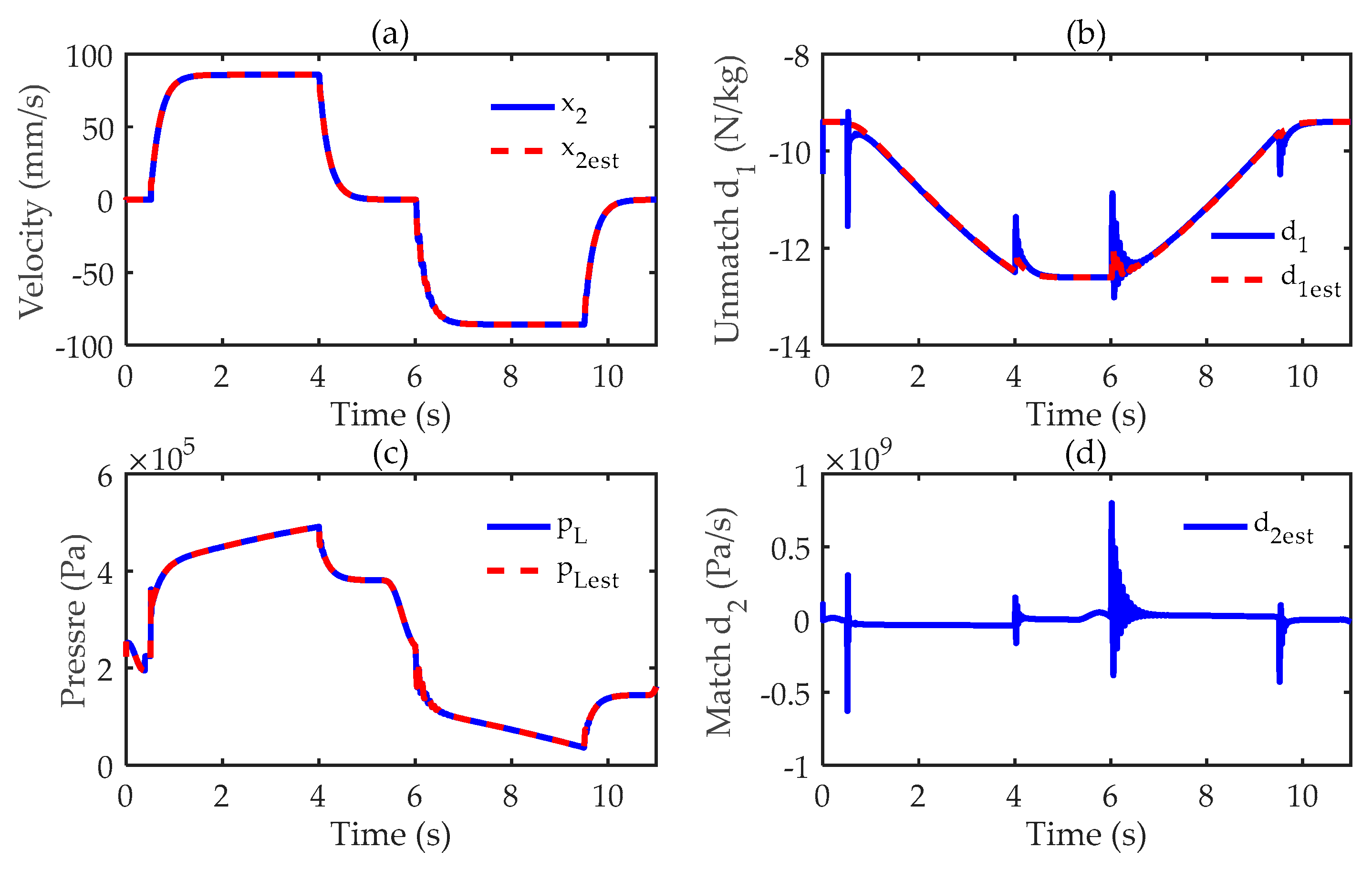
5.2.1. Observer Verification

In view of the fact that the micro-crane mainly performs ascent and descent motions, the controller tracking trajectory was designed as a smooth curve with a max displacement of 0.3 m, starting to rise at t = 0.5 s, and starting to fall at t = 6 s. The desired position of the EHA is shown as the curve x_1d in Figure 5a.

Under the ISMBC controller, the actual output position of the EHA almost overlapped with the reference position signal. The maximum error occurred when the crane just started to descend; the value was 0.124 mm; the EHA mean error was only 3.93 × 10⁻³ mm. It can be seen that the ISMBC controller can achieve high accuracy position control. On the other hand, the position estimation and position estimation error of the ESO1 are shown in Figure 5b. The maximum position estimation error was only 3.52 × 10⁻³ mm. The estimation error was small enough that the observed position can be regarded as the actual output position of the EHA. The estimated values of other state are shown in Figure 6. The observation results show that the designed dual-ESOs can provide accurate feedback values for ISMBC controller and BC controller.

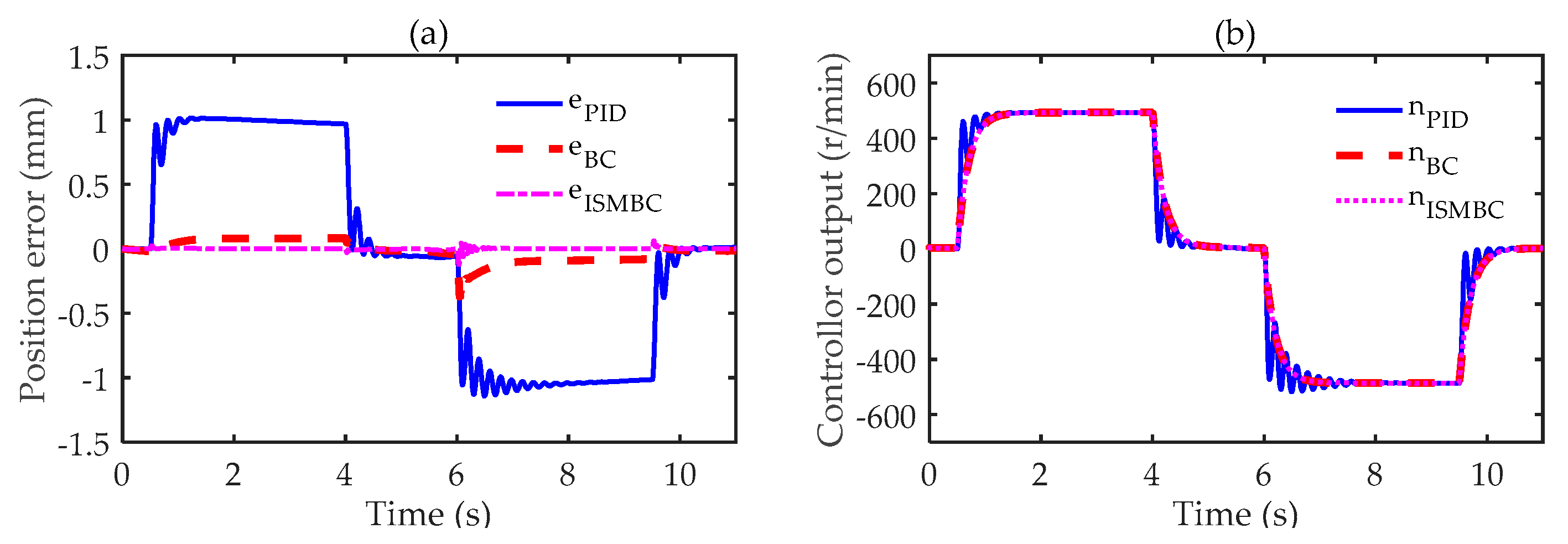
5.2.2. Control Performance without Load

Without load, the three controllers were used for the closed-loop position control of the EHA. The position error and control output of the three controllers are shown in Figure 7a,b, respectively. From Figure 7a, it can be seen that ISMBC possessed the highest control accuracy, and the position tracking error was almost approaching to zero; BC control accuracy was second to ISMBC, which shows that the integral sliding mode surface has the effect of reducing the tracking error. Meanwhile, if PID control is used to achieve higher control accuracy, the proportional gain must be increased, which would cause more severe oscillations to the system. In Figure 7b, the control output curves of the three controllers also prove this point. When the motor speed changes rapidly, the PID control output will oscillate violently, which brings unstable factors to the system. The control output of ISMBC controller and BC controller is smoother.

To intuitively express the control accuracy and stability of each controller, five evaluation indexes were defined to evaluate the performance of the control. Those indexes include maximum tracking error $M_{\mathrm{e}}$, average tracking error ${\mu }_{\mathrm{e}}$, standard deviation of the tracking error ${\sigma }_{\mathrm{e}}$ average controller output ${\mu }_{\mathrm{u}}$ and standard deviation of the controller output ${\sigma }_{\mathrm{u}}$. Without load, the evaluation indexes of the three controllers are listed in

Table 2. Comparison of evaluation indexes of the three controllers without load.

Controller	Me [mm]	μe [mm]	σe [mm]	μu [mm]	σu [mm]
PID	1.14	7.17 × 10−2	0.629	43.28	294.9
ISMBC	0.124	3.93 × 10−3	1.92 × 10−2	1.69	286.9
BC	0.374	3.11 × 10−2	9.10 × 10−2	3.787	272.8

. It can be seen that, except for ${\sigma }_{\mathrm{u}}$, the ISMBC controller had the lowest indexes, so its control performance was the best, followed by BC controller, and the PID control performance was the worst.

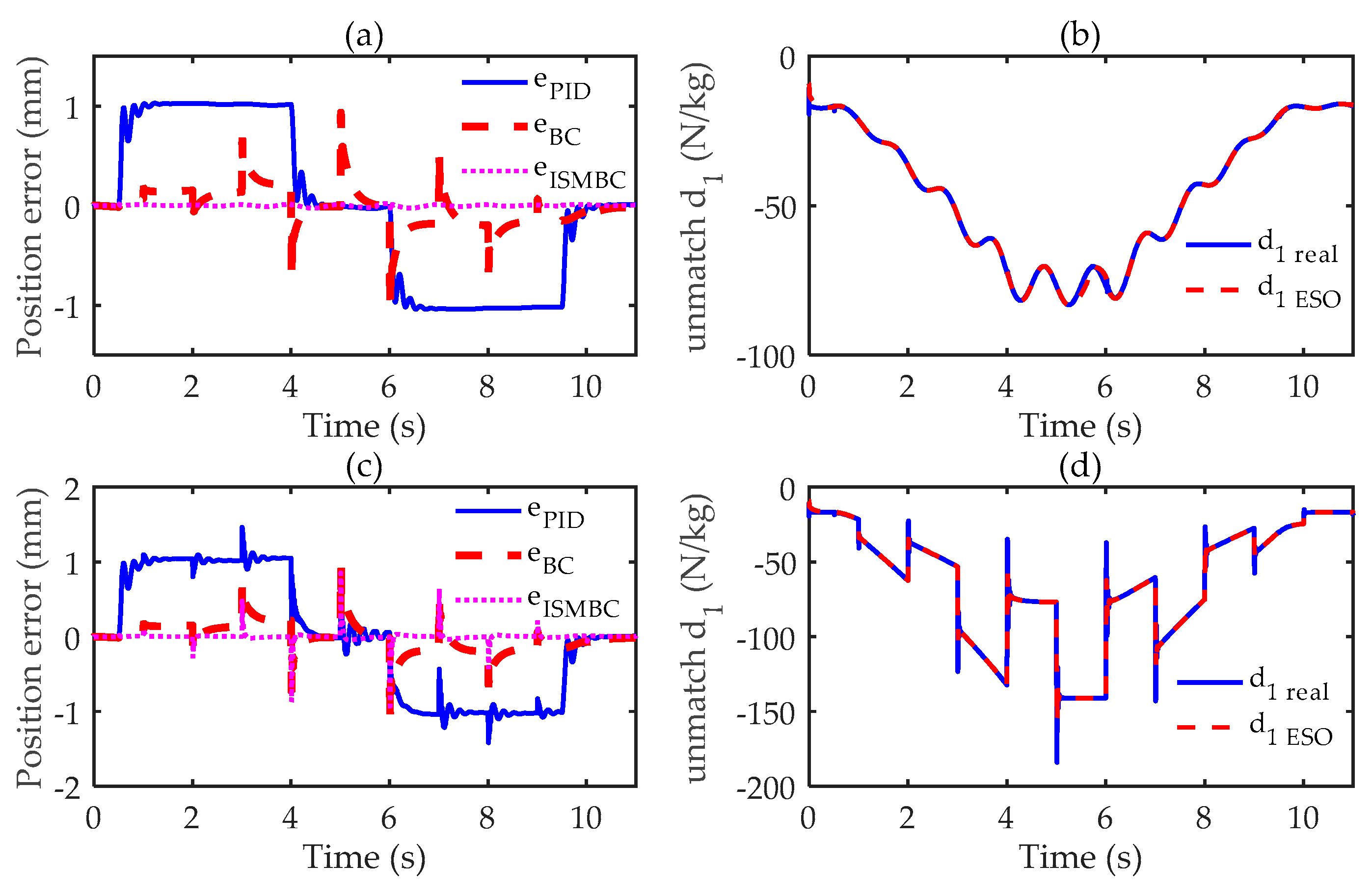
5.2.3. Control Performance with Varing Loads

Figure 8a–c show the different control errors of PID, ISMBC and BC with loads of 100, 200 and 300 kg, respectively. From Section 2.3.2., the main component of the unmatched disturbance is external disturbance, and load is the main source of external disturbance. The ESO1 can accurately estimate the unmatched disturbance with varying loads, to realize the compensation for the unmatched disturbance. The estimated values of unmatched disturbances with varying loads are shown in Figure 8d. Based on the simulation results, the three evaluation indexes $M_{\mathrm{e}}$, ${\mu }_{\mathrm{e}}$ and ${\sigma }_{\mathrm{e}}$ were obtained and listed in

Table 3. Comparison of the evaluation indexes of the three controllers with varying loads.

Controller	Load Mass [mm]	Me [mm]	μe [mm]	σe [mm]
PID	100 kg	1.06	0.112	0.619
	200 kg	1.05	0.103	0.654
	300 kg	1.041	0.121	0.652
BC	100 kg	0.158	0.023	0.079
	200 kg	0.192	0.012	0.099
	300 kg	0.236	0.007	0.115
ISMBC	100 kg	0.073	0.003	0.013
	200 kg	0.061	0.003	0.012
	300 kg	0.052	0.001	0.011

.

From Table 3, it can be found that as the load increased, the indexes gradually decreased with the ISMBC controller. However, with the BC controller, only index ${\mu }_{\mathrm{e}}$ showed a downward trend, and other indexes showed an upward trend. Thus, the results indicate that the integral sliding mode surface can enhance the robustness. In the meantime, only index $M_{\mathrm{e}}$ of the PID controller showed a downward trend, while other indexes showed an upward trend. It shows that within a certain range, larger load force can improve the control performance for the EHA.

5.2.4. Control Performance with Varying Disturbances

The swinging, the sudden increase and decrease in the load mass during motion, would also cause external disturbance. In order to simulate the swinging, a sine force$F_{\sin }=300\sin \left(2\mathsf{\pi }\mathrm{t}\right)$was applied. On this basis, a pulse signal with an amplitude of 3000 N and a period of 2 s was added to simulate the sudden increase and decrease in the load. The simulation results are shown in Figure 9.

From Figure 9a,c, it can be seen that the ISMBC controller was the least affected, followed by the PID controller, and the BC controller was most affected by these external disturbances. This further proves that the integral sliding mode control has stronger anti-disturbance ability.

In summary, compared with the PID controller, the backstepping design can obtain higher control accuracy. In the first step of the backstepping design, the integral sliding mode surface is introduced into the position error term, which not only further improves the control accuracy but also boots the robustness.

6. Conclusions

This paper developed a novel control algorithm ISMBC that introduced integral sliding mode control into backstepping design, based on two extended state observers. The proposed control strategy was applied to solve the problems including nonlinearities, parameter uncertainties and external disturbances in the EHA. Lyapunov analysis showed that the proposed control system has higher stability and better robustness than the traditional backstepping design. A multi-domain model was established in the MATLAB/Simulink, including electric motor, hydraulic system, mechanism of a micro-crane and the proposed ISMBC controller. The following conclusions were obtained by simulation and analysis.

(1) Without load, the ISMBC controller showed the best control accuracy and fastest response. Compared with PID, the control accuracy can be increased by 89% and compared with backstepping control by 67%.

(2) With the loads of 100, 200 and 300 kg, the simulation results show that all control evaluation indexes of the ISMBC controller had a downward trend when load increased. With PID control, only the control accuracy index decreased slightly, and the other indexes showed an overall upward trend. However, all indexes of the BC controller increased.

(3) With load, sinusoidal force disturbance plus step force disturbance signals were applied to the system. The simulation results reveal that the ISMBC had the smallest position error and needed the least time to return to a stable state; the BC control had the largest error, but the oscillation during the recovery process was smaller than PID control.

The results of this study indicate that, compared with the PID controller, the BC controller can greatly improve the control accuracy of the system, but the system stability and robustness degrade. Hence, the ISMBC was proposed, by introducing the integral sliding mode control into the backstepping design. The simulation results show that the proposed ISMBC can not only further improve the control accuracy but also enhance system stability and robustness.

Although the ISMBC control algorithm can improve the control performance of the EHA, it has only been verified by simulation, without being verified by experiment. In the next stage of work, the test platform will be established for further proof and application. On the other hand, the proposed controller relies on accurate system parameters. In the following research, we will use adaptive law to estimate system parameters and to realize adaptive control.

References

1. LI, Z.; Shang, Y.; Jiao, Z.; Lin, Y.; Wu, S.; LI, X. Analysis of the dynamic performance of an electro-hydrostatic actuator and improvement methods. Chin. J. Aeronaut. 2018, 31, 2312–2320. [Google Scholar] [CrossRef]
2. Kuboth, S.; Heberle, F.; Weith, T.; Welzl, M.; König-Haagen, A.; Brüggemann, D. Experimental short-term investigation of model predictive heat pump control in residential buildings. Energy Build. 2019, 204, 109444. [Google Scholar] [CrossRef]
3. Lin, T.; Lin, Y.; Ren, H.; Chen, H.; Chen, Q.; Li, Z. Development and key technologies of pure electric construction machinery. Renew. Sustain. Energy Rev. 2020, 132, 110080. [Google Scholar] [CrossRef]
4. Li, K.; Lv, Z.; Lu, K.; Yu, P. Thermal-hydraulic Modeling and Simulation of the Hydraulic System based on the Electro-hydrostatic Actuator. Procedia Eng. 2014, 80, 272–281. [Google Scholar] [CrossRef]
5. Quan, Z.; Quan, L.; Zhang, J. Review of energy efficient direct pump controlled cylinder electro-hydraulic technology. Renew. Sustain. Energy Rev. 2014, 35, 336–346. [Google Scholar] [CrossRef]
6. Ge, L.; Quan, L.; Zhang, X.; Zhao, B.; Yang, J. Efficiency improvement and evaluation of electric hydraulic excavator with speed and displacement variable pump. Energy Convers. Manag. 2017, 150, 62–71. [Google Scholar] [CrossRef]
7. Fu, S.; Wang, L.; Lin, T. Control of electric drive powertrain based on variable speed control in construction machinery. Automat. Constr. 2020, 119, 103281. [Google Scholar] [CrossRef]
8. Navatha, A.; Bellad, K.; Hiremath, S.S.; Karunanidhi, S. Dynamic Analysis of Electro Hydrostatic Actuation System. Procedia Technol. 2016, 25, 1289–1296. [Google Scholar] [CrossRef]
9. Ur Rehman, W.; Wang, S.; Wang, X.; Fan, L.; Shah, K.A. Motion synchronization in a dual redundant HA/EHA system by using a hybrid integrated intelligent control design. Chin. J. Aeronaut. 2016, 29, 789–798. [Google Scholar] [CrossRef]
10. Xu, Z.; Liu, Y.; Hua, L.; Zhao, X.; Wang, X. Energy improvement of fineblanking press by valve-pump combined controlled hydraulic system with multiple accumulators. J. Clean. Prod. 2020, 257, 120505. [Google Scholar] [CrossRef]
11. Kumar, M. A survey on electro hydrostatic actuator: Architecture and way ahead. Mater. Today Proc. 2020. [Google Scholar] [CrossRef]
12. Altare, G.; Vacca, A. A Design Solution for Efficient and Compact Electro-hydraulic Actuators. Procedia Eng. 2015, 106, 8–16. [Google Scholar] [CrossRef]
13. Mu, T.; Zhang, R.; Xu, H.; Zheng, Y.; Fei, Z.; Li, J. Study on improvement of hydraulic performance and internal flow pattern of the axial flow pump by groove flow control technology. Renew. Energy 2020, 160, 756–769. [Google Scholar] [CrossRef]
14. Lyu, L.; Chen, Z.; Yao, B. Development of parallel-connected pump—Valve-coordinated control unit with improved performance and efficiency. Mechatronics 2020, 70, 102419. [Google Scholar] [CrossRef]
15. Agostini, T.; De Negri, V.; Minav, T.; Pietola, M. Effect of Energy Recovery on Efficiency in Electro-Hydrostatic Closed System for Differential Actuator. Actuators 2020, 9, 12. [Google Scholar] [CrossRef]
16. Gao, B.; Li, X.; Zeng, X.; Chen, H. Nonlinear control of direct-drive pump-controlled clutch actuator in consideration of pump efficiency map. Control. Eng. Pract. 2019, 91, 104110. [Google Scholar] [CrossRef]
17. Ma, X.; Gao, D.; Liang, D. Improved Control Strategy of Variable Speed Pumps in Complex Chilled Water Systems Involving Plate Heat Exchangers. Procedia Eng. 2017, 205, 2800–2806. [Google Scholar] [CrossRef]
18. Sakaino, S.; Tsuji, T. Resonance Suppression of Electro-hydrostatic Actuator by Full State Feedback Controller Using Load-side Information and Relative Velocity. IFAC-PapersOnLine 2017, 50, 12065–12070. [Google Scholar] [CrossRef]
19. Sahu, G.N.; Singh, S.; Singh, A.; Law, M. Static and Dynamic Characterization and Control of a High-Performance Electro-Hydraulic Actuator. Actuators 2020, 9, 46. [Google Scholar] [CrossRef]
20. Ohrem, S.J.; Holden, C. Modeling and Nonlinear Model Predictive Control of a Subsea Pump Station ⁎ ⁎This work was carried out as a part of SUBPRO, a Research-based Innovation Centre within Subsea Production and Processing. The authors gratefully acknowledge the financial support from SUBPRO, which is financed by the Research Council of Norway, major industry partners, and NTNU. IFAC-PapersOnLine 2017, 50, 121–126. [Google Scholar]
21. Wei, S.G.; Zhao, S.D.; Zheng, J.M.; Zhang, Y. Self-tuning dead-zone compensation fuzzy logic controller for a switched-reluctance-motor direct-drive hydraulic press. Proc. Inst. Mech. Eng. Part I J. Syst. Control Eng. 2009, 223, 647–656. [Google Scholar] [CrossRef]
22. Yan, L.; Qiao, H.; Jiao, Z.; Duan, Z.; Wang, T.; Chen, R. Linear motor tracking control based on adaptive robust control and extended state observer. In Proceedings of the 2017 IEEE International Conference on Cybernetics and Intelligent Systems (CIS) and IEEE Conference on Robotics, Automation and Mechatronics (RAM), Ningbo, China, 19–21 November 2017; pp. 704–709. [Google Scholar]
23. Cai, Y.; Ren, G.; Song, J.; Sepehri, N. High precision position control of electro-hydrostatic actuators in the presence of parametric uncertainties and uncertain nonlinearities. Mechatronics 2020, 68, 102363. [Google Scholar] [CrossRef]
24. Lin, Y.; Shi, Y.; Burton, R. Modeling and Robust Discrete-Time Sliding-Mode Control Design for a Fluid Power Electrohydraulic Actuator (EHA) System. IEEE/ASME Trans. Mechatron. 2013, 18, 1–10. [Google Scholar] [CrossRef]
25. Fu, M.; Liu, T.; Liu, J.; Gao, S. Neural network-based adaptive fast terminal sliding mode control for a class of SISO uncertain nonlinear systems. In Proceedings of the 2016 IEEE International Conference on Mechatronics and Automation, Harbin, China, 7–10 August 2016; pp. 1456–1460. [Google Scholar]
26. Alemu, A.E.; Fu, Y. In Sliding mode control of electro-hydrostatic actuator based on extended state observer. In Proceedings of the 2017 29th Chinese Control and Decision Conference (CCDC), Chongqing, China, 28–30 May2017; pp. 758–763. [Google Scholar]
27. Sun, C.; Fang, J.; Wei, J.; Hu, B. Nonlinear Motion Control of a Hydraulic Press Based on an Extended Disturbance Observer. IEEE Access 2018, 6, 18502–18510. [Google Scholar] [CrossRef]
28. WANG, Y.; GUO, S.; DONG, H. Modeling and control of a novel electro-hydrostatic actuator with adaptive pump displacement. Chin. J. Aeronaut. 2020, 33, 365–371. [Google Scholar] [CrossRef]
29. Yang, G.; Yao, J. High-precision motion servo control of double-rod electro-hydraulic actuators with exact tracking performance. ISA Trans. 2020, 103, 266–279. [Google Scholar] [CrossRef]
30. Shen, Y.; Wang, X.; Wang, S.; Mattila, J. An Adaptive Control Method for Electro-hydrostatic Actuator Based on Virtual Decomposition Control. In Proceedings of the 2020 Asia-Pacific International Symposium on Advanced Reliability and Maintenance Modeling (APARM), Vancouver, BC, Canada, 20–23 August 2020; pp. 1–6. [Google Scholar]
31. Yang, G.; Yao, J. Output feedback control of electro-hydraulic servo actuators with matched and mismatched disturbances rejection. J. Frankl. Inst. 2019, 356, 9152–9179. [Google Scholar] [CrossRef]
32. Ren, G.; Costa, G.K.; Sepehri, N. Position control of an electro-hydrostatic asymmetric actuator operating in all quadrants. Mechatronics 2020, 67, 102344. [Google Scholar] [CrossRef]
33. Jing, C.; Xu, H.; Jiang, J. Dynamic surface disturbance rejection control for electro-hydraulic load simulator. Mech. Syst. Signal Process. 2019, 134, 106293. [Google Scholar] [CrossRef]
Figure 1. Structure diagram of the micro-crane.
Proceedings 64 00013 g001
Figure 2. Schematic diagram of an asymmetric electro-hydrostatic actuator (EHA).
Proceedings 64 00013 g002
Figure 3. Schematic diagram of two operating conditions of EHA: (a) the EHA resistive extension; (b) the EHA assistive retraction.
Proceedings 64 00013 g003
Figure 4. Schematic diagram of multi-domain model.
Proceedings 64 00013 g004
Figure 5. Tracking curve and estimation curve of hydraulic cylinder under integral sliding mode backstepping control (ISMBC): (a) position tracking and position error; (b) position estimation and position estimation error.
Proceedings 64 00013 g005
Figure 6. States and disturbances estimation of extended state observers (ESOs) under ISMBC controller: (a) velocity estimation; (b) unmatched disturbance estimation; (c) load pressure estimation; (d) matched disturbance estimation.
Proceedings 64 00013 g006
Figure 7. The comparison of control performance of the three controllers without load: (a) position tracking error; (b) controller output.
Proceedings 64 00013 g007
Figure 8. Position tracking error change of three controllers and external disturbance observation with varying loads: (a) position tracking errors of PID; (b) position tracking errors of BC; (c) position tracking errors of ISMBC; (d) estimation of external disturbances with varying loads.
Proceedings 64 00013 g008
Figure 9. Simulation results of the three controllers with varying disturbances: (a) control errors with sine disturbance; (b) unmatching disturbance observed value with sine disturbance; (c) control errors with sine disturbance plus pulse disturbance; (d) unmatching disturbance observed value with sine disturbance plus pulse disturbance.
Proceedings 64 00013 g009