Proceeding Paper

Machining Quality Prediction Using Acoustic Sensors and Machine Learning †

1
Haute Ecole Arc Ingénierie, University of Applied Sciences and Arts Western Switzerland (HES-SO), CH-2610 St. Imier, Switzerland
2
HEIG-VD, University of Applied Sciences and Arts Western Switzerland (HES-SO), CH-1401 Yverdon-les-Bains, Switzerland
*
Author to whom correspondence should be addressed.
Presented at the 14th International Conference on Interdisciplinarity in Engineering—INTER-ENG 2020, Târgu Mureș, Romania, 8–9 October 2020.
Proceedings 2020, 63(1), 31; https://doi.org/10.3390/proceedings2020063031
Published: 17 December 2020

Abstract

:
The online automatic estimation of the quality of products manufactured in any machining process without any manual intervention represents an important step toward a more efficient, smarter manufacturing industry. Machine learning and Convolutional Neural Networks (CNN), in particular, were used in this study for the monitoring and prediction of the machining quality conditions in a high-speed milling of stainless steel (AISI 303) using a 3 mm tungsten carbide. The quality was predicted using the Acoustic Emission (AE) signals captured during the cutting operations. The spectrograms created from the AE signals were provided to the CNN for a 3-class quality level. A promising average f1-score of 94% was achieved.

1. Introduction

In this paper, we investigate the automatic detection of quality degradation during a milling machining process by analyzing the acoustic signature of the machining process using neural networks. Such a degradation is often due to the inevitable tool wear resulting from any metal cutting process. Typical tool wear is characterized by three stages: break-in, steady state, and failure [1]. Break-in indicates the rapid process that transforms and wears the tool when it is first used. Afterwards, and for most of the tool’s lifespan, the tool’s wear increases gradually; here, the tool is in a steady-state condition. Finally, failure represents a rapidly deterioration phase at the end of the tool’s life.
Reliable continuous quality monitoring would allow real-time decision-making to adjust the machining process when the process is about to produce an undesired surface quality in the workpiece (e.g., replacing a machining tool, changing cutting parameters, etc.). In this paper, we investigate Acoustic Emission (AE) sensors for the indirect monitoring of machining quality. AE sensors are used to detect the high-frequency waves that are provoked by the metal-cutting process. AEs typically include a frequency range from 100 to 1 MHz [2]. The analysis of the AE allows the characterization of the process without a direct observation of the workpiece, thereby possibly avoiding the wasting of material, tools breaking, and unplanned production stops (unplanned equipment downtime).

Theoretical Background

The usage of sensors for the monitoring of cutting processes has been studied for several years. In this context, previous research has demonstrated that the acoustic signals analyzed during an industrial process can contain features which could be used to automatically estimate the quality of the process itself [3,4]. If this is compared to traditional manual interventions, AE signals can be acquired without interfering with the cutting process, and the sensed frequency range is much higher compared to other sensors such as accelerometers. The previous works used AE (often in combination with other sensors) for the prediction and monitoring of the state of the surface, gear grinding [5,6,7], turning [8,9] and the analysis of scuffing [10]. The surface quality and the tool wear are the variables that are typically monitored. AE sensors have also been studied in other manufacturing processes, such as additive manufacturing [3].
Our study is focused on milling machining for high-precision industry (the watch and automotive industries). Specifically, milling is a machining process that aims to remove material using rotating cutters. For the analysis of different manufacturing operations, AE sensors have been often used in combination (or compared with) other sensors, such simpler microphones [11], force and power measurements [12], vibration acceleration sensing [13,14], and infrared cameras [15] (for a general survey of data-driven monitoring in the manufacturing process, a reader can refer to the survey of Xu et al. [16]).
The usage of Acoustic Emission sensors for the monitoring of machining processes has been investigated for several years, but the recent availability of data-driven learning solutions based on Machine Learning opens the path to the analysis of larger amounts of data from sensors that have higher dynamics. Machine Learning approaches have shown potential for making better decisions to monitor and, finally, to automate the machining process. Different algorithms are used in the literature, such as Support Vector Machines [11,17], Hidden Markov Models [18], decision trees [14], and (deep) neural networks (such as Convolutional Neural Networks, Long Short-Term Memory networks, etc.) [9].
In this study, we want to investigate the machine learning performances that can be achieved by reducing—at the bare minimum—the pre-processing and feature extraction steps, using only the information from AE sensors. In a similar work, Krishnan et al. [18] extracted the milling process signature and used Hidden Markov modelling for the prediction of the tool conditions. Their study showed a promising correlation between the AE signal features and the tool conditions. In their study, the features were manually extracted. We focus our study on the usage of Convolutional Neural Networks (CNN) [19] for the automatic extraction of the relevant features.
The rest of the paper is organized as follows: sect:sec2-proceedings-63-00031 will describe the materials and the methodology used to acquire the dataset, including the data labeling approach. sect:sec3-proceedings-63-00031 will present the realized data processing and machine learning architecture. Finally, sect:sec4-proceedings-63-00031 will discuss the results achieved.

2. Materials, Methods and Data Acquisition

2.1. Materials

A milling machine, called ‘Micro5’ (Figure 1), was used for the cutting process. The Micro5 machine belongs to a novel category of milling machines characterized by their small size and the related improved efficiency.
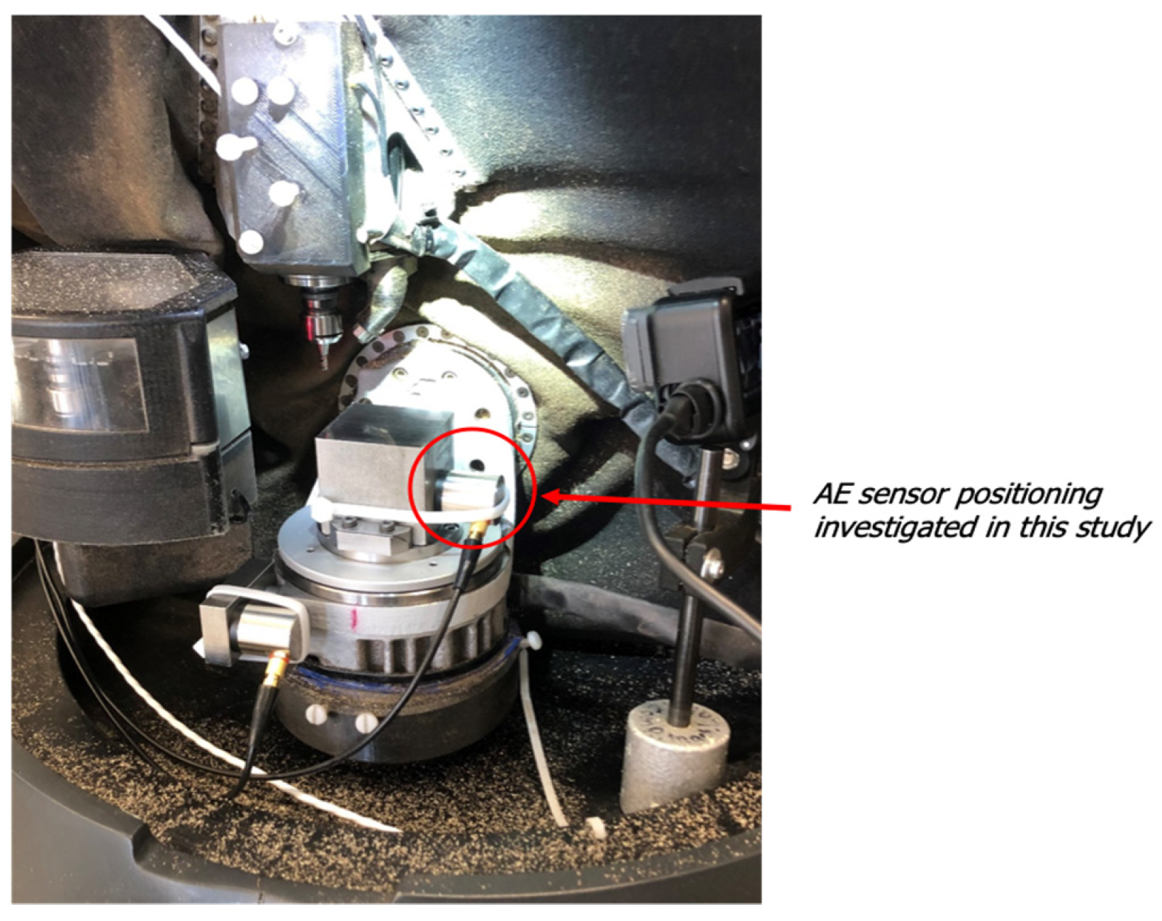
The sensor used for the acquisition was a Vallen VS45-H. This sensor is a piezoelectric AE-sensor with a wide frequency response. This sensor can be used in a frequency range between 40 kHz and 450 kHz. For this project, we limited the maximum sampling rate to 200 kHz. Resulting from our use of the Nyquist–Shannon sampling theorem, we limited our study to frequencies between 40 kHz and 100 kHz. The AE sensor was placed in direct contact with the raw material, as displayed in the figure below (Figure 2).

2.2. Methodology: Data Acquisition, Labeling and Classification

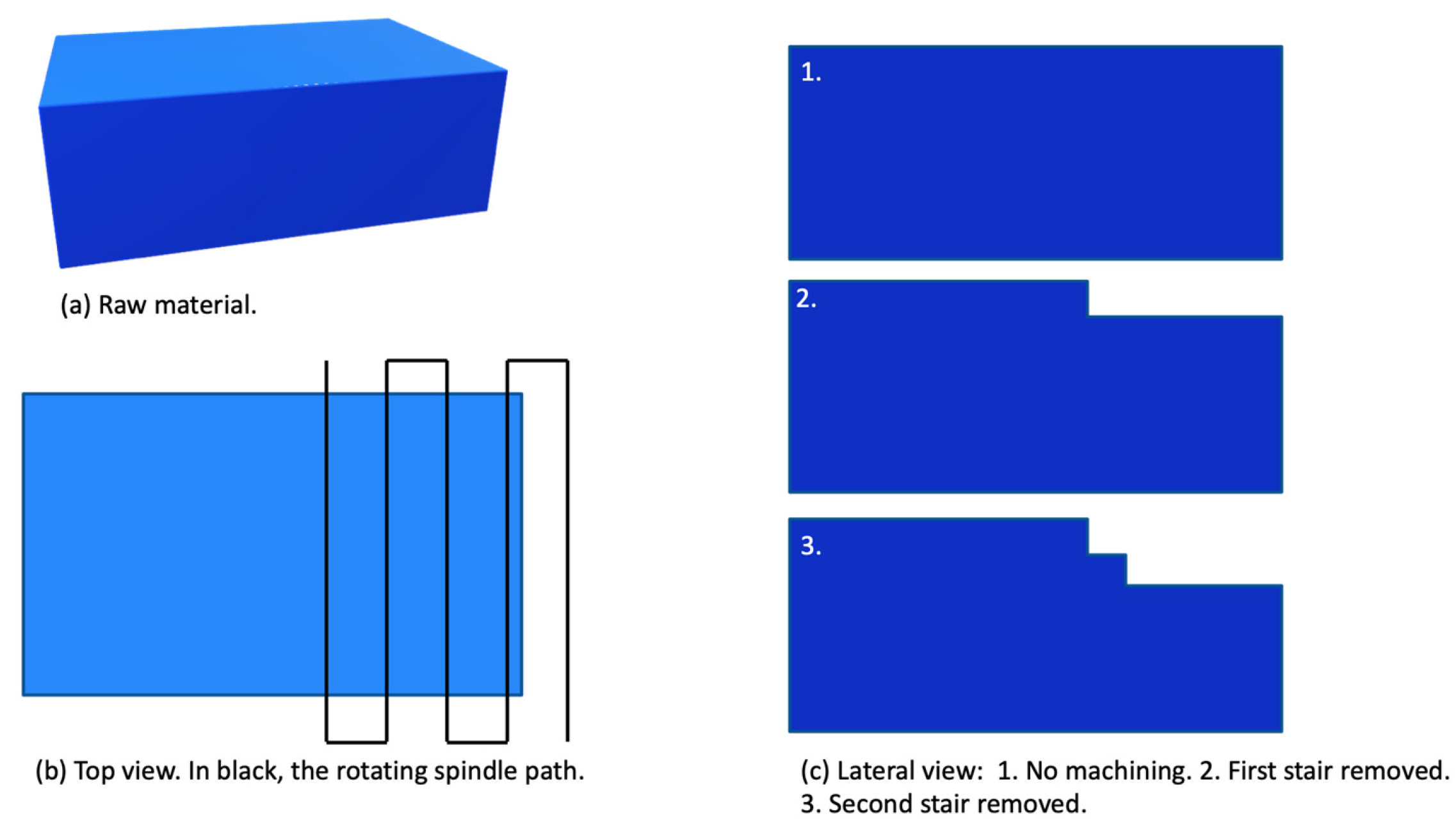
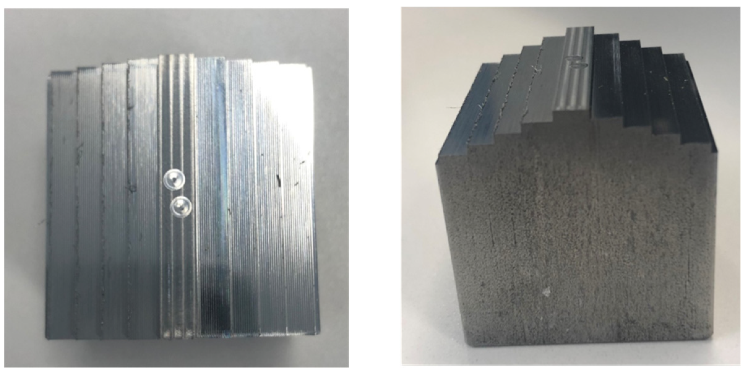
For the experimentation, we used a milling machine working with stainless steel (AISI 303) and no lubrication. A tungsten carbide tool with a 3 mm diameter was used for the machining. The cutting process consisted in simple linear passes at different heights (creating a stair-shaped workpiece, as illustrated in Figure 3). Once half of the material was machined, the process was repeated symmetrically. Figure 4 shows the resulting part.
At the beginning of each experience, the tool is new. The machining ends and the tool is replaced if one of the following conditions is verified:
label=0.
the tool breaks;
lbbel=0.
the tool is considered ‘too used’ by an expert human;
lcbel=0.
the workpiece is completely machined (6 stairs).

2.3. Milling Dataset

In order to train the supervised machine learning algorithms, the creation of a labeled dataset is needed. The materials presented in the previous sections were used to realize multiple workpieces; the acquired data represent the dataset used for the study. Table 1 summarizes the conditions and the different experiences realized.
Experiences 1, 2, and 3 did not involve any actual machining. The tool was mounted on the machine, but the material was not processed. In experience 1, the milling machine was turned on and the spindle was not turning. In experiences 2 and 3, the spindle was turning at 29,000 and 35,000 revolutions per minute respectively, but the cutting tool was not touching the material. This allows the characterization of the signal ‘noise’ generated by the machine, rather than by the contact between the tool and the material. Actual machining with the tool cutting the material was recorded for experiences 4, 5, and 6. The last column presents the encoding of the observed labels: 0 stands for ‘good quality’, 1 for ‘intermediate quality’, and 2 for ‘bad quality’.
A simple observation of the dataset allows us to notice the impact of the spindle’s rotation speed on the machining quality degradation. In the given configuration, a lower RPM allowed the process to maintain a better machining quality for a longer time. A higher RPM quickly degraded the machining quality (due to faster tool wear).

2.4. Labeling Approach

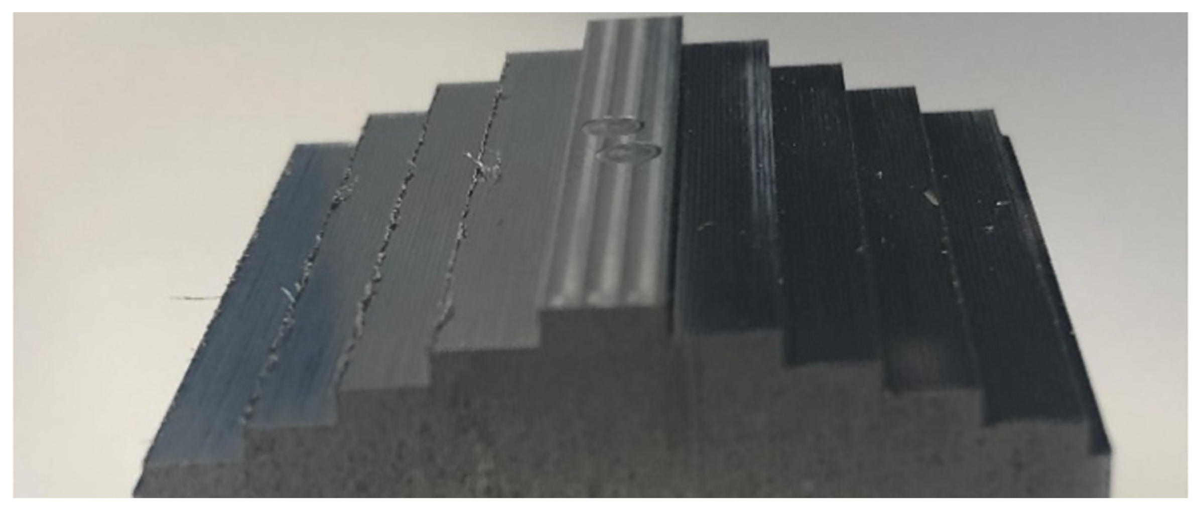
In order to label the dataset, the quality of the machining was computed with the help of the observed surface roughness. As mentioned in the previous paragraph, in this project, we considered three different quality labels (good, intermediate and poor quality). It is important to highlight that the process quality was observed and measured only at the end of the machining of the resulting parts. This implies that the quality of the machining and the related label (used as the ground truth and labels in the analyses) can be assessed only for the particular steps of the process on the surface of the remaining material (see Figure 5).
As shown in Table 1, the acquired database is relatively small. The labeling approach generated only 15 labels, one per stair. In order to augment the labels in the dataset and to make it suitable for the Machine Learning approach, we decided to extend the labels to each pass through the material (multiple passes are required to machine one stair). The stair labels were extended to each pass of the spindle on the material through a linear interpolation. The passes outside the material, when the tool is moving but it is not touching the material, were removed. This allowed us to increase the number of labels from 15 to 544.

2.5. Feature Extraction

Instead of using the raw acoustic data directly as our model input, we converted the value of these sensors into the frequency domain. Several time/frequency transformation approaches were evaluated (wavelet transformation, constant Q-transformation, etc.); in this paper, we present the results achieved with a spectrogram based on the Fast Fourier Transform (FFT) approach (1024 FFTs with a window overlap of 512).
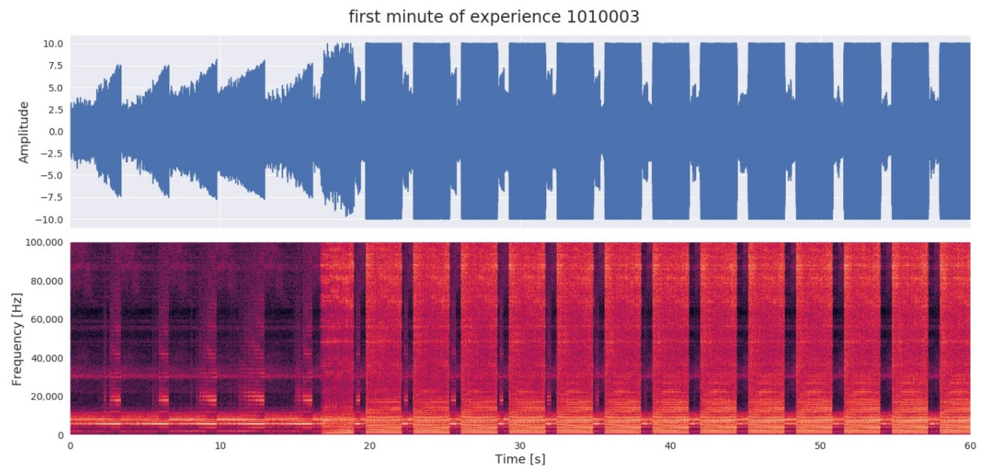
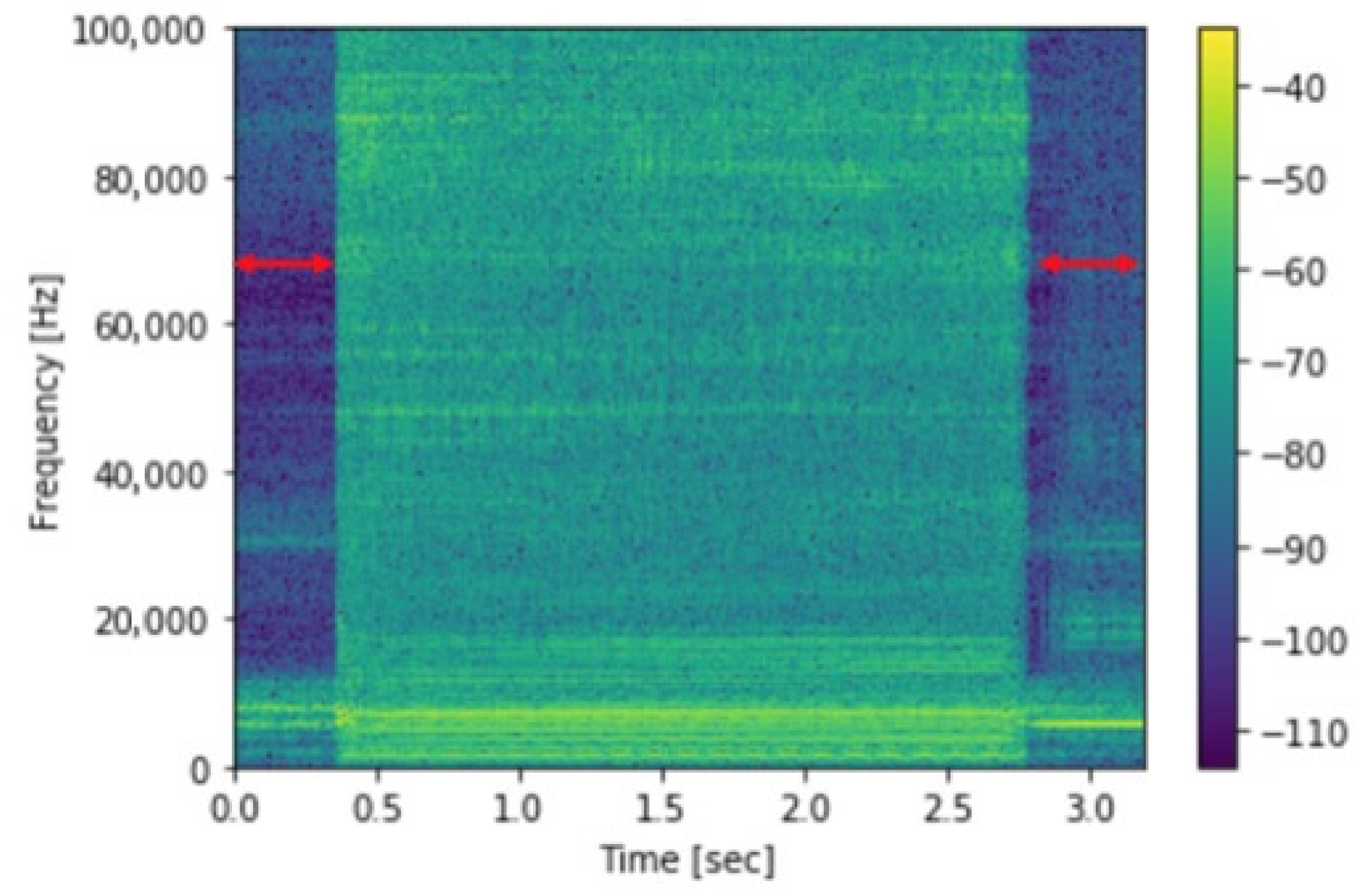
Figure 6 shows an example of 1 minute of the acoustic signal (top part of the figure) and the resulting spectrogram (bottom part). On the first passes on the left, the tool is not touching the material. The periodic pattern shows the different passes in the material. Figure 7 zooms in on the spectrogram generated by one pass.
In the middle of the spectrogram, we can observe a clearer area. This section represents when the tooling machine is actively machining the material and more frequencies are being captured. The darker areas represent the machining portions when there is no contact between the tool and the workpiece. An interesting approach to exploit this data could be to subtract the machine noise signature from the machining noise; however, this approach has not been explored in this paper.
Finally, before providing the spectrograms to the neural network, the inputs were resized to a constant size of 126 × 126 points.

2.6. Classification

The spectrograms generated by the feature extraction preprocessing can be used as image-like inputs for the classification task. Image classification is a well-documented problem; today, one of the most frequently-used approaches for such tasks is the Convolutional Neural Network (CNN). This deep learning model is trained to automatically recognize patterns in images, and to associate such patterns with the appropriate label. The architecture of our CNN is as follows: two convolutional layers, the purpose of which is to extract features from the inputted images, followed by two dense layers for the classification itself. For the convolutions, 32 and 64 filters, 3 × 3, were used respectively for the first and second layers. The max pooling and dropout layers were used to reduce the computational cost of the learning, and to reduce the risk of overfitting (a model with high variance and low bias [20]). The details of the implementations are presented in Appendix A.
In order to assess the training process quality, we decided to adopt a cross-validation approach. Cross-validation is used in applied machine learning to estimate the quality of a machine learning model, and it is particularly relevant for small datasets. The goal is to estimate how the model is expected to perform when it is used to make predictions on data that are not seen during the training of the model. The approach used here is a k-folds cross-validation with k = 5. The idea behind the k-fold validation is to split k times the dataset into training and validation sets. As the name implies, for each fold, the newly created training set will be used to train the model, while the validation set (unseen by the model) will be used to evaluate its classification performance. Then, 138 sur 544 images were used in the test set. Among other parameters (such as network complexity), the number of epochs used to train a dataset affects the bias and variance of a classifier. In particular, the more epochs are used to train the dataset, the higher the risk of overfitting. A common approach to limit overfitting is to observe the behavior of the training and validation loss after each epoch during the whole training process. If the training loss tends to get smaller and smaller while the validation loss increases, then we can clearly see that the model is starting to memorize the training set instead of learning general patterns: it is overfitting. The observation of training and validation loss allows for a deeper understanding of the model’s behaviors; it not only gives insight about whether or not the model is overfitting, but also about when it started to happen. The knowledge of when the model starts to overfit allows the use of a technique called early stopping. As the name implies, this will shorten the training process if necessary. The stopping condition is based on the validation loss and how it behaves: if—after converging for a while—it starts going back up, then we know the model is starting to overfit. Categorical cross-entropy was used as the loss function, using Adam as the optimizer.

3. Results

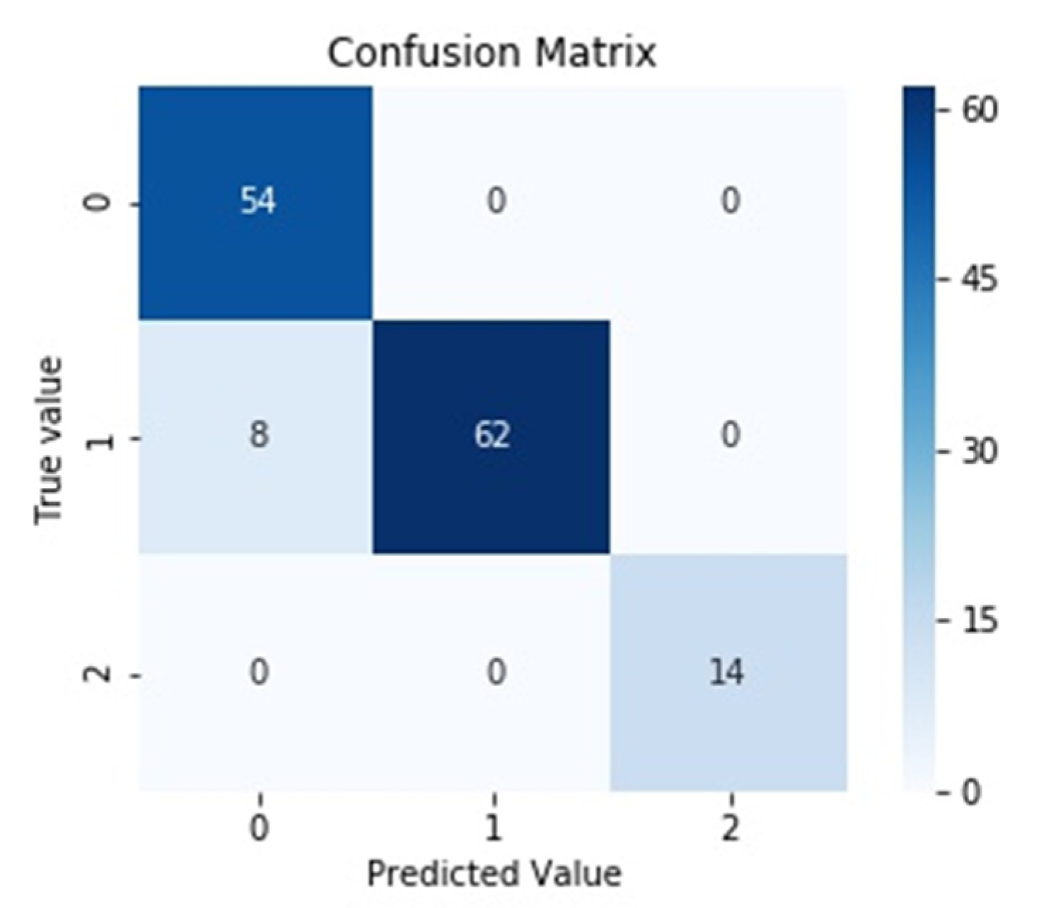
Our classification performances were computed over multiple runs using a confusion matrix (displayed in Figure 8) and an f1-score on a test set that was unseen during the training phase. The f1-score (also called the f-measure) is the harmonic mean of the Precision and Recall [21]. Overall, on these runs, the model achieved an average f1-score of 94% and, as mentioned in the previous section, we reduced the overfitting risk with the help of a 5-fold cross-validation approach, regularization, and dropout layers. Since the dataset is unbalanced (labels 0 and 1 are more represented than label 2), we preferred the f1-score over other metrics, such as accuracy.

4. Discussion

As shown in the confusion matrix (Figure 8), only a few data points were misclassified by the neural network solution. In addition, the misclassified points belong to the middle class 1, indicating an intermediate quality of the machining: the classifier never confuses ‘good’ quality with ‘bad’ quality. All of the misclassified points were classified with the 0 label; this could be due to the unbalanced dataset, but further analysis is needed to assess this point.
Concerning the computational performances, the filtering of the signal directly after the acquisition and the generation the spectrogram can be achieved in pseudo-real time. Considering the typical length of a machining process (from a few seconds to several minutes), the proposed classifier can predict the quality of the machining directly during the process. The AE sensor’s high sampling frequency leads to a rapidly-growing dataset, even for rather short cutting operations. In this study, we collected data during the whole processing. However, most of the data are redundant: for instance, the data at the beginning of a pass are quite similar to the data at the end of the same pass. In order to shorten the computation time, it can be opportune to reduce the time windows used to generate the spectrogram to few milliseconds. Instead of collecting data for a whole pass, just a significant fraction of the data can be collected. These results are extremely promising because they show that it is possible to detect the quality of a machining process without directly observing the realized workpiece. This observation has several practical consequences:
  • Additional machines to assess the quality can be removed from the production line.
  • If the quality estimation can be performed on the fly during the machining, tool breakage and material and time wastage can be avoided.
Nevertheless, the presented results were achieved in a particular set of conditions, and further analyses are needed in order to validate these results in a more general context. The current limitations include:
  • The small dataset.
  • The fact that realized milling process is simple, as it consists of linear passes repeated at different heights. More complex cutting operations can generate noise that could be more difficult to analyze.
  • Only one type of material was used, along with one type of tool and one type of lubrication (no lubrication).
In order to address these limitations, we plan to evaluate the model’s performance on a larger dataset acquired in different machining conditions. The presented 3-class classification problem will be adapted into a multi-objective regression formulation in order to directly predict the surface roughness and dimensional quality (given nominal values to achieve for a specific task). From an applied perspective, the novel approach has the advantage of being easier to adapt to different scenarios. According to the context of utilization, it will be possible to decide for each specific use case what can be considered to be ‘good’ or ‘bad’ machining by fixing the appropriate thresholds. For instance, for a precision workpiece used in the watchmaking industry, minimal variations can have a huge impact on the functioning of a watch, whereas such strict requirements are not required in other domains, and the machining constraints can be relaxed.

Author Contributions

S.C. coordinated the research, conceived the presented approach and extracted the features from the raw signals. J.G. conceived and developed the machine learning solution (CNN); J.D. worked on the results analyses together with H.G., A.S. contributed with the sensor selection, their installation on the machine and a data validation step. R.M. coordinated the mechanical tasks with the Micro5: from the conception to the parts to the actual machining of the parts. All authors have read and agreed to the published version of the manuscript.

Funding

This research was internally funded by the University of Applied Sciences and Arts Western Switzerland (HES-SO) and the CHIST-ERA program (SOON project).

Acknowledgments

These results could not have been achieved without the help of the technical team involved in the instrumentation of the machine; the design and implementation of the machining plan; and the data retrieval, storing and pre-processing. In particular, the authors want to thank Jeshon Assunçao, Damien Heiniger, Jérémy Terrier, Adrien Limat, Nima Pakpoor Gilani, Nicolas Jacquod and Célien Donzé.

Conflicts of Interest

The authors declare no conflict of interest. The funders had no role in the design of the study; in the collection, analyses, or interpretation of data; in the writing of the manuscript, or in the decision to publish the results.

Appendix A

The convolution architecture is detailed with the following summary (generated using Keras API, http://keras.io/ and then adjusted for publication).
Table A1. CNN model summary.
Layer (Type)Output ShapeParam #
Conv2D (relu)(None, 126, 126, 32)320
Conv2D (relu)(None, 124, 124, 64)18496
MaxPooling2D(None, 62, 62, 64)
Dropout(None, 62, 62, 64)
Flatten(None, 246016)
Dense(None, 128)31490176
Dropout(None, 128)
Dense (softmax)(None, 3)387
Total params: 31,509,379
Trainable params: 31,509,379
Non-trainable params: 0

References

  1. Dou, J.; Xu, C.; Jiao, S.; Li, B.; Zhang, J.; Xu, X. An unsupervised online monitoring method for tool wear using a sparse auto-encoder. Int. J. Adv. Manuf. Technol. 2020, 106, 2493–2507. [Google Scholar] [CrossRef]
  2. Dornfeld, D.A.; Lee, Y.; Chang, A. Monitoring of Ultraprecision Machining Processes. Int. J. Adv. Manuf. Technol. 2003, 21, 571–578. [Google Scholar] [CrossRef]
  3. Shevchik, S.A.; Masinelli, G.; Kenel, C.; Leinenbach, C.; Wasmer, K. Deep Learning for In Situ and Real-Time Quality Monitoring in Additive Manufacturing Using Acoustic Emission. IEEE Trans. Ind. Inf. 2019, 15, 5194–5203. [Google Scholar] [CrossRef]
  4. Inasaki, I. Application of acoustic emission sensor for monitoring machining processes. Ultrasonics 1998, 36, 273–281. [Google Scholar] [CrossRef]
  5. Mouli, D.S.B.; Rameshkumar, K. Acoustic Emission-Based Grinding Wheel Condition Monitoring Using Decision Tree Machine Learning Classifiers. In Advances in Materials and Manufacturing Engineering; Li, L., Pratihar, D.K., Chakrabarty, S., Mishra, P.C., Eds.; Lecture Notes in Mechanical Engineering; Springer: Singapore, 2020; pp. 353–359. ISBN 9789811513060. [Google Scholar]
  6. Sachin Krishnan, P.; Rameshkumar, K. Grinding wheel condition prediction with discrete hidden Markov model using acoustic emission signature. Mater. Today Proc.
  7. Arun, A.; Rameshkumar, K.; Unnikrishnan, D.; Sumesh, A. Tool Condition Monitoring of Cylindrical Grinding Process Using Acoustic Emission Sensor. Mater. Today Proc. 2018, 5, 11888–11899. [Google Scholar] [CrossRef]
  8. Li, X. A brief review: Acoustic emission method for tool wear monitoring during turning. Int. J. Mach. Tools Manuf. 2002, 42, 157–165. [Google Scholar] [CrossRef]
  9. Ibarra-Zarate, D.; Alonso-Valerdi, L.M.; Chuya-Sumba, J.; Velarde-Valdez, S.; Siller, H.R. Prediction of Inconel 718 roughness with acoustic emission using convolutional neural network based regression. Int. J. Adv. Manuf. Technol. 2019, 105, 1609–1621. [Google Scholar] [CrossRef]
  10. Saeidi, F.; Shevchik, S.A.; Wasmer, K. Automatic detection of scuffing using acoustic emission. Tribol. Int. 2016, 94, 112–117. [Google Scholar] [CrossRef]
  11. Zhang, K.; Yuan, H.; Nie, P. A method for tool condition monitoring based on sensor fusion. J. Intell. Manuf. 2015, 26, 1011–1026. [Google Scholar] [CrossRef]
  12. Chung, K.T.; Geddam, A. A multi-sensor approach to the monitoring of end milling operations. J. Mater. Process. Technol. 2003, 139, 15–20. [Google Scholar] [CrossRef]
  13. Cao, X.; Chen, B.; Yao, B.; Zhuang, S. An Intelligent Milling Tool Wear Monitoring Methodology Based on Convolutional Neural Network with Derived Wavelet Frames Coefficient. Appl. Sci. 2019, 9, 3912. [Google Scholar] [CrossRef]
  14. Krishnakumar, P.; Rameshkumar, K.; Ramachandran, K.I. Tool Wear Condition Prediction Using Vibration Signals in High Speed Machining (HSM) of Titanium (Ti-6Al-4V) Alloy. Procedia Comput. Sci. 2015, 50, 270–275. [Google Scholar] [CrossRef]
  15. Luiz Lara Oliveira, T.; Zitoune, R.; Ancelotti, A.C., Jr.; Cunha, S.S., Jr. da Smart machining: Monitoring of CFRP milling using AE and IR. Compos. Struct. 2020, 249, 112611. [Google Scholar] [CrossRef]
  16. Xu, K.; Li, Y.; Liu, C.; Liu, X.; Hao, X.; Gao, J.; Maropoulos, P.G. Advanced Data Collection and Analysis in Data-Driven Manufacturing Process. Chin. J. Mech. Eng. 2020, 33, 43. [Google Scholar] [CrossRef]
  17. Krishnakumar, P.; Rameshkumar, K.; Ramachandran, K.I. Machine learning based tool condition classification using acoustic emission and vibration data in high speed milling process using wavelet features. IDT 2018, 12, 265–282. [Google Scholar] [CrossRef]
  18. Sachin Krishnan, P.; Rameshkumar, K.; Krishnakumar, P. Hidden Markov Modelling of High-Speed Milling (HSM) Process Using Acoustic Emission (AE) Signature for Predicting Tool Conditions. In Advances in Materials and Manufacturing Engineering; Li, L., Pratihar, D.K., Chakrabarty, S., Mishra, P.C., Eds.; Lecture Notes in Mechanical Engineering; Springer: Singapore, 2020; pp. 573–580. ISBN 9789811513060. [Google Scholar]
  19. Krizhevsky, A.; Sutskever, I.; Hinton, G.E. ImageNet Classification with Deep Convolutional Neural Networks. In Proceedings of the 25th International Conference on Neural Information Processing Systems-Volume 1; Curran Associates Inc.: Red Hook, NY, USA, 2012; pp. 1097–1105. [Google Scholar]
  20. Hawkins, D.M. The Problem of Overfitting. J. Chem. Inf. Comput. Sci. 2004, 44, 1–12. [Google Scholar] [CrossRef] [PubMed]
  21. Hripcsak, G. Agreement, the F-Measure, and Reliability in Information Retrieval. J. Am. Med Inform. Assoc. 2005, 12, 296–298. [Google Scholar] [CrossRef] [PubMed]
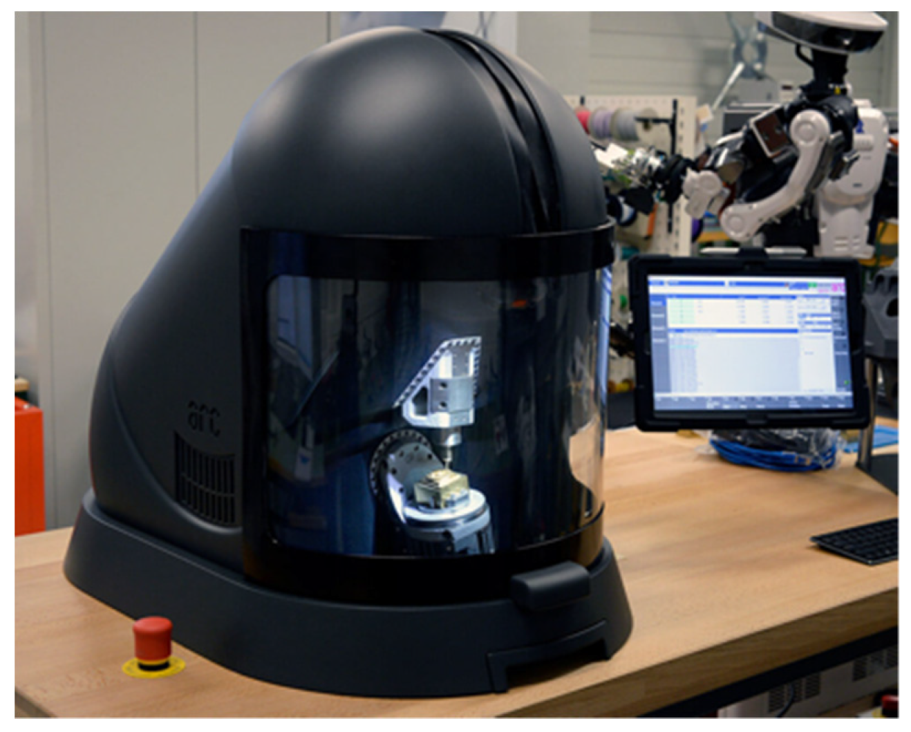
Figure 1. The Micro5, the milling machine used in this study.
Proceedings 63 00031 g001
Figure 2. Acoustic emission sensor positioning. As highlighted by the red circle, the AE sensor is glued to the material that is being machined.
Proceedings 63 00031 g002
Figure 3. A visual representation of the milling operation investigated in this study. (a) The raw material before the machining; (b) in black, from the right to the left, the path of the cutting tool. In the representation, we can observe 5 passes, of which 1 is outside the material, and 4 are in the material–top view. (c) Removal of the first 2 levels of the material-lateral view.
Proceedings 63 00031 g003
Figure 4. Pictures of one of the resulting workpieces.
Proceedings 63 00031 g004
Figure 5. This figure shows the details of a workpiece. The left side was machined with a tool at the end of its lifespan. The presence of multiple chips in the material indicates that the quality of the stair edges has deteriorated.
Proceedings 63 00031 g005
Figure 6. Transformation of the signal from the time domain to the related spectrogram. On the left, we can observe that the first 5 passes are outside the material (no-machining), the sixth touches the material only partially, and the following passes characterize the normal machining behavior.
Proceedings 63 00031 g006
Figure 7. A typical spectrogram of one pass. In the dark blue vertical areas, highlighted by the red arrows, the tool is outside of the machining area. The color, in log scale, represents the intensity of the signal.
Proceedings 63 00031 g007
Figure 8. Classification performance of the model for one run.
Proceedings 63 00031 g008
Table 1. Summary of the different experiences realized. Only the data from experiences 4, 5 and 6 were used to train the evaluating Machine Learning solutions.
Experience IDSpindle Rotation Speed (Revolutions per Minute)Number of Stairs MachinedQuality Label: 0 (Good), 1 (Intermediate), 2 (Bad)
10 RPM-
229k RPM-
335k RPM-
429k RPM0, 0, 0, 1, 1, 1
533k RPM1, 1, 1, 1, 1
635k RPM1, 2, 2
Publisher’s Note: MDPI stays neutral with regard to jurisdictional claims in published maps and institutional affiliations.