Proceeding Paper

Detecting and Correlating Aircraft Noise Events below Ambient Noise Levels Using OpenSky Tracking Data †

Group Waves, Information Technology, Ghent University, B-9000 Ghent, Belgium
Presented at the 8th OpenSky Symposium 2020, Online, 12–13 November 2020.
Proceedings 2020, 59(1), 13; https://doi.org/10.3390/proceedings2020059013
Published: 3 December 2020
(This article belongs to the Proceedings of 8th OpenSky Symposium 2020)

Abstract

:
Noise annoyance due to aircraft operations extends well beyond the 55 Lden noise contours as calculated according to the Environmental Noise Directive (END). Noise mapping beyond these contours will improve the understanding of the perception, annoyance and health impact of aircraft operations. OpenSky data can provide the spatial data to create an aircraft noise exposure map for lower exposure levels. This work presents the first step of region-wide noise exposure methodology based on open source data: detecting low LAmax aircraft events in ambient noise using spectral noise measurements and correlating the detected noise events to the matching flights retrieved from the OpenSky database. In ISO 20906:2009, the specifications of noise monitoring near airports is standardized, using LAeq,1sec values for event detection. This limits the detection potential due to masking by other noise sources in areas with low maximum levels of aircraft noise and in areas with medium maximum levels of high ambient exposure areas. The typical lower detection limit in airport-based monitoring systems ranges from 55 to 60 LAeq,max, depending on the ambient levels. Using a detection algorithm sensitive to third-octave band levels, aircrafts can be detected down to 40 LAmax in ambient noise levels of a similar magnitude. The measurement approach is opportunistic: aircraft events are detected in available environmental noise data series registered for other applications (e.g., road noise, industrial noise, etc.). Most of the measurement locations are not identified as high-exposure areas for aircraft noise. Detection settings can vary to match ambient noise levels to improve the correlation success.

1. Introduction

1.1. Current Practice in Aircraft Noise Mapping and Noise Event Monitoring

The evaluation of noise exposure is organized at EU-level by the European Commission. In the Environmental Noise Directive (END), the lowest threshold to report aircraft noise is set to Lden 55 dBA and Lnight 45 dB [1]. Exposure assessments near airports are well documented and are standardized to fulfil the quality requirements of the Environmental Noise Directive [1]. These exposure models are very accurate and are available in a wide range of commercial and non-commercial software packages. The European Union Aviation Safety Agency (EASA) reports 2.58 million people inside Lden 55-dB noise contours for the 47 major airports in Europe [2].
Validation is performed by matching noise monitoring near airports with noise contour calculations. Noise monitoring is obligatory for larger airports and the procedure is described in an ISO standard (ISO 20906:2009). It is based on LAeq,1sec monitoring and event selection is related to the emergence of an LAeq,1sec above a locally defined threshold matching ambient noise levels. These monitoring activities occur relatively close to major airports and the method is successful in detecting most aircraft events in the vicinity of the measuring point. The detection limits in the ISO standard are rather strict: a few kilometers horizontal detection range, altitudes that fit the starting and landing operations of the nearby airport and noise events have to emerge well-above ambient noise levels to be detected. The detection can be affected by other noise sources, and many authors have addressed this and suggested alternative approaches [3,4]. As a result, airport monitoring systems will set the detection threshold higher than the highest expected ambient noise levels. A typical threshold value is 58–60 dBA [5]. The ISO standard includes a set of recommendations to select measurement locations to reduce these issues with event detection. The methodology performs well within the vicinity of airports. In most health impact studies, the exposure of the population is assessed with these methods. The calculation methods rely on radar data made available within the respective studies, but the radar data are restricted for general use and also mostly spatially restricted to assess lower exposure levels. Moreover, the underlying noise immission model (ANP database) does not provide an exposure estimate for a distance between a source and receiver larger than 25,000 ft (7600 m) [6]. When including noise emission at larger distances, this immission model has to be extended.

1.2. Health Impact and Noise Annoyance of Aircraft Operations

Noise is identified as a significant burden of disease through various pathways. The typical approach to compare the health impact across disciplines, outcomes and sources is the metric of disability-adjusted life years (DALYs). In 2011, the WHO estimated DALYs lost from environmental noise in the European Union Member States and other western European countries across all sources to 61,000 years for ischemic heart disease, 45,000 years for cognitive impairment of children, 903,000 years for sleep disturbance, 22,000 years for tinnitus and 587,000 years for annoyance [7].
Nevertheless, annoyance and health effects are reported for lower exposure levels. In the 2018 WHO noise guidelines publication, this is acknowledged by advising a strongly recommended threshold of noise levels produced by aircraft below Lden 45 dB, and during night time, below Lnight 40 dBA [8]. This decrease in the threshold is related to the detection of adverse health effects, but annoyance is reported even at much larger distances for airports and, thus, even lower exposures than identified in the health research. This was illustrated in a recent report evaluating the regional noise indicators for Flanders [9]. An evaluation of noise complaints in the Brussels area showed similar results [10]. It illustrates that a large portion of the population who report annoyance or submit complaints for aircraft noise lives well outside the Lden 55-dBA contours and are exposed to even lower levels than advised in the recent WHO guidelines report [8]. The acoustical community is also investigating the validity of the standardized noise metrics Lden and Lnight and they expect to improve the health impact assessments by including the number of events into the dose–response relationships. In the WHO Guidelines report, the current state of the art illustrates the progress of this research, but the evidence base is, at this stage, not strong enough to include event-based defined metrics in the guidelines. The Guideline Development Group (GDG) supports continued research to improve the knowledge on low exposure levels and the impact of number of events for all noise sources [8]. Since people can detect specific noise sources well below ambient noise levels, including partially masked events, this will increase the quality of the exposure model. Other authors focus on the political aspects of noise legislation and argue that the choice of implemented annoyance functions and thresholds are not only impacted by the scientific evidence but also by the process of political compromise at all policy levels—regional, federal and EU [10].

1.3. Potential Improvements to Estimate Noise Exposure to Aircraft Operations

The potential improvements can be summarized in four domains: (1) we require exposure estimates at lower levels and, therefore, larger distances to airports; (2) we want to include event counts into the health impact assessments; (3) we want exposure estimates with reduced sensitivity to ambient noise conditions; and (4) we want exposure models based on real-life detectable events.
This manuscript presents the first component of a generalized aircraft noise exposure methodology: detecting low LAmax aircraft events in ambient noise using spectral noise measurements and correlating the detected noise events to the matching flights retrieved from open data. The OpenSky database acts as the example case for open and available flight data [11]. Opensky tracks the aircrafts by capturing the messages send by the Automatic Dependent Surveillance Broadcast system, commonly referred to as ADS-B data.
The method to correlate noise events will provide the data to develop the second component: a noise event prediction model based on open data. It will combine the ANP immission model and extend it with measurement data to provide accurate estimates for distances to sources at a distance of more than 10 km. It will be based on actual detectable events in real-life environmental conditions. Note that ‘detectable’ should be interpreted in this context as ‘detectable in standard environmental measurements’, not within the context of human perception, which would require recordings to build the model. The combination of those two components will have the potential to estimate the aircraft noise exposure at any dwelling, regardless of the distance to the airports or aircrafts. Once established, the methodology can be used to investigate noise annoyance at lower exposure levels and can be applied in future health impact assessments.

2. Materials and Methods

2.1. A Small Introduction to Noise Indicators for Non-Acousticians

A small introduction to acoustic parameters is necessary, since the typical public of the OpenSky activities is not familiar with acoustics. Noise sources emit sound at various frequencies, and the propagation of sound in the atmosphere is strongly dependent on both the distance and the sound frequency. Emission is the emitted sound at the source (the aircraft), while the term ‘immission’ is used as the exposure at the receiver (the measurement point in this context). Doubling the distance to a point source results in a reduction in the acoustical energy by 6 dB for the change in distance only, and atmospheric absorption increases the attenuation even further. In air, high frequencies are attenuated more strongly than low frequencies. Evaluations in environmental noise occur outdoors, so we assess noise exposure outside the dwellings.
This results in some acoustical definitions. LAeq,T is the noise level L, integrating the acoustical energy (‘equivalent’) and weighted for the sensitivity of the human ear (‘A’) over the chosen evaluation period ‘T’. Environmental measurements are typically performed at a one-second resolution LAeq,1sec. LAmax of an events is defined as the highest LAeq,1sec value during the passage of the aircraft. Sound Exposure Level (SEL) is an additional metric which aggregates the total noise immission of an event into a single value, as if the event duration were only one second. This removes the duration of the event from the equation and is a more robust indicator compared to the LAmax indicator. LAmax is used to detect the event and SEL is used to calculate the overall exposure in acoustical energy. Summing the acoustical energy in SEL over all events and dividing this by the duration of the evaluation window—day, evening or night—results in the LAeq,T for the selected evaluation window. Penalizing evening (+5 dB) and night (+10 dB) is required to calculate Lden.

2.2. Long-Term High-Quality Noise Measurements (Type 1 Equipment)

Environmental acoustics is largely related to industrial activities and assessments in the framework of noise policy and noise legislation. The quality of the equipment is defined in international standards and the evaluation methods are defined by matching the addressed noise problem. Type 1 equipment is mandatory since most evaluations are performed within a legal context. Since noise issues focus mostly on high-exposure situations, few measurements are available at low-exposure conditions, but these noise data series can be used to retrieve information on aircraft noise events despite the original intentions and goals of the measurement campaign. This approach reduces the cost of collecting the data required to build and validate an improved noise exposure model. In current practice for environmental noise assessments, the spectral content is also collected (typically in third-octave bands). The measurement point position is referred to as MPloc. The height of the microphone position is available and its relevance to explain the event features will be investigated in the modeling phase.

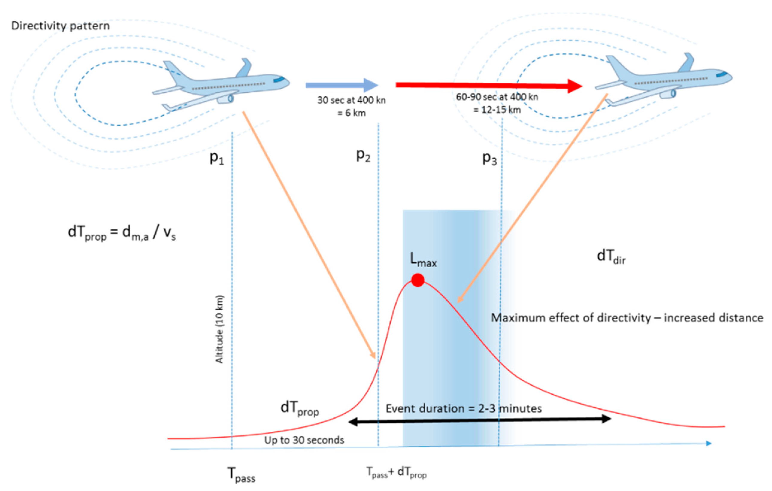
2.3. Long Distance Event Detection Is a Timely Question

The first component includes the actual event detection of aircrafts—a pass-by at a low exposure level—followed by matching the detected event to the flight responsible for the event. This exercise is less straightforward than is expected at first glance. Two physical phenomena introduce time delays between the flight passage and the detection of the maximum levels of the aircraft event: the limited speed of sound and the directivity pattern of the sound emission of the aircraft. The impact on event detection is illustrated in Figure 1. A cruising aircraft flies at a typical height of 10 km, which results in a time delay of 30 s at the typical speed of sound (340 m/s). The aircraft emission expresses a strong directivity pattern, emitting the highest sound levels at the tail [12,13,14]. The directivity pattern is sensitive to the type of aircraft and especially the engine type and engine configuration. A typical jet engine expresses the strongest emissions towards the exit of the jet engine. Strong directivity will result in even larger time delays. The maximum exposure at ground level is the combined result of the distance, altitude and directivity of the aircraft. Wind speed and wind direction will modify the maximum levels but will not impact noise event delay. In the extreme case of high-altitude cruising, an aircraft can travel up to 20 km before the peak exposure occurs.

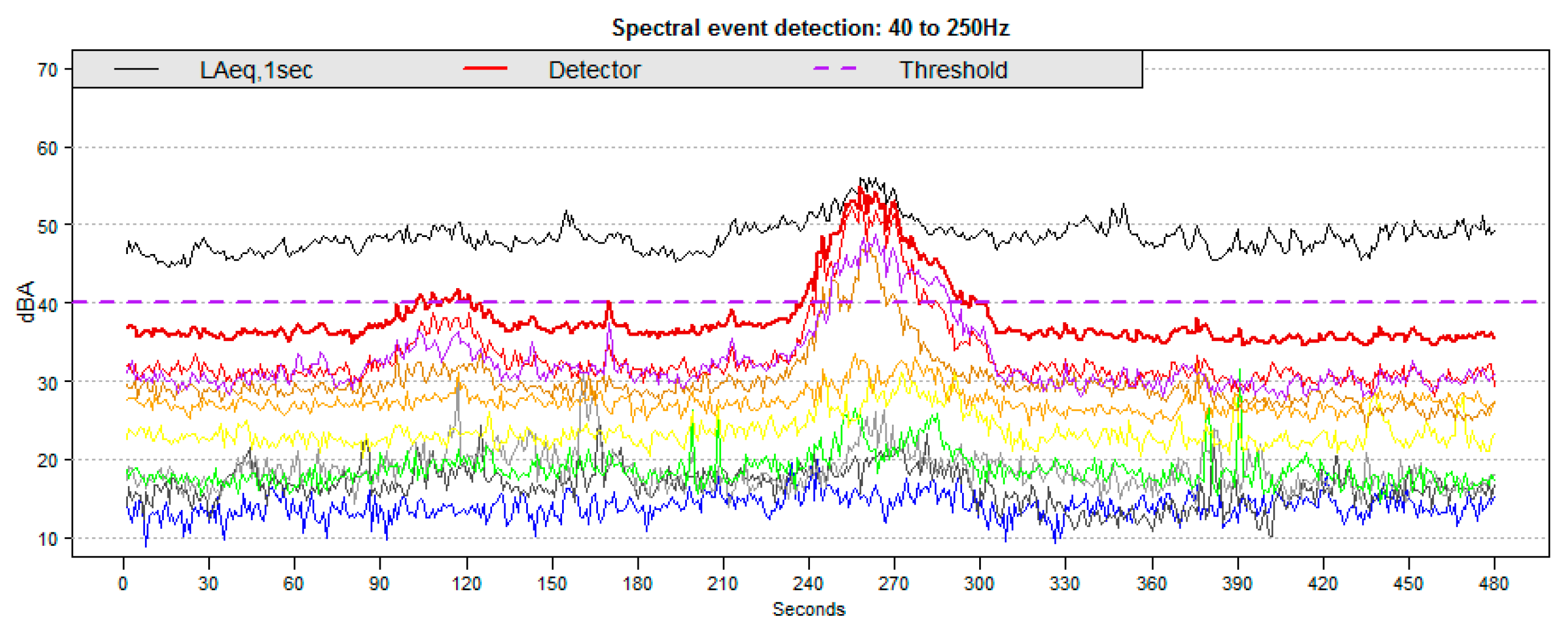
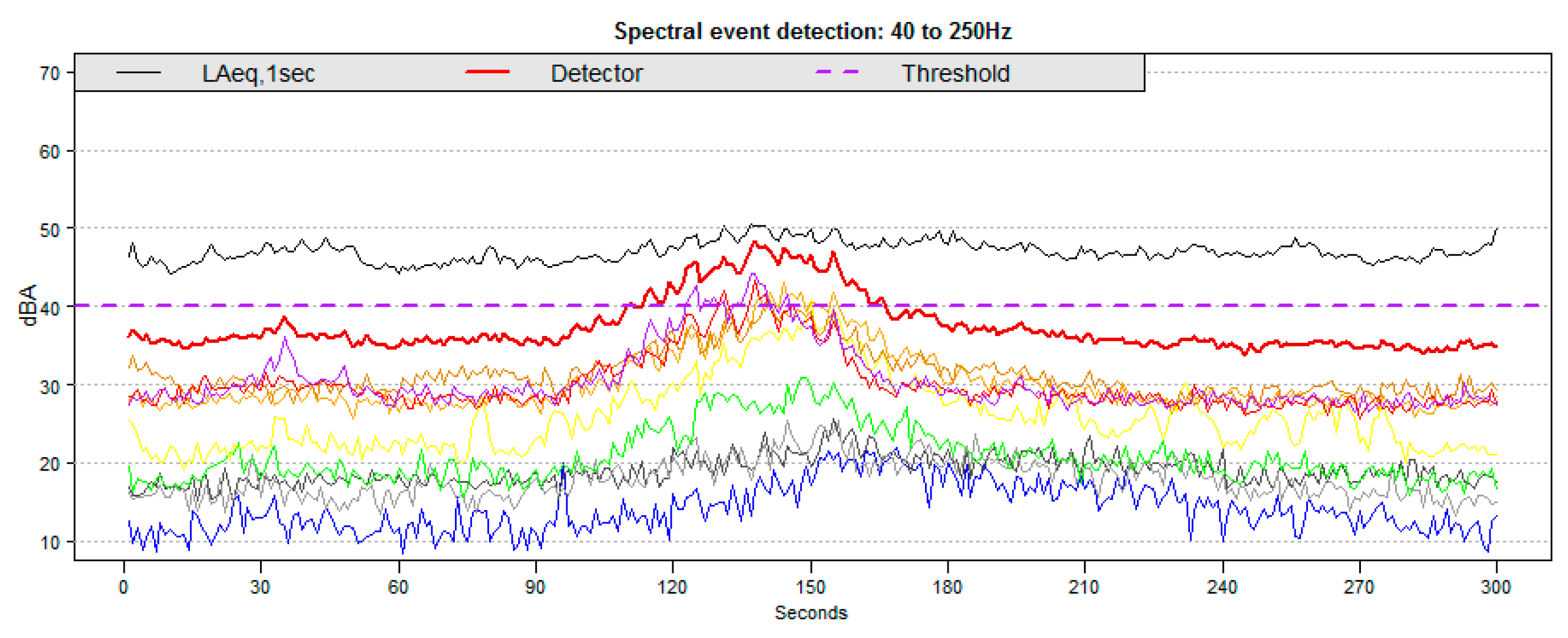
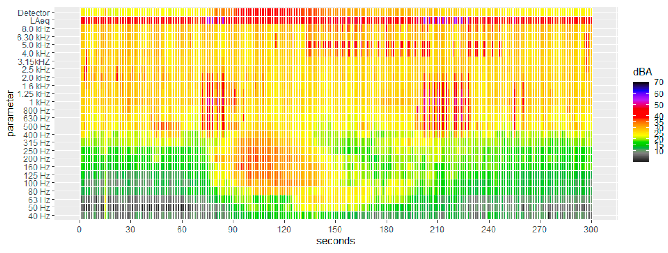
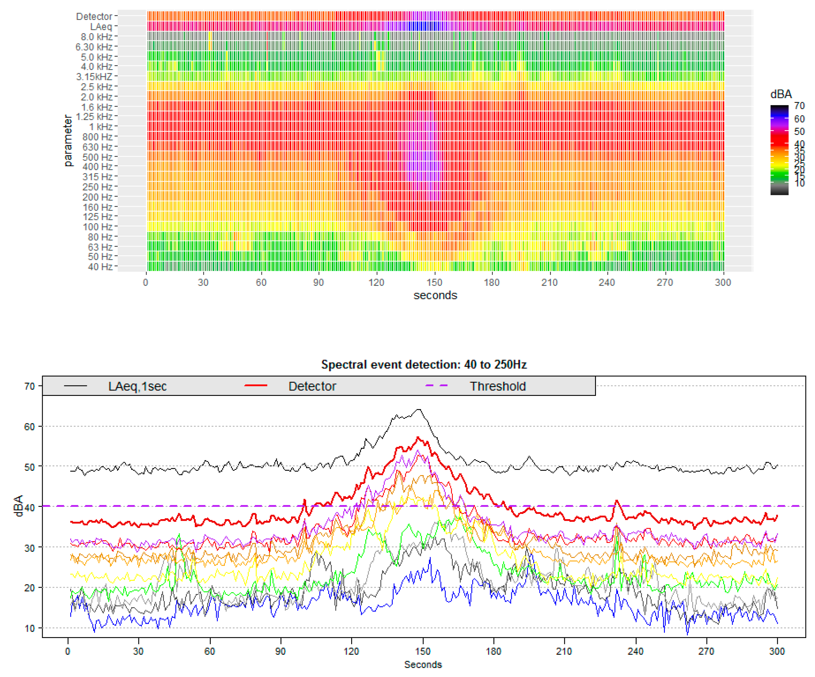
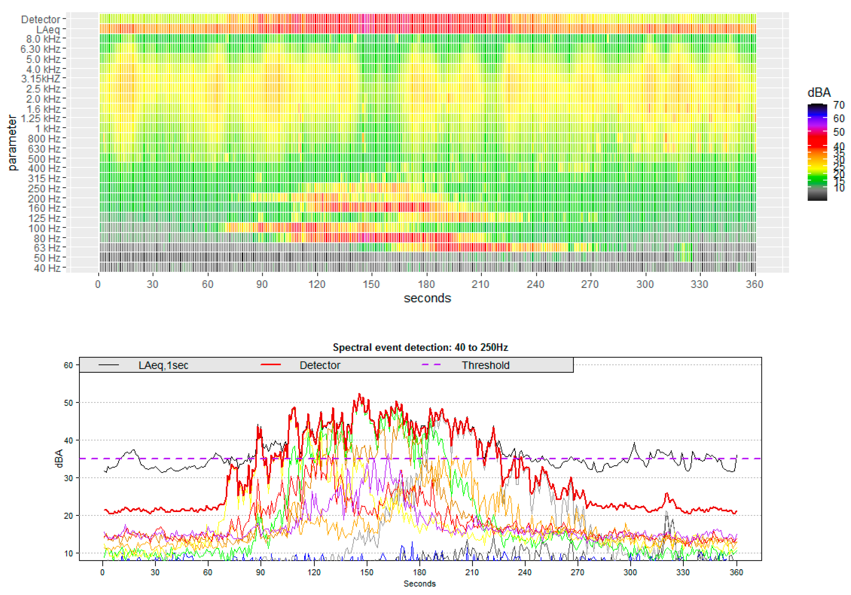
2.4. Event Detection Method

Low frequencies propagate further. At a long distance, aircraft events are detectable due to these low frequencies. An event detector is calculated by summing a set of one-third octave frequency bands (40 to 250 Hz) and detect episodes that exceed a chosen threshold TrLF for a minimum duration t. This is a very basic extension on ISO 20906:2009, but without restriction on the magnitude of the emergence of the event above ambient levels. In ISO 20906, the event duration is a function of the LAmax and is limited to the time window LAmax—10 dB. In this approach, the event duration will not be defined explicitly yet, but this attribute should emerge as a result from the exposure modeling in the second phase. Especially the long tail of low-frequency noise might extend the event duration. The definition of the event duration will depend on the state-of-the-art knowledge of sleep disturbances.

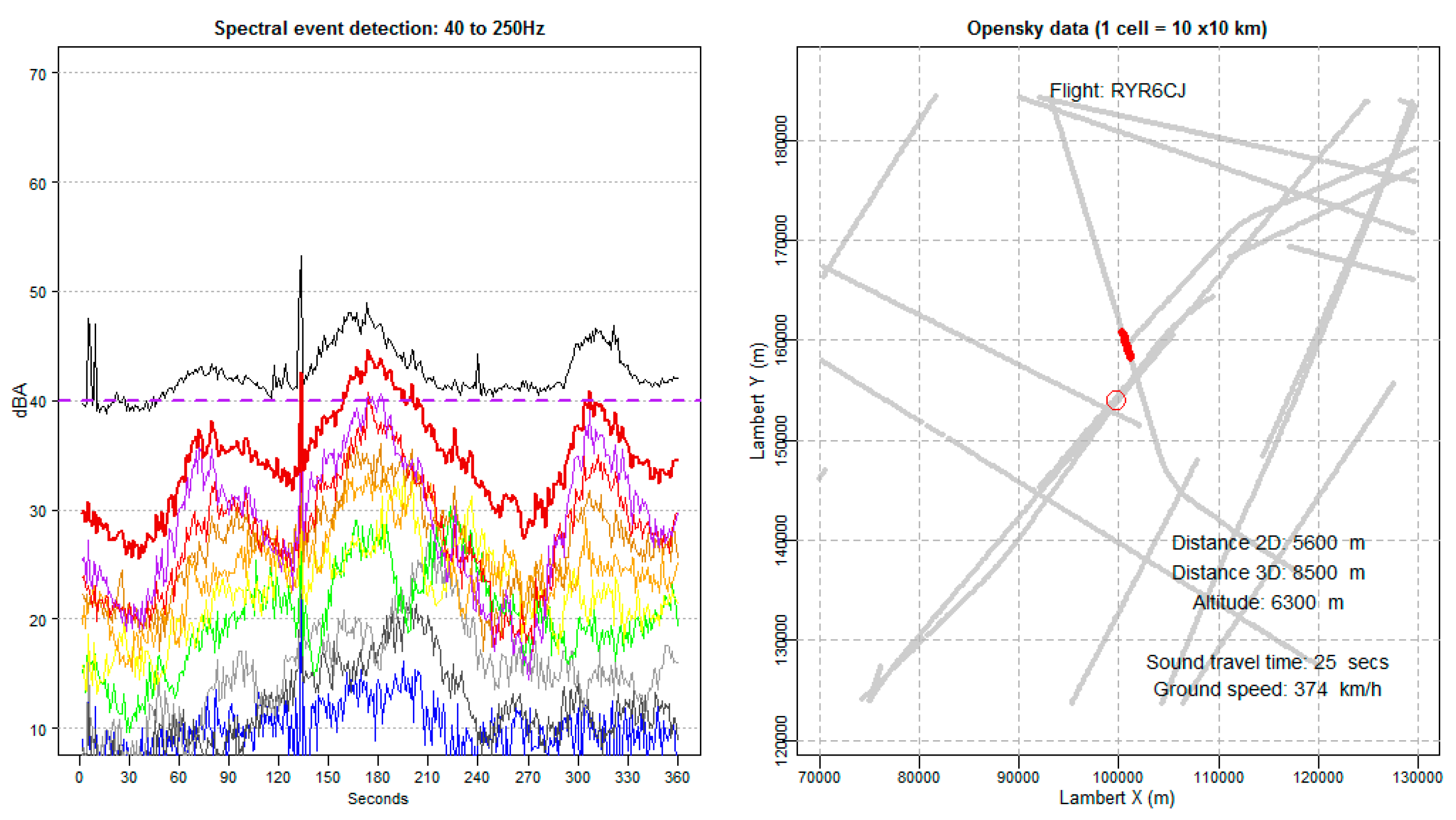
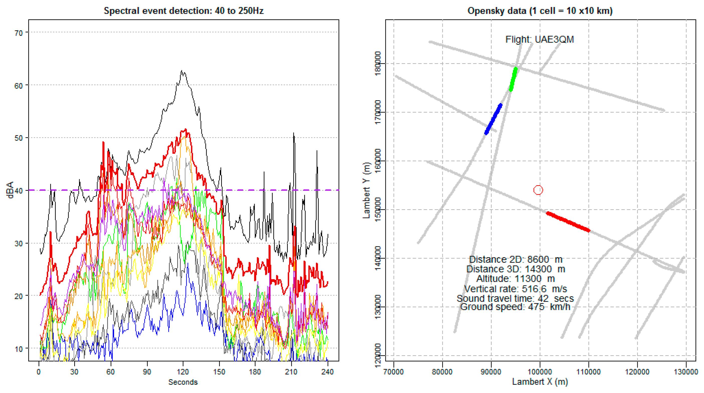
2.5. Flight Correlation Method

In this step, the impact of the speed of sound is included to match the aircraft pass-by in time and space to the detected event. Once an event is detected, the low-frequency noise event window LLF,T,w is used to retrieve the flight data near the measurement location during this event. This time window LLF,T is expanded to include at least three minutes before and after the noise event LLF,T,e. The spatial search window MPbox is set to a 30-km horizontal distance. At this point, the ADS-B records are queried for the OpenSky database, using the available Python library of Xavier Olive [15]. For each second, the following parameters are calculated: 3D distance between the aircraft D3d,sr, sound propagation time Tprop,3d and sound arrival time Tarr,3d. When the window of the sound arrival time Tarr,3d,w matches the detector window LLF,T,w, the matching flight is identified. Note that the low-frequency-based event detector is sensitive to the low-frequency tail, which is the result of the directivity pattern of the aircraft. The low-frequency detector is, by design, sensitive to the time delays related to the directivity pattern. This last phase is critical to validate the exposure model since the closest aircraft at a given time is not necessarily the noise source of the detected event. Evidently, overlaps of sound immission of multiple flights are possible. Colliding events will be excluded from the dataset used to develop the exposure model.

2.6. Modeling the Correlated Events

This part of the methodology is out of the scope of this publication, but for each event, all physical features affecting the sound propagation are estimated. Two sets can be identified: source emission-related and meteorological disturbances. The actual distance, the bearing and azimuth will be sensitive to the attenuation by distance and the directivity of the noise emission of the aircraft. The propagation of the noise towards the immission point will also be affected by wind speed and wind direction. This will result in a spatiotemporal exposure model sensitive to the distance to the source, aircraft type, including the directivity pattern, and the meteorological conditions.

3. Results

3.1. Event Detection

In the following section, a few typical examples of detected noise aircraft noise events are shown in Figure 2, Figure 3, Figure 4 and Figure 5 to illustrate the validity. The spectrograms show the time in seconds at the horizontal axis and the spectral bands on the vertical axis. The total LAeq,1sec and the detector value are included in the spectrogram. The time series show the LAeq,1sec in black at the top; the thick red line is the event detector. The purple dotted line is the applied threshold for that specific location. The other lines show the behavior of the individual spectral band in the range of 40 to 250 Hz; 40 Hz is blue, 100 Hz is yellow and two variants of orange, red and purple are the bands 125 to 250 Hz. The higher-frequency bands are not shown in the plot to avoid cluttering.
Few typical features are of interest. First, the tail of the event contains typically lower frequencies. This has two main origins: low frequencies propagate further and the frequency at the receiver is modified due to the Doppler effect. Approaching aircraft noise is detected at higher frequencies than the emitted sound, receding aircraft noise at lower frequencies. In Figure 5, the Doppler effect is illustrated with a tonal event of a propeller aircraft.

3.2. Flight Correlation

Once the flight data and the sound arrival time window are combined, the potential flights can be listed. For each of the flights, the arrival time window Tarr,3d,w is calculated. In Figure 6, an example is shown in busy skies. Three consecutive events illustrate that the method is able to identify the flight matching the detected event.
In Figure 7, an example is shown with three colliding events. The main event is linked to a flight passing from west to east to the south of the measurement point, but at the start of the event, it is disturbed by two other flights going from south to north. This event will be excluded from the modeling dataset.

4. Discussion

4.1. General

It is clear that event detection using third-octave band measurements is successful. The event can be detected in high ambient noise levels due to the distinctive spectral content of the aircraft events. Detected events can be related to the flight information available through ADS-B messages very accurately. Including physical information on the speed of sound to adjust for the sound arrival time at the receiver is relevant to distinguish between consecutive events. An additional complication is the strong directivity of the aircraft noise sources. This does not affect the detection potential and this information will add value in the noise exposure model that will be built using this data collection. Background noise levels have a distinctive diurnal pattern and will also increase at higher wind speeds. The methodology will be extended with a variable threshold setting.
False positives should be avoided since inclusion of immission data in the noise exposure model will reduce the quality of the model. Two approaches will be tested. First, additional indicators will be defined to identify the shape of the event and distinguish the aircraft events from other environmental sources. Railway events are a specific target, but since the data are also collected in industrial settings, other event-like sources have to be excluded.
The noise exposure model should be sensitive to aircraft type and operational settings (descending, ascending or cruising). If the distance between the source and the receiver is large, the impact of wind speed is to be expected. A flight passing the receiver under upwind conditions will result in lower exposure levels. The directivity of the aircraft noise source affects the temporal pattern of the noise exposure. Detecting events in various configurations will reveal the directivity patterns of specific aircrafts. This should result in a spatiotemporal function predicting the LAmax and SEL. Spectral content will be included but the final immission parameters are not defined at this stage.

4.2. Aircraft Noise Emission Classification

Selecting the most probable correlating aircraft is evidently affected by the noise aircraft type. The OpenSky database does not provide structured aircraft identification. Linking the aircraft to the proper aircraft type and to the matching noise emission category in the ANP database is crucial for the quality of the resulting noise event prediction model. Improving the quality of the aircraft table in the OpenSky setup will simplify this step in the event prediction model.

4.3. Relevancy for Aircraft Annoyance, Complaints and Health Impact

As mentioned before, annoyance is reported well outside the limits of reporting imposed by the Environmental Noise Directive (Lden 55 dBA). The examples illustrate the impact of noisy single events over a wide area. The example of the Antonov flight is an extreme case but shows that at low-ambient-noise levels, the potential to result in awakenings and arousals is significant. An interesting potential application is the investigation of noise complaints. A simulated event statistic near the dwelling of the complainer before, during and after the complaint can explain the trigger for the complaint and improve our understanding of the complex process of annoyance and sleep disturbance. Understanding the impact of individual events is a prerequisite to transform the current noise indicator into indicators sensitive to the number of events (see recommendations of the GDG mentioned in the Introduction) [8]. The next level of implementation is to provide this functionality for sleep studies, indoor–outdoor measurement campaigns and, last but not least, full epidemiological health impact studies.

Funding

This research received no external funding.

Acknowledgments

The author would like to thank the OpenSky Network for granting access to the OpenSky database for this research.

Conflicts of Interest

The author declares no conflict of interest.

References

  1. Europa, E.U. Directive 2002/49/EC of the European Parliament and of the Council of 25 June 2002 Relating to the Assessment and Management of Environmental Noise; Europa EU: Brussels, Belgium, 2002. [Google Scholar]
  2. EASA. European Aviation Environmental Report 2019; EASA: Cologne, Germany, 2019. [Google Scholar] [CrossRef]
  3. Asensio, C.; Recuero, M.; Ruiz, M. Aircraft noise-monitoring according to ISO 20906. Evaluation of uncertainty derived from the classification and identification of aircraft noise events. Appl. Acoust. 2012, 73, 209–217. [Google Scholar]
  4. Genesca, M.; Romeu, J.; Pamies, T.; Sanchez, A. Aircraft noise monitoring with linear microphone arrays. IEEE Aerosp. Electron. Syst. Mag. 2010, 25, 14–18. [Google Scholar] [CrossRef]
  5. Rosin, C.; Barbo, B. Aircraft noise monitoring: Threshold overstepping detection vs. noise level shape and audio pattern recognition detection. Internoise 2013, 2011, 15–18. [Google Scholar]
  6. The Aircraft Noise and Performance (ANP) Database: An International Data Resource for Aircraft Noise Modellers. Available online: https://www.aircraftnoisemodel.org/ (accessed on 1 October 2020).
  7. WORLD Health Organization. Burden of Disease from Environmental Noise: Quantification of Healthy Life Years Lost in Europe; World Health Organization, Regional Office for Europe: København, Denmark, 2011. [Google Scholar]
  8. World Health Organization. Environmental Noise Guidelines for the European Region; WHO: Geneva, Switzerland, 2018. [Google Scholar]
  9. Geluidshinder—Evaluatie van de MIRA Indicatorset. Available online: https://www.milieurapport.be/publicaties/2020/geluidshinder-evaluatie-van-de-mira-indicatorset (accessed on 1 October 2020). (In Dutch).
  10. Dobruszkes, F.; Efthymiou, M. When environmental indicators are not neutral: Assessing aircraft noise assessment in Europe. J. Air Trans. Manag. 2020, 88, 101861. [Google Scholar] [CrossRef]
  11. Schäfer, M.; Strohmeier, M.; Lenders, V.; Martinovic, I.; Wilhelm, M. Bringing Up OpenSky: A Large-scale ADS-B Sensor Network for Research. In Proceedings of the 13th IEEE/ACM International Symposium on Information Processing in Sensor Networks (IPSN), Berlin, Germany, 15–17 April 2014; pp. 83–94. [Google Scholar]
  12. Pietrzko, S.; Hofmann, R.F. Prediction of A-weighted aircraft noise based on measured directivity patterns. Appl. Acoust. 1988, 23, 29–44. [Google Scholar] [CrossRef]
  13. Pietrzko, S.; Bütikofer, R. FLULA-Swiss aircraft noise prediction program. In Proceedings of the Innovation in Acoustics and Vibration, Annual Conference of the Australian Acoustical Society, Adelaide, Australia, 13–15 November 2002; pp. 13–15. [Google Scholar]
  14. Zellmann, C.; Wunderli, J.M. Influence of the atmospheric stratification on the sound propagation of single flights. In Proceedings of the INTER-NOISE and NOISE-CON Congress and Conference, Melbourne, Australia, 16–19 November 2014; Volume 249, pp. 3770–3779. [Google Scholar]
  15. GitHub. Available online: https://github.com/xoolive/opensky_data (accessed on 1 October 2020).
Figure 1. The propagation time of sound affects the correlating noise event significantly for high-altitude flights. At an altitude of 12 km, the event starts about 30 s after the closest point to the receiver. The directivity of the sound emission of the aircraft results in peak immission 60–90 s later. The aircraft can travel up to 20 km before the peak exposure occurs.
Proceedings 59 00013 g001
Figure 2. Spectrogram in third-octave bands of a low-exposure aircraft event (in dBA). The aircraft event is the blob between 90 and 150 s (top). The same event as a time series with LAeq,1sec (black), the detector (red) and the detection threshold (purple dotted line) (bottom).
Proceedings 59 00013 g002aProceedings 59 00013 g002b
Figure 3. Time series of a standard event with LAmax of 65 dBA that could/should be detected with ISO 20906:2009; the detector threshold is set to 52 dBA, showing LAeq,1sec, the detector and the detection threshold (40 dBA). The third-octave bands used in the detector are also shown (40–250 Hz). Higher-frequency bands are attributed significantly to the aircraft sound exposure level (SEL).
Proceedings 59 00013 g003
Figure 4. Three time series of a events with LAmax below 50 dBA at ambient levels of 45–48 dBA.
Proceedings 59 00013 g004aProceedings 59 00013 g004b
Figure 5. Tonal spectrogram in third-octave bands of a propeller aircraft event with a duration of 3.5 min (Antonov AN-12BK Ukraine Air Alliance). The shift in spectral content from high to low is the result of the Doppler effect increasing the frequency at the receiver for an approaching source and decreasing for a receding source. The LAmax is 50 dBA for a pass-by at a 15-km horizontal distance and an altitude of 6500 m with horizontal speed of 250 km/h and a vertical speed of 0 m/s.
Proceedings 59 00013 g005
Figure 6. Noise time series with three consecutive events (left) and flight data (right) for the LLF,T,e window and the MPbox. One event triggers the selected threshold. The sound arrival time window, matching the detector window LLF,T,w, is highlighted in the flight data. A lower threshold is capable of identifying each of the three events individually.
Proceedings 59 00013 g006
Figure 7. Colliding events (left) and flight data (right) for the LLF,T,e window and the MPbox. The sound arrival time windows of three flights match the detector windows LLF,T,w and are highlighted in the flight data.
Proceedings 59 00013 g007
Publisher’s Note: MDPI stays neutral with regard to jurisdictional claims in published maps and institutional affiliations.

