Abstract
There is a growing dependence of critical and safety-of-life systems on the Global Navigation Satellite System (GNSS). GNSS interference events can cause severe impacts on aircraft safety, including unavailability of GNSS-based landing services. Therefore, it is important to be able to identify, localize, and remove interference sources that may cause these impacts. This project concentrates on events that affect the the airport environment and aims to provide improved situational awareness and safety for local airspace users. This paper contains three main sections: OpenSky ADS-B data processing, interference event characterization, and interference source localization. Specifically, we identified and removed incorrect timestamps from ADS-B ground receivers. We characterized the impact of interference events based on reported interference events that occurred at a San Francisco bay area airport. In addition, we designed a convex optimization model for localizing the interference sources given the ADS-B measurement. This article looks at common characteristics caused by the impact of interference events and shows a possible way to localize interference sources using ADS-B data.
1. Introduction
Radio Frequency Interference (RFI) sources can cause denial of GNSS-based landing services for aircraft that are on approach. This sudden loss of navigation is a safety issue as the landing phase is the most vulnerable flight segment. It is important to be able to detect and localize RFI sources rapidly, so that they may be turned off as quickly as possible. When interference does impact aircraft around an airport, we want to give air traffic controllers, pilots, and operational planners an overall picture of the impact of that interference event. This project uses ADS-B reports as an input data source. Aircraft broadcast their GNSS-derived position information through ADS-B to the ground stations. These crowdsourced data offer broader coverage of the impacted airspace. Similarly, the system can offer positive evidence when GPS is currently functioning well and provide air traffic controllers improved situational awareness.
This project was motivated by three reported GNSS interference events that impacted flights on approach to a local airport. Pilots of those three flights were unable to complete their intended GNSS approach procedure due to the GNSS interference. Those three flights experienced interference effect at a very similar location. One of the pilots recorded video of the GNSS receiver display during the event. These externally identified interference events provide us with a unique opportunity to characterize the impact of RFI on ADS-B output. This project uses ADS-B data from the OpenSky Network which is a community-based receiver network that collects ADS-B data and stores historical data [1]. Our goal is to analyze the capabilities and limitations of crowdsourced ADS-B data for RFI detection and localization. In addition, we also want to develop a strategy to localize interference sources using the characterized effects.
Several groups have also been working on GNSS interference detection and localization using ADS-B data. Researchers from EUROCONTROL have looked at ways of interference source localization using ADS-B [2]. They designed a grid probability model to generate heat maps for GNSS affected regions in the eastern Mediterranean. Those heat maps show possible locations of the RFI sources. Other researchers from New York University have proposed using distribution curve of NACp to identify the presence of GNSS jamming events for a given airspace [3].
This article looks at key steps to process OpenSky ADS-B raw position messages. This article concentrates on characterizing the impact of GNSS interference events happening near to airports. This article examines a way of using convex optimization for interference source localization. The overall goal is to form a strategy of processing given ADS-B raw messages, identify the presence of interference event, and localize the interference source which can then be turned off. This overall strategy provides for both improved situational awareness and increased safety.
2. Materials and Methods
2.1. OpenSky ADS-B Data Processing
This project processes ADS-B data following the procedure shown in Figure 1. An ADS-B receiver transmits a 112 bits long raw position message every 0.5 s. These raw position messages are recorded by the OpenSky network and decoded following the documentation in ADS-B-In Application MOPS [4]. The decoded message contains information about GNSS-based aircraft position and its corresponding integrity bound. However, the message does not contain time information. To have a correct time sequence, we rely on timestamps that are recorded by ADS-B ground receivers. Rather than using GNSS UTC measure time data, ADS-B ground receivers establish their own internal clocks or counters. Even though their clock time could be synchronized by the Linux NTP services, there are still some receivers showing non-standard behavior such as having inconsistent timestamps. Since having incorrect timestamp is equivalent of having wrong position information, those non-standard ADS-B receivers need to be filtered out. In the end, we obtain a csv file which contains information including time, latitude (lat), longitude (lon), and altitude (alt).
Figure 1.
Flowchart of ADS-B data processing.
2.2. Interference Events Characterization
This paper examines an area around Hayward Executive Airport (KHWD) in Hayward, CA and is based on pilot and FAA reports of suspected GNSS interference from early 2019. The reports identified a common region where flights were impacted. Therefore, we selected an airspace which covers the area where the interference event was documented. Figure 2 shows a top down view of the ADS-B data queried from the OpenSky network. Each green line represents a flight path of an aircraft entering and leaving our target airspace. The black line is the boundary of our target airspace. HWD airport is on the left upper corner of the target airspace.
Figure 2.
Top view of ADS-B data at KHWD airport.
This paper analyzes flights from January 2019 to March 2019, as well as flights from January 2020 to April 2020. Table 1 shows information on the days and flights analyzed. During those six months, we found only 22 days that appeared to contain interference events; thus, the interference events at HWD are intermittent and we were unable to identify a pattern.
Table 1.
Numbers of days and flights.
2.3. Interference Sources Localization
Once we understand the impacts and characters of interference events, we could then use some of the observed properties to detect and localize the interference source. In this project, we apply convex optimization to design one possible way for localization. At the current stage, this mathematical model is designed for simplified cases which satisfied following assumptions.
2.3.1. Assumptions
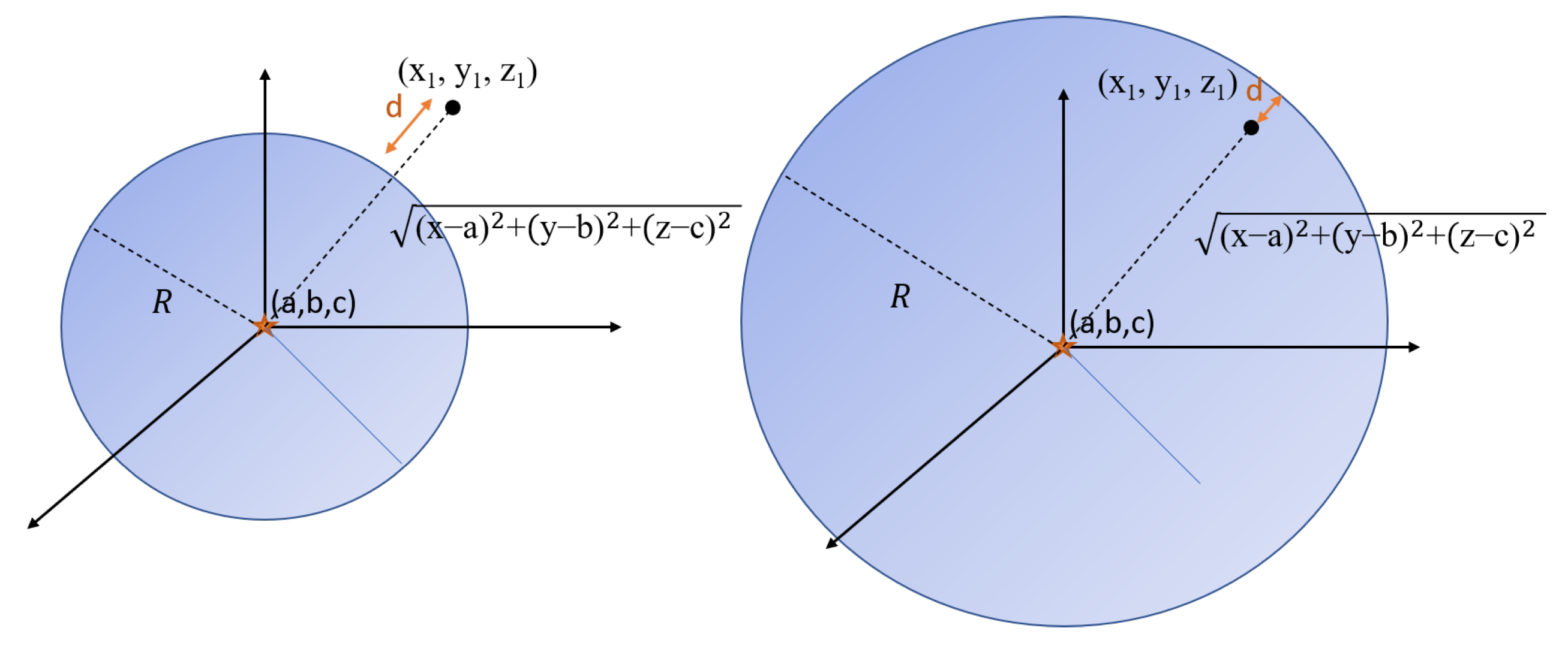
- This paper assumes the interference source radiates equally strong signal in all directions. The affected area of the interference source is modeled as a sphere.
- The RFI source is continuously emitting jamming signal and has a constant power over time. Therefore, the gaps in flight trajectory are direct results from aircraft entering the affected area. In addition, all aircraft at the same location should be affected by same power strength.
- The airspace has sufficient coverage by ADS-B ground receivers and the jamming signal of interference source is not blocked by mountains or buildings.
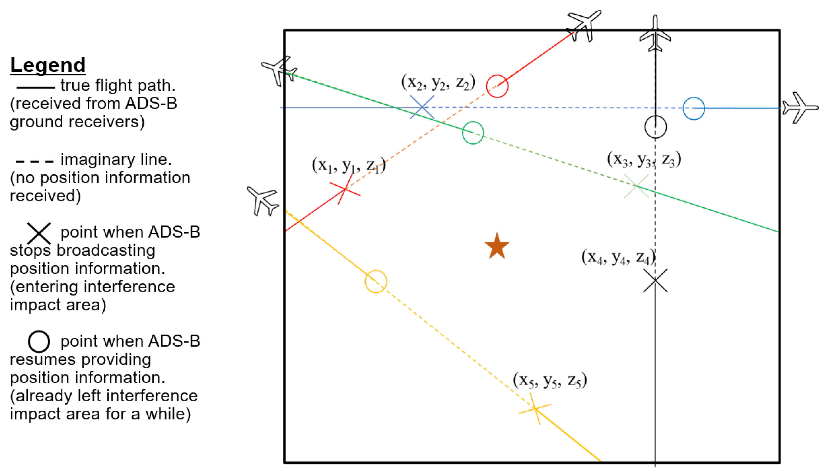
2.3.2. Impact of Interference Events
Figure 3 shows a top view of a hypothetical airspace under impact of interference event. This diagram represents what we may commonly observe during interference events. Imagine there is an interference source located at the orange star, if it is powerful enough, all aircraft entering and leaving the affected area of that RFI source would have gaps in their full flight paths. The cross marker shows the starting point of the gap in each ADS-B flight trajectory. The circle marker shows the ending point of each gap. Based on our assumption, we could say that the starting point of the gap is the exact point when aircraft starts entering the GNSS affected regions. However, the ending point of the gap is less predictable and likely be further away from the boundary. This is because after leaving the affected area, the receiver may need time to perform acquisition and signal validation before they can start recalculating and broadcasting their current position information.
Figure 3.
Top view of an airspace under impact of interference event.
2.3.3. Calculation
This project takes those starting points of the gaps as an input dataset and minimizes a convex cost function in order to localize the interference sources. Figure 4 shows a 3D model of how RFI sources impact signals in its nearby airspace. (a, b, c) is the unknown location of the interference source which corresponds to (longitude, latitude, altitude). R is the unknown radius of the spherical affected area. In theory, all starting points of the gaps should be on the outer boundary of the sphere. However, the actual data will not precisely match our simplified model, therefore we can only minimize the distance from the boundary of the sphere to all starting points. We denote them as “d” in Figure 4. Therefore, our objective function is to minimize the summation of all “d”, which again are distances from input points to the boundary of the sphere.
Figure 4.
3D model of objective function.
Equation (1) is the objective function based on above physically meanings. k is the number of input data points; recall that this project takes those starting points of the gaps as input data points.
Notice that the absolute value of a convex function and the square of a convex function are not convex functions. To make our objective function convex, we first use a variable with a constraint of to replace . is an affine function which is also a convex function. In addition, since latitude and longitude are in degrees but altitude is in meters, we need to convert degree differences into distances. Therefore, the objective function becomes as what is shown in Equation (2).
Then, instead of minimizing the absolute value of , we use the objective function shown in Equation (3). is a weight parameter which controls how much the cost function penalizes over-sizing the radius. This max function always returns the maximum value between fn and . This means if is positive, the cost function will penalize both “d(i)” and “R” depending on which one is larger. happens only when the starting point of the gap is outside the boundary of the sphere, as shown on the left hand side of Figure 4. Therefore, during the beginning of that phase, this objective function will try to speed up the process of expanding the bubble, since and it wants to minimize d(i). Later, it will try to slow down the expansion process, when R becomes larger than . happens when the starting point of the gap is within the boundary of the sphere, shown on the right-hand side of Figure 4. During that phase, since is negative, the cost function will only penalize . That helps prevent the boundary of sphere from expanding too far away from input data points.
3. Results
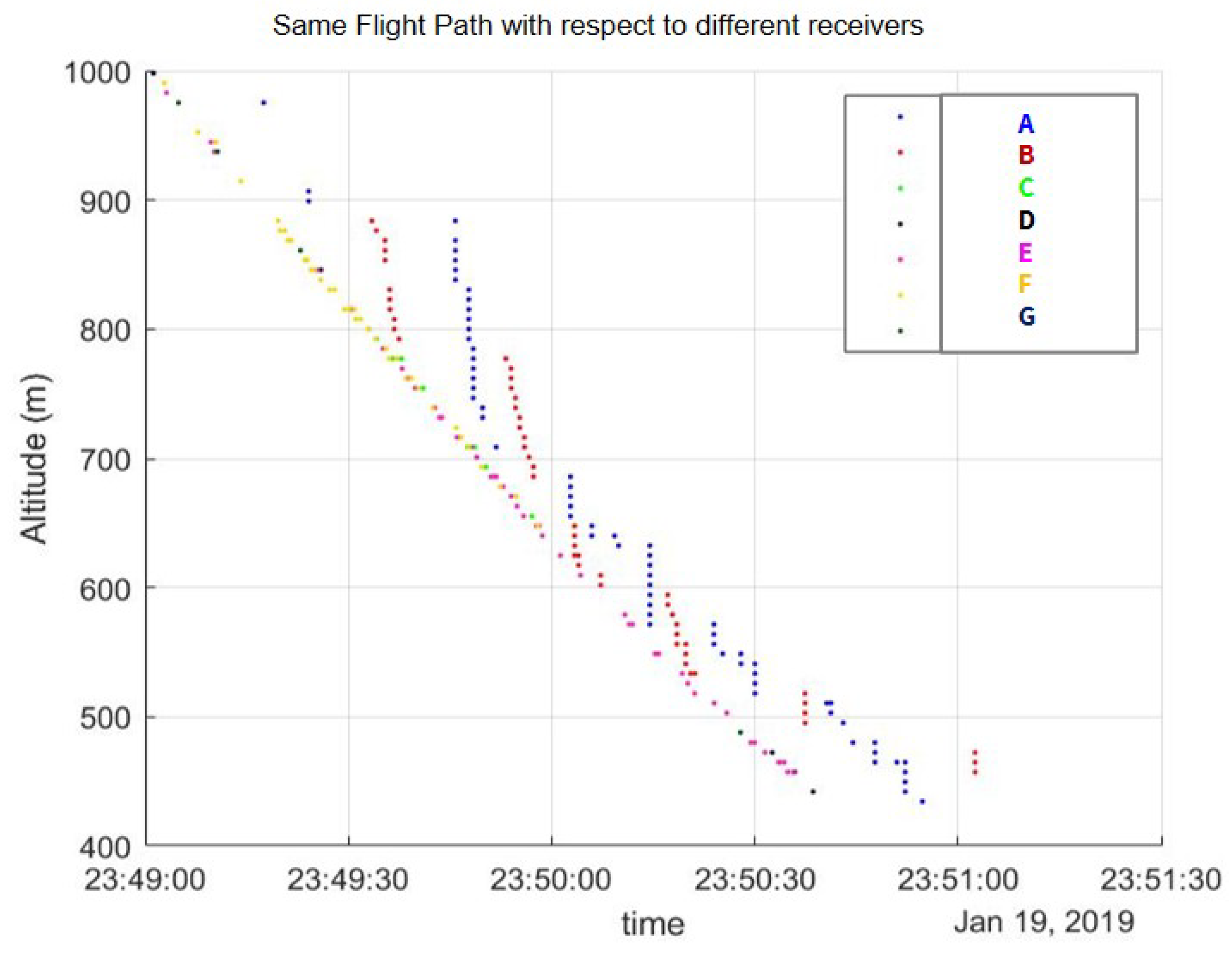
3.1. OpenSky ADS-B Data Processing
In this section, we illustrate common erroneous results caused by non-standard behavior of receiver’s internal clock. We need to detect and remove these non-standard ADS-B receivers. Further information on the causes of those incorrect timestamps could be used to improve our processing and ideally eliminate such behavior.
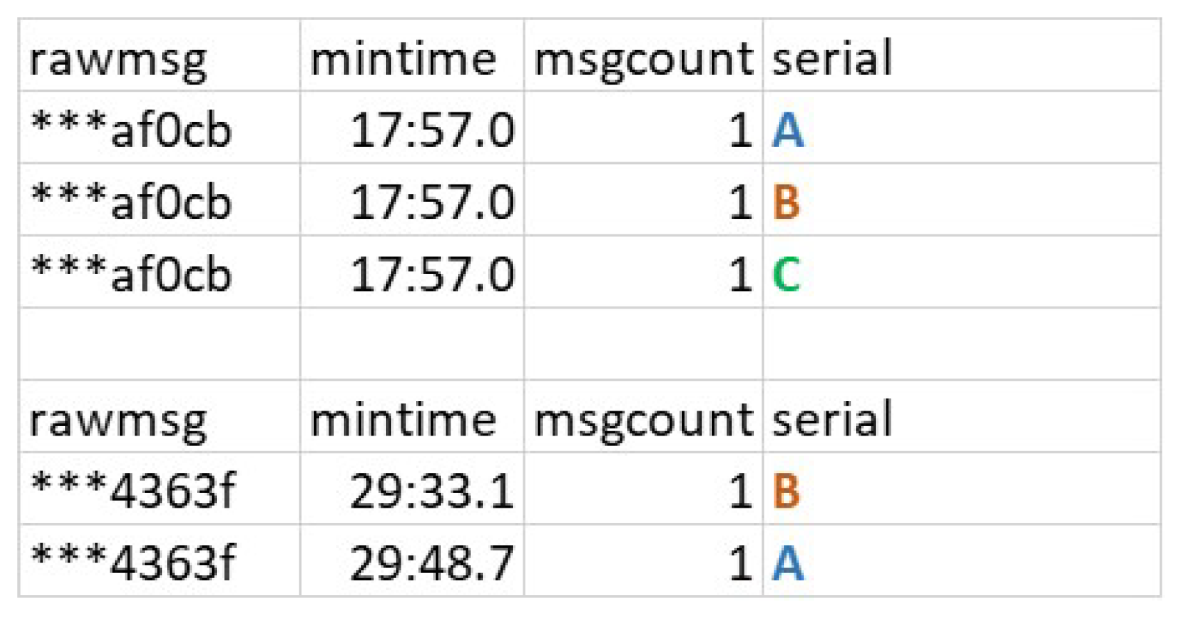
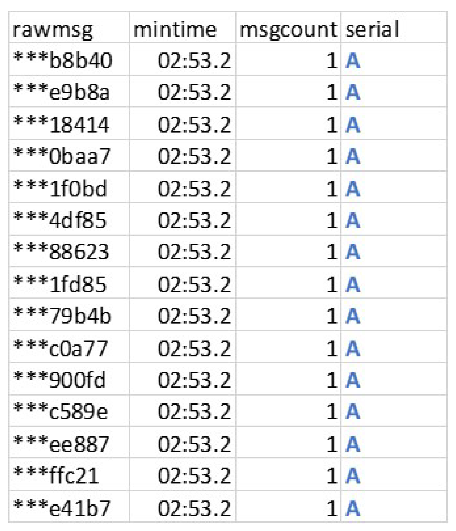
3.1.1. Inconsistent Internal Clock
The first type of non-standard ADS-B ground receiver data is the type with inconsistent time. Figure 5 shows two sets of data recorded by Receivers A–C. We used letters to replace the true serial numbers of those receivers. From left to right, Column 1 is showing the content of the raw message and part of the message information is omitted. Column 2 displays the time when the respective message was received for the first time, Column 3 indicates the number of messages that have been received at that time, and Column 4 shows the name of that receiver. Receiver A has non-standard receiver behavior. Notice that, in this sample data, the first raw message was received by all three receivers at the same time. However, the second raw message was received by Receivers A and B at different times. Figure 6 shows how that the non-standard receiver timing causes problems. It is a time versus altitude plot for same flight with respect to different ADS-B ground receivers. Blue dots represents position information received by Receiver A. Because of the inconsistent internal clock of Receiver A, the blue dotted line is slightly off-track compared with the other receivers.
Figure 5.
Sample data of receiver with inconsistent internal clock.
Figure 6.
Time versus altitude plot for same flight with respect to different receivers.
3.1.2. Incorrect Timestamp
Another type of non-standard ADS-B ground receiver behavior shows the incorrect timestamps directly. Figure 7 shows a set of sample data from Receiver A. This non-standard receiver put the same timestamp onto 15 different raw messages from the same flight. Similar behavior has also been observed for Receiver B. Noticed that, in Figure 8, Receivers A and B are showing flight paths that are not in agreement with the other receivers and that do not follow the expected approach path.
Figure 7.
Sample data of receiver with incorrect timestamp.
Figure 8.
Time versus altitude plot of same flight with respect to different receivers.
3.2. Interference Events Characterization
Figure 9 is an altitude versus time plot for all flights entering and leaving target airspace on 6 January 2019. All flight paths were plotted with dots and each dot represent one ADS-B airborne position message receiver by ground receivers. The color of each dot represents corresponding NIC value.
Figure 9.
Altitude versus time plot for all flights passing target airspace on 6 January 2019.
Most of the flights on that day behave normally with continuous reporting of position information and constant NIC value. Only two tracks have non-standard behavior and those two flights are highlighted by thicker points. The flight on the right hand side is one of the three reported RFI affected flights. It contains a position output gap that lasts for at least 10 s, and it has a change in NIC value from reasonable values above 6 down to 0 surrounding the gap. The flight on the left hand side shows a sudden drop of NIC value from 9 to 0, which was also treated as a non-standard case and likely indicates the effects of RFI. Further investigation on what causes non-standard cases is needed in the future work. By generating plots for all flights during those six months, we observed a common trend. Flights that are or might be impacted by the interference events always have a loss of airborne position and/or a drop of NIC value.
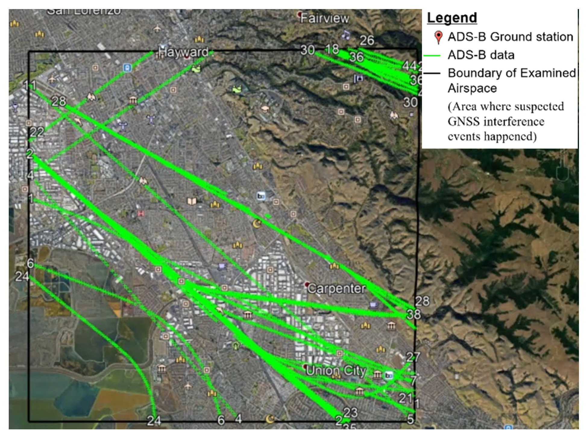
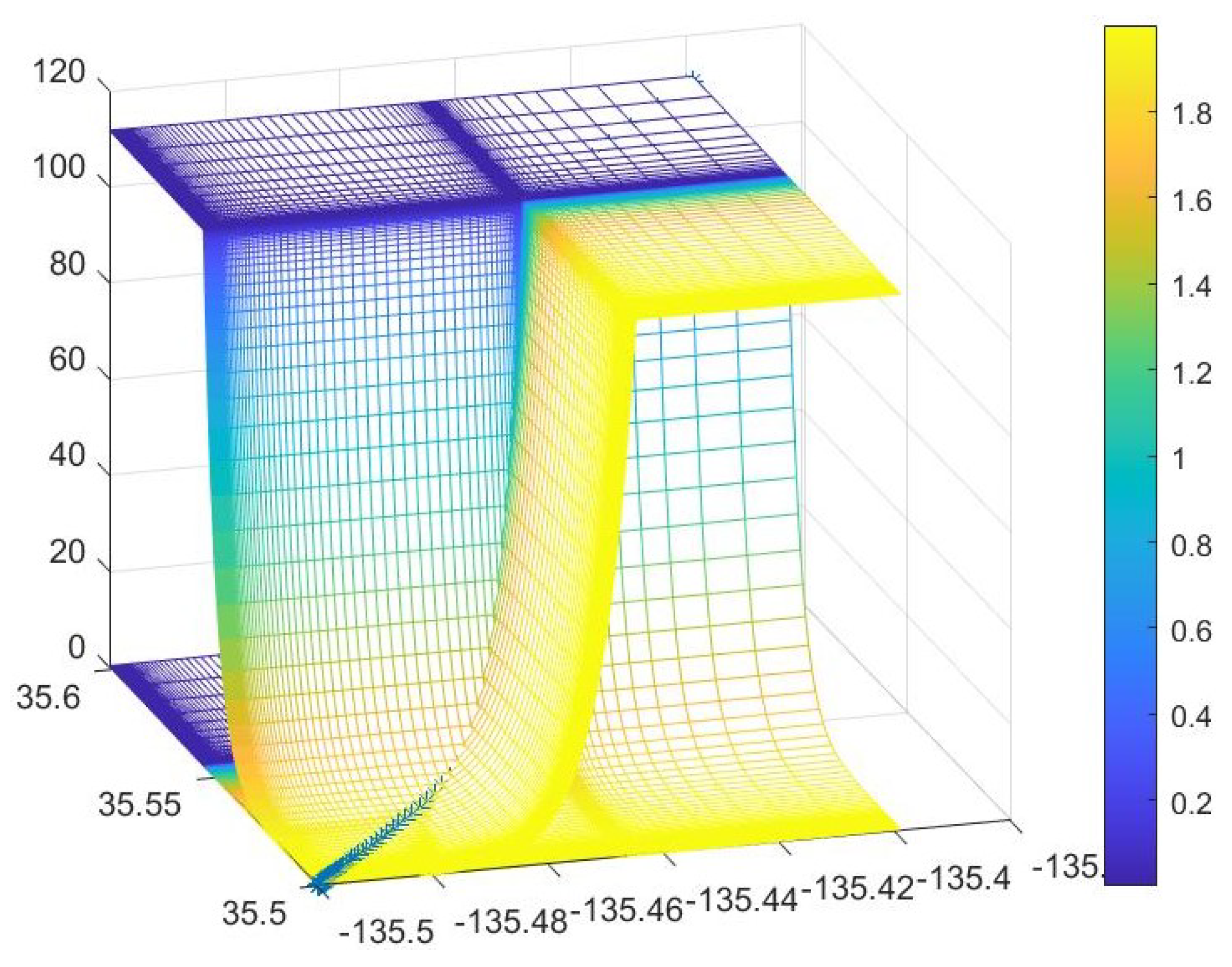
3.3. Interference Sources Localization
3.3.1. Theoretical Test
We initially tested our model with simulated data. We inputed seven points which are placed on a sphere with radius of 2. Figure 10 shows the result we obtained from our model. The red cross is the maximum likelihood location of the interference source. The sphere represents the possible size of the affected area. The calculated location of the interference source matches exactly with what it supposed to be. The calculated radius value is 1.9781, which is close to 2.
Figure 10.
Result under theoretical test.
Figure 11 shows the heat map of the cost function (Equation (1)). The vertical axis represents value of cost function, while x and y axes are latitude and longitude. The color of the grid indicates the size of R. This heat map shows how the cost function varies with different values of x, y, and R. By converting cost function from Equation (1) to Equations (2) and (3), the results of the cost function are then constrained to always stay at the concave curve section of the heat map. This proves the convexity of our designed model since we are minimizing the cost function.
Figure 11.
Heat map of cost function.
3.3.2. Real Data Case
We then put the jammed flight data from HWD airport from the entire month of January 2019 into our model. Figure 12 shows the corresponding result. The left hand side of Figure 12 shows the results on 3D plot. Rather than being well distributed on the map, all of the starting points of the gaps are essentially on a straight line. Therefore, our fitting model can only identify the estimated RFI location along this same line. The right hand side of Figure 12 shows the results on a Google Earth map. The cyan circle is marking an industrial area that was speculated to be the source of interference. The maximum likelihood location of the interference source is marked with the red cross. Notice that the red cross is on the top corner of that industrial area. More data points ideally located away from the line would be needed to better refine the location estimate.
Figure 12.
Result from real data: on 3D plot (left); and on Google Earth map (right).
4. Discussion and Conclusions
We demonstrated that using ADS-B to provide situation awareness of the GNSS interference events is possible. Starting from reported interference events, this paper shows how we characterized the effects of interference events and used corresponding results to detect flights that are potentially jammed. In addition, this project shows a possible method to localize interference sources using convex optimization. Subsequent work will therefore investigate non-standard flight dynamic cases that may be indicative of potentially jammed flights. We further plan to improve the objective function and interference source model for localization, as well as investigate similar interference events reported at other airports. Our overall goal is to develop a method to provide airspace users improved situational awareness and safety.
Author Contributions
Z.L. developed the localization algorithm and carried out the data analysis. S.L. and T.W. directed and supervised the research work at all stages. All authors have read and agreed to the published version of the manuscript.
Funding
This work was supported by the Federal Aviation Administration Navigation Program Office under grant number 693KA8-19-N-00015.
Acknowledgments
The authors thank the OpenSky network for providing data for this study.
Abbreviations
The following abbreviations are used in this manuscript:
| GNSS | Global Navigation Satellite System |
| ADS-B | Automatic Dependent Surveillance-Broadcast |
| RFI | Radio-frequency interference |
| NACp | Navigation Accuracy Category—Position |
| MOPS | Minimum Operational Performance Standards |
| NTP | Network Time Protocol |
References
- Schäfer, M.; Strohmeier, M.; Lenders, V.; Martinovic, I.; Wilhelm, M. Bringing up OpenSky: A large-scale ADS-B sensor network for research. In Proceedings of the 13th International Symposium on Information Processing in Sensor Networks, Berlin, Germany, 15–17 April 2014. [Google Scholar]
- Jonáš, P.; Vitan, V. Detection and Localization of GNSS Radio Interference using ADS-B Data. In Proceedings of the 2019 International Conference on Military Technologies (ICMT), Brno, Czech Republic, 30–31 May 2019; pp. 1–5. [Google Scholar] [CrossRef]
- Darabseh, A.; Bitsikas, E.; Tedongmo, B. Detecting GNSS Jamming Incidents in OpenSky Data. EPiC Ser. Comput. 2019, 67, 97–108. [Google Scholar]
- DO-260B RTCA (Firm). Minimum Operational Performance Standards (MOPS) for 1090 MHz Extended Squitter Automatic Dependent Surveillance-Broadcast (ADS-B) and Traffic Information Services-Broadcast (TIS-B); RTCA, Incorporated: Washington, DC, USA, 2011. [Google Scholar]
Publisher’s Note: MDPI stays neutral with regard to jurisdictional claims in published maps and institutional affiliations. |
© 2020 by the authors. Licensee MDPI, Basel, Switzerland. This article is an open access article distributed under the terms and conditions of the Creative Commons Attribution (CC BY) license (https://creativecommons.org/licenses/by/4.0/).


